This paper was converted on www.awesomepapers.org from LaTeX by an anonymous user.
Want to know more? Visit the Converter page.

Compound Poisson particle approximation for McKean-Vlasov SDEs

Xicheng Zhang Xicheng Zhang: School of Mathematics and Statistics, Beijing Institute of Technology, Beijing 100081, China
Email: XichengZhang@gmail.com
Abstract.

We present a comprehensive discretization scheme for linear and nonlinear stochastic differential equations (SDEs) driven by either Brownian motions or α\alpha-stable processes. Our approach utilizes compound Poisson particle approximations, allowing for simultaneous discretization of both the time and space variables in McKean-Vlasov SDEs. Notably, the approximation processes can be represented as a Markov chain with values on a lattice. Importantly, we demonstrate the propagation of chaos under relatively mild assumptions on the coefficients, including those with polynomial growth. This result establishes the convergence of the particle approximations towards the true solutions of the McKean-Vlasov SDEs. By only imposing moment conditions on the intensity measure of compound Poisson processes, our approximation exhibits universality. In the case of ordinary differential equations (ODEs), we investigate scenarios where the drift term satisfies the one-sided Lipschitz assumption. We prove the optimal convergence rate for Filippov solutions in this setting. Additionally, we establish a functional central limit theorem (CLT) for the approximation of ODEs and show the convergence of invariant measures for linear SDEs. As a practical application, we construct a compound Poisson approximation for 2D-Navier Stokes equations on the torus and demonstrate the optimal convergence rate.


Keywords: Compound Poisson approximation, McKean-Vlasov stochastic differential equation, Invariance measure, Navier-Stokes equation, Central Limit Theorem.

AMS 2010 Mathematics Subject Classification: 65C35, 60H10, 35Q30

This work is partially supported by NNSFC grants of China (Nos. 12131019), and the German Research Foundation (DFG) through the Collaborative Research Centre(CRC) 1283 “Taming uncertainty and profiting from randomness and low regularity in analysis, stochastics and their applications”.

1. Introduction

Let σ:+×d×ddd\sigma:{\mathbb{R}}_{+}\times{\mathbb{R}}^{d}\times{\mathbb{R}}^{d}\to{\mathbb{R}}^{d}\otimes{\mathbb{R}}^{d} and b:+×d×ddb:{\mathbb{R}}_{+}\times{\mathbb{R}}^{d}\times{\mathbb{R}}^{d}\to{\mathbb{R}}^{d} be two Borel measurable functions. Throughout this paper, for a probability measure μ\mu over d{\mathbb{R}}^{d}, we write

σ[t,x,μ]:=dσ(t,x,y)μ(dy),b[t,x,μ]:=db(t,x,y)μ(dy).\sigma[t,x,\mu]:=\int_{{\mathbb{R}}^{d}}\sigma(t,x,y)\mu({\mathord{{\rm d}}}y),\ \ b[t,x,\mu]:=\int_{{\mathbb{R}}^{d}}b(t,x,y)\mu({\mathord{{\rm d}}}y).

Fix α(0,2]\alpha\in(0,2] and consider the following McKean-Vlasov SDE or distribution-dependent SDE (abbreviated as DDSDE):

dXt=σ[t,Xt,μt]dLt(α)+b[t,Xt,μt]dt,\displaystyle{\mathord{{\rm d}}}X_{t}=\sigma[t,X_{t},\mu_{t}]{\mathord{{\rm d}}}L^{(\alpha)}_{t}+b[t,X_{t},\mu_{t}]{\mathord{{\rm d}}}t, (1.1)

where μt=μXt\mu_{t}=\mu_{X_{t}} denotes the probability distribution of XtX_{t}, Lt(2)=WtL^{(2)}_{t}=W_{t} stands for a dd-dimensional standard Brownian motion, and for α(0,2)\alpha\in(0,2), Lt(α)L^{(\alpha)}_{t} is a symmetric and rotationally invariant α\alpha-stable process with infinitesimal generator Δα/2\Delta^{\alpha/2} (the usual fractional Laplacian operator).

In the literature, DDSDE (1.1) is also considered as a nonlinear SDE due to the dependence of its coefficients on the distribution of the solution. By applying Itô’s formula, μt\mu_{t} solves the following nonlinear Fokker-Planck equation in the distributional sense:

tμt=t,μtμt,\partial_{t}\mu_{t}={\mathscr{L}}^{*}_{t,\mu_{t}}\mu_{t},

where t,μ{\mathscr{L}}^{*}_{t,\mu} is the adjoint operator of the generator (local/nonlocal ) of SDE (1.1): for α=2\alpha=2,

t,μf(x):=12tr(σ[t,x,μ]σ[t,x,μ]2f(x))+b[t,x,μ]f(x),{\mathscr{L}}_{t,\mu}f(x):=\tfrac{1}{2}\mathrm{tr}{\big{(}}\sigma[t,x,\mu]\sigma^{*}[t,x,\mu]\cdot\nabla^{2}f(x){\big{)}}+b[t,x,\mu]\cdot\nabla f(x),

and for α(0,2)\alpha\in(0,2),

t,μf(x):=p.v.df(x+σ[t,x,μ]z)f(x)|z|d+αdz+b[t,x,μ]f(x),{\mathscr{L}}_{t,\mu}f(x):={\rm p.v.}\int_{{\mathbb{R}}^{d}}\frac{f(x+\sigma[t,x,\mu]z)-f(x)}{|z|^{d+\alpha}}{\mathord{{\rm d}}}z+b[t,x,\mu]\cdot\nabla f(x),

where σ\sigma^{*} stands for the transpose of matrix σ\sigma and p.v. stands for the Cauchy principle value.

In the seminal work by McKean [31], the study of nonlinear SDE (1.1) driven by Brownian motions was initiated. His paper established a natural connection between nonlinear Markov processes and nonlinear parabolic equations. Since then, the McKean-Vlasov SDE has evolved into a fundamental mathematical framework, offering a powerful tool for analyzing complex systems comprising a large number of interacting particles. The McKean-Vlasov SDE discribes the dynamics of a single particle, influenced by the collective behavior of the entire system. Its applications have expanded across various fields, including statistical physics, stochastic analysis, economics, and biology. Through the study of the McKean-Vlasov SDE, researchers have gained significant understanding of diverse phenomena, ranging from the behavior of particles in statistical mechanics to intricate dynamics in economic and biological systems. Its utility extends beyond theoretical investigations, playing a vital role in the development of numerical methods, data analysis techniques, and decision-making models. For a more comprehensive overview and references, the survey paper by [6] provides valuable insights into the McKean-Vlasov SDE and its wide-ranging applications.

When bb and σ\sigma satisfy the following Lipschitz assumption

σ(t,x,y)σ(t,x,y)+|b(t,x,y)b(t,x,y)|κ(|xx|+|yy|),\displaystyle\|\sigma(t,x,y)-\sigma(t,x^{\prime},y^{\prime})\|+|b(t,x,y)-b(t,x^{\prime},y^{\prime})|\leqslant\kappa(|x-x^{\prime}|+|y-y^{\prime}|), (1.2)

it is well-known that for any initial value X0X_{0}, there is a unique strong solution to DDSDE (1.1) (see [40], [6]). From the perspective of Monte-Carlo simulations and practical applications, the McKean-Vlasov SDEs (1.1) are often approximated using an interaction particle system. In the case of Brownian motions (α=2\alpha=2), the approximation takes the following form: For fixed NN\in{\mathbb{N}}, let 𝐗N:=(XN,1,,XN,N){\mathbf{X}}^{N}:=(X^{N,1},\cdots,X^{N,N}) solve the following SDE in Nd{\mathbb{R}}^{Nd}:

dXtN,i=σ[t,XtN,i,μ𝐗tN]dWti+b[t,XtN,i,μ𝐗tN]dt,\displaystyle{\mathord{{\rm d}}}X^{N,i}_{t}=\sigma[t,X^{N,i}_{t},\mu_{{\mathbf{X}}^{N}_{t}}]{\mathord{{\rm d}}}W^{i}_{t}+b[t,X^{N,i}_{t},\mu_{{\mathbf{X}}^{N}_{t}}]{\mathord{{\rm d}}}t, (1.3)

where {Wi,i=1,2,}\{W^{i},i=1,2,\cdots\} is a sequence of i.i.d. Brownian motions, and for a point 𝐱=(x1,,xN)(d)N{\mathbf{x}}=(x^{1},\cdots,x^{N})\in({\mathbb{R}}^{d})^{N}, the empirical measure of 𝐱{\mathbf{x}} is defined by

μ𝐱(dz):=1Ni=1Nδxi(dz)𝒫(d),\mu_{{\mathbf{x}}}({\mathord{{\rm d}}}z):=\frac{1}{N}\sum_{i=1}^{N}\delta_{x^{i}}({\mathord{{\rm d}}}z)\in{\mathcal{P}}({\mathbb{R}}^{d}),

where δxi\delta_{x^{i}} is the usual Dirac measure concentrated at point xix^{i}. Under Lipschitz assumption (1.2), it is well-known that for any T>0T>0, there is a constant C>0C>0 such that for any NN\in{\mathbb{N}},

supi=1,,N𝔼(supt[0,T]|XtN,iX¯ti|2)CN,\sup_{i=1,\cdots,N}{\mathbb{E}}\left(\sup_{t\in[0,T]}|X^{N,i}_{t}-\bar{X}^{i}_{t}|^{2}\right)\leqslant\frac{C}{N},

where X¯ti\bar{X}^{i}_{t} solves SDE (1.1) driven by Brownian motion WiW^{i}. Since X¯i,i{\bar{X}^{i},i\in\mathbb{N}} are independent, the above estimate indicates that the particle system becomes statistically independent as NN\to\infty. This property is commonly referred to as the propagation of chaos (see [40], [6]). Furthermore, the fluctuation

ηtN:=N(μ𝐗tNμXt)\eta^{N}_{t}:=\sqrt{N}(\mu_{{\mathbf{X}}^{N}_{t}}-\mu_{X_{t}})

weakly converges to an Ornstein-Uhlenbeck process (cf. [13]). However, for numerical simulation purposes, it is still necessary to discretize the particle system (1.3) along the time direction by employing methods such as the explicit or implicit Euler’s scheme (see [25]).

The objective of this paper is to present a comprehensive discretization scheme for DDSDE (1.1). Our approximation SDE is driven by compound Poisson processes and possesses the advantage of being easily simulated on a computer. Moreover, our proposed scheme not only allows for efficient numerical simulation of the DDSDE but also provides lattice approximations for the equation.

1.1. Poisson processes approximation for ODEs

Numerical methods for ordinary differential equations (ODEs) encompass well-established techniques such as Euler’s method, the Runge-Kutta methods, and more advanced methods like the Adams-Bashforth methods and the backward differentiation formulas. These methods enable us to approximate the solution of an ODE over a given interval by evaluating the function at discrete points. In this work, we aim to develop a stochastic approximation method tailored for rough ODEs, which exhibit irregular behavior or involve coefficients that are not smooth.

Let us consider the classical ordinary differential equation (ODE)

X˙t=b(t,Xt),X0=xd.\displaystyle\dot{X}_{t}=b(t,X_{t}),\ \ X_{0}=x\in{\mathbb{R}}^{d}. (1.4)

Suppose that the time-dependent vector field b:+×ddb:{\mathbb{R}}_{+}\times{\mathbb{R}}^{d}\to{\mathbb{R}}^{d} satisfies the one-sided Lipschitz condition

xy,b(s,x)b(s,y)κ|xy|2 for a.e. (s,x,y)+×d×d,\displaystyle\langle x-y,b(s,x)-b(s,y)\rangle\leqslant\kappa|x-y|^{2}\mbox{ for a.e. }(s,x,y)\in{\mathbb{R}}_{+}\times{\mathbb{R}}^{d}\times{\mathbb{R}}^{d}, (1.5)

and linear growth assumption:

|b(s,x)|κ(1+|x|).\displaystyle\ |b(s,x)|\leqslant\kappa(1+|x|). (1.6)

Note that under (1.5), bb need not even be continuous. By smooth approximation, it is easy to see that in the sense of distributions, (1.5) is equivalent to (see [5, Lemma 2.2])

Sym(b):=b+(b)2κ𝕀,\displaystyle{\rm Sym}(\nabla b):=\tfrac{\nabla b+(\nabla b)^{*}}{2}\leqslant\kappa{\mathbb{I}}, (1.7)

where 𝕀{\mathbb{I}} stands for the identity matrix. In particular, if f:df:{\mathbb{R}}^{d}\to{\mathbb{R}} is a semiconvex function, that is, the Hessian matrix 2f\nabla^{2}f has a lower bound in the distributional sense, then for b=fb=-\nabla f, (1.7) and (1.5) hold.

When bb is Lipshcitz continuous in xx, it is well-known that the flow {Xt(x),xd}t0\{X_{t}(x),x\in{\mathbb{R}}^{d}\}_{t\geqslant 0} associated to ODE (1.4) is closely related to the linear transport equation

tu+b(t,x)u=0\displaystyle\partial_{t}u+b(t,x)\cdot\nabla u=0 (1.8)

and the dual continuity equation

tf+div(b(t,x)f)=0.\displaystyle\partial_{t}f+\mathord{{\rm div}}(b(t,x)f)=0. (1.9)

In [11], DiPerna and Lions established a well-posedness theory for ODE (1.4) for Lebesgue almost all starting point xx by studying the renormalization solution to linear transport equation (1.8) with bb being 𝕎1,p{\mathbb{W}}^{1,p}-regularity and having bounded divergence, where 𝕎1,p{\mathbb{W}}^{1,p} is the usual first order Sobolev space and p1p\geqslant 1. Subsequently, Ambrosio [1] extended the DiPerna-Lions theory to the case that bBVlocb\in BV_{loc} and divbL1\mathord{{\rm div}}b\in L^{1} by studying the continuity equation (1.9) and using deep results from geometric measure theory. It is noticed that these aforementioned results do not apply to vector field bb that satisfies the one-sided Lipschitz condition (1.5).

On the other hand, under the conditions (1.5) and (1.6), the ODE (1.4) can be uniquely solved in the sense of Filippov [14], resulting in a solution family {Xt(x),xd}t0\{X_{t}(x),x\in\mathbb{R}^{d}\}_{t\geqslant 0} that forms a Lipschitz flow in (t,x)(t,x) (see Theorem 2.8 below). In a recent study, Lions and Seeger [28] investigated the relationship between the solvability of (1.8) and (1.9) and ODE (1.4) when bb satisfies (1.5) and (1.6). Condition (1.5) naturally arise in fluid dynamics (cf. [5] and [28]), optimal control theory and viability theory (cf. [2]). From a practical application standpoint, it is desirable to construct an easily implementable numerical scheme. However, the direct Euler scheme is not suitable for solving the ODE (1.4) when bb satisfies condition (1.5) or 𝕎1,p{\mathbb{W}}^{1,p}-regularity conditions. Our objective in the following discussion is to develop a direct discretization scheme that is well-suited for addressing the aforementioned cases.

For given ε(0,1)\varepsilon\in(0,1), let (𝒩tε)t0({\mathcal{N}}^{\varepsilon}_{t})_{t\geqslant 0} be a Poisson process with intensity 1/ε1/\varepsilon (see (2.1) below for a precise definition). We consider the following simple SDE driven only by Poisson process 𝒩ε{\mathcal{N}}^{\varepsilon}:

Xtε=x+ε0tb(s,Xsε)d𝒩sε,\displaystyle X^{\varepsilon}_{t}=x+\varepsilon\int^{t}_{0}b(s,X^{\varepsilon}_{s-}){\mathord{{\rm d}}}{\mathcal{N}}^{\varepsilon}_{s}, (1.10)

where XsεX^{\varepsilon}_{s-} stands for the left-hand limit. Since the Poisson process 𝒩sε{\mathcal{N}}^{\varepsilon}_{s} only jumps at exponentially distributed waiting times, the above SDE is always solvable as long as the coefficient bb takes finite values. Under (1.5) and (1.6), we show the following convergence: for any T>0T>0,

𝔼(supt[0,T]|XtεXt|2)Cε,ε(0,1),{\mathbb{E}}\left(\sup_{t\in[0,T]}|X^{\varepsilon}_{t}-X_{t}|^{2}\right)\leqslant C\varepsilon,\ \ \varepsilon\in(0,1),

where XX is the unique Filippov solution of ODE (1.4) and C=C(κ,d,T)>0C=C(\kappa,d,T)>0 (see Theorem 2.11). Furthermore, in the sense of DiPerna and Lions (cf. [11] and [9]), we establish the convergence of XεX^{\varepsilon} in probability to the exact solution under certain 𝕎1,p{\mathbb{W}}^{1,p} assumptions on bb (see Corollary 2.14). This convergence result is particularly significant as it allows for the construction of Monte-Carlo approximations for the first-order partial differential equations (PDEs) (1.8) or (1.9). In fact, in subsection 2.4, we delve into the study of particle approximations for distribution-dependent ODEs, which are closely related to nonlinear PDEs.

One important aspect to highlight is that unlike the classical Euler scheme, our proposed scheme does not rely on any continuity assumptions in the time variable tt. In fact, for any fL2([0,1])f\in L^{2}([0,1]) and ε(0,1)\varepsilon\in(0,1), we have

𝔼|ε01f(s)d𝒩sε01f(s)ds|2=ε01|f(s)|2ds.{\mathbb{E}}\left|\varepsilon\int^{1}_{0}f(s){\mathord{{\rm d}}}{\mathcal{N}}^{\varepsilon}_{s}-\int^{1}_{0}f(s){\mathord{{\rm d}}}s\right|^{2}=\varepsilon\int^{1}_{0}|f(s)|^{2}{\mathord{{\rm d}}}s.

We complement the theoretical analysis with numerical experiments to showcase the scheme’s performance, as illustrated in Remark 2.3.

1.2. Compound Poisson approximation for SDEs

Now we consider the classical stochastic differential equation driven by α\alpha-stable processes: for α(0,2]\alpha\in(0,2],

dXt=σ(t,Xt)dLt(α)+b(t,Xt)dt,X0=x.\displaystyle{\mathord{{\rm d}}}X_{t}=\sigma(t,X_{t}){\mathord{{\rm d}}}L^{(\alpha)}_{t}+b(t,X_{t}){\mathord{{\rm d}}}t,\ \ X_{0}=x. (1.11)

The traditional Euler scheme, also known as the Euler-Maruyama scheme, for SDE (1.11) and its variants have been extensively studied in the literature from both theoretical and numerical perspectives. When the coefficients bb and σ\sigma are globally Lipschitz continuous, it is well-known that the explicit Euler-Maruyama algorithm for SDEs driven by Brownian motions exhibits strong convergence rate of 12\frac{1}{2} and weak convergence rate of 11 (see [4], [19]).

In the case where the drift satisfies certain monotonicity conditions and the diffusion coefficient satisfies locally Lipschitz assumptions, Gyöngy [15] proved almost sure convergence and convergence in probability of the Euler-Maruyama scheme (see Krylov’s earlier work [26]). However, Hutzenthaler, Jentzen, and Kloeden [21] provided examples illustrating the divergence of the absolute moments of Euler’s approximations at a finite time. In other words, it is not possible to establish strong convergence of the Euler scheme in the LpL^{p}-sense for SDEs with drift terms exhibiting super-linear growth. To overcome this issue, Hutzenthaler, Jentzen, and Kloeden [22] introduced a tamed Euler scheme, where the drift term is modified to be bounded. This modification allows them to demonstrate strong convergence in the LpL^{p}-sense with a rate of 12\frac{1}{2} to the exact solution of the SDE, assuming the drift coefficient is globally one-sided Lipschitz continuous. Subsequently, Sabanis [35] improved upon the tamed scheme of [22] to cover more general cases and provided simpler proofs for the strong convergence.

On the other hand, there is also a considerable body of literature addressing the Euler approximations for SDEs with irregular coefficients, such as Hölder and even singular drifts (see [3], [33], [39], and references therein). However, to the best of our knowledge, there are relatively few results concerning the Euler scheme for SDEs driven by α\alpha-stable processes and under non-Lipschitz conditions (with the exception of [32], [27] which focus on the additive noise case).

Our goal is to develop a unified compound Poisson approximation scheme for the SDE (1.11), which is driven by either purely jumping α\alpha-stable processes or Brownian motions. To achieve this, let (ξn)n(\xi_{n})_{n\in\mathbb{N}} be a sequence of independent and identically distributed random variables taking values in d\mathbb{Z}^{d}, such that for any integer lattice value zdz\in\mathbb{Z}^{d},

(ξn=z)={(2d)1,|z|=1,α=2,c0|z|dα,z0,α(0,2),\displaystyle{\mathbb{P}}(\xi_{n}=z)=\left\{\begin{aligned} &(2d)^{-1},\ |z|=1,&\alpha=2,\\ &c_{0}|z|^{-d-\alpha},\ z\not=0,&\alpha\in(0,2),\end{aligned}\right. (1.12)

where c0=(0zd|z|dα)1c_{0}=(\sum_{0\not=z\in{\mathbb{Z}}^{d}}|z|^{-d-\alpha})^{-1} is a normalized constant. Let ξ0=0\xi_{0}=0. We define a d{\mathbb{Z}}^{d}-valued compound Poisson process HεH^{\varepsilon} by

Htε:=n𝒩tεξn,t0,\displaystyle H^{\varepsilon}_{t}:=\sum_{n\leqslant{\mathcal{N}}^{\varepsilon}_{t}}\xi_{n},\ \ t\geqslant 0, (1.13)

where (𝒩tε)t0({\mathcal{N}}^{\varepsilon}_{t})_{t\geqslant 0} is a Poisson process with intensity 1/ε1/\varepsilon. Let ε{\mathcal{H}}^{\varepsilon} be the associated Poisson random measure, i.e., for t>0t>0 and E(d)E\in{\mathscr{B}}({\mathbb{R}}^{d}),

ε([0,t],E):=st𝟙E(ΔHsε)=n𝒩tε𝟙E(ξn).{\mathcal{H}}^{\varepsilon}([0,t],E):=\sum_{s\leqslant t}{\mathbbm{1}}_{E}(\Delta H^{\varepsilon}_{s})=\sum_{n\leqslant{\mathcal{N}}^{\varepsilon}_{t}}{\mathbbm{1}}_{E}(\xi_{n}).

Consider the following SDE driven by compound Poisson process ε{\mathcal{H}}^{\varepsilon}:

Xtε=x+0td(ε1ασ(s,Xsε)z+εb(s,Xsε))ε(ds,dz),\displaystyle X^{\varepsilon}_{t}=x+\int^{t}_{0}\int_{{\mathbb{R}}^{d}}\Big{(}\varepsilon^{\frac{1}{\alpha}}\sigma(s,X^{\varepsilon}_{s-})z+\varepsilon b(s,X^{\varepsilon}_{s-})\Big{)}{\mathcal{H}}^{\varepsilon}({\mathord{{\rm d}}}s,{\mathord{{\rm d}}}z), (1.14)

where the integral is a finite sum since the compound Poisson process only jumps at exponentially distributed waiting times. Let SnεS_{n}^{\varepsilon} be the nn-th jump time of 𝒩tε{\mathcal{N}}^{\varepsilon}_{t}. It is easy to see that (see Lemma 3.4)

Xtε=x+n𝒩tε(ε1ασ(Snε,XSn1εε)ξn+εb(Snε,XSn1εε)).X^{\varepsilon}_{t}=x+\sum_{n\leqslant{\mathcal{N}}^{\varepsilon}_{t}}\Big{(}\varepsilon^{\frac{1}{\alpha}}\sigma(S^{\varepsilon}_{n},X^{\varepsilon}_{S^{\varepsilon}_{n-1}})\xi_{n}+\varepsilon b(S^{\varepsilon}_{n},X^{\varepsilon}_{S^{\varepsilon}_{n-1}})\Big{)}.

Indeed, it is possible to choose different independent Poisson processes for the drift and diffusion coefficients in the compound Poisson approximation scheme. However, it is worth noting that doing so would increase the computational time required for simulations. By using the same compound Poisson process for both coefficients, the computational efficiency can be improved as the generation of random numbers for the Poisson process is shared between the drift and diffusion terms.

We note that the problem of approximating continuous diffusions by jump processes has been studied in [23, p.558, Theorem 4.21] under rather abstract conditions. However, from a numerical approximation or algorithmic standpoint, the explicit procedure (1.14) does not seem to have been thoroughly investigated. In this paper, we establish the weak convergence of XεX^{\varepsilon} to XX in the space 𝔻(d){\mathbb{D}}(\mathbb{R}^{d}) of all càdlàg functions under weak assumptions. Notably, these assumptions allow for coefficients with polynomial growth. Furthermore, under nondegenerate and additive noise assumptions, as well as Hölder continuity assumptions on the drift, we establish the following weak convergence rate: for some β=β(α)(0,1)\beta=\beta(\alpha)\in(0,1), for any T>0T>0 and t[0,T]t\in[0,T],

|𝔼φ(Xtε)𝔼φ(Xt)|CφCb1εβ.|{\mathbb{E}}\varphi(X^{\varepsilon}_{t})-{\mathbb{E}}\varphi(X_{t})|\leqslant C\|\varphi\|_{C^{1}_{b}}\varepsilon^{\beta}.

It is worth mentioning that when b=0b=0 and σ\sigma is the identity matrix, the convergence of XεX^{\varepsilon} to XX corresponds to the classical Donsker invariant principle. Additionally, when the drift bb satisfies certain dissipativity assumptions, we show the weak convergence of the invariant measure με\mu^{\varepsilon} of SDE (1.14) to the invariant measure μ\mu of SDE (1.11), provided that the latter is unique.

As an application, we consider the discretized probabilistic approximation in the time direction for the 2D-Navier-Stokes equations (NSEs) on the torus. Specifically, for a fixed T>0T>0, we focus on the vorticity form of the backward 2D-Navier-Stokes equations on the torus, given by:

sw+νΔw+uw=0,w(T)=w0=curlφ,u=K2w,\partial_{s}w+\nu\Delta w+u\cdot\nabla w=0,\ \ w(T)=w_{0}={\rm curl}\varphi,\ \ u=K_{2}*w,

where φ:𝕋22\varphi:{\mathbb{T}}^{2}\to{\mathbb{R}}^{2} is a smooth divergence-free vector field on the torus, and K2K_{2} represents the Biot-Savart law (as described in (4.8) below). The stochastic Lagrangian particle method for NSEs has been previously studied in [8] and [43]. In this paper, we propose a discretized version of the NSEs, defined as follows: for ε(0,1)\varepsilon\in(0,1), let Xs,tεX^{\varepsilon}_{s,t} solve the following stochastic system

{Xs,tε(x)=x+εstuε(r,Xs,rε(x))d𝒩rε+εν(HtεHsε),wε(s,x)=𝔼w0(Xs,Tε(x)),uε=K2wε, 0stT,\displaystyle\left\{\begin{aligned} X^{\varepsilon}_{s,t}(x)&=x+\varepsilon\int^{t}_{s}u_{\varepsilon}(r,X^{\varepsilon}_{s,r-}(x)){\mathord{{\rm d}}}{\mathcal{N}}^{\varepsilon}_{r}+\sqrt{\varepsilon\nu}(H^{\varepsilon}_{t}-H^{\varepsilon}_{s}),\\ w_{\varepsilon}(s,x)&={\mathbb{E}}w_{0}(X^{\varepsilon}_{s,T}(x)),\ \ u_{\varepsilon}=K_{2}*w_{\varepsilon},\ \ 0\leqslant s\leqslant t\leqslant T,\end{aligned}\right. (1.15)

where HtεH^{\varepsilon}_{t} is defined in (1.13). We establish that there exists a constant C>0C>0 such that for all s[0,T]s\in[0,T] and ε(0,1)\varepsilon\in(0,1),

uε(s)u(s)Cε.\|u_{\varepsilon}(s)-u(s)\|_{\infty}\leqslant C\varepsilon.

The scheme (1.15) provides a novel approach for simulating 2D-NSEs using Monte Carlo methods, offering a promising method for computational simulations of these equations.

1.3. Compound Poisson particle approximation for DDSDEs

Motivated by the aforementioned scheme, we can develop a compound Poisson particle approximation for the nonlinear SDE (1.1). Fix NN\in{\mathbb{N}}. Let (𝒩N,i)i=1,,N({\mathcal{N}}^{N,i})_{i=1,\cdots,N} be a sequence of i.i.d. Poisson processes with intensity NN and (ξnN,i)n,i=1,,N(\xi^{N,i}_{n})_{n\in{\mathbb{N}},i=1,\cdots,N} i.i.d d{\mathbb{R}}^{d}-valued random variables with common distribution (1.12). Define for i=1,,Ni=1,\cdots,N,

HtN,i:=(ξ1N,i++ξ𝒩tN,iN,i)𝟙𝒩tN,i1.H^{N,i}_{t}:=\Big{(}\xi^{N,i}_{1}+\cdots+\xi^{N,i}_{{\mathcal{N}}^{N,i}_{t}}\Big{)}{\mathbbm{1}}_{{\mathcal{N}}^{N,i}_{t}\geqslant 1}.

Then (HN,i)i=1,,N(H^{N,i})_{i=1,\cdots,N} is a sequence of i.i.d. compound Poisson processes. Let N,i{\mathcal{H}}^{N,i} be the associated Poisson random measure, that is,

N,i([0,t],E):=st𝟙E(ΔHsN,i)=n𝒩tN,i𝟙E(ξnN,i),E(d).{\mathcal{H}}^{N,i}([0,t],E):=\sum_{s\leqslant t}{\mathbbm{1}}_{E}(\Delta H^{N,i}_{s})=\sum_{n\leqslant{\mathcal{N}}^{N,i}_{t}}{\mathbbm{1}}_{E}(\xi^{N,i}_{n}),\ \ E\in{\mathscr{B}}({\mathbb{R}}^{d}).

Let (X0N,i)i=1,,N(X^{N,i}_{0})_{i=1,\cdots,N} be a sequence of symmetric random variables and 𝐗tN=(XtN,i)i=1,,N{\mathbf{X}}^{N}_{t}=(X^{N,i}_{t})_{i=1,\cdots,N} solve the following interaction particle system driven by N,i{\mathcal{H}}^{N,i}:

XtN,i=X0N,i+0td(N1ασ[s,XsN,i,μ𝐗sN]z+N1b[s,XsN,i,μ𝐗sN])N,i(ds,dz).\displaystyle X^{N,i}_{t}=X^{N,i}_{0}+\int^{t}_{0}\int_{{\mathbb{R}}^{d}}\left(N^{-\frac{1}{\alpha}}\sigma\big{[}s,X^{N,i}_{s-},\mu_{{\mathbf{X}}^{N}_{s-}}\big{]}z+N^{-1}b\big{[}s,X^{N,i}_{s-},\mu_{{\mathbf{X}}^{N}_{s-}}\big{]}\right){\mathcal{H}}^{N,i}({\mathord{{\rm d}}}s,{\mathord{{\rm d}}}z). (1.16)

Under suitable assumptions on σ\sigma, bb, and 𝐗0N\mathbf{X}^{N}_{0}, we will show that for any kk\in{\mathbb{N}},

(XN,1,,XN,k)10k as N,\displaystyle{\mathbb{P}}\circ(X^{N,1}_{\cdot},\cdots,X^{N,k}_{\cdot})^{-1}\to{\mathbb{P}}^{\otimes k}_{0}\ \mbox{ as $N\to\infty$,} (1.17)

where 0\mathbb{P}_{0} represents the law of the solution of the DDSDE (1.1) in the space of càdlàg functions, and 0k\mathbb{P}^{\otimes k}_{0} denotes the kk-fold product measure induced by 0\mathbb{P}_{0}. Here, we have chosen ε=1/N\varepsilon=1/N in (1.14). In contrast to the traditional particle approximation (1.3), the stochastic particle system (1.16) is fully discretized and can be easily simulated on a computer. The convergence result (1.17) can be interpreted as the propagation of chaos in the sense of Kac [24]. Furthermore, in the case of additive noise, we also establish the quantitative convergence rate with respect to the Wasserstein metric 𝒲1\mathcal{W}_{1} under Lipschitz conditions.

1.4. Organization of the paper and notations

This paper is structured as follows:

In Section 2, we introduce the Poisson process approximation for ordinary differential equations (ODEs). We investigate the case where the vector field bb is bounded Lipschitz continuous and establish the optimal convergence rate in both the strong and weak senses. Additionally, we present a functional central limit theorem in this setting. Furthermore, we consider the case where bb satisfies the one-sided Lipschitz condition (not necessarily continuous), allowing for linear growth. We demonstrate the LpL^{p}-strong convergence of XεX^{\varepsilon} to the unique Filippov solution. When the vector field bb belongs to the first-order Sobolev space 𝕎1,p{\mathbb{W}}^{1,p} and has bounded divergence, we also show the convergence in probability of XεX^{\varepsilon} to XX. Moreover, we explore particle approximation methods for nonlinear ODEs.

In Section 3, we focus on the compound Poisson approximation for stochastic differential equations (SDEs), which provides a more general framework than the one described in (1.14) above. Under relatively weak assumptions, we establish the weak convergence of XεX^{\varepsilon}, the convergence of invariant measures, as well as the weak convergence rate.

In Section 4, we concentrate on the 2D Navier-Stokes/Euler equations on the torus and propose a novel compound Poisson approximation scheme for these equations.

In Section 5, we specifically examine the compound Poisson particle approximation for DDSDEs driven by either α\alpha-stable processes or Brownian motions. Notably, we consider the case where the interaction kernel exhibits linear growth in the Brownian diffusion case. In the additive noise case, we establish the convergence rate in terms of the 𝒲1\mathcal{W}_{1} metric.

In the Appendix, we provide a summary of the relevant notions and facts about martingale solutions that are utilized throughout the paper.

Throughout this paper, we use CC with or without subscripts to denote constants, whose values may change from line to line. We also use :=:= to indicate a definition and set

ab:=max(a,b),ab:=min(a,b).a\wedge b:=\max(a,b),\ \ a\vee b:={\mathord{{\rm min}}}(a,b).

By ACBA\lesssim_{C}B or simply ABA\lesssim B, we mean that for some constant C1C\geqslant 1, ACBA\leqslant CB. For the readers’ convenience, we collect some frequently used notations below.

  • 𝒫(E){\mathcal{P}}(E): The space of all probability measures over a Polish space EE.

  • (E){\mathscr{B}}(E): The Borel σ\sigma-algebra of a Polish space EE.

  • \Rightarrow: Weak convergence of probability measures or random variables.

  • 𝔻=𝔻(d){\mathbb{D}}={\mathbb{D}}({\mathbb{R}}^{d}): The space of all càdlàg functions from [0,)[0,\infty) to d{\mathbb{R}}^{d}.

  • Δfs:=fsfs\Delta f_{s}:=f_{s}-f_{s-}: The jump of f𝔻f\in{\mathbb{D}} at time ss.

  • 𝒯T{\mathscr{T}}_{T}: The set of all bounded stopping times.

  • CbβC^{\beta}_{b}: The usual Hölder spaces of β\beta-order.

  • BRB_{R}: The ball in d{\mathbb{R}}^{d} with radius RR and center 0.

2. Poisson process approximation for ODEs

In this section, we focus on the simple Poisson approximation for ODEs. A distinguishing feature of our approach is that we do not make any regularity assumptions on the time variable. Moreover, we allow the coefficient to satisfy only the one-sided Lipschitz condition (1.5). The convergence analysis relies on straightforward stochastic calculus involving Poisson processes.
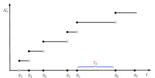
Let (Tk)k(T_{k})_{k\in{\mathbb{N}}} be a sequence of i.i.d. random variables on some probability space (Ω,,)(\Omega,{\mathcal{F}},{\mathbb{P}}) with common exponential distribution of parameter 11, i.e.,

(Tkt)=et,t0,k=1,2,.{\mathbb{P}}(T_{k}\geqslant t)=\mathrm{e}^{-t},\ \ t\geqslant 0,\ \ k=1,2,\cdots.

Let S00S_{0}\equiv 0, and for n1n\geqslant 1, define

Sn:=Sn1+Tn,S_{n}:=S_{n-1}+T_{n},

and for t0t\geqslant 0,

𝒩t:=max{n:Snt}.{\mathcal{N}}_{t}:=\max\{n:S_{n}\leqslant t\}.

Then 𝒩t{\mathcal{N}}_{t} is a standard Poisson process with intensity 11. In particular, SnS_{n} is the jump time of 𝒩t{\mathcal{N}}_{t}.

Refer to caption
Figure 1. Standard Poisson process

Note that

𝔼Tk=1,𝔼𝒩t=t,𝔼(𝒩tt)2=t.{\mathbb{E}}T_{k}=1,\ \ {\mathbb{E}}{\mathcal{N}}_{t}=t,\ \ {\mathbb{E}}({\mathcal{N}}_{t}-t)^{2}=t.

For given ε>0\varepsilon>0, we introduce

𝒩tε:=𝒩t/ε,𝒩~tε:=𝒩t/εt/ε.\displaystyle{\mathcal{N}}^{\varepsilon}_{t}:={\mathcal{N}}_{t/\varepsilon},\ \ \widetilde{\mathcal{N}}^{\varepsilon}_{t}:={\mathcal{N}}_{t/\varepsilon}-t/\varepsilon. (2.1)

Then 𝒩tε\mathcal{N}^{\varepsilon}_{t} is a Poisson process with intensity 1/ε1/\varepsilon. In this paper, we choose a sub-σ\sigma field 0\mathcal{F}_{0}\subset\mathcal{F}, which is independent of (Tk)k(T_{k})_{k\in\mathbb{N}} and therefore independent of (𝒩tε)t0(\mathcal{N}^{\varepsilon}_{t})_{t\geqslant 0}. We assume that 0\mathcal{F}_{0} is sufficiently rich so that for any μ𝒫(d)\mu\in\mathcal{P}(\mathbb{R}^{d}), there exists an 0\mathcal{F}_{0}-measurable random variable X0X_{0} such that X01=μ\mathbb{P}\circ X_{0}^{-1}=\mu. In particular, if we introduce the filtration

tε:=0σ{𝒩sε:st},t0,{\mathcal{F}}^{\varepsilon}_{t}:={\mathcal{F}}_{0}\vee\sigma\{{\mathcal{N}}^{\varepsilon}_{s}:s\leqslant t\},\ \ t\geqslant 0,

then one can verify that 𝒩~tε\widetilde{\mathcal{N}}^{\varepsilon}_{t} is an tε{\mathcal{F}}^{\varepsilon}_{t}-martingale.

In the following, we will utilize an SDE driven by Poisson process 𝒩tε\mathcal{N}^{\varepsilon}_{t} to construct a discrete approximation for ODEs. We will demonstrate the convergence of this approximation under various assumptions and establish certain functional central limit theorems.

2.1. Classical solutions for ODEs with Lipschitz coefficients

In this section, we begin by considering the case where the vector fields are bounded and Lipschitz. We demonstrate the optimal rates of strong and weak convergence for the Poisson process approximation as introduced in the introduction. Additionally, we establish a central limit theorem for this approximation scheme.

Let b:+×ddb:{\mathbb{R}}_{+}\times{\mathbb{R}}^{d}\to{\mathbb{R}}^{d} be a measurable vector field. Suppose that

b+b<,\displaystyle\|b\|_{\infty}+\|\nabla b\|_{\infty}<\infty, (2.2)

where \|\cdot\|_{\infty} is the usual LL^{\infty}-norm in +×d{\mathbb{R}}_{+}\times{\mathbb{R}}^{d}. For any 0{\mathcal{F}}_{0}-measurable initial value X0X_{0}, by the Cauchy-Lipschitz theorem, there is a unique global solution XtX_{t} to the following ODE:

Xt=X0+0tb(s,Xs)ds.\displaystyle X_{t}=X_{0}+\int^{t}_{0}b(s,X_{s}){\mathord{{\rm d}}}s. (2.3)

Let Xt(x)X_{t}(x) be the unique solution starting from xdx\in{\mathbb{R}}^{d}. Then

Xt=Xt(x)|x=X0.X_{t}=X_{t}(x)|_{x=X_{0}}.

Now we consider the following SDE driven by Poisson process 𝒩ε{\mathcal{N}}^{\varepsilon}:

Xtε=X0+0tεb(s,Xsε)d𝒩sε.\displaystyle X^{\varepsilon}_{t}=X_{0}+\int^{t}_{0}\varepsilon b(s,X^{\varepsilon}_{s-}){\mathord{{\rm d}}}{\mathcal{N}}^{\varepsilon}_{s}. (2.4)

Since s𝒩sεs\mapsto{\mathcal{N}}^{\varepsilon}_{s} is a step function (see Figure 1), it is easy to see that

Xtε=X0+εstb(s,Xsε)Δ𝒩sε=X0+εn=1b(Snε,XSn1εε)𝟙Snεt,\displaystyle X^{\varepsilon}_{t}=X_{0}+\varepsilon\sum_{s\leqslant t}b(s,X^{\varepsilon}_{s-})\Delta{\mathcal{N}}^{\varepsilon}_{s}=X_{0}+\varepsilon\sum_{n=1}^{\infty}b(S^{\varepsilon}_{n},X^{\varepsilon}_{S^{\varepsilon}_{n-1}}){\mathbbm{1}}_{S^{\varepsilon}_{n}\leqslant t},

where Δ𝒩sε:=𝒩sε𝒩sε\Delta{\mathcal{N}}^{\varepsilon}_{s}:={\mathcal{N}}^{\varepsilon}_{s}-{\mathcal{N}}^{\varepsilon}_{s-} and Snε:=εSnS^{\varepsilon}_{n}:=\varepsilon S_{n}. In particular,

XtεXtε=εb(t,Xtε)Δ𝒩tε\displaystyle X^{\varepsilon}_{t}-X^{\varepsilon}_{t-}=\varepsilon b(t,X^{\varepsilon}_{t-})\Delta{\mathcal{N}}^{\varepsilon}_{t} (2.5)

and

Xtε=X0+0tb(s,Xsε)ds+0tεb(s,Xsε)d𝒩~sε,\displaystyle X^{\varepsilon}_{t}=X_{0}+\int^{t}_{0}b(s,X^{\varepsilon}_{s}){\mathord{{\rm d}}}s+\int^{t}_{0}\varepsilon b(s,X^{\varepsilon}_{s-}){\mathord{{\rm d}}}\widetilde{\mathcal{N}}^{\varepsilon}_{s}, (2.6)

where we have used that b(s,Xsε)=b(s,Xsε)b(s,X^{\varepsilon}_{s})=b(s,X^{\varepsilon}_{s-}) except countable many points ss. It is worth noting that the solvability of the SDE (2.5) does not need any regularity assumptions on bb, and the second integral term is a martingale. In a sense, we can view (2.5) as an Euler scheme with random step sizes. Furthermore, let Xtε(x)X^{\varepsilon}_{t}(x) be the unique solution of (2.4) starting from xx. Then

Xtε=Xtε(x)|x=X0.X^{\varepsilon}_{t}=X^{\varepsilon}_{t}(x)|_{x=X_{0}}.

Hence, if X00X_{0}\in\mathcal{F}_{0} has a density, then for each t>0t>0, XtεX^{\varepsilon}_{t} also possesses a density.

First of all we show the following simple approximation result.

Theorem 2.1.
  1. (i)

    (Strong Convergence) Under (2.2), for any T>0T>0, we have

    𝔼(supt[0,T]|XtεXt|2)4e2bTb2Tε,ε(0,1).{\mathbb{E}}\left(\sup_{t\in[0,T]}|X^{\varepsilon}_{t}-X_{t}|^{2}\right)\leqslant 4\mathrm{e}^{2\|\nabla b\|_{\infty}T}\|b\|^{2}_{\infty}T\varepsilon,\ \ \varepsilon\in(0,1).
  2. (ii)

    (Weak Convergence) Under (2.2) and 2b<\|\nabla^{2}b\|_{\infty}<\infty, for any T>0T>0, there is a constant C=C(T,bCb2)>0C=C(T,\|b\|_{C^{2}_{b}})>0 such that for any ff with fCb1<\|\nabla f\|_{C^{1}_{b}}<\infty and t[0,T]t\in[0,T],

    |𝔼f(Xtε)𝔼f(Xt)|CfCb1ε,ε(0,1).|{\mathbb{E}}f(X^{\varepsilon}_{t})-{\mathbb{E}}f(X_{t})|\leqslant C\|\nabla f\|_{C^{1}_{b}}\varepsilon,\ \ \varepsilon\in(0,1).
Proof.

Noting that by (2.6) and (2.3),

XtεXt\displaystyle X^{\varepsilon}_{t}-X_{t} =0t(b(s,Xsε)b(s,Xs))ds+0tεb(s,Xsε)d𝒩~sε,\displaystyle=\int^{t}_{0}(b(s,X^{\varepsilon}_{s})-b(s,X_{s})){\mathord{{\rm d}}}s+\int^{t}_{0}\varepsilon b(s,X^{\varepsilon}_{s-}){\mathord{{\rm d}}}\widetilde{\mathcal{N}}^{\varepsilon}_{s},

we have

|XtεXt|\displaystyle|X^{\varepsilon}_{t}-X_{t}| |0t(b(s,Xsε)b(s,Xs))ds|+|0tεb(s,Xsε)d𝒩~sε|\displaystyle\leqslant\left|\int^{t}_{0}(b(s,X^{\varepsilon}_{s})-b(s,X_{s})){\mathord{{\rm d}}}s\right|+\left|\int^{t}_{0}\varepsilon b(s,X^{\varepsilon}_{s-}){\mathord{{\rm d}}}\widetilde{\mathcal{N}}^{\varepsilon}_{s}\right|
b0t|XsεXs|ds+|0tεb(s,Xsε)d𝒩~sε|.\displaystyle\leqslant\|\nabla b\|_{\infty}\int^{t}_{0}|X^{\varepsilon}_{s}-X_{s}|{\mathord{{\rm d}}}s+\left|\int^{t}_{0}\varepsilon b(s,X^{\varepsilon}_{s-}){\mathord{{\rm d}}}\widetilde{\mathcal{N}}^{\varepsilon}_{s}\right|.

Hence, by Gronwall’s inequality and Doob’s maximal inequality,

𝔼(supt[0,T]|XtεXt|2)\displaystyle{\mathbb{E}}\left(\sup_{t\in[0,T]}|X^{\varepsilon}_{t}-X_{t}|^{2}\right) e2bT𝔼(supt[0,T]|0tεb(s,Xsε)d𝒩~sε|2)\displaystyle\leqslant\mathrm{e}^{2\|\nabla b\|_{\infty}T}{\mathbb{E}}\left(\sup_{t\in[0,T]}\left|\int^{t}_{0}\varepsilon b(s,X^{\varepsilon}_{s-}){\mathord{{\rm d}}}\widetilde{\mathcal{N}}^{\varepsilon}_{s}\right|^{2}\right)
4e2bT𝔼|0Tεb(s,Xsε)d𝒩~sε|2\displaystyle\leqslant 4\mathrm{e}^{2\|\nabla b\|_{\infty}T}{\mathbb{E}}\left|\int^{T}_{0}\varepsilon b(s,X^{\varepsilon}_{s-}){\mathord{{\rm d}}}\widetilde{\mathcal{N}}^{\varepsilon}_{s}\right|^{2}
=4e2bT𝔼(0T|εb(s,Xsε)|2d(sε))\displaystyle=4\mathrm{e}^{2\|\nabla b\|_{\infty}T}{\mathbb{E}}\left(\int^{T}_{0}|\varepsilon b(s,X^{\varepsilon}_{s})|^{2}{\mathord{{\rm d}}}{\big{(}}\tfrac{s}{\varepsilon}{\big{)}}\right)
4e2bTb2Tε.\displaystyle\leqslant 4\mathrm{e}^{2\|\nabla b\|_{\infty}T}\|b\|^{2}_{\infty}T\varepsilon.

(ii) Fix t>0t>0 and fCb2(d)f\in C^{2}_{b}({\mathbb{R}}^{d}). Let u(s,x)u(s,x) solve the backward transport equation:

su+bu=0,u(t,x)=f(x).\displaystyle\partial_{s}u+b\cdot\nabla u=0,\ \ u(t,x)=f(x). (2.7)

In fact, the unique solution of the above transport equation is given by

u(s,x)=f(Xs,t(x)),u(s,x)=f(X_{s,t}(x)),

where Xs,t(x)X_{s,t}(x) solves the following ODE:

Xs,t(x)=x+stb(r,Xs,r(x))dr.X_{s,t}(x)=x+\int^{t}_{s}b(r,X_{s,r}(x)){\mathord{{\rm d}}}r.

Since b,f\nabla b,\nabla f, 2b,2fL\nabla^{2}b,\nabla^{2}f\in L^{\infty}, by the chain rule, it is easy to derive that

2u(s,)\displaystyle\|\nabla^{2}u(s,\cdot)\|_{\infty} 2fXs,t2+f2Xs,t\displaystyle\leqslant\|\nabla^{2}f\|_{\infty}\|\nabla X_{s,t}\|_{\infty}^{2}+\|\nabla f\|_{\infty}\|\nabla^{2}X_{s,t}\|_{\infty}
e4b(ts)(2f+f2b),\displaystyle\leqslant\mathrm{e}^{4\|\nabla b\|_{\infty}(t-s)}\Big{(}\|\nabla^{2}f\|_{\infty}+\|\nabla f\|_{\infty}\|\nabla^{2}b\|_{\infty}\Big{)},

and for the solution XtX_{t} of (2.3),

f(Xt)=u(t,Xt)=u(0,X0)+0t(su+bu)(s,Xs)ds=u(0,X0).\displaystyle f(X_{t})=u(t,X_{t})=u(0,X_{0})+\int^{t}_{0}(\partial_{s}u+b\cdot\nabla u)(s,X_{s}){\mathord{{\rm d}}}s=u(0,X_{0}). (2.8)

Moreover, by Itô’s formula we have

𝔼f(Xtε)=𝔼u(t,Xtε)=𝔼u(0,X0)+𝔼0t[su(s,Xsε)+u(s,Xsε+εb(s,Xsε))u(s,Xsε)ε]ds.\displaystyle{\mathbb{E}}f(X^{\varepsilon}_{t})={\mathbb{E}}u(t,X^{\varepsilon}_{t})={\mathbb{E}}u(0,X_{0})+{\mathbb{E}}\int^{t}_{0}\left[\partial_{s}u(s,X^{\varepsilon}_{s})+\frac{u(s,X^{\varepsilon}_{s}+\varepsilon b(s,X^{\varepsilon}_{s}))-u(s,X^{\varepsilon}_{s})}{\varepsilon}\right]{\mathord{{\rm d}}}s.

Hence, by (2.7) and (2.8),

|𝔼f(Xtε)𝔼f(Xt)|\displaystyle|{\mathbb{E}}f(X^{\varepsilon}_{t})-{\mathbb{E}}f(X_{t})| =|𝔼0tb(s,Xsε)01(u(s,Xsε+θεb(s,Xsε))u(s,Xsε))dθds|\displaystyle=\left|{\mathbb{E}}\int^{t}_{0}b(s,X^{\varepsilon}_{s})\cdot\int^{1}_{0}\Big{(}\nabla u(s,X^{\varepsilon}_{s}+\theta\varepsilon b(s,X^{\varepsilon}_{s}))-\nabla u(s,X^{\varepsilon}_{s})\Big{)}{\mathord{{\rm d}}}\theta{\mathord{{\rm d}}}s\right|
b22uε01θdθb2e4bt(2f+f2b)ε2.\displaystyle\leqslant\|b\|^{2}_{\infty}\|\nabla^{2}u\|_{\infty}\varepsilon\int^{1}_{0}\theta{\mathord{{\rm d}}}\theta\leqslant\|b\|^{2}_{\infty}\mathrm{e}^{4\|\nabla b\|_{\infty}t}\Big{(}\|\nabla^{2}f\|_{\infty}+\|\nabla f\|_{\infty}\|\nabla^{2}b\|_{\infty}\Big{)}\tfrac{\varepsilon}{2}.

The proof is complete. ∎

Remark 2.2.

It is noted that the rate of weak convergence is better than the rate of strong convergence in the Poisson process approximation. The order of convergence, both in terms of strong and weak convergence, is the same as the classical Euler approximation of SDEs (see [25]).

Remark 2.3.

Consider a measurable function ff . For ε>0\varepsilon>0, let us define

Ifε(t):=ε0tf(s)d𝒩sε=εstf(s)Δ𝒩sε.I^{\varepsilon}_{f}(t):=\varepsilon\int^{t}_{0}f(s){\mathord{{\rm d}}}{\mathcal{N}}^{\varepsilon}_{s}=\varepsilon\sum_{s\leqslant t}f(s)\Delta{\mathcal{N}}^{\varepsilon}_{s}.

By applying Doob’s maximal inequality, we obtain

𝔼[supt[0,T]|Ifε(t)0tf(s)ds|2]4ε0T|f(s)|2ds.{\mathbb{E}}\left[\sup_{t\in[0,T]}\left|I^{\varepsilon}_{f}(t)-\int^{t}_{0}f(s){\mathord{{\rm d}}}s\right|^{2}\right]\leqslant 4\varepsilon\int^{T}_{0}|f(s)|^{2}{\mathord{{\rm d}}}s.

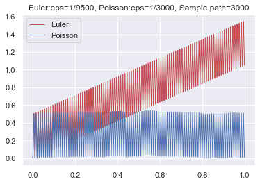
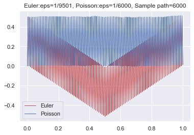
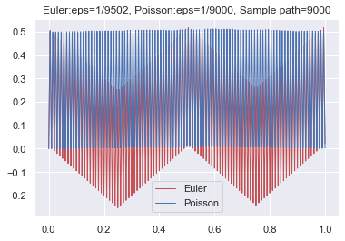
It is worth noting that the calculation of Ifε(t)I^{\varepsilon}_{f}(t) can be easily implemented on a computer, where the step size is randomly chosen according to the exponential distribution. As a result, we can utilize the Monte Carlo method to theoretically compute the integral 0Tf(s)ds\int_{0}^{T}f(s)\mathrm{d}s. To illustrate the effectiveness of our scheme, we provide an example involving a highly oscillatory function:

f(s):=(12([200s]%2))100,s[0,1],f(s):=(1-2*([200*s]\%2))*100,\ \ s\in[0,1],

where [a][a] stands for the integer part of aa and n%2=1n\%2=1 or 0 depends on nn being odd or even. Note that t0tf(s)ds=:F(t)t\mapsto\int^{t}_{0}f(s){\mathord{{\rm d}}}s=:F(t) oscillates between 0 and 0.50.5. We simulate the graph using both Euler’s scheme and the Poisson approximation scheme, as depicted in Figure 2. From the graph, we can observe that Euler’s scheme exhibits instability due to the regular choice of partition points. Conversely, Poisson’s scheme demonstrates stability, with partition points being chosen randomly.

Refer to caption
Refer to caption
Refer to caption
Figure 2. Comparison between Euler scheme and Poisson scheme

Next, we investigate the asymptotic distribution of the following deviation as ε0\varepsilon\to 0,

Ztε:=XtεXtε.Z^{\varepsilon}_{t}:=\frac{X^{\varepsilon}_{t}-X_{t}}{\sqrt{\varepsilon}}.

By (2.4) and (2.6), it is easy to see that

Ztε=0tεb(s,Xsε)d𝒩~sε+0tb(Xsε)b(Xs)εds=0tεb(s,Xsε)d𝒩~sε+0tZsεBsεds,\displaystyle\begin{split}Z_{t}^{\varepsilon}&=\int^{t}_{0}\sqrt{\varepsilon}b(s,X^{\varepsilon}_{s-}){\mathord{{\rm d}}}\widetilde{\mathcal{N}}^{\varepsilon}_{s}+\int^{t}_{0}\frac{b(X^{\varepsilon}_{s})-b(X_{s})}{\sqrt{\varepsilon}}{\mathord{{\rm d}}}s\\ &=\int^{t}_{0}\sqrt{\varepsilon}b(s,X^{\varepsilon}_{s-}){\mathord{{\rm d}}}\widetilde{\mathcal{N}}^{\varepsilon}_{s}+\int^{t}_{0}Z^{\varepsilon}_{s}B^{\varepsilon}_{s}{\mathord{{\rm d}}}s,\end{split} (2.9)

where

Bsε:=01b(s,θXsε+(1θ)Xs)dθ=01b(s,Xs+εθZsε)dθ.B^{\varepsilon}_{s}:=\int^{1}_{0}\nabla b(s,\theta X^{\varepsilon}_{s}+(1-\theta)X_{s}){\mathord{{\rm d}}}\theta=\int^{1}_{0}\nabla b(s,X_{s}+\sqrt{\varepsilon}\theta Z^{\varepsilon}_{s}){\mathord{{\rm d}}}\theta.

Note that as ε0\varepsilon\to 0,

𝔼eiξε𝒩~tε=exp{tε1(eiξε1)iξt/ε}eξ2t/2.{\mathbb{E}}\mathrm{e}^{{\rm i}\xi\sqrt{\varepsilon}\widetilde{\mathcal{N}}^{\varepsilon}_{t}}=\exp\big{\{}t\varepsilon^{-1}(\mathrm{e}^{{\rm i}\xi\sqrt{\varepsilon}}-1)-{\rm i}\xi t/\sqrt{\varepsilon}\big{\}}\to\mathrm{e}^{-\xi^{2}t/2}.

This implies that ε𝒩~tε\sqrt{\varepsilon}\widetilde{\mathcal{N}}^{\varepsilon}_{t} weakly converges to a one-dimensional standard Brownian motion WtW_{t}. Therefore, we formally have ZεZZ^{\varepsilon}\Rightarrow Z, where ZZ solves the following linear SDE:

Zt=0tb(s,Xs)dWs+0tZsb(s,Xs)ds.\displaystyle Z_{t}=\int^{t}_{0}b(s,X_{s}){\mathord{{\rm d}}}W_{s}+\int^{t}_{0}Z_{s}\cdot\nabla b(s,X_{s}){\mathord{{\rm d}}}s. (2.10)

Clearly, ZtZ_{t} is an OU process and it’s infinitesimal generator is given by

sf(z)=12tr((bb)(s,Xs)2f(z))+zb(s,Xs),f(z).\displaystyle{\mathscr{L}}_{s}f(z)=\tfrac{1}{2}\mathrm{tr}{\big{(}}(b\otimes b)(s,X_{s})\cdot\nabla^{2}f(z){\big{)}}+\langle z\cdot\nabla b(s,X_{s}),\nabla f(z)\rangle. (2.11)
Proposition 2.4.

Let {\mathscr{L}} be given in (2.11) with bb being a bounded Lipschitz vector field. For any (s,z)+×d(s,z)\in{\mathbb{R}}_{+}\times{\mathbb{R}}^{d}, there is a unique martingale solution sz(){\mathbb{P}}\in{\mathcal{M}}^{z}_{s}({\mathscr{L}}) in the sense of Definition 6.2 in the appendix. Moreover, {\mathbb{P}} concentrates on the space of continuous functions.

Proof.

Since the diffusion coefficient does not depend on zz and the drift is linear in zz, it is easy to see that for any (s,z)+×d(s,z)\in{\mathbb{R}}_{+}\times{\mathbb{R}}^{d}, there is a unique martingale solution s,zsz(){\mathbb{P}}_{s,z}\in{\mathcal{M}}^{z}_{s}({\mathscr{L}}). Moreover, by Proposition 6.3 in appendix, {\mathbb{P}} concentrates on the space of continuous functions. ∎

Now we show the following functional CLT about the above ZεZ^{\varepsilon}.

Theorem 2.5.

Suppose that bb is bounded and Lipschitz continuous. Let 00(){\mathbb{P}}\in{\mathcal{M}}^{0}_{0}({\mathscr{L}}) be the unique martingale solution associated with {\mathscr{L}} starting from 0 at time 0. Let ε{\mathbb{P}}_{\varepsilon} be the law of Zε:=XεXεZ^{\varepsilon}:=\frac{X^{\varepsilon}-X}{\sqrt{\varepsilon}} in the space 𝔻{\mathbb{D}} of càdlàg functions, where XεX^{\varepsilon} is the unique solution of SDE (2.4) with the same fixed initial value X0=x0X_{0}=x_{0} as XX. Then we have

ε in 𝒫(𝔻).{\mathbb{P}}_{\varepsilon}\Rightarrow{\mathbb{P}}\mbox{ in ${\mathcal{P}}({\mathbb{D}})$}.
Proof.

First of all, for any fCb2(d)f\in C^{2}_{b}({\mathbb{R}}^{d}), by (2.9) and Itô’s formula, we have

f(Ztε)=f(0)+0t[Asεf(Zsε)+(ZsεBsε)f(Zsε)]ds+Mtε,\displaystyle f(Z^{\varepsilon}_{t})=f(0)+\int^{t}_{0}\Big{[}A^{\varepsilon}_{s}f(Z^{\varepsilon}_{s})+(Z^{\varepsilon}_{s}B^{\varepsilon}_{s})\cdot\nabla f(Z^{\varepsilon}_{s})\Big{]}{\mathord{{\rm d}}}s+M^{\varepsilon}_{t},

where Mtε:=0t(f(Zsε+εb(s,Xsε))f(Zsε))d𝒩~sεM^{\varepsilon}_{t}:=\int^{t}_{0}\big{(}f(Z^{\varepsilon}_{s-}+\sqrt{\varepsilon}b(s,X^{\varepsilon}_{s-}))-f(Z^{\varepsilon}_{s-})\big{)}{\mathord{{\rm d}}}\widetilde{\mathcal{N}}^{\varepsilon}_{s} is a martingale and

Asεf(z)=f(z+εb(s,Xs))f(z)εb(s,Xs)f(z)ε.\displaystyle A^{\varepsilon}_{s}f(z)=\frac{f(z+\sqrt{\varepsilon}b(s,X_{s}))-f(z)-\sqrt{\varepsilon}b(s,X_{s})\cdot\nabla f(z)}{\varepsilon}.

Therefore, the infinitesimal generator of ZtεZ^{\varepsilon}_{t} is given by

s(ε)f(z):=Asεf(z)+(zBsε)f(z).{\mathscr{L}}^{(\varepsilon)}_{s}f(z):=A^{\varepsilon}_{s}f(z)+(zB^{\varepsilon}_{s})\cdot\nabla f(z).

From the very definition, it is easy to see that for any s,R>0s,R>0,

limε0sup|z|R|s(ε)f(z)sf(z)|=0.\displaystyle\lim_{\varepsilon\to 0}\sup_{|z|\leqslant R}|{\mathscr{L}}^{(\varepsilon)}_{s}f(z)-{\mathscr{L}}_{s}f(z)|=0. (2.12)

In fact, noting that by Taylor’s expansion,

Asεf(z)=01θ01tr((bb)(s,Xs)2f(z+θθεb(s,Xs))dθdθ,A^{\varepsilon}_{s}f(z)=\int^{1}_{0}\theta\int^{1}_{0}\mathrm{tr}\Big{(}(b\otimes b)(s,X_{s})\cdot\nabla^{2}f(z+\theta\theta^{\prime}\sqrt{\varepsilon}b(s,X_{s})\Big{)}{\mathord{{\rm d}}}\theta{\mathord{{\rm d}}}\theta^{\prime},

one sees that for each s>0s>0,

limε0sup|z|R|Asεf(z)12tr((bb)(s,Xs)2f(z))|=0.\displaystyle\lim_{\varepsilon\to 0}\sup_{|z|\leqslant R}\Big{|}A^{\varepsilon}_{s}f(z)-\tfrac{1}{2}\mathrm{tr}{\big{(}}(b\otimes b)(s,X_{s})\cdot\nabla^{2}f(z){\big{)}}\Big{|}=0.

Moreover, by the definition of BsεB^{\varepsilon}_{s}, we clearly have

limε0|Bsεb(s,Xs)|=0.\lim_{\varepsilon\to 0}|B^{\varepsilon}_{s}-\nabla b(s,X_{s})|=0.

Thus we have (2.12). On the other hand, by (2.9) and Gronwall’s lemma, it is easy to see that for some C>0C>0,

supε(0,1)𝔼(supt[0,T]|Ztε|2)C,\sup_{\varepsilon\in(0,1)}{\mathbb{E}}\left(\sup_{t\in[0,T]}|Z_{t}^{\varepsilon}|^{2}\right)\leqslant C,

and for any stopping time τ\tau and δ>0\delta>0,

supε(0,1)𝔼(supt[0,δ]|Zτ+tεZτε|2)Cδ.\displaystyle\sup_{\varepsilon\in(0,1)}{\mathbb{E}}\left(\sup_{t\in[0,\delta]}|Z^{\varepsilon}_{\tau+t}-Z^{\varepsilon}_{\tau}|^{2}\right)\leqslant C\delta.

Thus, by Aldous’ criterion (see [23, p356, Theorem 4.5]), (ε)ε(0,1)({\mathbb{P}}_{\varepsilon})_{\varepsilon\in(0,1)} is tight. Let 0{\mathbb{P}}_{0} be any accumulation point. By (2.12) and Theorem 6.4 in appendix, 000(){\mathbb{P}}_{0}\in{\mathcal{M}}^{0}_{0}({\mathscr{L}}). By the uniqueness (see Proposition 2.4), one has 0={\mathbb{P}}_{0}={\mathbb{P}}. The proof is complete. ∎

Remark 2.6.

We emphasize that in the above theorem, the initial value is a nonrandom fixed point. We shall consider the general random initial value in Theorem 2.19 below.

2.2. Filippov solutions for ODEs with one-sided Lipschitz coefficients

In this section, our focus is on the Poisson process approximation for the ODE (2.3) with one-sided Lipschitz coefficients. We will explore the convergence properties and effectiveness of this approximation scheme in this setting.

  1. (Hb)

    We assume that for some κ>0\kappa>0 and all (s,x,y)+×d×d(s,x,y)\in{\mathbb{R}}_{+}\times{\mathbb{R}}^{d}\times{\mathbb{R}}^{d},

    xy,b(s,x)b(s,y)κ|xy|2,|b(s,x)|κ(1+|x|).\langle x-y,b(s,x)-b(s,y)\rangle\leqslant\kappa|x-y|^{2},\ \ |b(s,x)|\leqslant\kappa(1+|x|).

Due to the lack of continuity of xb(s,x)x\mapsto b(s,x), assumption (Hb) does not guarantee the existence of a solution to the ODE (2.3) in the classical sense. In such cases, Filippov [14] introduced a concept of solution in the sense of differential inclusions, providing a unique solution to the ODE (2.3). This notion is closely connected to the study of differential inclusions as discussed in [2].

To define Filippov solutions, we introduce the supporting function HbH_{b} of bb, defined by

Hb(t,x,w):=limδ0esssup|yx|δb(t,y),w,H_{b}(t,x,w):=\lim_{\delta\downarrow 0}{\rm ess}\!\!\!\!\!\sup_{|y-x|\leqslant\delta}\langle b(t,y),w\rangle,

where the essential supremum is taken with respect to the Lebesgue measure. The essential convex hull of bb is then given by

At,xb:={yd:y,wHb(t,x,w),wd}.A^{b}_{t,x}:=\{y\in{\mathbb{R}}^{d}:\langle y,w\rangle\leqslant H_{b}(t,x,w),w\in{\mathbb{R}}^{d}\}.

Note that At,xbA^{b}_{t,x} is a closed convex subset and Hb(t,x,)H_{b}(t,x,\cdot) is precisely the support function of At,xbA^{b}_{t,x}.

Definition 2.7.

We call an absolutely continuous curve (Xt)t0(X_{t})_{t\geqslant 0} in d{\mathbb{R}}^{d} a Filippov solution of ODE (2.3) starting from x0x_{0} if X0=x0X_{0}=x_{0} and for Lebesgue almost all t0t\geqslant 0,

X˙tAt,Xtb.\dot{X}_{t}\in A^{b}_{t,X_{t}}.

In [14], Filippov proved the following result (see also [20, Theorem 1.42]) .

Theorem 2.8.

Under (Hb), for any starting point X0=x0X_{0}=x_{0}, there is a unique Filippov solution (Xt(x0))t0(X_{t}(x_{0}))_{t\geqslant 0} to ODE (2.3). Moreover, for any x0,x0dx_{0},x_{0}^{\prime}\in{\mathbb{R}}^{d} and t0t\geqslant 0,

|Xt(x0)Xt(x0)|e2κt|x0x0|.\displaystyle|X_{t}(x_{0})-X_{t}(x^{\prime}_{0})|\leqslant\mathrm{e}^{2\kappa t}|x_{0}-x_{0}^{\prime}|. (2.13)

Let bδ(t,x):=b(t,)ρδ(x)b_{\delta}(t,x):=b(t,\cdot)*\rho_{\delta}(x) be the mollifier approximation of bb, where ρδ(x)=δdρ(x/δ)\rho_{\delta}(x)=\delta^{-d}\rho(x/\delta) and ρ\rho is a smooth density function with compact support. Let Xδ(x0)X^{\delta}(x_{0}) be the unique solution of ODE (2.3) corresponding to bδb_{\delta} and starting from x0x_{0}. Then for any T>0T>0, we have

limδ0supt[0,T]|Xtδ(x0)Xt(x0)|=0.\displaystyle\lim_{\delta\to 0}\sup_{t\in[0,T]}|X^{\delta}_{t}(x_{0})-X_{t}(x_{0})|=0. (2.14)

The existence of a Filippov solution can be established through a compactness argument, while the uniqueness follows from the one-sided Lipschitz condition. It is remarkable that we can show that the Filippov solution of the ODE (2.3) coincides with the LpL^{p}-limit of XεX^{\varepsilon} under assumption (Hb). This result is particularly significant as it provides an explicit time discretization scheme for Filippov solutions. To prove this result, we begin by demonstrating a simple convergence estimate in the case where bb is continuous in xx.

Lemma 2.9.

Let X0ε=ξp>1Lp(Ω,0,)X^{\varepsilon}_{0}=\xi\in\cap_{p>1}L^{p}(\Omega,{\mathcal{F}}_{0},{\mathbb{P}}). Suppose that (Hb) and for each t0t\geqslant 0, xb(t,x)x\mapsto b(t,x) is continuous. Then for any T>0T>0 and p1p\geqslant 1, there is a constant C=C(κ,d,T,p)>0C=C(\kappa,d,T,p)>0 such that

supε(0,1)𝔼(supt[0,T]|Xtε|p)C(1+𝔼|ξ|p),\displaystyle\sup_{\varepsilon\in(0,1)}{\mathbb{E}}\left(\sup_{t\in[0,T]}|X^{\varepsilon}_{t}|^{p}\right)\leqslant C(1+{\mathbb{E}}|\xi|^{p}), (2.15)

and for all ε(0,1)\varepsilon\in(0,1),

𝔼(supt[0,T]|XtεXt|2p)C(1+𝔼|ξ|2p)εp,\displaystyle{\mathbb{E}}\left(\sup_{t\in[0,T]}|X^{\varepsilon}_{t}-X_{t}|^{2p}\right)\leqslant C(1+{\mathbb{E}}|\xi|^{2p})\varepsilon^{p}, (2.16)

where XX is the unique solution of ODE (2.3) starting from ξ\xi.

Proof.

For p1p\geqslant 1, by Itô’s formula and |x+y|p|x|pp|y|(|x|+|y|)p1|x+y|^{p}-|x|^{p}\leqslant p|y|(|x|+|y|)^{p-1}, we have

|Xtε|p\displaystyle|X^{\varepsilon}_{t}|^{p} =|ξ|p+0t(|Xsε+εb(s,Xsε)|p|Xsε|p)d𝒩sε\displaystyle=|\xi|^{p}+\int^{t}_{0}(|X^{\varepsilon}_{s-}+\varepsilon b(s,X^{\varepsilon}_{s-})|^{p}-|X^{\varepsilon}_{s-}|^{p}){\mathord{{\rm d}}}{\mathcal{N}}^{\varepsilon}_{s}
|ξ|p+pε0t|b(s,Xsε)|(|Xsε|+ε|b(s,Xsε)|)p1d𝒩sε.\displaystyle\leqslant|\xi|^{p}+p\varepsilon\int^{t}_{0}|b(s,X^{\varepsilon}_{s-})|\big{(}|X^{\varepsilon}_{s-}|+\varepsilon|b(s,X^{\varepsilon}_{s-})|\big{)}^{p-1}{\mathord{{\rm d}}}{\mathcal{N}}^{\varepsilon}_{s}.

Hence, by the linear growth of bb in xx,

𝔼(sups[0,t]|Xsε|p)\displaystyle{\mathbb{E}}\left(\sup_{s\in[0,t]}|X^{\varepsilon}_{s}|^{p}\right) 𝔼|ξ|p+pε𝔼(0t|b(s,Xsε)|(|Xsε|+ε|b(s,Xsε)|)p1d𝒩sε)\displaystyle\leqslant{\mathbb{E}}|\xi|^{p}+p\varepsilon{\mathbb{E}}\left(\int^{t}_{0}|b(s,X^{\varepsilon}_{s})|\big{(}|X^{\varepsilon}_{s}|+\varepsilon|b(s,X^{\varepsilon}_{s})|\big{)}^{p-1}{\mathord{{\rm d}}}{\mathcal{N}}^{\varepsilon}_{s}\right)
=𝔼|ξ|p+p𝔼(0t|b(s,Xsε)|(|Xsε|+ε|b(s,Xsε)|)p1ds)\displaystyle={\mathbb{E}}|\xi|^{p}+p{\mathbb{E}}\left(\int^{t}_{0}|b(s,X^{\varepsilon}_{s})|\big{(}|X^{\varepsilon}_{s}|+\varepsilon|b(s,X^{\varepsilon}_{s})|\big{)}^{p-1}{\mathord{{\rm d}}}s\right)
𝔼|ξ|p+C𝔼(0t(1+|Xsε|p)ds),\displaystyle\leqslant{\mathbb{E}}|\xi|^{p}+C{\mathbb{E}}\left(\int^{t}_{0}(1+|X^{\varepsilon}_{s}|^{p}){\mathord{{\rm d}}}s\right),

which implies the first estimate by Gronwall’s inequality.

Next, we look at (2.16). Since b(t,x)b(t,x) is continuous in xx for each t>0t>0, it is well-known that there is a unique classical solution to ODE (2.3) under (Hb). Note that

Zt:=XtεXt=0tεb(s,Xsε)d𝒩~sε+0t[b(s,Xsε)b(s,Xs)]ds.Z_{t}:=X^{\varepsilon}_{t}-X_{t}=\int^{t}_{0}\varepsilon b(s,X^{\varepsilon}_{s-}){\mathord{{\rm d}}}\widetilde{\mathcal{N}}^{\varepsilon}_{s}+\int^{t}_{0}\Big{[}b(s,X^{\varepsilon}_{s})-b(s,X_{s})\Big{]}{\mathord{{\rm d}}}s.

By Itô’s formula and (Hb), we have

|Ztε|2\displaystyle|Z^{\varepsilon}_{t}|^{2} =20tZsε,b(s,Xsε)b(s,Xs)ds+0t(|Zsε+εb(s,Xsε)|2|Zsε|2)d𝒩~sε\displaystyle=2\int^{t}_{0}\langle Z^{\varepsilon}_{s},b(s,X^{\varepsilon}_{s})-b(s,X_{s})\rangle{\mathord{{\rm d}}}s+\int^{t}_{0}(|Z^{\varepsilon}_{s-}+\varepsilon b(s,X^{\varepsilon}_{s-})|^{2}-|Z^{\varepsilon}_{s-}|^{2}){\mathord{{\rm d}}}\widetilde{\mathcal{N}}^{\varepsilon}_{s}
+0t(|Zsε+εb(s,Xsε)|2|Zsε|22εb(s,Xsε),Zsε)d(sε)\displaystyle\quad+\int^{t}_{0}(|Z^{\varepsilon}_{s}+\varepsilon b(s,X^{\varepsilon}_{s})|^{2}-|Z^{\varepsilon}_{s}|^{2}-2\varepsilon\langle b(s,X^{\varepsilon}_{s}),Z^{\varepsilon}_{s}\rangle){\mathord{{\rm d}}}{\big{(}}\frac{s}{\varepsilon}{\big{)}}
2κ0t|Zsε|2ds+0t(2εb(s,Xsε),Zsε+ε2|b(s,Xsε)|2)d𝒩~sε+ε0t|b(s,Xsε)|2ds.\displaystyle\leqslant 2\kappa\int^{t}_{0}|Z^{\varepsilon}_{s}|^{2}{\mathord{{\rm d}}}s+\int^{t}_{0}\Big{(}2\varepsilon\langle b(s,X^{\varepsilon}_{s-}),Z^{\varepsilon}_{s-}\rangle+\varepsilon^{2}|b(s,X^{\varepsilon}_{s-})|^{2}\Big{)}{\mathord{{\rm d}}}\widetilde{\mathcal{N}}^{\varepsilon}_{s}+\varepsilon\int^{t}_{0}|b(s,X^{\varepsilon}_{s})|^{2}{\mathord{{\rm d}}}s.

Hence, by Gronwall’s inequality, (2.15) and BDG’s inequality, we get for p2p\geqslant 2,

𝔼(sups[0,t]|Zsε|2p)\displaystyle{\mathbb{E}}\left(\sup_{s\in[0,t]}|Z^{\varepsilon}_{s}|^{2p}\right) 𝔼|0t(2εb(s,Xsε),Zsε+ε2|b(s,Xsε)|2)d𝒩~sε|p+(1+𝔼|ξ|2p)εp\displaystyle\lesssim{\mathbb{E}}\left|\int^{t}_{0}\Big{(}2\varepsilon\langle b(s,X^{\varepsilon}_{s-}),Z^{\varepsilon}_{s-}\rangle+\varepsilon^{2}|b(s,X^{\varepsilon}_{s-})|^{2}\Big{)}{\mathord{{\rm d}}}\widetilde{\mathcal{N}}^{\varepsilon}_{s}\right|^{p}+(1+{\mathbb{E}}|\xi|^{2p})\varepsilon^{p}
𝔼(0t|2εb(s,Xsε),Zsε+ε2|b(s,Xsε)|2|2d(sε))p2\displaystyle\lesssim{\mathbb{E}}\left(\int^{t}_{0}\Big{|}2\varepsilon\langle b(s,X^{\varepsilon}_{s}),Z^{\varepsilon}_{s}\rangle+\varepsilon^{2}|b(s,X^{\varepsilon}_{s})|^{2}\Big{|}^{2}{\mathord{{\rm d}}}(\tfrac{s}{\varepsilon})\right)^{\frac{p}{2}}
+𝔼0t|2εb(s,Xsε),Zsε+ε2|b(s,Xsε)|2|pd(sε)+(1+𝔼|ξ|2p)εp\displaystyle+{\mathbb{E}}\int^{t}_{0}\Big{|}2\varepsilon\langle b(s,X^{\varepsilon}_{s}),Z^{\varepsilon}_{s}\rangle+\varepsilon^{2}|b(s,X^{\varepsilon}_{s})|^{2}\Big{|}^{p}{\mathord{{\rm d}}}(\tfrac{s}{\varepsilon})+(1+{\mathbb{E}}|\xi|^{2p})\varepsilon^{p}
𝔼(0t(|Zsε|4+ε2(1+|Xsε|4)ds)p2\displaystyle\lesssim{\mathbb{E}}\left(\int^{t}_{0}\Big{(}|Z^{\varepsilon}_{s}|^{4}+\varepsilon^{2}(1+|X^{\varepsilon}_{s}|^{4}\Big{)}{\mathord{{\rm d}}}s\right)^{\frac{p}{2}}
+𝔼0t(|Zsε|2+ε2(1+|Xsε|2)pd(sε)+(1+𝔼|ξ|2p)εp\displaystyle+{\mathbb{E}}\int^{t}_{0}\Big{(}|Z^{\varepsilon}_{s}|^{2}+\varepsilon^{2}(1+|X^{\varepsilon}_{s}|^{2}\Big{)}^{p}{\mathord{{\rm d}}}(\tfrac{s}{\varepsilon})+(1+{\mathbb{E}}|\xi|^{2p})\varepsilon^{p}
0t𝔼|Zsε|2pds+(1+𝔼|ξ|2p)εp,\displaystyle\lesssim\int^{t}_{0}{\mathbb{E}}|Z^{\varepsilon}_{s}|^{2p}{\mathord{{\rm d}}}s+(1+{\mathbb{E}}|\xi|^{2p})\varepsilon^{p},

which in turn implies the desired estimate (2.16). ∎

Next we show the continuous dependence of XεX^{\varepsilon} with respect to bb and the initial values.

Lemma 2.10.

(i) Let X0ε=ξp>1Lp(Ω,0,)X^{\varepsilon}_{0}=\xi\in\cap_{p>1}L^{p}(\Omega,{\mathcal{F}}_{0},{\mathbb{P}}) and Xε,δX^{\varepsilon,\delta} be the solution of ODE (2.4) corresponding to bδb_{\delta}, where bδb_{\delta} is the smooth approximation of bb as in Theorem 2.8. Suppose (Hb) and ξ\xi has a density with respect to the Lebesgue measure. Then for any T>0T>0 and p1p\geqslant 1, there is a constant C=C(κ,d,T,p)>0C=C(\kappa,d,T,p)>0 such that for all ε(0,1)\varepsilon\in(0,1),

limδ0𝔼(supt[0,T]|Xtε,δXtε|2p)C(1+𝔼|ξ|2p)εp.\displaystyle\lim_{\delta\to 0}{\mathbb{E}}\left(\sup_{t\in[0,T]}|X^{\varepsilon,\delta}_{t}-X^{\varepsilon}_{t}|^{2p}\right)\leqslant C(1+{\mathbb{E}}|\xi|^{2p})\varepsilon^{p}. (2.17)

(ii) Let ξ,ξ~p>1Lp(Ω,0,)\xi,\widetilde{\xi}\in\cap_{p>1}L^{p}(\Omega,{\mathcal{F}}_{0},{\mathbb{P}}) and XεX^{\varepsilon}, X~ε\widetilde{X}^{\varepsilon} be the solutions of ODE (2.4) corresponding to initial values ξ\xi and ξ~\widetilde{\xi}, respectively. Under (Hb), for any T>0T>0 and p1p\geqslant 1, there is a constant C=C(κ,d,T,p)>0C=C(\kappa,d,T,p)>0 such that for all ε(0,1)\varepsilon\in(0,1),

𝔼(supt[0,T]|XtεX~tε|2p)C𝔼|ξξ~|2p+C(1+𝔼|ξ|2p+𝔼|ξ~|2p)εp.\displaystyle{\mathbb{E}}\left(\sup_{t\in[0,T]}|X^{\varepsilon}_{t}-\tilde{X}^{\varepsilon}_{t}|^{2p}\right)\leqslant C{\mathbb{E}}|\xi-\widetilde{\xi}|^{2p}+C(1+{\mathbb{E}}|\xi|^{2p}+{\mathbb{E}}|\widetilde{\xi}|^{2p})\varepsilon^{p}. (2.18)
Proof.

We will only prove (i) since (ii) follows in the same manner. Note that

Zt:=Xtε,δXtε\displaystyle Z_{t}:=X^{\varepsilon,\delta}_{t}-X^{\varepsilon}_{t} =0tε(bδ(s,Xsε,δ)b(s,Xsε))d𝒩sε=0t[εBsε,δ+εgsδ(Xsε)]d𝒩sε,\displaystyle=\int^{t}_{0}\varepsilon(b_{\delta}(s,X^{\varepsilon,\delta}_{s-})-b(s,X^{\varepsilon}_{s-})){\mathord{{\rm d}}}{\mathcal{N}}^{\varepsilon}_{s}=\int^{t}_{0}\Big{[}\varepsilon B^{\varepsilon,\delta}_{s}+\varepsilon g^{\delta}_{s}(X^{\varepsilon}_{s-})\Big{]}{\mathord{{\rm d}}}{\mathcal{N}}^{\varepsilon}_{s},

where

Bsε,δ:=bδ(s,Xsε,δ)bδ(s,Xsε),gsδ(x):=(bδb)(s,x).B^{\varepsilon,\delta}_{s}:=b_{\delta}(s,X^{\varepsilon,\delta}_{s-})-b_{\delta}(s,X^{\varepsilon}_{s-}),\ \ g^{\delta}_{s}(x):=(b_{\delta}-b)(s,x).

By Itô’s formula and (Hb), we have

|Zt|2\displaystyle|Z_{t}|^{2} =0t(|Zs+εBsε,δ+εgsδ(Xsε)|2|Zs|2)d𝒩sε\displaystyle=\int^{t}_{0}(|Z_{s-}+\varepsilon B^{\varepsilon,\delta}_{s}+\varepsilon g^{\delta}_{s}(X^{\varepsilon}_{s-})|^{2}-|Z_{s-}|^{2}){\mathord{{\rm d}}}{\mathcal{N}}^{\varepsilon}_{s}
=0t(2εBsε,δ+gsδ(Xsε),Zs+ε2|Bsε,δ+gsδ(Xsε)|2)d𝒩sε\displaystyle=\int^{t}_{0}\Big{(}2\varepsilon\langle B^{\varepsilon,\delta}_{s}+g^{\delta}_{s}(X^{\varepsilon}_{s-}),Z_{s-}\rangle+\varepsilon^{2}|B^{\varepsilon,\delta}_{s}+g^{\delta}_{s}(X^{\varepsilon}_{s-})|^{2}\Big{)}{\mathord{{\rm d}}}{\mathcal{N}}^{\varepsilon}_{s}
0tε((2κ+1)|Zs|2+|gsδ(Xsε)|2+2ε(|Bsε,δ|2+|gsδ(Xsε)|2))d𝒩sε\displaystyle\leqslant\int^{t}_{0}\varepsilon\Big{(}(2\kappa+1)|Z_{s-}|^{2}+|g^{\delta}_{s}(X^{\varepsilon}_{s-})|^{2}+2\varepsilon(|B^{\varepsilon,\delta}_{s}|^{2}+|g^{\delta}_{s}(X^{\varepsilon}_{s-})|^{2})\Big{)}{\mathord{{\rm d}}}{\mathcal{N}}^{\varepsilon}_{s}
=0tε((2κ+1)|Zs|2+|gsδ(Xsε)|2+2ε(|Bsε,δ|2+|gsδ(Xsε)|2))d𝒩~sε\displaystyle=\int^{t}_{0}\varepsilon\Big{(}(2\kappa+1)|Z_{s-}|^{2}+|g^{\delta}_{s}(X^{\varepsilon}_{s-})|^{2}+2\varepsilon(|B^{\varepsilon,\delta}_{s}|^{2}+|g^{\delta}_{s}(X^{\varepsilon}_{s-})|^{2})\Big{)}{\mathord{{\rm d}}}\widetilde{\mathcal{N}}^{\varepsilon}_{s}
+0t((2κ+1)|Zs|2+|gsδ(Xsε)|2+2ε(|Bsε,δ|2+|gsδ(Xsε)|2)ds.\displaystyle\quad+\int^{t}_{0}\Big{(}(2\kappa+1)|Z_{s}|^{2}+|g^{\delta}_{s}(X^{\varepsilon}_{s})|^{2}+2\varepsilon(|B^{\varepsilon,\delta}_{s}|^{2}+|g^{\delta}_{s}(X^{\varepsilon}_{s})|^{2}\Big{)}{\mathord{{\rm d}}}s.

Hence, for p2p\geqslant 2, by BDG’s inequality and (2.15), we have

𝔼(sups[0,t]|Zs|2p)\displaystyle{\mathbb{E}}\left(\sup_{s\in[0,t]}|Z_{s}|^{2p}\right) 𝔼[0tε((2κ+1)|Zs|2+|gsδ(Xsε)|2+2ε(|Bsε,δ|2+|gsδ(Xsε)|2))2ds]p/2\displaystyle\lesssim{\mathbb{E}}\left[\int^{t}_{0}\varepsilon\Big{(}(2\kappa+1)|Z_{s}|^{2}+|g^{\delta}_{s}(X^{\varepsilon}_{s})|^{2}+2\varepsilon(|B^{\varepsilon,\delta}_{s}|^{2}+|g^{\delta}_{s}(X^{\varepsilon}_{s})|^{2})\Big{)}^{2}{\mathord{{\rm d}}}s\right]^{p/2}
+𝔼[0tεp1((2κ+1)|Zs|2+|gsδ(Xsε)|2+2ε(|Bsε,δ|2+|gsδ(Xsε)|2))pds]\displaystyle\quad+{\mathbb{E}}\left[\int^{t}_{0}\varepsilon^{p-1}\Big{(}(2\kappa+1)|Z_{s}|^{2}+|g^{\delta}_{s}(X^{\varepsilon}_{s})|^{2}+2\varepsilon(|B^{\varepsilon,\delta}_{s}|^{2}+|g^{\delta}_{s}(X^{\varepsilon}_{s})|^{2})\Big{)}^{p}{\mathord{{\rm d}}}s\right]
+𝔼[0t((2κ+1)|Zs|2+|gsδ(Xsε)|2+2ε(|Bsε,δ|2+|gsδ(Xsε)|2)ds]p\displaystyle\quad+{\mathbb{E}}\left[\int^{t}_{0}\Big{(}(2\kappa+1)|Z_{s}|^{2}+|g^{\delta}_{s}(X^{\varepsilon}_{s})|^{2}+2\varepsilon(|B^{\varepsilon,\delta}_{s}|^{2}+|g^{\delta}_{s}(X^{\varepsilon}_{s})|^{2}\Big{)}{\mathord{{\rm d}}}s\right]^{p}
0t𝔼|Zs|2pds+0t𝔼|gsδ(Xsε)|2pds+(1+𝔼|ξ|2p)εp,\displaystyle\lesssim\int^{t}_{0}{\mathbb{E}}|Z_{s}|^{2p}{\mathord{{\rm d}}}s+\int^{t}_{0}{\mathbb{E}}|g^{\delta}_{s}(X^{\varepsilon}_{s})|^{2p}{\mathord{{\rm d}}}s+(1+{\mathbb{E}}|\xi|^{2p})\varepsilon^{p},

where in the last step we have used the linear growth of bb and estimate (2.15), and the implicit constant only depends on κ,d,T,p\kappa,d,T,p. By Gronwall’s inequality, we get

𝔼(supt[0,T]|Zt|2p)0T𝔼|gsδ(Xsε)|2pds+(1+𝔼|ξ|2p)εp.\displaystyle{\mathbb{E}}\left(\sup_{t\in[0,T]}|Z_{t}|^{2p}\right)\lesssim\int^{T}_{0}{\mathbb{E}}|g^{\delta}_{s}(X^{\varepsilon}_{s})|^{2p}{\mathord{{\rm d}}}s+(1+{\mathbb{E}}|\xi|^{2p})\varepsilon^{p}.

Since for fixed ε(0,1)\varepsilon\in(0,1) and s[0,T]s\in[0,T], the law of XsεX^{\varepsilon}_{s} is absolutely continuous with respect to the Lebesgue measure, by the dominated convergence theorem, we have

limδ00T𝔼|gsδ(Xsε)|2pds=0Tdlimδ0|bδb|2p(s,x)ρsε(x)dxds=0,\lim_{\delta\to 0}\int^{T}_{0}{\mathbb{E}}|g^{\delta}_{s}(X^{\varepsilon}_{s})|^{2p}{\mathord{{\rm d}}}s=\int^{T}_{0}\!\!\!\int_{{\mathbb{R}}^{d}}\lim_{\delta\to 0}|b_{\delta}-b|^{2p}(s,x)\rho^{\varepsilon}_{s}(x){\mathord{{\rm d}}}x{\mathord{{\rm d}}}s=0,

where ρsε(x)\rho^{\varepsilon}_{s}(x) is the density of XsεX^{\varepsilon}_{s}. Thus we obtain the limit (2.17). ∎

Now we can show the following main result of this section.

Theorem 2.11.

Let ξp>1Lp(Ω,0,)\xi\in\cap_{p>1}L^{p}(\Omega,{\mathcal{F}}_{0},{\mathbb{P}}) and (Xt)t0(X_{t})_{t\geqslant 0} be the unique Filippov solution of ODE (2.3) with X0=ξX_{0}=\xi. Then for any T>0T>0 and p1p\geqslant 1, there is a constant C=C(κ,d,T,p)>0C=C(\kappa,d,T,p)>0 such that for all ε(0,1)\varepsilon\in(0,1),

𝔼(supt[0,T]|XtεXt|2p)C(1+𝔼|ξ|2p)εp.\displaystyle{\mathbb{E}}\left(\sup_{t\in[0,T]}|X^{\varepsilon}_{t}-X_{t}|^{2p}\right)\leqslant C(1+{\mathbb{E}}|\xi|^{2p})\varepsilon^{p}. (2.19)
Proof.

We dive the proof into two steps.

(Step 1). In this step we assume that ξ\xi has a density. Let Xtε,δX^{\varepsilon,\delta}_{t} be the unique solution of ODE (2.4) corresponding to bδb_{\delta} and starting from ξ\xi. By (2.16), for any T>0T>0 and p1p\geqslant 1, there is a constant C=C(κ,d,T,p)>0C=C(\kappa,d,T,p)>0 such that for any ε(0,1)\varepsilon\in(0,1),

𝔼(supt[0,T]|Xtε,δXtδ|2p)C(1+𝔼|ξ|2p)εp.{\mathbb{E}}\left(\sup_{t\in[0,T]}|X^{\varepsilon,\delta}_{t}-X^{\delta}_{t}|^{2p}\right)\leqslant C(1+{\mathbb{E}}|\xi|^{2p})\varepsilon^{p}.

By (2.14), (2.17) and taking limits δ0\delta\to 0, we get (2.19).

(Step 2). For general ξp>1Lp(Ω,0,)\xi\in\cap_{p>1}L^{p}(\Omega,{\mathcal{F}}_{0},{\mathbb{P}}). Let η0\eta\in{\mathcal{F}}_{0} be a standard normal distribution and independent of ξ\xi. Define

ξδ:=ξ+δη,δ>0.\xi_{\delta}:=\xi+\delta\eta,\ \ \delta>0.

Clearly, ξδp>1Lp(Ω,0,)\xi_{\delta}\in\cap_{p>1}L^{p}(\Omega,{\mathcal{F}}_{0},{\mathbb{P}}) has a density and for any p1p\geqslant 1,

𝔼|ξδ|pC(1+𝔼|ξ|p),limδ0𝔼|ξδξ|p=0.{\mathbb{E}}|\xi_{\delta}|^{p}\leqslant C(1+{\mathbb{E}}|\xi|^{p}),\ \ \lim_{\delta\to 0}{\mathbb{E}}|\xi_{\delta}-\xi|^{p}=0.

Let X~ε,δ\widetilde{X}^{\varepsilon,\delta} be the unique solution of ODE (2.4) with X~0ε,δ=ξδ\widetilde{X}^{\varepsilon,\delta}_{0}=\xi_{\delta} and X~δ\widetilde{X}^{\delta} be the unique Filippov solution of ODE (2.3) with X~0δ=ξδ\widetilde{X}^{\delta}_{0}=\xi_{\delta}. By what we have proved in Step 1, we have

𝔼(supt[0,T]|X~tε,δX~tδ|2p)C(1+𝔼|ξδ|2p)εpC(1+𝔼|ξ|2p)εp.{\mathbb{E}}\left(\sup_{t\in[0,T]}|\widetilde{X}^{\varepsilon,\delta}_{t}-\widetilde{X}^{\delta}_{t}|^{2p}\right)\leqslant C(1+{\mathbb{E}}|\xi_{\delta}|^{2p})\varepsilon^{p}\leqslant C(1+{\mathbb{E}}|\xi|^{2p})\varepsilon^{p}.

By (2.13) and (2.18), taking limits δ0\delta\to 0, we obtain (2.19). ∎

Remark 2.12.

Theorem 2.11 presents a specific discretized SDE approximation for the ODE (2.3) under the assumption of one-sided Lipschitz conditions. This result offers a practical and computationally efficient scheme for approximating the solutions of the ODE using SDEs.

2.3. DiPerna-Lions solutions for ODEs with 𝕎1,q{\mathbb{W}}^{1,q}-coefficients

In this section, we focus on the ODE in the sense of DiPerna-Lions. In this case, the coefficient is permitted to belong to the Sobolev space 𝕎1,q{\mathbb{W}}^{1,q}, but the initial value is assumed to possess a density. Specifically, we make the following assumption:

  1. (Hqb{}^{b}_{q})

    bb is bounded measurable, and for some q[1,]q\in[1,\infty] and each R>0R>0, there is a Borel measurable function fR(s,x)Llocq(+×d)f_{R}(s,x)\in L^{q}_{loc}({\mathbb{R}}_{+}\times{\mathbb{R}}^{d}) such that for Lebesgue almost all (s,x,y)+×BR×BR(s,x,y)\in{\mathbb{R}}_{+}\times B_{R}\times B_{R},

    xy,b(s,x)b(s,y)fR(s,y)|xy|2.\displaystyle\langle x-y,b(s,x)-b(s,y)\rangle\leqslant f_{R}(s,y)|x-y|^{2}. (2.20)

We first show the following result.

Theorem 2.13.

Let X00X_{0}\in{\mathcal{F}}_{0} with 𝔼|X0|<{\mathbb{E}}|X_{0}|<\infty. Suppose that (Hqb{}^{b}_{q}) holds, and ODE (2.3) admits a solution XtX_{t} with initial value X0X_{0} and XtX_{t} has a density ρt(x)Llocp(+×d)\rho_{t}(x)\in L^{p}_{loc}({\mathbb{R}}_{+}\times{\mathbb{R}}^{d}), where p=qq1p=\frac{q}{q-1}. Then for any T>0T>0, there is a constant CT>0C_{T}>0 such that for all R1R\geqslant 1 and ε,h(0,1)\varepsilon,h\in(0,1),

(supt[0,T]|XtεXt|h)CT(1+b2R2+fRLq([0,T]×BR)ρLp([0,T]×BR)+1log(1+h2/(36εb))).{\mathbb{P}}\left(\sup_{t\in[0,T]}|X^{\varepsilon}_{t}-X_{t}|\geqslant h\right)\leqslant C_{T}\left(\frac{1+\|b\|^{2}_{\infty}}{R^{2}}+\frac{\|f_{R}\|_{L^{q}([0,T]\times B_{R})}\|\rho\|_{L^{p}([0,T]\times B_{R})}+1}{\log(1+h^{2}/(36\varepsilon\|b\|_{\infty}))}\right).
Proof.

We follow the proof in [34]. By (2.6) we have

Ztε:=XtεXt=0tb(s,Xsε)b(s,Xs)ds+0tεb(s,Xsε)d𝒩~sε.Z^{\varepsilon}_{t}:=X^{\varepsilon}_{t}-X_{t}=\int^{t}_{0}b(s,X^{\varepsilon}_{s})-b(s,X_{s}){\mathord{{\rm d}}}s+\int^{t}_{0}\varepsilon b(s,X^{\varepsilon}_{s-}){\mathord{{\rm d}}}\widetilde{\mathcal{N}}^{\varepsilon}_{s}.

Fix δ>0\delta>0. By applying Itô’s formula to function xlog(|x|2δ2+1)x\mapsto\log(\frac{|x|^{2}}{\delta^{2}}+1), we have

log(|Ztε|2δ2+1)\displaystyle\log\left(\frac{|Z^{\varepsilon}_{t}|^{2}}{\delta^{2}}+1\right) =20tZsε,b(s,Xsε)b(s,Xs)|Zsε|2+δ2ds+0tlog(|Zsε+εb(s,Xsε)|2+δ2|Zsε|2+δ2)d𝒩~sε\displaystyle=2\int^{t}_{0}\frac{\langle Z^{\varepsilon}_{s},b(s,X^{\varepsilon}_{s})-b(s,X_{s})\rangle}{|Z^{\varepsilon}_{s}|^{2}+\delta^{2}}{\mathord{{\rm d}}}s+\int^{t}_{0}\log\left(\frac{|Z^{\varepsilon}_{s-}+\varepsilon b(s,X^{\varepsilon}_{s-})|^{2}+\delta^{2}}{|Z^{\varepsilon}_{s-}|^{2}+\delta^{2}}\right){\mathord{{\rm d}}}\widetilde{\mathcal{N}}^{\varepsilon}_{s}
+0t[log(|Zsε+εb(s,Xsε)|2+δ2|Zsε|2+δ2)2εb(s,Xsε),Zsε|Zsε|2+δ2]d(sε)\displaystyle\quad+\int^{t}_{0}\left[\log\left(\frac{|Z^{\varepsilon}_{s}+\varepsilon b(s,X^{\varepsilon}_{s})|^{2}+\delta^{2}}{|Z^{\varepsilon}_{s}|^{2}+\delta^{2}}\right)-\frac{2\varepsilon\langle b(s,X^{\varepsilon}_{s}),Z^{\varepsilon}_{s}\rangle}{|Z^{\varepsilon}_{s}|^{2}+\delta^{2}}\right]{\mathord{{\rm d}}}{\big{(}}\frac{s}{\varepsilon}{\big{)}}
=:I1(t)+I2(t)+I3(t).\displaystyle=:I_{1}(t)+I_{2}(t)+I_{3}(t).

For R>0R>0, define a stopping time

τR:=inf{t>0:|Xtε||Xt|R}.\tau_{R}:=\inf\{t>0:|X^{\varepsilon}_{t}|\vee|X_{t}|\geqslant R\}.

For I1(t)I_{1}(t), by the assumption we have

I1(tτR)20tfR(s,Xs)|Zsε|2|Zsε|2+δ2𝟙{|Xs|<R}ds20tfR(s,Xs)𝟙{|Xs|<R}ds.I_{1}(t\wedge\tau_{R})\leqslant 2\int^{t}_{0}\frac{f_{R}(s,X_{s})|Z^{\varepsilon}_{s}|^{2}}{|Z^{\varepsilon}_{s}|^{2}+\delta^{2}}{\mathbbm{1}}_{\{|X_{s}|<R\}}{\mathord{{\rm d}}}s\leqslant 2\int^{t}_{0}f_{R}(s,X_{s}){\mathbbm{1}}_{\{|X_{s}|<R\}}{\mathord{{\rm d}}}s.

For I2(t)I_{2}(t), by Doob’s maximal inequality, we have

𝔼(supt[0,T]|I2(t)|2)\displaystyle{\mathbb{E}}\left(\sup_{t\in[0,T]}|I_{2}(t)|^{2}\right) 4𝔼(0Tlog(|Zsε+εb(s,Xsε)|2+δ2|Zsε|2+δ2)d𝒩~sε)2\displaystyle\leqslant 4{\mathbb{E}}\left(\int^{T}_{0}\log\left(\frac{|Z^{\varepsilon}_{s-}+\varepsilon b(s,X^{\varepsilon}_{s-})|^{2}+\delta^{2}}{|Z^{\varepsilon}_{s-}|^{2}+\delta^{2}}\right){\mathord{{\rm d}}}\widetilde{\mathcal{N}}^{\varepsilon}_{s}\right)^{2}
=4𝔼(0T|log(|Zsε+εb(s,Xsε)|2+δ2|Zsε|2+δ2)|2d(sε)).\displaystyle=4{\mathbb{E}}\left(\int^{T}_{0}\left|\log\left(\frac{|Z^{\varepsilon}_{s}+\varepsilon b(s,X^{\varepsilon}_{s})|^{2}+\delta^{2}}{|Z^{\varepsilon}_{s}|^{2}+\delta^{2}}\right)\right|^{2}{\mathord{{\rm d}}}{\big{(}}\frac{s}{\varepsilon}{\big{)}}\right).

Note that

|log(1+r)r|Cr2,r>12,\displaystyle|\log(1+r)-r|\leqslant Cr^{2},\ \ r>-\tfrac{1}{2}, (2.21)

and for Asε:=|Zsε+εb(s,Xsε)|2|Zsε|2|Zsε|2+δ2A^{\varepsilon}_{s}:=\frac{|Z^{\varepsilon}_{s}+\varepsilon b(s,X^{\varepsilon}_{s})|^{2}-|Z^{\varepsilon}_{s}|^{2}}{|Z^{\varepsilon}_{s}|^{2}+\delta^{2}} and δ>εb\delta>\varepsilon\|b\|_{\infty},

|Asε|2εbδ+ε2b2δ23εbδ.\displaystyle|A^{\varepsilon}_{s}|\leqslant 2\frac{\varepsilon\|b\|_{\infty}}{\delta}+\frac{\varepsilon^{2}\|b\|^{2}_{\infty}}{\delta^{2}}\leqslant 3\frac{\varepsilon\|b\|_{\infty}}{\delta}. (2.22)

In particular, we further have for δ6εb\delta\geqslant 6\varepsilon\|b\|_{\infty},

𝔼(supt[0,T]|I2(t)|2)40T𝔼|log(1+Asε)|2d(sε)0T𝔼(|Asε|2+|Asε|4)d(sε)εb2Tδ2.\displaystyle{\mathbb{E}}\left(\sup_{t\in[0,T]}|I_{2}(t)|^{2}\right)\leqslant 4\int^{T}_{0}{\mathbb{E}}\left|\log\left(1+A^{\varepsilon}_{s}\right)\right|^{2}{\mathord{{\rm d}}}{\big{(}}\frac{s}{\varepsilon}{\big{)}}\lesssim\int^{T}_{0}{\mathbb{E}}(|A^{\varepsilon}_{s}|^{2}+|A^{\varepsilon}_{s}|^{4}){\mathord{{\rm d}}}{\big{(}}\frac{s}{\varepsilon}{\big{)}}\lesssim\frac{\varepsilon\|b\|^{2}_{\infty}T}{\delta^{2}}.

Similarly, for I3(t)I_{3}(t), by (2.21) and (2.22), we have for δ6εb\delta\geqslant 6\varepsilon\|b\|_{\infty},

I3(t)\displaystyle I_{3}(t) =0t(log(1+Asε)Asε)d(sε)+ε0t|b(s,Xsε)|2|Zsε|2+δ2ds\displaystyle=\int^{t}_{0}\Big{(}\log\left(1+A^{\varepsilon}_{s}\right)-A^{\varepsilon}_{s}\Big{)}{\mathord{{\rm d}}}{\big{(}}\frac{s}{\varepsilon}{\big{)}}+\varepsilon\int^{t}_{0}\frac{|b(s,X^{\varepsilon}_{s})|^{2}}{|Z^{\varepsilon}_{s}|^{2}+\delta^{2}}{\mathord{{\rm d}}}s
0t|Asε|2d(sε)+εtb2δ2εb2tδ2.\displaystyle\lesssim\int^{t}_{0}|A^{\varepsilon}_{s}|^{2}{\mathord{{\rm d}}}{\big{(}}\frac{s}{\varepsilon}{\big{)}}+\frac{\varepsilon t\|b\|_{\infty}^{2}}{\delta^{2}}\lesssim\frac{\varepsilon\|b\|^{2}_{\infty}t}{\delta^{2}}.

Combining the above calculations, we obtain that for δ6εb\delta\geqslant 6\sqrt{\varepsilon}\|b\|_{\infty},

𝔼(supt[0,TτR]log(|Ztε|2δ2+1))\displaystyle{\mathbb{E}}\left(\sup_{t\in[0,T\wedge\tau_{R}]}\log\left(\frac{|Z^{\varepsilon}_{t}|^{2}}{\delta^{2}}+1\right)\right) 0T𝔼(fR(s,Xs)𝟙{|Xs|<R})ds+εbδ\displaystyle\lesssim\int^{T}_{0}{\mathbb{E}}\left(f_{R}(s,X_{s}){\mathbbm{1}}_{\{|X_{s}|<R\}}\right){\mathord{{\rm d}}}s+\frac{\sqrt{\varepsilon}\|b\|_{\infty}}{\delta}
=0T(BRfR(s,x)ρs(x)dx)ds+εbδ\displaystyle=\int^{T}_{0}\left(\int_{B_{R}}f_{R}(s,x)\rho_{s}(x){\mathord{{\rm d}}}x\right){\mathord{{\rm d}}}s+\frac{\sqrt{\varepsilon}\|b\|_{\infty}}{\delta}
fRLq([0,T]×BR)ρLp([0,T]×BR)+εbδ.\displaystyle\leqslant\|f_{R}\|_{L^{q}([0,T]\times B_{R})}\|\rho\|_{L^{p}([0,T]\times B_{R})}+\frac{\sqrt{\varepsilon}\|b\|_{\infty}}{\delta}.

Now for any h(0,1)h\in(0,1) and δ=6εb\delta=6\sqrt{\varepsilon}\|b\|_{\infty}, by Chebyschev’s inequality we have

(supt[0,TτR]|Ztε|>h)\displaystyle{\mathbb{P}}\left(\sup_{t\in[0,T\wedge\tau_{R}]}|Z^{\varepsilon}_{t}|>h\right) 𝔼(supt[0,TτR]log(|Ztε|2δ2+1))/log(1+(h/δ)2)\displaystyle\leqslant{\mathbb{E}}\left(\sup_{t\in[0,T\wedge\tau_{R}]}\log\left(\frac{|Z^{\varepsilon}_{t}|^{2}}{\delta^{2}}+1\right)\right)/\log(1+(h/\delta)^{2})
fRLq([0,T]×BR)ρLq([0,T]×BR)+1log(1+h2/(36εb2)).\displaystyle\lesssim\frac{\|f_{R}\|_{L^{q}([0,T]\times B_{R})}\|\rho\|_{L^{q}([0,T]\times B_{R})}+1}{\log(1+h^{2}/(36\varepsilon\|b\|^{2}_{\infty}))}. (2.23)

On the other hand, it is standard to show that

(τRT)𝔼(supt[0,T](|Xt|+|Xtε|)2)R2C(1+b2T2)R2,{\mathbb{P}}(\tau_{R}\leqslant T)\leqslant\frac{{\mathbb{E}}\left(\sup_{t\in[0,T]}(|X_{t}|+|X^{\varepsilon}_{t}|)^{2}\right)}{R^{2}}\leqslant\frac{C(1+\|b\|^{2}_{\infty}T^{2})}{R^{2}},

which together with (2.23) yields the desired estimate. ∎

As a consequence, we have

Corollary 2.14.

Assume that bLq(+×d)\nabla b\in L^{q}({\mathbb{R}}_{+}\times{\mathbb{R}}^{d}) for some q>dq>d and b,divbL(+×d)b,\mathord{{\rm div}}b\in L^{\infty}({\mathbb{R}}_{+}\times{\mathbb{R}}^{d}). Let p=qq1p=\frac{q}{q-1} and T>0T>0. For any X00X_{0}\in{\mathcal{F}}_{0} with density ρ0Lp(d)\rho_{0}\in L^{p}({\mathbb{R}}^{d}), there is a unique solution XtX_{t} to ODE (2.3) so that XtX_{t} admits a density ρt(x)L([0,T];Lp(d))\rho_{t}(x)\in L^{\infty}([0,T];L^{p}({\mathbb{R}}^{d})). Moreover, there is a constant CT>0C_{T}>0 such that for all ε,h(0,1)\varepsilon,h\in(0,1),

(supt[0,T]|XtεXt|h)CTbLq([0,T]×d)ρLp([0,T]×d)+1log(1+h2/(36εb)).{\mathbb{P}}\left(\sup_{t\in[0,T]}|X^{\varepsilon}_{t}-X_{t}|\geqslant h\right)\leqslant C_{T}\frac{\|\nabla b\|_{L^{q}([0,T]\times{\mathbb{R}}^{d})}\|\rho\|_{L^{p}([0,T]\times{\mathbb{R}}^{d})}+1}{\log(1+h^{2}/(36\varepsilon\|b\|_{\infty}))}.
Proof.

Let r(d,q)r\in(d,q). By Morrey’s inequality (see [12, p143, Theorem 3]), there is a constant C=C(d,r)>0C=C(d,r)>0 such that for Lebesgue almost all x,ydx,y\in{\mathbb{R}}^{d},

|b(s,x)b(s,y)|C|xy|(1|B|xy||B|xy||b(s,y+z)|rdz)1rC|xy|(|b(s,)|r(y))1r,|b(s,x)-b(s,y)|\leqslant C|x-y|\left(\frac{1}{|B_{|x-y|}|}\int_{B_{|x-y|}}|\nabla b(s,y+z)|^{r}{\mathord{{\rm d}}}z\right)^{\frac{1}{r}}\leqslant C|x-y|({\mathcal{M}}|\nabla b(s,\cdot)|^{r}(y))^{\frac{1}{r}},

where

|b(s,)|r(y):=supr01|Br|Br|b(s,y+z)|rdz.{\mathcal{M}}|\nabla b(s,\cdot)|^{r}(y):=\sup_{r\geqslant 0}\frac{1}{|B_{r}|}\int_{B_{r}}|\nabla b(s,y+z)|^{r}{\mathord{{\rm d}}}z.

Hence, (2.20) holds with fR(s,y)=(|b(s,)|r(y))1/rf_{R}(s,y)=({\mathcal{M}}|\nabla b(s,\cdot)|^{r}(y))^{1/r} and by the LpL^{p}-boundedness of the maximal function (cf. [36]),

(|b|r)1/rLq([0,T]×d)CbLq([0,T]×d).\|({\mathcal{M}}|\nabla b|^{r})^{1/r}\|_{L^{q}([0,T]\times{\mathbb{R}}^{d})}\leqslant C\|\nabla b\|_{L^{q}([0,T]\times{\mathbb{R}}^{d})}.

By the DiPerna-Lions theory (see [11, Corollary II.1] and [1, 9]), for any X00X_{0}\in{\mathcal{F}}_{0} with a density ρ0Lp(d)\rho_{0}\in L^{p}({\mathbb{R}}^{d}), there is a unique solution XtX_{t} to ODE (2.3) with density ρt(x)L([0,T];Lp(d))\rho_{t}(x)\in L^{\infty}([0,T];L^{p}({\mathbb{R}}^{d})). Now by Theorem 2.13 with R=R=\infty, we obtain the desired estimate. ∎

Remark 2.15.

Corollary 2.14 provides a discretization approximation for ODEs with 𝕎1,q{\mathbb{W}}^{1,q}-coefficients. Let us consider the case where d=2d=2 and the vector field b(x)b(x) is defined as

b(x)=(x2,x1)/|x|αϕ(x),b(x)=(-x_{2},x_{1})/|x|^{\alpha}\phi(x),

where α<1\alpha<1 and ϕCc(d)\phi\in C^{\infty}_{c}(\mathbb{R}^{d}). It can be easily seen that divbL\mathord{{\rm div}}b\in L^{\infty} and bLq(2)\nabla b\in L^{q}(\mathbb{R}^{2}) for any q[1,2/α)q\in[1,2/\alpha). Additionally, it should be noted that bb is Hölder continuous at the point 0.

2.4. Particle approximation for DDODEs

In this section, we turn our attention to the study of nonlinear or distribution-dependent ODEs (DDODEs) and the corresponding interaction particle system. We establish the strong convergence of the particle approximation scheme, as well as a central limit theorem, similar to what was discussed earlier. It is important to note that our scheme is fully discretized, with the time scale chosen as ε=1/N\varepsilon=1/N. This choice allows for efficient numerical implementation and analysis of the particle system.

Let ϕ:+×d×dm\phi:{\mathbb{R}}_{+}\times{\mathbb{R}}^{d}\times{\mathbb{R}}^{d}\to{\mathbb{R}}^{m} and F:+×d×mdF:{\mathbb{R}}_{+}\times{\mathbb{R}}^{d}\times{\mathbb{R}}^{m}\to{\mathbb{R}}^{d} be Borel measurable functions. For a (sub)-probability measure μ\mu over d{\mathbb{R}}^{d}, we define

b(t,x,μ):=F(t,x,(ϕtμ)(x)),b(t,x,\mu):=F(t,x,(\phi_{t}\circledast\mu)(x)),

where

(ϕtμ)(x):=dϕt(x,y)μ(dy).(\phi_{t}\circledast\mu)(x):=\int_{{\mathbb{R}}^{d}}\phi_{t}(x,y)\mu({\mathord{{\rm d}}}y).

Now we consider the following DDODE:

Xt=X0+0tb(s,Xs,μXs)ds,\displaystyle X_{t}=X_{0}+\int^{t}_{0}b(s,X_{s},\mu_{X_{s}}){\mathord{{\rm d}}}s, (2.24)

where X0X_{0} is any random variable and μXs\mu_{X_{s}} stands for the distribution of XsX_{s}. Suppose that

{|F(t,x,r)F(t,x,r)|κ(|xx|+|rr|),|ϕ(t,x,y)ϕ(t,x,y)|κ(|xx|+|yy|)\displaystyle\left\{\begin{aligned} |F(t,x,r)-F(t,x^{\prime},r^{\prime})|&\leqslant\kappa(|x-x^{\prime}|+|r-r^{\prime}|),\\ |\phi(t,x,y)-\phi(t,x^{\prime},y^{\prime})|&\leqslant\kappa(|x-x^{\prime}|+|y-y^{\prime}|)\end{aligned}\right. (2.25)

and

|F(t,x,r)|+|ϕ(t,x,y)|κ.\displaystyle|F(t,x,r)|+|\phi(t,x,y)|\leqslant\kappa. (2.26)

Under the above conditions, it is well-known that DDODE (2.24) has a unique solution. In particular, μXt\mu_{X_{t}} solves the following nonlinear first order PDE in the distributional sense:

tμXt+div(b(t,,μXt)μXt)=0.\partial_{t}\mu_{X_{t}}+\mathord{{\rm div}}(b(t,\cdot,\mu_{X_{t}})\mu_{X_{t}})=0.
Remark 2.16.

If X0=xX_{0}=x is a fixed point, then μXs=δXs\mu_{X_{s}}=\delta_{X_{s}} is a Dirac measure and

b(s,Xs,μXs)=F(s,Xs,ϕs(Xs,Xs)).b(s,X_{s},\mu_{X_{s}})=F(s,X_{s},\phi_{s}(X_{s},X_{s})).

In this case, there is no interaction. Now, suppose that X0X_{0} has a density ρ0\rho_{0}, and let b(t,x,μ)=db(t,x,y)μ(dy)b(t,x,\mu)=\int_{\mathbb{R}^{d}}b(t,x,y)\mu(\mathrm{d}y). Then, XtX_{t} also has a density ρt(x)\rho_{t}(x), and in the distributional sense, we have

tρt(x)+div(ρt(x)db(t,x,y)ρt(y)dy)=0.\partial_{t}\rho_{t}(x)+\mathord{{\rm div}}\left(\rho_{t}(x)\int_{{\mathbb{R}}^{d}}b(t,x,y)\rho_{t}(y){\mathord{{\rm d}}}y\right)=0.

In particular, if we consider the case where b(t,x,y)=𝟙[0,)(xy)b(t,x,y)=-{\mathbbm{1}}_{[0,\infty)}(x-y), we obtain

tVt(x)=(Vt2(x))/2,\partial_{t}V_{t}(x)=(V^{2}_{t}(x))^{\prime}/2,

which is the classical Burgers equation.

Now we construct the interaction particle approximation for DDODE (2.24). Let (𝒩k)k({\mathcal{N}}^{k})_{k\in{\mathbb{N}}} be a family of i.i.d. standard Poisson processes. Fix NN\in{\mathbb{N}}. For kk\in{\mathbb{N}}, define

𝒩tN,k:=𝒩Ntk,𝒩~tN,k:=𝒩NtkNt,t>0.{\mathcal{N}}^{N,k}_{t}:={\mathcal{N}}^{k}_{Nt},\ \ \widetilde{\mathcal{N}}^{N,k}_{t}:={\mathcal{N}}^{k}_{Nt}-Nt,\ \ t>0.

Let (X0i)i(X^{i}_{0})_{i\in{\mathbb{N}}} be a sequence of i.i.d. 0{\mathcal{F}}_{0}-measurable random variables with common distribution ν\nu. We consider the following interaction particle system driven by Poisson processes: for i=1,,N,i=1,\cdots,N,

XtN,i=X0i+1N0tb(s,XsN,i,μsN)d𝒩sN,i=XtN,i+1N2j=1Nb(t,XtN,i,XtN,j)Δ𝒩tN,i,X^{N,i}_{t}=X^{i}_{0}+\frac{1}{N}\int^{t}_{0}b(s,X^{N,i}_{s-},\mu^{N}_{s-}){\mathord{{\rm d}}}{\mathcal{N}}^{N,i}_{s}=X^{N,i}_{t-}+\frac{1}{N^{2}}\sum_{j=1}^{N}b(t,X^{N,i}_{t-},X^{N,j}_{t-})\Delta{\mathcal{N}}^{N,i}_{t},

where we have chosen ε=1/N\varepsilon=1/N in Poisson approximation (2.4), and

μsN:=1Nj=1NδXsN,j.\mu^{N}_{s}:=\frac{1}{N}\sum_{j=1}^{N}\delta_{X^{N,j}_{s}}.

In order to show the convergence rate, we need the following simple lemma (see [40]).

Lemma 2.17.

Let 𝛏N:=(ξ1,,ξN)\boldsymbol{\xi}^{N}:=(\xi_{1},\cdots,\xi_{N}) be a sequence of i.i.d. d{\mathbb{R}}^{d}-valued random variables with common distribution μ\mu. Let μ𝛏N:=1Nj=1Nδξj\mu_{\boldsymbol{\xi}^{N}}:=\frac{1}{N}\sum_{j=1}^{N}\delta_{\xi_{j}} be the empirical measure of 𝛏N\boldsymbol{\xi}^{N}. Then there is a universal constant C>0C>0 such that for any nonnegative measurable function f(x,y):d×df(x,y):{\mathbb{R}}^{d}\times{\mathbb{R}}^{d}\to{\mathbb{R}} and μ¯𝒫(d)\bar{\mu}\in{\mathcal{P}}({\mathbb{R}}^{d}), and i=1,,Ni=1,\cdots,N,

𝔼|f(ξi,μ𝝃N)f(ξi,μ¯)|2Cd(f(x,μ)f(x,μ¯))2μ(dx)+1N2df(x,y)2μ(dx)μ(dy)+1Nd(df(x,y)μ¯(dy))2μ(dy)+1Ndf(x,x)2μ(dx).\displaystyle\begin{split}{\mathbb{E}}|f(\xi_{i},\mu_{\boldsymbol{\xi}^{N}})-f(\xi_{i},\bar{\mu})|^{2}&\lesssim_{C}\int_{{\mathbb{R}}^{d}}{\big{(}}f(x,\mu)-f(x,\bar{\mu}){\big{)}}^{2}\mu({\mathord{{\rm d}}}x)+\frac{1}{N}\int_{{\mathbb{R}}^{2d}}f(x,y)^{2}\mu({\mathord{{\rm d}}}x)\mu({\mathord{{\rm d}}}y)\\ &\quad+\frac{1}{N}\int_{{\mathbb{R}}^{d}}\left(\int_{{\mathbb{R}}^{d}}f(x,y)\bar{\mu}({\mathord{{\rm d}}}y)\right)^{2}\mu({\mathord{{\rm d}}}y)+\frac{1}{N}\int_{{\mathbb{R}}^{d}}f(x,x)^{2}\mu({\mathord{{\rm d}}}x).\end{split} (2.27)

In particular,

𝔼|f(ξi,μ𝝃N)f(ξi,μ)|2CN(2df(x,y)2μ(dx)μ(dy)+df(x,x)2μ(dx)).\displaystyle{\mathbb{E}}|f(\xi_{i},\mu_{\boldsymbol{\xi}^{N}})-f(\xi_{i},\mu)|^{2}\leqslant\frac{C}{N}\left(\int_{{\mathbb{R}}^{2d}}f(x,y)^{2}\mu({\mathord{{\rm d}}}x)\mu({\mathord{{\rm d}}}y)+\int_{{\mathbb{R}}^{d}}f(x,x)^{2}\mu({\mathord{{\rm d}}}x)\right). (2.28)
Proof.

By definition we have

𝔼|f(ξi,μ𝝃N)f(ξi,μ¯)|2=1N2j,k=1N𝔼[(f(ξi,ξj)f(ξi,μ¯))(f(ξi,ξk)f(ξi,μ¯))].\displaystyle{\mathbb{E}}|f(\xi_{i},\mu_{\boldsymbol{\xi}^{N}})-f(\xi_{i},\bar{\mu})|^{2}=\frac{1}{N^{2}}\sum_{j,k=1}^{N}{\mathbb{E}}\Big{[}{\big{(}}f(\xi_{i},\xi_{j})-f(\xi_{i},\bar{\mu}){\big{)}}{\big{(}}f(\xi_{i},\xi_{k})-f(\xi_{i},\bar{\mu}){\big{)}}\Big{]}.

Since for jkij\not=k\not=i, ξi,ξj,ξk\xi_{i},\xi_{j},\xi_{k} are independent and have the same distribution μ\mu, we have

𝔼[(f(ξi,ξj)f(ξi,μ¯))(f(ξi,ξk)f(ξi,μ¯))]\displaystyle{\mathbb{E}}\Big{[}{\big{(}}f(\xi_{i},\xi_{j})-f(\xi_{i},\bar{\mu}){\big{)}}{\big{(}}f(\xi_{i},\xi_{k})-f(\xi_{i},\bar{\mu}){\big{)}}\Big{]} =d(f(x,μ)f(x,μ¯))2μ(dx).\displaystyle=\int_{{\mathbb{R}}^{d}}{\big{(}}f(x,\mu)-f(x,\bar{\mu}){\big{)}}^{2}\mu({\mathord{{\rm d}}}x).

Thus,

𝔼|f(ξi,μ𝝃N)f(ξi,μ¯)|2\displaystyle{\mathbb{E}}|f(\xi_{i},\mu_{\boldsymbol{\xi}^{N}})-f(\xi_{i},\bar{\mu})|^{2} d(f(x,μ)f(x,μ¯))2μ(dx)+1N2j=1N𝔼[f(ξi,ξj)f(ξi,μ¯)]2\displaystyle\leqslant\int_{{\mathbb{R}}^{d}}{\big{(}}f(x,\mu)-f(x,\bar{\mu}){\big{)}}^{2}\mu({\mathord{{\rm d}}}x)+\frac{1}{N^{2}}\sum_{j=1}^{N}{\mathbb{E}}\Big{[}f(\xi_{i},\xi_{j})-f(\xi_{i},\bar{\mu})\Big{]}^{2}
+2N2j=1N𝔼[(f(ξi,ξj)f(ξi,μ¯))(f(ξi,ξi)f(ξi,μ¯))]\displaystyle\quad+\frac{2}{N^{2}}\sum_{j=1}^{N}{\mathbb{E}}\Big{[}{\big{(}}f(\xi_{i},\xi_{j})-f(\xi_{i},\bar{\mu}){\big{)}}{\big{(}}f(\xi_{i},\xi_{i})-f(\xi_{i},\bar{\mu}){\big{)}}\Big{]}
d(f(x,μ)f(x,μ¯))2μ(dx)+1N2j=1N𝔼|f(ξi,ξj)|2\displaystyle\lesssim\int_{{\mathbb{R}}^{d}}{\big{(}}f(x,\mu)-f(x,\bar{\mu}){\big{)}}^{2}\mu({\mathord{{\rm d}}}x)+\frac{1}{N^{2}}\sum_{j=1}^{N}{\mathbb{E}}|f(\xi_{i},\xi_{j})|^{2}
+1N𝔼(|f(ξi,μ¯)|2+|f(ξi,ξi)|2).\displaystyle\quad+\frac{1}{N}{\mathbb{E}}\Big{(}|f(\xi_{i},\bar{\mu})|^{2}+|f(\xi_{i},\xi_{i})|^{2}\Big{)}.

From this, we derive the desired estimate. ∎

Let X¯ti\bar{X}^{i}_{t} solve the following DDODE:

X¯ti=X0i+0tb(s,X¯si,μX¯si)ds,i=1,,N.\displaystyle\bar{X}^{i}_{t}=X^{i}_{0}+\int^{t}_{0}b(s,\bar{X}^{i}_{s},\mu_{\bar{X}^{i}_{s}}){\mathord{{\rm d}}}s,\ i=1,\cdots,N. (2.29)

Clearly, (X¯1,,X¯N)(\bar{X}^{1}_{\cdot},\cdots,\bar{X}^{N}_{\cdot}) are i.i.d. random processes. We present a simple result regarding the propagation of chaos, which is consistent with [40]. This result highlights the independence of the particle system as the number of particles increases, and provides support for the validity and effectiveness of the approximation scheme.

Theorem 2.18.

Under (2.25) and (2.26), for any T>0T>0, there is a constant C=C(κ,T,d)>0C=C(\kappa,T,d)>0 independent of NN such that for all i=1,,Ni=1,\cdots,N,

𝔼(supt[0,T]|XtN,iX¯ti|2)CN.{\mathbb{E}}\left(\sup_{t\in[0,T]}|X^{N,i}_{t}-\bar{X}^{i}_{t}|^{2}\right)\leqslant\frac{C}{N}.
Proof.

Let μ¯tN:=1Nj=1NδX¯tj.\bar{\mu}^{N}_{t}:=\frac{1}{N}\sum_{j=1}^{N}\delta_{\bar{X}^{j}_{t}}. Note that

XtN,iX¯ti\displaystyle X^{N,i}_{t}-\bar{X}^{i}_{t} =1N0tb(s,XsN,i,μsN)d𝒩sN,i0tb(s,X¯si,μX¯si)ds\displaystyle=\frac{1}{N}\int^{t}_{0}b(s,X^{N,i}_{s-},\mu^{N}_{s-}){\mathord{{\rm d}}}{\mathcal{N}}^{N,i}_{s}-\int^{t}_{0}b(s,\bar{X}^{i}_{s},\mu_{\bar{X}^{i}_{s}}){\mathord{{\rm d}}}s
=1N0tb(s,XsN,i,μsN)d𝒩~sN,i+0t[b(s,XsN,i,μsN)b(s,X¯si,μ¯sN)]ds\displaystyle=\frac{1}{N}\int^{t}_{0}b(s,X^{N,i}_{s-},\mu^{N}_{s-}){\mathord{{\rm d}}}\widetilde{\mathcal{N}}^{N,i}_{s}+\int^{t}_{0}\Big{[}b(s,X^{N,i}_{s},\mu^{N}_{s})-b(s,\bar{X}^{i}_{s},\bar{\mu}^{N}_{s})\Big{]}{\mathord{{\rm d}}}s
+0t[b(s,X¯si,μ¯sN)b(s,X¯si,μX¯si)]ds\displaystyle\qquad+\int^{t}_{0}\Big{[}b(s,\bar{X}^{i}_{s},\bar{\mu}^{N}_{s})-b(s,\bar{X}^{i}_{s},\mu_{\bar{X}^{i}_{s}})\Big{]}{\mathord{{\rm d}}}s
=:I1(t)+I2(t)+I3(t).\displaystyle=:I_{1}(t)+I_{2}(t)+I_{3}(t).

Below for a nonnegative function f(t)f(t), we write

f(t):=sups[0,t]f(s).f^{*}(t):=\sup_{s\in[0,t]}f(s).

For I1(t)I_{1}(t), by Doob’s maximal inequality we have

𝔼|I1(T)|2\displaystyle{\mathbb{E}}|I^{*}_{1}(T)|^{2} 1N2𝔼(supt[0,T]|0tb(s,XsN,i,ηsN)d𝒩~sN,i|2)\displaystyle\leqslant\frac{1}{N^{2}}{\mathbb{E}}\left(\sup_{t\in[0,T]}\left|\int^{t}_{0}b(s,X^{N,i}_{s-},\eta^{N}_{s-}){\mathord{{\rm d}}}\widetilde{\mathcal{N}}^{N,i}_{s}\right|^{2}\right)
4N𝔼(0T|b(s,XsN,i,ηsN)|2ds)4b2TN.\displaystyle\leqslant\frac{4}{N}{\mathbb{E}}\left(\int^{T}_{0}|b(s,X^{N,i}_{s},\eta^{N}_{s})|^{2}{\mathord{{\rm d}}}s\right)\leqslant\frac{4\|b\|^{2}_{\infty}T}{N}.

For I2(t)I_{2}(t), by the Lipschitz assumptions (2.25), we have

𝔼|I2(t)|20t𝔼|XsN,iX¯si|2ds+0t𝔼(1Nj=1N|XsN,jX¯sj|)2ds.\displaystyle{\mathbb{E}}|I^{*}_{2}(t)|^{2}\lesssim\int^{t}_{0}{\mathbb{E}}|X^{N,i}_{s}-\bar{X}^{i}_{s}|^{2}{\mathord{{\rm d}}}s+\int^{t}_{0}{\mathbb{E}}\Big{(}\frac{1}{N}\sum_{j=1}^{N}|X^{N,j}_{s}-\bar{X}^{j}_{s}|\Big{)}^{2}{\mathord{{\rm d}}}s.

For I3(t)I_{3}(t), by (2.28) we have

𝔼|I3(T)|2CNb2.\displaystyle{\mathbb{E}}|I^{*}_{3}(T)|^{2}\leqslant\frac{C}{N}\|b\|_{\infty}^{2}.

Combining the above calculations, we obtain that for each i=1,,Ni=1,\cdots,N,

𝔼(sups[0,t]|XsN,iX¯si|2)1N+0t𝔼|XsN,iX¯si|2ds+0t𝔼(1Nj=1N|XsN,jX¯sj|)2ds.\displaystyle{\mathbb{E}}\left(\sup_{s\in[0,t]}|X^{N,i}_{s}-\bar{X}^{i}_{s}|^{2}\right)\lesssim\frac{1}{N}+\int^{t}_{0}{\mathbb{E}}|X^{N,i}_{s}-\bar{X}^{i}_{s}|^{2}{\mathord{{\rm d}}}s+\int^{t}_{0}{\mathbb{E}}\Big{(}\frac{1}{N}\sum_{j=1}^{N}|X^{N,j}_{s}-\bar{X}^{j}_{s}|\Big{)}^{2}{\mathord{{\rm d}}}s.

By Gronwall’s inequality, we get

𝔼(sups[0,t]|XsN,iX¯si|2)\displaystyle{\mathbb{E}}\left(\sup_{s\in[0,t]}|X^{N,i}_{s}-\bar{X}^{i}_{s}|^{2}\right) 1N+0t𝔼(1Nj=1N|XsN,jX¯sj|)2ds\displaystyle\lesssim\frac{1}{N}+\int^{t}_{0}{\mathbb{E}}\Big{(}\frac{1}{N}\sum_{j=1}^{N}|X^{N,j}_{s}-\bar{X}^{j}_{s}|\Big{)}^{2}{\mathord{{\rm d}}}s
1N+0t(1Nj=1NXsN,jX¯sjL2(Ω))2ds\displaystyle\lesssim\frac{1}{N}+\int^{t}_{0}\Big{(}\frac{1}{N}\sum_{j=1}^{N}\|X^{N,j}_{s}-\bar{X}^{j}_{s}\|_{L^{2}(\Omega)}\Big{)}^{2}{\mathord{{\rm d}}}s
1N+0tsupj=1,,NXsN,jX¯sjL2(Ω)2ds,\displaystyle\lesssim\frac{1}{N}+\int^{t}_{0}\sup_{j=1,\cdots,N}\|X^{N,j}_{s}-\bar{X}^{j}_{s}\|_{L^{2}(\Omega)}^{2}{\mathord{{\rm d}}}s,

where the implicit constant does not depend on ii. The desired estimate now follows by Gronwall’s inequality again. ∎

Next we consider the asymptotic distribution of the following fluctuation:

ZtN:=1Ni=1N(XtN,iX¯ti).Z^{N}_{t}:=\frac{1}{\sqrt{N}}\sum_{i=1}^{N}(X^{N,i}_{t}-\bar{X}^{i}_{t}).

Note that

ZtN=1N3/2i=1N0tb[s,XsN,i,μsN]d𝒩~sN,i+1Ni=1N0t(b[s,XsN,i,μsN]b[s,X¯si,μX¯si])ds.Z^{N}_{t}=\frac{1}{N^{3/2}}\sum_{i=1}^{N}\int^{t}_{0}b[s,X^{N,i}_{s-},\mu^{N}_{s-}]{\mathord{{\rm d}}}\widetilde{\mathcal{N}}^{N,i}_{s}+\frac{1}{\sqrt{N}}\sum_{i=1}^{N}\int^{t}_{0}\Big{(}b[s,X^{N,i}_{s},\mu^{N}_{s}]-b[s,\bar{X}^{i}_{s},\mu_{\bar{X}^{i}_{s}}]\Big{)}{\mathord{{\rm d}}}s.

Since bb is bounded, one sees that the martingale part converges to zero in L2L^{2}. Indeed,

1N3𝔼|i=1N0tb[s,XsN,i,μsN]d𝒩~sN,i|2\displaystyle\frac{1}{N^{3}}{\mathbb{E}}\left|\sum_{i=1}^{N}\int^{t}_{0}b[s,X^{N,i}_{s-},\mu^{N}_{s-}]{\mathord{{\rm d}}}\widetilde{\mathcal{N}}^{N,i}_{s}\right|^{2} =1N2i=1N0t𝔼|b[s,XsN,i,μsN]|2dsb2tN.\displaystyle=\frac{1}{N^{2}}\sum_{i=1}^{N}\int^{t}_{0}{\mathbb{E}}|b[s,X^{N,i}_{s},\mu^{N}_{s}]|^{2}{\mathord{{\rm d}}}s\leqslant\frac{\|b\|^{2}_{\infty}t}{N}.

Therefore, it is not expected that ZtNZ^{N}_{t} converges to some non-degenerate Gaussian distribution. Moreover, let

atN:=1Ni=1N0t(b[s,XsN,i,μsN]b[s,X¯si,μX¯si])ds.a^{N}_{t}:=\frac{1}{\sqrt{N}}\sum_{i=1}^{N}\int^{t}_{0}\Big{(}b[s,X^{N,i}_{s},\mu^{N}_{s}]-b[s,\bar{X}^{i}_{s},\mu_{\bar{X}^{i}_{s}}]\Big{)}{\mathord{{\rm d}}}s.

By (2.25), (2.28) and Theorem 2.18, it is easy to see that for all t[0,T]t\in[0,T],

𝔼|atN|2\displaystyle{\mathbb{E}}|a^{N}_{t}|^{2} Ti=1N0T𝔼|b[s,XsN,i,μsN]b[s,X¯si,μX¯si]|2dsCT,\displaystyle\leqslant T\sum_{i=1}^{N}\int^{T}_{0}{\mathbb{E}}\Big{|}b[s,X^{N,i}_{s},\mu^{N}_{s}]-b[s,\bar{X}^{i}_{s},\mu_{\bar{X}^{i}_{s}}]\Big{|}^{2}{\mathord{{\rm d}}}s\leqslant C_{T},

where CTC_{T} does not depend on NN. We aim to show the following result about the fluctuation.

Theorem 2.19.

Suppose that (2.25) and (2.26) hold. Then as NN\to\infty,

N(ZtNatN)t0(Yt)t0,\sqrt{N}(Z^{N}_{t}-a^{N}_{t})_{t\geqslant 0}\Rightarrow(Y_{t})_{t\geqslant 0},

where Yt=0tb(s,Xs,μXs)dWsY_{t}=\int^{t}_{0}b{\big{(}}s,X_{s},\mu_{X_{s}}{\big{)}}{\mathord{{\rm d}}}W_{s} is a Gaussian martingale, and XtX_{t} solves the following DDODE:

Xt=X0+0tb(s,Xs,μXs)ds,\displaystyle X_{t}=X_{0}+\int^{t}_{0}b(s,X_{s},\mu_{X_{s}}){\mathord{{\rm d}}}s, (2.30)

and X0νX_{0}\sim\nu, is the common distribution of X0N,iX^{N,i}_{0}, and WW is a one dimensional standard Brownian motion.

Proof.

By definition it is easy to see that

YtN:=N(ZtNatN)=i=1N(XtN,i0tb[s,XsN,i,μsN]ds)=i=1N0t𝒜sN,id𝒩~sN,i,\displaystyle Y^{N}_{t}:=\sqrt{N}(Z^{N}_{t}-a^{N}_{t})=\sum_{i=1}^{N}\left(X^{N,i}_{t}-\int^{t}_{0}b[s,X^{N,i}_{s},\mu^{N}_{s}]{\mathord{{\rm d}}}s\right)=\sum_{i=1}^{N}\int^{t}_{0}{\mathcal{A}}^{N,i}_{s}{\mathord{{\rm d}}}\widetilde{\mathcal{N}}^{N,i}_{s}, (2.31)

where

𝒜sN,i:=b[s,XsN,i,μsN]/N.{\mathcal{A}}^{N,i}_{s}:=b[s,X^{N,i}_{s-},\mu^{N}_{s-}]/N.

For any stopping time τ\tau and δ>0\delta>0, by Doob’s maximal inequality we have

𝔼(supt[0,δ]|Yτ+tNYτN|2)\displaystyle{\mathbb{E}}\left(\sup_{t\in[0,\delta]}|Y^{N}_{\tau+t}-Y^{N}_{\tau}|^{2}\right) 4Ni=1N𝔼(ττ+δ|𝒜sN,i|2ds)4b2δ.\displaystyle\leqslant 4N\sum_{i=1}^{N}{\mathbb{E}}\left(\int^{\tau+\delta}_{\tau}|{\mathcal{A}}^{N,i}_{s}|^{2}{\mathord{{\rm d}}}s\right)\leqslant 4\|b\|_{\infty}^{2}\delta.

To prove the result, we consider an auxiliary process X~t\widetilde{X}_{t}, which satisfies (2.30) with starting point X~0\widetilde{X}_{0} independent of X0iX^{i}_{0}. Clearly, we also have

supt[0,δ]|X~τ+tX~τ|bδ.\sup_{t\in[0,\delta]}|\widetilde{X}_{\tau+t}-\widetilde{X}_{\tau}|\leqslant\|b\|_{\infty}\delta.

Thus by Aldous’ criterion (see [23, p356, Theorem 4.5]), the law N{\mathbb{P}}_{N} of (X~,YN)N(\widetilde{X}_{\cdot},Y^{N}_{\cdot})_{N\in{\mathbb{N}}} in 𝔻(2d){\mathbb{D}}({\mathbb{R}}^{2d}) is tight. Without loss of generality, we assume that N{\mathbb{P}}_{N} weakly converges to {\mathbb{P}}_{\infty}. We show that {\mathbb{P}}_{\infty} is a martingale solution of the following second order operator starting from νδ0\nu\otimes\delta_{0} at time 0

sf(x,y)=b[s,x,μs]xf(x,y)+12tr((bb)[s,x,μs]y2f(x,y)).{\mathscr{L}}_{s}f(x,y)=b[s,x,\mu_{s}]\cdot\nabla_{x}f(x,y)+\tfrac{1}{2}\mathrm{tr}{\big{(}}(b\otimes b)[s,x,\mu_{s}]\cdot\nabla^{2}_{y}f(x,y){\big{)}}.

For fCb2(2d)f\in C^{2}_{b}({\mathbb{R}}^{2d}), we need to show that for wt=(xt,yt)𝔻(2d)w_{t}=(x_{t},y_{t})\in{\mathbb{D}}({\mathbb{R}}^{2d}),

f(wt)f(w0)0tsf(ws)ds,f(w_{t})-f(w_{0})-\int^{t}_{0}{\mathscr{L}}_{s}f(w_{s}){\mathord{{\rm d}}}s,

is a {\mathbb{P}}_{\infty}-martingale. On one hand, let

:={i=1maihi(x)gi(y),hi,giCb2(d),ai,m}.{\mathscr{E}}:=\left\{\sum_{i=1}^{m}a_{i}h_{i}(x)g_{i}(y),\ h_{i},g_{i}\in C^{2}_{b}({\mathbb{R}}^{d}),a_{i}\in{\mathbb{R}},m\in{\mathbb{N}}\right\}.

Since {\mathscr{E}} is dense in Cb2(2d)C^{2}_{b}({\mathbb{R}}^{2d}), it suffices to consider f(x,y)=h(x)g(y)f(x,y)=h(x)g(y), where h,gCb2(d)h,g\in C^{2}_{b}({\mathbb{R}}^{d}). On the other hand, since X~\widetilde{X} solves ODE (2.29), we have

h(X~t)=h(X~0)+0tb[s,X~s,μs]h(X~s)ds.h(\widetilde{X}_{t})=h(\widetilde{X}_{0})+\int^{t}_{0}b[s,\widetilde{X}_{s},\mu_{s}]\cdot\nabla h(\widetilde{X}_{s}){\mathord{{\rm d}}}s.

Therefore, we only need to consider f(x,y)=g(y)f(x,y)=g(y). By (2.31) and Itô’s formula, we have

g(YtN)=g(0)+0t𝒜sNg(YsN)ds+MtN,g(Y^{N}_{t})=g(0)+\int^{t}_{0}{\mathscr{A}}^{N}_{s}g(Y^{N}_{s}){\mathord{{\rm d}}}s+M^{N}_{t},

where MtN:=i=1N0t(g(YsN+𝒜sN,i)g(YsN))d𝒩~sN,iM^{N}_{t}:=\sum_{i=1}^{N}\int^{t}_{0}\Big{(}g(Y^{N}_{s-}+{\mathcal{A}}^{N,i}_{s})-g(Y^{N}_{s-})\Big{)}{\mathord{{\rm d}}}\widetilde{\mathcal{N}}^{N,i}_{s} is a martingale, and

𝒜sNg(y):=Ni=1N(g(y+𝒜¯sN,i)g(y)𝒜¯sN,ig(y)),{\mathscr{A}}^{N}_{s}g(y):=N\sum_{i=1}^{N}\Big{(}g(y+\bar{\mathcal{A}}^{N,i}_{s})-g(y)-\bar{\mathcal{A}}^{N,i}_{s}\cdot\nabla g(y)\Big{)},

and

𝒜¯sN,i:=b[s,XsN,i,μsN]/N.\bar{\mathcal{A}}^{N,i}_{s}:=b[s,X^{N,i}_{s},\mu^{N}_{s}]/N.

Below, for simplicity of notations, we write

Bs(x,y):=(bb)(s,x,y),𝒜sg(y):=12tr(Bs[X~s,μs]2g(y)).B_{s}(x,y):=(b\otimes b)(s,x,y),\ \ {\mathscr{A}}_{s}g(y):=\tfrac{1}{2}\mathrm{tr}{\big{(}}B_{s}[\widetilde{X}_{s},\mu_{s}]\cdot\nabla^{2}g(y){\big{)}}.

By Theorem 6.4, it suffices to show

limN𝔼0T|𝔼𝒜sNg(YsN)𝔼𝒜sg(YsN)|ds=0.\lim_{N\to\infty}{\mathbb{E}}\int^{T}_{0}\Big{|}{\mathbb{E}}{\mathscr{A}}^{N}_{s}g(Y^{N}_{s})-{\mathbb{E}}{\mathscr{A}}_{s}g(Y^{N}_{s})\Big{|}{\mathord{{\rm d}}}s=0.

Observe that by Taylor’s expansion,

𝒜sNg(y)=1Ni=1Ntr(Bs[XsN,i,μsN]01θ01y2g(y+θθ𝒜¯sN,i)dθdθ).{\mathscr{A}}^{N}_{s}g(y)=\frac{1}{N}\sum_{i=1}^{N}\mathrm{tr}\left(B_{s}[X^{N,i}_{s},\mu^{N}_{s}]\cdot\int^{1}_{0}\theta\int^{1}_{0}\nabla^{2}_{y}g(y+\theta\theta^{\prime}\bar{\mathcal{A}}^{N,i}_{s}){\mathord{{\rm d}}}\theta{\mathord{{\rm d}}}\theta^{\prime}\right).

Let

𝒜¯sNg(y):=12Ni=1Ntr(Bs[X¯si,μs]2g(y))=tr(Bs[μ𝐗¯sN,μs]2g(y)).\bar{\mathscr{A}}^{N}_{s}g(y):=\frac{1}{2N}\sum_{i=1}^{N}\mathrm{tr}\big{(}B_{s}[\bar{X}^{i}_{s},\mu_{s}]\cdot\nabla^{2}g(y)\big{)}=\mathrm{tr}{\big{(}}B_{s}[\mu_{\bar{\mathbf{X}}^{N}_{s}},\mu_{s}]\cdot\nabla^{2}g(y){\big{)}}.

Then

𝒜sNg(y)𝒜sg(y)=𝒜sNg(y)𝒜¯sNg(y)+𝒜¯sNg(y)𝒜sg(y){\mathscr{A}}^{N}_{s}g(y)-{\mathscr{A}}_{s}g(y)={\mathscr{A}}^{N}_{s}g(y)-\bar{\mathscr{A}}^{N}_{s}g(y)+\bar{\mathscr{A}}^{N}_{s}g(y)-{\mathscr{A}}_{s}g(y)

By Theorem 2.18, it is easy to see that

sups[0,T]𝔼𝒜sNg𝒜¯sNg2C/N.\sup_{s\in[0,T]}{\mathbb{E}}\|{\mathscr{A}}^{N}_{s}g-\bar{\mathscr{A}}^{N}_{s}g\|^{2}_{\infty}\leqslant C/N.

Moreover, since μX¯si=μs\mu_{\bar{X}^{i}_{s}}=\mu_{s}, by (2.28), we also have

|𝔼0t(𝒜¯sNg(YsN)𝒜sg(YsN))ds|2t0t|𝔼𝒜¯sNg(YsN)𝔼𝒜sg(YsN)|2ds\displaystyle\left|{\mathbb{E}}\int^{t}_{0}\Big{(}\bar{\mathscr{A}}^{N}_{s}g{\big{(}}Y^{N}_{s}{\big{)}}-{\mathscr{A}}_{s}g{\big{(}}Y^{N}_{s}{\big{)}}\Big{)}{\mathord{{\rm d}}}s\right|^{2}\leqslant t\int^{t}_{0}\left|{\mathbb{E}}\bar{\mathscr{A}}^{N}_{s}g{\big{(}}Y^{N}_{s}{\big{)}}-{\mathbb{E}}{\mathscr{A}}_{s}g{\big{(}}Y^{N}_{s}{\big{)}}\right|^{2}{\mathord{{\rm d}}}s
=t20t|𝔼(tr((Bs[μ𝐗¯sN,μs]𝔼Bs[X~s,μs])2g(YsN)))|2ds\displaystyle\qquad=\frac{t}{2}\int^{t}_{0}\left|{\mathbb{E}}\left(\mathrm{tr}\big{(}(B_{s}[\mu_{\bar{\mathbf{X}}^{N}_{s}},\mu_{s}]-{\mathbb{E}}B_{s}[\widetilde{X}_{s},\mu_{s}])\cdot\nabla^{2}g(Y^{N}_{s}){\big{)}}\right)\right|^{2}{\mathord{{\rm d}}}s
t22g0t𝔼|Bs[μ𝐗¯sN,μs]𝔼Bs[X~s,μs]|2dsCN.\displaystyle\qquad\leqslant\frac{t}{2}\|\nabla^{2}g\|_{\infty}\int^{t}_{0}{\mathbb{E}}\left|B_{s}[\mu_{\bar{\mathbf{X}}^{N}_{s}},\mu_{s}]-{\mathbb{E}}B_{s}[\widetilde{X}_{s},\mu_{s}]\right|^{2}{\mathord{{\rm d}}}s\leqslant\frac{C}{N}.

Hence,

𝔼|0t(sNfsf)(X~s,YsN)ds|2CN.{\mathbb{E}}\left|\int^{t}_{0}({\mathscr{L}}^{N}_{s}f-{\mathscr{L}}_{s}f)(\widetilde{X}_{s},Y^{N}_{s}){\mathord{{\rm d}}}s\right|^{2}\leqslant\frac{C}{N}.

Thus, by Theorem 6.4 in appendix, we get 0νδ0(){\mathbb{P}}_{\infty}\in{\mathcal{M}}^{\nu\otimes\delta_{0}}_{0}({\mathscr{L}}) and conclude the proof. ∎

Remark 2.20.

By the above theorem, one sees that (N(ZtNatN))t[0,T](\sqrt{N}(Z^{N}_{t}-a^{N}_{t}))_{t\in[0,T]} weakly converges to a Gaussian martingale with covariance matrix 0t(bb)(s,Xs,μs)ds\int^{t}_{0}(b\otimes b)(s,X_{s},\mu_{s}){\mathord{{\rm d}}}s.

3. Compound Poisson approximation for SDEs

The main objective of this section is to introduce a unified compound Poisson approximation for SDEs driven by either Brownian motions or α\alpha-stable processes. This is accomplished by selecting different scaling parameters. We establish the convergence of the approximation SDEs under relatively mild assumptions, as demonstrated in Theorem 3.16. Furthermore, under more restrictive assumptions, we derive the convergence rate in Theorem 3.19. Additionally, we obtain the convergence of the invariant measures under dissipativity assumptions, as presented in Theorem 3.17. The convergence of the generators plays a pivotal role in our proofs. In essence, our results can be interpreted as a form of nonlinear central limit theorem. In the subsequent section, we will apply this framework to address nonlinear partial differential equations (PDEs), with a specific focus on the 2D-Navier-Stokes equations on the torus.

Let (ξn)n(\xi_{n})_{n\in{\mathbb{N}}} be a sequence of i.i.d. d{\mathbb{R}}^{d}-valued symmetric random variables with common distribution ν𝒫(d)\nu\in{\mathcal{P}}({\mathbb{R}}^{d}). Let ξ0=0\xi_{0}=0. For ε>0\varepsilon>0, we define a compound Poisson process HεH^{\varepsilon} by

Htε:=n𝒩tεξn,t0,\displaystyle H^{\varepsilon}_{t}:=\sum_{n\leqslant{\mathcal{N}}^{\varepsilon}_{t}}\xi_{n},\ \ t\geqslant 0, (3.1)

where 𝒩tε{\mathcal{N}}^{\varepsilon}_{t} is the Poisson process with intensity 1/ε1/\varepsilon (see (2.1)). Let ε{\mathcal{H}}^{\varepsilon} be the associated Poisson random measure, i.e., for t>0t>0 and E(d)E\in{\mathscr{B}}({\mathbb{R}}^{d}),

ε([0,t],E):=st𝟙E(ΔHsε)=n𝒩tε𝟙E(ξn),\displaystyle{\mathcal{H}}^{\varepsilon}([0,t],E):=\sum_{s\leqslant t}{\mathbbm{1}}_{E}(\Delta H^{\varepsilon}_{s})=\sum_{n\leqslant{\mathcal{N}}^{\varepsilon}_{t}}{\mathbbm{1}}_{E}(\xi_{n}), (3.2)

where ΔHsε:=HsεHsε\Delta H^{\varepsilon}_{s}:=H^{\varepsilon}_{s}-H^{\varepsilon}_{s-}. More precisely, for a function f(s,z):+×df(s,z):{\mathbb{R}}_{+}\times{\mathbb{R}}^{d}\to{\mathbb{R}},

0tf(s,z)ε(ds,dz):=stf(s,ΔHsε)𝟙{Δ𝒩sε=1}=n𝒩tεf(Snε,ξn),\displaystyle\int^{t}_{0}f(s,z){\mathcal{H}}^{\varepsilon}({\mathord{{\rm d}}}s,{\mathord{{\rm d}}}z):=\sum_{s\leqslant t}f(s,\Delta H^{\varepsilon}_{s}){\mathbbm{1}}_{\{\Delta{\mathcal{N}}^{\varepsilon}_{s}=1\}}=\sum_{n\leqslant{\mathcal{N}}^{\varepsilon}_{t}}f(S^{\varepsilon}_{n},\xi_{n}), (3.3)

where Snε=εSnS^{\varepsilon}_{n}=\varepsilon S_{n} is the nn-th jump time of 𝒩tε{\mathcal{N}}^{\varepsilon}_{t}. Note that the compensated measure of ε{\mathcal{H}}^{\varepsilon} is given by dtν(dz)/ε{\mathord{{\rm d}}}t\nu({\mathord{{\rm d}}}z)/\varepsilon. We also write

~ε([0,t],E):=ε([0,t],E)tν(E)/ε,\widetilde{\mathcal{H}}^{\varepsilon}([0,t],E):={\mathcal{H}}^{\varepsilon}([0,t],E)-t\nu(E)/\varepsilon,

which is called the compensated Poisson random measure of ε{\mathcal{H}}^{\varepsilon}.

Fix α>0\alpha>0. We make the following assumptions for the probability measure ν\nu above:

  1. (Hνα{}^{\alpha}_{\nu})

    ν\nu is symmetric, i.e., ν(dz)=ν(dz)\nu(-{\mathord{{\rm d}}}z)=\nu({\mathord{{\rm d}}}z). If α2\alpha\geqslant 2, we suppose that

    ν(|z|α):=d|z|αν(dz)<.\nu(|z|^{\alpha}):=\int_{{\mathbb{R}}^{d}}|z|^{\alpha}\nu({\mathord{{\rm d}}}z)<\infty.

    If α(0,2)\alpha\in(0,2), we suppose that

    supλ1[λα2|z|λ|z|2ν(dz)+λα|z|>λν(dz)]<,\displaystyle\sup_{\lambda\geqslant 1}\left[\lambda^{\alpha-2}\int_{|z|\leqslant\lambda}|z|^{2}\nu({\mathord{{\rm d}}}z)+\lambda^{\alpha}\int_{|z|>\lambda}\nu({\mathord{{\rm d}}}z)\right]<\infty, (3.4)

    and there is a Lévy measure ν0\nu_{0} and constants β0[0,1]\beta_{0}\in[0,1], β1,c1,c2>0\beta_{1},c_{1},c_{2}>0 such that for any measurable function G:dG:{\mathbb{R}}^{d}\to{\mathbb{R}} satisfying

    |G(z)|c1(|z|21),|G(z)G(z)|c1(|zz|1)β0,\displaystyle|G(z)|\leqslant c_{1}(|z|^{2}\wedge 1),\ \ |G(z)-G(z^{\prime})|\leqslant c_{1}(|z-z^{\prime}|\wedge 1)^{\beta_{0}}, (3.5)

    it holds that

    |dG(z)νε(dz)dG(z)ν0(dz)|c1c2εβ1,ε(0,1),\displaystyle\left|\int_{{\mathbb{R}}^{d}}G(z)\nu_{\varepsilon}({\mathord{{\rm d}}}z)-\int_{{\mathbb{R}}^{d}}G(z)\nu_{0}({\mathord{{\rm d}}}z)\right|\leqslant c_{1}c_{2}\varepsilon^{\beta_{1}},\ \forall\varepsilon\in(0,1), (3.6)

    where

    νε(dz):=ν(dz/ε1/α)/ε.\displaystyle\nu_{\varepsilon}({\mathord{{\rm d}}}z):=\nu({\mathord{{\rm d}}}z/\varepsilon^{1/\alpha})/\varepsilon. (3.7)
Remark 3.1.

If β0=0\beta_{0}=0 in (3.5), then (3.6) means that

d(|z|21)|νεν0|(dz)c1c2εβ1,\int_{{\mathbb{R}}^{d}}(|z|^{2}\wedge 1)|\nu_{\varepsilon}-\nu_{0}|({\mathord{{\rm d}}}z)\leqslant c_{1}c_{2}\varepsilon^{\beta_{1}},

where |νεν0|(dz)|\nu_{\varepsilon}-\nu_{0}|({\mathord{{\rm d}}}z) stands for the total variation measure. Examples 1 and 2 below correspond to β0=0\beta_{0}=0 and β1=2α1\beta_{1}=\frac{2}{\alpha}-1. For β0>0\beta_{0}>0, condition (3.6) is used in Example 3 below.

In the following we provide several examples for α(0,2)\alpha\in(0,2) to illustrate the above assumptions.

Example 1. Let ν(dz)=c0𝟙𝒞B1c(z)|z|dαdz\nu({\mathord{{\rm d}}}z)=c_{0}{\mathbbm{1}}_{{\mathcal{C}}\cap B^{c}_{1}}(z)|z|^{-d-\alpha}{\mathord{{\rm d}}}z with α(0,2)\alpha\in(0,2), where 𝒞{\mathcal{C}} is a cone with vertex 0 and c0c_{0} is a normalized constant so that ν(d)=1\nu({\mathbb{R}}^{d})=1. It is easy to see that (Hνα{}^{\alpha}_{\nu}) holds with ν0(dz)=c0𝟙𝒞(z)|z|dαdz\nu_{0}({\mathord{{\rm d}}}z)=c_{0}{\mathbbm{1}}_{{\mathcal{C}}}(z)|z|^{-d-\alpha}{\mathord{{\rm d}}}z and β0=0\beta_{0}=0, β1=2α1\beta_{1}=\frac{2}{\alpha}-1. In this case (νεν0)(dz)=c0𝟙𝒞Bε1/α(z)|z|dαdz(\nu_{\varepsilon}-\nu_{0})({\mathord{{\rm d}}}z)=c_{0}{\mathbbm{1}}_{{\mathcal{C}}\cap B_{\varepsilon^{1/\alpha}}(z)}|z|^{-d-\alpha}{\mathord{{\rm d}}}z. In particular, if 𝒞=d{\mathcal{C}}={\mathbb{R}}^{d}, then up to a constant, ν0\nu_{0} is just the Lévy measure of a rotationally invariant and symmetric α\alpha-stable process.

Example 2. Let ν(dz)=c0i=1d𝟙|zi|>1|zi|1αdziδ{0}(dzi)\nu({\mathord{{\rm d}}}z)=c_{0}\sum_{i=1}^{d}{\mathbbm{1}}_{|z_{i}|>1}|z_{i}|^{-1-\alpha}{\mathord{{\rm d}}}z_{i}\delta_{\{0\}}({\mathord{{\rm d}}}z^{*}_{i}) with α(0,2)\alpha\in(0,2), where c0c_{0} is a constant so that ν(d)=1\nu({\mathbb{R}}^{d})=1 and ziz^{*}_{i} denotes the remaining variables except ziz_{i}. It is easy to see that (Hνα{}^{\alpha}_{\nu}) holds with ν0(dz)=c0i=1d|zi|1αdziδ{0}(dzi)\nu_{0}({\mathord{{\rm d}}}z)=c_{0}\sum_{i=1}^{d}|z_{i}|^{-1-\alpha}{\mathord{{\rm d}}}z_{i}\delta_{\{0\}}({\mathord{{\rm d}}}z^{*}_{i}) and β0=0\beta_{0}=0, β1=2α1\beta_{1}=\frac{2}{\alpha}-1. In this case, ν0\nu_{0} is a cylindrical Lévy measure.

Example 3. Let ν(dz)=c0k{0}|k|1αδk(dz)\nu({\mathord{{\rm d}}}z)=c_{0}\sum_{k\in{\mathbb{Z}}\setminus\{0\}}|k|^{-1-\alpha}\delta_{k}({\mathord{{\rm d}}}z) with α(0,2)\alpha\in(0,2), where c0c_{0} is a constant so that ν()=1\nu({\mathbb{R}})=1. First of all it is easy to see that (3.4) holds. We now verify that (3.6) holds for ν0(dz)=c0|z|1αdz\nu_{0}({\mathord{{\rm d}}}z)=c_{0}|z|^{-1-\alpha}{\mathord{{\rm d}}}z and β0(0,1]\beta_{0}\in(0,1] and β1<(1α2)β0\beta_{1}<(1-\frac{\alpha}{2})\beta_{0}. Note that

G(z)νε(dz)=c0k{0}G(kε1α)ε|k|1+α=c0G(zε)|zε|1+αdz,\displaystyle\int_{\mathbb{R}}G(z)\nu_{\varepsilon}({\mathord{{\rm d}}}z)=c_{0}\sum_{k\in{\mathbb{Z}}\setminus\{0\}}\frac{G(k\varepsilon^{\frac{1}{\alpha}})}{\varepsilon|k|^{1+\alpha}}=c_{0}\int_{\mathbb{R}}\frac{G(z_{\varepsilon})}{|z_{\varepsilon}|^{1+\alpha}}{\mathord{{\rm d}}}z,

where zε=sgn(z)[|z|ε1α]ε1αz_{\varepsilon}=\mbox{\rm sgn}(z)[|z|\varepsilon^{-\frac{1}{\alpha}}]\varepsilon^{\frac{1}{\alpha}}, and [a][a] denotes the integer part of a real number a>0a>0. Here we have used the convention 00=0\frac{0}{0}=0. Thus,

1c0|G(z)νε(dz)G(z)ν0(dz)|\displaystyle\frac{1}{c_{0}}\left|\int_{\mathbb{R}}G(z)\nu_{\varepsilon}({\mathord{{\rm d}}}z)-\int_{\mathbb{R}}G(z)\nu_{0}({\mathord{{\rm d}}}z)\right| |z|<2ε1α|G(zε)|zε|1+αG(z)|z|1+α|dz\displaystyle\leqslant\int_{|z|<2\varepsilon^{\frac{1}{\alpha}}}\left|\frac{G(z_{\varepsilon})}{|z_{\varepsilon}|^{1+\alpha}}-\frac{G(z)}{|z|^{1+\alpha}}\right|{\mathord{{\rm d}}}z
+|z|2ε1α|G(zε)||1|zε|1+α1|z|1+α|dz\displaystyle+\int_{|z|\geqslant 2\varepsilon^{\frac{1}{\alpha}}}|G(z_{\varepsilon})|\left|\frac{1}{|z_{\varepsilon}|^{1+\alpha}}-\frac{1}{|z|^{1+\alpha}}\right|{\mathord{{\rm d}}}z
+|z|2ε1α|G(zε)G(z)||z|1+αdz\displaystyle+\int_{|z|\geqslant 2\varepsilon^{\frac{1}{\alpha}}}\frac{|G(z_{\varepsilon})-G(z)|}{|z|^{1+\alpha}}{\mathord{{\rm d}}}z
=:I1+I2+I3.\displaystyle=:I_{1}+I_{2}+I_{3}.

For I1I_{1}, by (3.5) we clearly have

I1c1|z|<2ε1α(|zε|1α+|z|2|z|1+α)dzc1ε2α1.I_{1}\leqslant c_{1}\int_{|z|<2\varepsilon^{\frac{1}{\alpha}}}\Big{(}|z_{\varepsilon}|^{1-\alpha}+\frac{|z|^{2}}{|z|^{1+\alpha}}\Big{)}{\mathord{{\rm d}}}z\lesssim c_{1}\varepsilon^{\frac{2}{\alpha}-1}.

Since |zεz|ε1α|z_{\varepsilon}-z|\leqslant\varepsilon^{\frac{1}{\alpha}}, we have for |z|2ε1α|z|\geqslant 2\varepsilon^{\frac{1}{\alpha}},

|z|/2|zε|2|z|,|z|/2\leqslant|z_{\varepsilon}|\leqslant 2|z|,

and

|1|zε|1+α1|z|1+α|ε1α|z|2+α.\left|\frac{1}{|z_{\varepsilon}|^{1+\alpha}}-\frac{1}{|z|^{1+\alpha}}\right|\lesssim\frac{\varepsilon^{\frac{1}{\alpha}}}{|z|^{2+\alpha}}.

Hence,

I2\displaystyle I_{2} c1ε1α|z|2ε1α|z|21|z|2+αdz{c1ε2α1,α(1,2),c1ε1α|logε|,α=1,c1ε1α,α(0,1).\displaystyle\lesssim c_{1}\varepsilon^{\frac{1}{\alpha}}\int_{|z|\geqslant 2\varepsilon^{\frac{1}{\alpha}}}\frac{|z|^{2}\wedge 1}{|z|^{2+\alpha}}{\mathord{{\rm d}}}z\lesssim\left\{\begin{aligned} &c_{1}\varepsilon^{\frac{2}{\alpha}-1},&\alpha\in(1,2),\\ &c_{1}\varepsilon^{\frac{1}{\alpha}}|\log\varepsilon|,&\alpha=1,\\ &c_{1}\varepsilon^{\frac{1}{\alpha}},&\alpha\in(0,1).\end{aligned}\right.

For I3I_{3}, noting that by (3.5),

|G(zε)G(z)|c1(|z|α1)ε(1α2)β0,|G(z_{\varepsilon})-G(z)|\leqslant c_{1}(|z|^{\alpha}\wedge 1)\varepsilon^{(1-\frac{\alpha}{2})\beta_{0}},

we have

I3\displaystyle I_{3} c1ε(1α2)β0|z|2ε1α|z|α1|z|1+αdzc1ε(1α2)β0|logε|.\displaystyle\lesssim c_{1}\varepsilon^{(1-\frac{\alpha}{2})\beta_{0}}\int_{|z|\geqslant 2\varepsilon^{\frac{1}{\alpha}}}\frac{|z|^{\alpha}\wedge 1}{|z|^{1+\alpha}}{\mathord{{\rm d}}}z\lesssim c_{1}\varepsilon^{(1-\frac{\alpha}{2})\beta_{0}}|\log\varepsilon|.

Combining the above calculations, we obtain (3.6) for any β0(0,1]\beta_{0}\in(0,1] and β1<(1α2)β0\beta_{1}<(1-\frac{\alpha}{2})\beta_{0}.

Remark 3.2.

For the above examples, one sees that for α(0,2)\alpha\in(0,2),

d|z|αν(dz)=,d|z|βν(dz)<,β[0,α).\int_{{\mathbb{R}}^{d}}|z|^{\alpha}\nu({\mathord{{\rm d}}}z)=\infty,\ \ \int_{{\mathbb{R}}^{d}}|z|^{\beta}\nu({\mathord{{\rm d}}}z)<\infty,\ \ \beta\in[0,\alpha).

The following lemma is useful.

Lemma 3.3.

Under (Hνα{}^{\alpha}_{\nu}), for α(0,2)\alpha\in(0,2) and β[0,α)\beta\in[0,\alpha), we have

supλ1,ε(0,1][λα2|z|λ|z|2νε(dz)+λαβ|z|>λ|z|βνε(dz)]<,\displaystyle\sup_{\lambda\geqslant 1,\varepsilon\in(0,1]}\left[\lambda^{\alpha-2}\int_{|z|\leqslant\lambda}|z|^{2}\nu_{\varepsilon}({\mathord{{\rm d}}}z)+\lambda^{\alpha-\beta}\int_{|z|>\lambda}|z|^{\beta}\nu_{\varepsilon}({\mathord{{\rm d}}}z)\right]<\infty, (3.8)

where νε(dz):=ν(dz/ε1/α)/ε.\nu_{\varepsilon}({\mathord{{\rm d}}}z):=\nu({\mathord{{\rm d}}}z/\varepsilon^{1/\alpha})/\varepsilon.

Proof.

First of all, by (Hνα{}^{\alpha}_{\nu}) we have

|z|>λ|z|βν(dz)\displaystyle\int_{|z|>\lambda}|z|^{\beta}\nu({\mathord{{\rm d}}}z) =k=02kλ|z|<2k+1λ|z|βν(dz)k=02(k+1)βλβ2kλ|z|<2k+1λν(dz)\displaystyle=\sum_{k=0}^{\infty}\int_{2^{k}\lambda\leqslant|z|<2^{k+1}\lambda}|z|^{\beta}\nu({\mathord{{\rm d}}}z)\leqslant\sum_{k=0}^{\infty}2^{(k+1)\beta}\lambda^{\beta}\int_{2^{k}\lambda\leqslant|z|<2^{k+1}\lambda}\nu({\mathord{{\rm d}}}z)
k=02(k+1)βλβ2kαλαCλβα.\displaystyle\leqslant\sum_{k=0}^{\infty}2^{(k+1)\beta}\lambda^{\beta}2^{-k\alpha}\lambda^{-\alpha}\leqslant C\lambda^{\beta-\alpha}.

The desired estimate follows by the change of variables. ∎

Now, we introduce a general approximating scheme for SDEs driven by either Brownian motions or α\alpha-stable processes. Let σε(t,x,z):+×d×dd\sigma_{\varepsilon}(t,x,z):{\mathbb{R}}_{+}\times{\mathbb{R}}^{d}\times{\mathbb{R}}^{d}\to{\mathbb{R}}^{d} and bε(t,x):+×ddb_{\varepsilon}(t,x):{\mathbb{R}}_{+}\times{\mathbb{R}}^{d}\to{\mathbb{R}}^{d}, where ε(0,1]\varepsilon\in(0,1], be two families of Borel measurable functions. Suppose that

σε(t,x,z)=σε(t,x,z).\sigma_{\varepsilon}(t,x,-z)=-\sigma_{\varepsilon}(t,x,z).

Note that the above assumption implies that

σε(t,x,0)0.\sigma_{\varepsilon}(t,x,0)\equiv 0.

Consider the following SDE driven by compound Poisson process ε{\mathcal{H}}^{\varepsilon}:

Xtε=X0ε+0td(σε(s,Xsε,z)+bε(s,Xsε))ε(ds,dz)=X0ε+0tdσε(s,Xsε,z)ε(ds,dz)+0tbε(s,Xsε)d𝒩sε=X0ε+st(σε(s,Xsε,ΔHsε)+bε(s,Xsε)Δ𝒩sε).\displaystyle\begin{split}X^{\varepsilon}_{t}&=X^{\varepsilon}_{0}+\int^{t}_{0}\int_{{\mathbb{R}}^{d}}\Big{(}\sigma_{\varepsilon}(s,X^{\varepsilon}_{s-},z)+b_{\varepsilon}(s,X^{\varepsilon}_{s-})\Big{)}{\mathcal{H}}^{\varepsilon}({\mathord{{\rm d}}}s,{\mathord{{\rm d}}}z)\\ &=X^{\varepsilon}_{0}+\int^{t}_{0}\int_{{\mathbb{R}}^{d}}\sigma_{\varepsilon}(s,X^{\varepsilon}_{s-},z){\mathcal{H}}^{\varepsilon}({\mathord{{\rm d}}}s,{\mathord{{\rm d}}}z)+\int^{t}_{0}b_{\varepsilon}(s,X^{\varepsilon}_{s-}){\mathord{{\rm d}}}{\mathcal{N}}^{\varepsilon}_{s}\\ &=X^{\varepsilon}_{0}+\sum_{s\leqslant t}\Big{(}\sigma_{\varepsilon}{\big{(}}s,X^{\varepsilon}_{s-},\Delta H^{\varepsilon}_{s}{\big{)}}+b_{\varepsilon}(s,X^{\varepsilon}_{s-})\Delta{\mathcal{N}}^{\varepsilon}_{s}\Big{)}.\end{split} (3.9)

Note that HsεH^{\varepsilon}_{s} and 𝒩sε{\mathcal{N}}^{\varepsilon}_{s} jump simultaneously, that is, ΔHsε0\Delta H^{\varepsilon}_{s}\not=0 if and only if Δ𝒩sε=1\Delta{\mathcal{N}}^{\varepsilon}_{s}=1. In particular,

XtεXtε=σε(t,Xtε,ΔHtε)+bε(t,Xtε)Δ𝒩tε.X^{\varepsilon}_{t}-X^{\varepsilon}_{t-}=\sigma_{\varepsilon}{\big{(}}t,X^{\varepsilon}_{t-},\Delta H^{\varepsilon}_{t}{\big{)}}+b_{\varepsilon}(t,X^{\varepsilon}_{t-})\Delta{\mathcal{N}}^{\varepsilon}_{t}.

Moreover, by the symmetry of ν\nu and σε(t,x,z)=σε(t,x,z)\sigma_{\varepsilon}(t,x,-z)=-\sigma_{\varepsilon}(t,x,z),

dσε(s,Xsε,z)ν(dz)=0,\displaystyle\int_{{\mathbb{R}}^{d}}\sigma_{\varepsilon}(s,X^{\varepsilon}_{s-},z)\nu({\mathord{{\rm d}}}z)=0, (3.10)

we thus can write SDE (3.9) as the following form:

Xtε=X0ε+0tbε(s,Xsε)d(sε)+0td(σε(s,Xsε,z)+bε(s,Xsε))~ε(ds,dz),\displaystyle X^{\varepsilon}_{t}=X^{\varepsilon}_{0}+\int^{t}_{0}b_{\varepsilon}(s,X^{\varepsilon}_{s}){\mathord{{\rm d}}}{\big{(}}\tfrac{s}{\varepsilon}{\big{)}}+\int^{t}_{0}\int_{{\mathbb{R}}^{d}}\Big{(}\sigma_{\varepsilon}(s,X^{\varepsilon}_{s-},z)+b_{\varepsilon}(s,X^{\varepsilon}_{s-})\Big{)}\widetilde{\mathcal{H}}^{\varepsilon}({\mathord{{\rm d}}}s,{\mathord{{\rm d}}}z), (3.11)

where the last term is the stochastic integral with respect to the compensated Poisson random measure ~ε\widetilde{\mathcal{H}}^{\varepsilon}, which is a local càdlàg martingale.

Without any conditions on σ\sigma and bb, SDE (3.9) is always solvable since there are only finite terms in the summation of (3.9) and it can be solved recursively. In fact, we have the following explicit construction for the solution of SDE (3.9).

Lemma 3.4.

Let Γ0εX0ε\Gamma^{\varepsilon}_{0}\equiv X^{\varepsilon}_{0}. For n=0,1,2,n=0,1,2,\cdots, we define Γnε\Gamma^{\varepsilon}_{n} recursively by

Γn+1ε:=Γnε+σε(Sn+1ε,Γnε,ξn+1)+bε(Sn+1ε,Γnε),\Gamma^{\varepsilon}_{n+1}:=\Gamma^{\varepsilon}_{n}+\sigma_{\varepsilon}{\big{(}}S^{\varepsilon}_{n+1},\Gamma^{\varepsilon}_{n},\xi_{n+1}{\big{)}}+b_{\varepsilon}{\big{(}}S^{\varepsilon}_{n+1},\Gamma^{\varepsilon}_{n}{\big{)}},

where Snε=εSnS^{\varepsilon}_{n}=\varepsilon S_{n}. Then (Γnε)n(\Gamma^{\varepsilon}_{n})_{n\in{\mathbb{N}}} is a Markov chain, and for any t0t\geqslant 0,

Xtε=Γ𝒩tεε.X^{\varepsilon}_{t}=\Gamma^{\varepsilon}_{{\mathcal{N}}^{\varepsilon}_{t}}.
Proof.

It is direct by definitions (3.9) and (3.3). ∎

Based on the above lemma, we have the following algorithm.

  1. (1)

    Fix a step ε(0,1)\varepsilon\in(0,1) and iteration number NN.

  2. (2)

    Initialize S0ε=0S^{\varepsilon}_{0}=0 and Γ0ε=X0ε\Gamma^{\varepsilon}_{0}=X^{\varepsilon}_{0}. Let ν𝒫(d)\nu\in{\mathcal{P}}({\mathbb{R}}^{d}) satisfy (Hνα{}^{\alpha}_{\nu}).

  3. (3)

    Generate NN-i.i.d. random variables (Tn)Exp(1)(T_{n})\sim{\rm Exp}(1) and (ξn)ν(\xi_{n})\sim\nu.

  4. (4)

    For n=0n=0 to N1N-1
    Sn+1ε=Snε+εTn+1S^{\varepsilon}_{n+1}=S^{\varepsilon}_{n}+\varepsilon*T_{n+1}; Γn+1ε=Γnε+σε(Sn+1ε,Γnε,ξn+1)+bε(Sn+1ε,Γnε)\Gamma^{\varepsilon}_{n+1}=\Gamma^{\varepsilon}_{n}+\sigma_{\varepsilon}(S^{\varepsilon}_{n+1},\Gamma^{\varepsilon}_{n},\xi_{n+1})+b_{\varepsilon}(S^{\varepsilon}_{n+1},\Gamma^{\varepsilon}_{n}).

  5. (5)

    For given t>0t>0, let 𝒩tε:=max{n:Snεt}{\mathcal{N}}^{\varepsilon}_{t}:=\max\{n:S^{\varepsilon}_{n}\leqslant t\} and output Xtε=Γ𝒩tεNεX^{\varepsilon}_{t}=\Gamma^{\varepsilon}_{{\mathcal{N}}^{\varepsilon}_{t}\wedge N}.

The following simple lemma provides a tail probability estimate for 𝒩tε{\mathcal{N}}^{\varepsilon}_{t}, which informs us on how to choose the value of NN in practice.

Lemma 3.5.

For any nn\in{\mathbb{N}}, we have

(𝒩tε(e1)tε+n)en.{\mathbb{P}}{\big{(}}{\mathcal{N}}^{\varepsilon}_{t}\geqslant\tfrac{(\mathrm{e}-1)t}{\varepsilon}+n{\big{)}}\leqslant\mathrm{e}^{-n}.
Proof.

By Chebyschev’s inequality we have

(𝒩tε(e1)tε+n)e(e1)tεn𝔼e𝒩tε=en.\displaystyle{\mathbb{P}}{\big{(}}{\mathcal{N}}^{\varepsilon}_{t}\geqslant\tfrac{(\mathrm{e}-1)t}{\varepsilon}+n{\big{)}}\leqslant\mathrm{e}^{-\frac{(\mathrm{e}-1)t}{\varepsilon}-n}{\mathbb{E}}\mathrm{e}^{{\mathcal{N}}^{\varepsilon}_{t}}=\mathrm{e}^{-n}.

Remark 3.6.

The sequence (Γnε)n0(\Gamma^{\varepsilon}_{n})_{n\geqslant 0} forms a Markov chain with a state space of d\mathbb{R}^{d}. These lemmas provide us with a practical method for simulating XtεX^{\varepsilon}_{t} using a computer. It is important to note that approximating a diffusion process with a Markov chain is a well-established topic, as discussed in [38, Chapter 11.2]. Therein, the focus is on the time-homogeneous case, and piecewise linear interpolation is used for approximation. In our approach, we embed the Markov chain into a continuous process using a Poisson process. It is crucial to highlight that Γnε\Gamma^{\varepsilon}_{n} is not independent of 𝒩tε\mathcal{N}^{\varepsilon}_{t} due to the time-inhomogeneous nature of σ\sigma and bb. Our computations heavily rely on the calculus of stochastic integrals with jumps.

Note that for a bounded measurable function f:df:{\mathbb{R}}^{d}\to{\mathbb{R}},

f(Xtε)f(X0)=stf(Xsε)f(Xsε)\displaystyle f(X^{\varepsilon}_{t})-f(X_{0})=\sum_{s\leqslant t}f(X^{\varepsilon}_{s})-f(X^{\varepsilon}_{s-})
=st(f(Xsε+σε(s,Xsε,ΔHsε)+bε(s,Xsε)Δ𝒩sε)f(Xsε))\displaystyle\quad=\sum_{s\leqslant t}\left(f{\big{(}}X^{\varepsilon}_{s-}+\sigma_{\varepsilon}{\big{(}}s,X^{\varepsilon}_{s-},\Delta H^{\varepsilon}_{s}{\big{)}}+b_{\varepsilon}(s,X^{\varepsilon}_{s-})\Delta{\mathcal{N}}^{\varepsilon}_{s}{\big{)}}-f(X^{\varepsilon}_{s-})\right)
=(3.3)0td(f(Xsε+σε(s,Xsε,z)+bε(s,Xsε))f(Xsε))ε(ds,dz)\displaystyle\quad\!\!\stackrel{{\scriptstyle\eqref{DSQ1}}}{{=}}\int^{t}_{0}\int_{{\mathbb{R}}^{d}}\left(f(X^{\varepsilon}_{s-}+\sigma_{\varepsilon}(s,X^{\varepsilon}_{s-},z)+b_{\varepsilon}(s,X^{\varepsilon}_{s-}))-f(X^{\varepsilon}_{s-})\right){\mathcal{H}}^{\varepsilon}({\mathord{{\rm d}}}s,{\mathord{{\rm d}}}z)
=0tdf(Xsε+σε(s,Xsε,z)+bε(s,Xsε))f(Xsε)εν(dz)ds+Mtε,\displaystyle\quad=\int^{t}_{0}\int_{{\mathbb{R}}^{d}}\frac{f(X^{\varepsilon}_{s}+\sigma_{\varepsilon}(s,X^{\varepsilon}_{s},z)+b_{\varepsilon}(s,X^{\varepsilon}_{s}))-f(X^{\varepsilon}_{s})}{\varepsilon}\nu({\mathord{{\rm d}}}z){\mathord{{\rm d}}}s+M^{\varepsilon}_{t}, (3.12)

where MtεM^{\varepsilon}_{t} is a martingale defined by

Mtε:=0td(f(Xsε+σε(s,Xsε,z)+bε(s,Xsε))f(Xsε))~ε(ds,dz).M^{\varepsilon}_{t}:=\int^{t}_{0}\int_{{\mathbb{R}}^{d}}\left(f{\big{(}}X^{\varepsilon}_{s-}+\sigma_{\varepsilon}(s,X^{\varepsilon}_{s-},z)+b_{\varepsilon}(s,X^{\varepsilon}_{s-}){\big{)}}-f(X^{\varepsilon}_{s-})\right)\widetilde{\mathcal{H}}^{\varepsilon}({\mathord{{\rm d}}}s,{\mathord{{\rm d}}}z).

This is just the Itô formula of jump processes. In particular,

𝔼f(Xtε)𝔼f(X0)=𝔼(0ts(ε)f(Xsε)ds),{\mathbb{E}}f(X^{\varepsilon}_{t})-{\mathbb{E}}f(X_{0})={\mathbb{E}}\left(\int^{t}_{0}{\mathscr{L}}^{(\varepsilon)}_{s}f(X^{\varepsilon}_{s}){\mathord{{\rm d}}}s\right),

where the infinitesimal generator s(ε){\mathscr{L}}^{(\varepsilon)}_{s} of Markov process (Xtε)t0(X^{\varepsilon}_{t})_{t\geqslant 0} is given by

s(ε)f(x):=df(x+σε(s,x,z)+bε(s,x))f(x)εν(dz)=:𝒜s(ε)f(x)+s(ε)f(x){\mathscr{L}}^{(\varepsilon)}_{s}f(x):=\int_{{\mathbb{R}}^{d}}\frac{f(x+\sigma_{\varepsilon}(s,x,z)+b_{\varepsilon}(s,x))-f(x)}{\varepsilon}\nu({\mathord{{\rm d}}}z)=:{\mathcal{A}}^{(\varepsilon)}_{s}f(x)+{\mathcal{B}}^{(\varepsilon)}_{s}f(x)

with

𝒜s(ε)f(x):=d𝒟s(ε)f(x+σε(s,x,z))𝒟s(ε)f(x)εν(dz){\mathcal{A}}^{(\varepsilon)}_{s}f(x):=\int_{{\mathbb{R}}^{d}}\frac{{\mathcal{D}}^{(\varepsilon)}_{s}f(x+\sigma_{\varepsilon}(s,x,z))-{\mathcal{D}}^{(\varepsilon)}_{s}f(x)}{\varepsilon}\nu({\mathord{{\rm d}}}z)

and

s(ε)f(x):=𝒟s(ε)f(x)f(x)ε,𝒟s(ε)f(x):=f(x+bε(s,x)).\displaystyle{\mathcal{B}}^{(\varepsilon)}_{s}f(x):=\frac{{\mathcal{D}}^{(\varepsilon)}_{s}f(x)-f(x)}{\varepsilon},\ \ {\mathcal{D}}^{(\varepsilon)}_{s}f(x):=f(x+b_{\varepsilon}(s,x)). (3.13)

By convention we have used that

𝒟s(ε)f(x+y)=f(x+y+bε(s,x)).\displaystyle{\mathcal{D}}^{(\varepsilon)}_{s}f(x+y)=f(x+y+b_{\varepsilon}(s,x)). (3.14)

Note that by the symmetry of ν\nu and σ(t,x,z)=σ(t,x,z)\sigma(t,x,-z)=-\sigma(t,x,z),

𝒜s(ε)f(x)\displaystyle{\mathcal{A}}^{(\varepsilon)}_{s}f(x) =d𝒟s(ε)f(x+σε(s,x,z))+𝒟s(ε)f(xσε(s,x,z))𝒟s(ε)f(x)2εν(dz).\displaystyle=\int_{{\mathbb{R}}^{d}}\frac{{\mathcal{D}}^{(\varepsilon)}_{s}f(x+\sigma_{\varepsilon}(s,x,z))+{\mathcal{D}}^{(\varepsilon)}_{s}f(x-\sigma_{\varepsilon}(s,x,z))-{\mathcal{D}}^{(\varepsilon)}_{s}f(x)}{2\varepsilon}\nu({\mathord{{\rm d}}}z). (3.15)

The concrete choices of σε\sigma_{\varepsilon} (depending on α\alpha) and bεb_{\varepsilon} will be given in the following subsection.

3.1. Weak convergence of approximating SDEs

In this section, our aim is to construct appropriate functions σε\sigma_{\varepsilon} and bεb_{\varepsilon} such that the law of the approximating SDE converges to the law of the classical SDE driven by α\alpha-stable processes or Brownian motions. The key aspect of our construction lies in demonstrating the convergence of the generators. It is important to note that the drift term is assumed to satisfy dissipativity conditions and can exhibit polynomial growth.

Let

σ:+×d×dd,b:+×dd\sigma:{\mathbb{R}}_{+}\times{\mathbb{R}}^{d}\times{\mathbb{R}}^{d}\to{\mathbb{R}}^{d},\ b:{\mathbb{R}}_{+}\times{\mathbb{R}}^{d}\to{\mathbb{R}}^{d}

be two Borel measurable functions. We make the following assumptions on σ\sigma and bb:

  1. (Hbσ{}^{\sigma}_{b})

    σ(t,x,z)\sigma(t,x,z) and b(t,x)b(t,x) are locally bounded and continuous in xx, and for some κ0,κ1>0\kappa_{0},\kappa_{1}>0,

    σ(t,x,z)=σ(t,x,z),|σ(t,x,z)|(κ0+κ1|x|)|z|,\displaystyle\sigma(t,x,-z)=-\sigma(t,x,z),\ \ |\sigma(t,x,z)|\leqslant(\kappa_{0}+\kappa_{1}|x|)|z|, (3.16)

    and for the same β0\beta_{0} as in (3.5),

    |σ(t,x,z)σ(t,x,z)|(κ0+κ1|x|)(|zz|1)β0,\displaystyle|\sigma(t,x,z)-\sigma(t,x,z^{\prime})|\leqslant(\kappa_{0}+\kappa_{1}|x|)(|z-z^{\prime}|\wedge 1)^{\beta_{0}}, (3.17)

    and for some m1m\geqslant 1, κ2,κ3,κ40\kappa_{2},\kappa_{3},\kappa_{4}\geqslant 0 and κ5<0\kappa_{5}<0,

    |b(t,x)|(κ2(1+|x|))m,x,b(t,x)κ3+κ4|x|2+κ5|x|m+1.\displaystyle|b(t,x)|\leqslant(\kappa_{2}(1+|x|))^{m},\ \ \langle x,b(t,x)\rangle\leqslant\kappa_{3}+\kappa_{4}|x|^{2}+\kappa_{5}|x|^{m+1}. (3.18)

We introduce the coefficients of the approximating SDE (3.9) by

bε(t,x):=εb(t,x)1+ε|b(t,x)|11m,σε(t,x,z):={εσ(t,x,z),α2,σ(t,x,ε1αz),α(0,2).\displaystyle b_{\varepsilon}(t,x):=\frac{\varepsilon b(t,x)}{1+\sqrt{\varepsilon}|b(t,x)|^{1-\frac{1}{m}}},\ \ \sigma_{\varepsilon}(t,x,z):=\left\{\begin{aligned} &\sqrt{\varepsilon}\sigma(t,x,z),&\ \alpha\geqslant 2,\\ &\sigma(t,x,\varepsilon^{\frac{1}{\alpha}}z),&\ \alpha\in(0,2).\end{aligned}\right. (3.19)
Remark 3.7.

The purpose of introducing the function bεb_{\varepsilon} is to ensure the dissipativity of the approximating SDEs, as demonstrated in Lemma 3.11 below. On the other hand, the introduction of σε\sigma_{\varepsilon} with different scaling parameters for different values of α\alpha is aimed at ensuring the convergence of the generators, as shown in Lemma 3.9 below. It is worth noting that the drift term bb can exhibit polynomial growth, and in the case of linear growth (i.e., m=1m=1), one can simply choose bε(t,x)=εb(t,x)b_{\varepsilon}(t,x)=\varepsilon b(t,x). Furthermore, by the definition of bεb_{\varepsilon}, it is evident that

|bε(t,x)|(ε|b(t,x)|)(ε|b(t,x)|1m).\displaystyle|b_{\varepsilon}(t,x)|\leqslant(\varepsilon|b(t,x)|)\wedge(\sqrt{\varepsilon}|b(t,x)|^{\frac{1}{m}}). (3.20)

In the next lemma we shall show that as ε0\varepsilon\to 0, s(ε)f(x){\mathscr{L}}^{(\varepsilon)}_{s}f(x) converges to s(0)f(x){\mathscr{L}}^{(0)}_{s}f(x) with

s(0)f(x)=𝒜s(0)f(x)+b(s,x)f(x),\displaystyle{\mathscr{L}}^{(0)}_{s}f(x)={\mathcal{A}}^{(0)}_{s}f(x)+b(s,x)\cdot\nabla f(x), (3.21)

where

𝒜s(0)f(x):={12tr(dσ(s,x,z)σ(s,x,z)ν(dz)2f(x)),α2,df(x+σ(s,x,z))+f(xσ(s,x,z))2f(x)2ν0(dz),α(0,2).{\mathcal{A}}^{(0)}_{s}f(x):=\left\{\begin{aligned} &\frac{1}{2}\mathrm{tr}\left(\int_{{\mathbb{R}}^{d}}\sigma(s,x,z)\otimes\sigma(s,x,z)\nu({\mathord{{\rm d}}}z)\cdot\nabla^{2}f(x)\right),&\alpha\geqslant 2,\\ &\int_{{\mathbb{R}}^{d}}\frac{f(x+\sigma(s,x,z))+f(x-\sigma(s,x,z))-2f(x)}{2}\nu_{0}({\mathord{{\rm d}}}z),&\alpha\in(0,2).\end{aligned}\right.

This observation suggests that XεX^{\varepsilon}_{\cdot} is expected to weakly converge to a solution of the following SDE:

{dXt=σν(2)(t,Xt)dWt+b(t,Xt)dt,α2,dXt=dσ(t,Xt,z)~(dt,dz)+b(t,Xt)dt,α(0,2),\displaystyle\left\{\begin{aligned} &{\mathord{{\rm d}}}X_{t}=\sigma_{\nu}^{(2)}{\big{(}}t,X_{t}{\big{)}}{\mathord{{\rm d}}}W_{t}+b(t,X_{t}){\mathord{{\rm d}}}t,&\alpha\geqslant 2,\\ &{\mathord{{\rm d}}}X_{t}=\int_{{\mathbb{R}}^{d}}\sigma{\big{(}}t,X_{t-},z{\big{)}}\widetilde{\mathcal{H}}({\mathord{{\rm d}}}t,{\mathord{{\rm d}}}z)+b(t,X_{t}){\mathord{{\rm d}}}t,&\alpha\in(0,2),\end{aligned}\right. (3.22)

where WtW_{t} is a dd-dimensional standard Brownian motion, and

σν(2)(t,x):=(dσ(t,x,z)σ(t,x,z)ν(dz))12,\sigma_{\nu}^{(2)}(t,x):=\left(\int_{{\mathbb{R}}^{d}}\sigma(t,x,z)\otimes\sigma(t,x,z)\nu({\mathord{{\rm d}}}z)\right)^{\frac{1}{2}},

and when α(0,2)\alpha\in(0,2), for a dd-dimensional symmetric Lévy process Lt(α)L^{(\alpha)}_{t} with Lévy measure ν0\nu_{0},

([0,t]×E):=st𝟙E(ΔLs(α)),t0,E(d),{\mathcal{H}}([0,t]\times E):=\sum_{s\leqslant t}{\mathbbm{1}}_{E}(\Delta L^{(\alpha)}_{s}),\ t\geqslant 0,E\in{\mathscr{B}}({\mathbb{R}}^{d}),

and

~([0,t]×E):=([0,t]×E)tν0(E),t0,E(d).\displaystyle\widetilde{\mathcal{H}}([0,t]\times E):={\mathcal{H}}([0,t]\times E)-t\nu_{0}(E),\ t\geqslant 0,E\in{\mathscr{B}}({\mathbb{R}}^{d}). (3.23)
Remark 3.8.

Let α2\alpha\geqslant 2 and ν(dz)=d1i=1dν¯(dzi)δ{0}(dzi)\nu({\mathord{{\rm d}}}z)=d^{-1}\sum_{i=1}^{d}\bar{\nu}({\mathord{{\rm d}}}z_{i})\delta_{\{0\}}({\mathord{{\rm d}}}z^{*}_{i}), where ν¯𝒫()\bar{\nu}\in{\mathcal{P}}({\mathbb{R}}) satisfies |z|αν¯(dz)<\int_{\mathbb{R}}|z|^{\alpha}\bar{\nu}({\mathord{{\rm d}}}z)<\infty, and ziz^{*}_{i} represents the remaining variables except for ziz_{i}. Let σ(t,x,z)=σ0(t,x)z\sigma(t,x,z)=\sigma_{0}(t,x)z, where σ0(t,x):+×ddd\sigma_{0}(t,x):{\mathbb{R}}_{+}\times{\mathbb{R}}^{d}\to{\mathbb{R}}^{d}\otimes{\mathbb{R}}^{d} is Borel measurable. In this case, we can take

σν(2)(t,x)=σ0(t,x)ν¯(|z|2)/d.\sigma_{\nu}^{(2)}(t,x)=\sigma_{0}(t,x)\sqrt{\bar{\nu}(|z|^{2})/d}.

Let {ei,i=1,,d}\{e_{i},i=1,\cdots,d\} be the canonical basis of d{\mathbb{R}}^{d}. Suppose that σ(t,x,z)=2dz\sigma(t,x,z)=\sqrt{2d}\cdot z, b=0b=0 and

ν(dz)=12di=1d(δei(dz)+δei(dz)).\nu({\mathord{{\rm d}}}z)=\frac{1}{2d}\sum_{i=1}^{d}\Big{(}\delta_{e_{i}}({\mathord{{\rm d}}}z)+\delta_{-e_{i}}({\mathord{{\rm d}}}z)\Big{)}.

Then 𝒜s(ε)f(x)=Δεf(x)=i=1df(x+2dεei)+f(x2dεei)2f(x)2dε{\mathcal{A}}^{(\varepsilon)}_{s}f(x)=\Delta_{\varepsilon}f(x)=\sum_{i=1}^{d}\frac{f(x+\sqrt{2d\varepsilon}e_{i})+f(x-\sqrt{2d\varepsilon}e_{i})-2f(x)}{2d\varepsilon} is the standard discrete Laplacian.

The following lemma is crucial for taking limits.

Lemma 3.9.

Under (Hνα{}^{\alpha}_{\nu}) and (Hbσ{}^{\sigma}_{b}), for any R>0R>0, there is a constant CR>0C_{R}>0 such that for any fCb2(d)f\in C^{2}_{b}({\mathbb{R}}^{d}), and for all ε(0,1)\varepsilon\in(0,1), s0s\geqslant 0 and |x|R|x|\leqslant R,

|s(ε)f(x)s(0)f(x)|CR(o(ε)𝟙α=2+ε(α2)12fCbα𝟙α>2+ε2α2β1fCb2𝟙α<2),\big{|}{\mathscr{L}}^{(\varepsilon)}_{s}f(x)-{\mathscr{L}}^{(0)}_{s}f(x)\big{|}\leqslant C_{R}\Big{(}o(\varepsilon){\mathbbm{1}}_{\alpha=2}+\varepsilon^{\frac{(\alpha-2)\wedge 1}{2}}\|f\|_{C^{\alpha}_{b}}{\mathbbm{1}}_{\alpha>2}+\varepsilon^{\frac{2-\alpha}{2}\wedge\beta_{1}}\|f\|_{C^{2}_{b}}{\mathbbm{1}}_{\alpha<2}\Big{)},

where β1\beta_{1} is from (Hνα{}^{\alpha}_{\nu}). Moreover, if bb is bounded measurable and κ1=0\kappa_{1}=0 in (Hbσ{}^{\sigma}_{b}), then the constant CRC_{R} can be independent of R>0R>0.

Proof.

Below we drop the time variable for simplicity. Recalling (ε)f(x)=f(x+bε(x))f(x)ε{\mathcal{B}}^{(\varepsilon)}f(x)=\frac{f(x+b_{\varepsilon}(x))-f(x)}{\varepsilon}, by Taylor’s expansion and the definition (3.19), we have

|(ε)f(x)b(x)f(x)|\displaystyle|{\mathcal{B}}^{(\varepsilon)}f(x)-b(x)\cdot\nabla f(x)| |(ε)f(x)ε1bε(x)f(x)|+|(ε1bε(x)b(x))f(x)|\displaystyle\leqslant|{\mathcal{B}}^{(\varepsilon)}f(x)-\varepsilon^{-1}b_{\varepsilon}(x)\cdot\nabla f(x)|+|(\varepsilon^{-1}b_{\varepsilon}(x)-b(x))\cdot\nabla f(x)|
|bε(x)|01|f(x+θbε(x))f(x)|εdθ+|ε1bε(x)b(x)|f\displaystyle\leqslant|b_{\varepsilon}(x)|\int^{1}_{0}\frac{|\nabla f(x+\theta b_{\varepsilon}(x))-\nabla f(x)|}{\varepsilon}{\mathord{{\rm d}}}\theta+|\varepsilon^{-1}b_{\varepsilon}(x)-b(x)|\|\nabla f\|_{\infty}
ε1|bε(x)|22f+ε|b(x)|21m1+ε|b(x)|11mf\displaystyle\leqslant\varepsilon^{-1}|b_{\varepsilon}(x)|^{2}\|\nabla^{2}f\|_{\infty}+\frac{\sqrt{\varepsilon}|b(x)|^{2-\frac{1}{m}}}{1+\sqrt{\varepsilon}|b(x)|^{1-\frac{1}{m}}}\|\nabla f\|_{\infty}
ε|b(x)|22f+ε|b(x)|21mf\displaystyle\leqslant\varepsilon|b(x)|^{2}\|\nabla^{2}f\|_{\infty}+\sqrt{\varepsilon}|b(x)|^{2-\frac{1}{m}}\|\nabla f\|_{\infty}
Cε(1+|b(x)|2)fCb1.\displaystyle\leqslant C\sqrt{\varepsilon}\big{(}1+|b(x)|^{2}\big{)}\|\nabla f\|_{C^{1}_{b}}. (3.24)

Next, by (3.14) and Taylor’s expansion again, we have

𝒟(ε)f(x+σε(x,z))+𝒟(ε)f(xσε(x,z))2𝒟(ε)f(x)\displaystyle{\mathcal{D}}^{(\varepsilon)}f(x+\sigma_{\varepsilon}(x,z))+{\mathcal{D}}^{(\varepsilon)}f(x-\sigma_{\varepsilon}(x,z))-2{\mathcal{D}}^{(\varepsilon)}f(x)
=σε(x,z)01[𝒟(ε)f(x+θσε(x,z))𝒟(ε)f(xθσε(x,z))]dθ\displaystyle\quad=\sigma_{\varepsilon}(x,z)\cdot\int^{1}_{0}\Big{[}{\mathcal{D}}^{(\varepsilon)}\nabla f(x+\theta\sigma_{\varepsilon}(x,z))-{\mathcal{D}}^{(\varepsilon)}\nabla f(x-\theta\sigma_{\varepsilon}(x,z))\Big{]}{\mathord{{\rm d}}}\theta
=01θ11[tr((σεσε)(x,z)𝒟(ε)2f(x+θθσε(x,z)))]dθdθ.\displaystyle\quad=\int^{1}_{0}\theta\int^{1}_{-1}\Big{[}\mathrm{tr}{\big{(}}(\sigma_{\varepsilon}\otimes\sigma_{\varepsilon})(x,z)\cdot{\mathcal{D}}^{(\varepsilon)}\nabla^{2}f(x+\theta^{\prime}\theta\sigma_{\varepsilon}(x,z)){\big{)}}\Big{]}{\mathord{{\rm d}}}\theta^{\prime}{\mathord{{\rm d}}}\theta. (3.25)

When α2\alpha\geqslant 2, recalling σε(x,z)=εσ(x,z)\sigma_{\varepsilon}(x,z)=\sqrt{\varepsilon}\sigma(x,z), by (3.15) and (3.25) we have

𝒜(ε)f(x)𝒜(0)f(x)=𝒜(ε)f(x)12dtr((σσ)(x,z)2f(x))ν(dz)\displaystyle{\mathcal{A}}^{(\varepsilon)}f(x)-{\mathcal{A}}^{(0)}f(x)={\mathcal{A}}^{(\varepsilon)}f(x)-\frac{1}{2}\int_{{\mathbb{R}}^{d}}\mathrm{tr}((\sigma\otimes\sigma)(x,z)\cdot\nabla^{2}f(x))\nu({\mathord{{\rm d}}}z)
=d01θ211[tr((σσ)(x,z)(𝒟(ε)2f(x+θθεσ(x,z))𝒟(ε)2f(x)))]dθdθν(dz)\displaystyle=\int_{{\mathbb{R}}^{d}}\int^{1}_{0}\frac{\theta}{2}\int^{1}_{-1}\Big{[}\mathrm{tr}{\big{(}}(\sigma\otimes\sigma)(x,z)\cdot{\big{(}}{\mathcal{D}}^{(\varepsilon)}\nabla^{2}f(x+\theta^{\prime}\theta\sqrt{\varepsilon}\sigma(x,z))-{\mathcal{D}}^{(\varepsilon)}\nabla^{2}f(x){\big{)}}{\big{)}}\Big{]}{\mathord{{\rm d}}}\theta^{\prime}{\mathord{{\rm d}}}\theta\nu({\mathord{{\rm d}}}z)
+12dtr((σσ)(x,z)(𝒟(ε)2f(x)2f(x)))ν(dz).\displaystyle\quad+\frac{1}{2}\int_{{\mathbb{R}}^{d}}\mathrm{tr}{\big{(}}(\sigma\otimes\sigma)(x,z)\cdot({\mathcal{D}}^{(\varepsilon)}\nabla^{2}f(x)-\nabla^{2}f(x)){\big{)}}\nu({\mathord{{\rm d}}}z).

Hence, recalling 𝒟εf(x)=f(x+bε(x)){\mathcal{D}}^{\varepsilon}f(x)=f(x+b_{\varepsilon}(x)), by (3.16), we have for α=2\alpha=2,

sup|x|R|𝒜(ε)f(x)𝒜(0)f(x)|CRo(ε),\displaystyle\sup_{|x|\leqslant R}\big{|}{\mathcal{A}}^{(\varepsilon)}f(x)-{\mathcal{A}}^{(0)}f(x)\big{|}\leqslant C_{R}\,o(\varepsilon), (3.26)

and for α>2\alpha>2,

|𝒜(ε)f(x)𝒜(0)f(x)|\displaystyle\big{|}{\mathcal{A}}^{(\varepsilon)}f(x)-{\mathcal{A}}^{(0)}f(x)\big{|} CR(ε(α2)12ν(|z|α)+ε(α2)1ν(|z|2))2fCb(α2)1.\displaystyle\leqslant C_{R}\Big{(}\varepsilon^{\frac{(\alpha-2)\wedge 1}{2}}\nu(|z|^{\alpha})+\varepsilon^{(\alpha-2)\wedge 1}\nu(|z|^{2})\Big{)}\|\nabla^{2}f\|_{C^{(\alpha-2)\wedge 1}_{b}}. (3.27)

When α(0,2)\alpha\in(0,2), recalling σε(x,z)=σ(x,ε1αz)\sigma_{\varepsilon}(x,z)=\sigma(x,\varepsilon^{\frac{1}{\alpha}}z) and by (3.15) and the change of variables, we have

𝒜(ε)f(x)\displaystyle{\mathcal{A}}^{(\varepsilon)}f(x) =d𝒟(ε)f(x+σ(x,z))+𝒟(ε)f(xσ(x,z))2𝒟(ε)f(x)2νε(dz),\displaystyle=\int_{{\mathbb{R}}^{d}}\frac{{\mathcal{D}}^{(\varepsilon)}f(x+\sigma(x,z))+{\mathcal{D}}^{(\varepsilon)}f(x-\sigma(x,z))-2{\mathcal{D}}^{(\varepsilon)}f(x)}{2}\nu_{\varepsilon}({\mathord{{\rm d}}}z), (3.28)

where

νε(dz)=ν(dz/ε1/α)/ε.\nu_{\varepsilon}({\mathord{{\rm d}}}z)=\nu({\mathord{{\rm d}}}z/\varepsilon^{1/\alpha})/\varepsilon.

Hence, for fε:=𝒟(ε)fff_{\varepsilon}:={\mathcal{D}}^{(\varepsilon)}f-f, we have

|𝒜s(ε)f(x)df(x+σ(x,z))+f(xσ(x,z))2f(x)2ν0(dz)|\displaystyle\left|{\mathcal{A}}^{(\varepsilon)}_{s}f(x)-\int_{{\mathbb{R}}^{d}}\frac{f(x+\sigma(x,z))+f(x-\sigma(x,z))-2f(x)}{2}\nu_{0}({\mathord{{\rm d}}}z)\right|
|df(x+σ(x,z))+f(xσ(x,z))2f(x)2(νε(dz)ν0(dz))|\displaystyle\leqslant\left|\int_{{\mathbb{R}}^{d}}\frac{f(x+\sigma(x,z))+f(x-\sigma(x,z))-2f(x)}{2}(\nu_{\varepsilon}({\mathord{{\rm d}}}z)-\nu_{0}({\mathord{{\rm d}}}z))\right|
+|dfε(x+σ(x,z))+fε(xσ(x,z))2fε(x)2νε(dz)|=:I1(x)+I2(x).\displaystyle\quad+\left|\int_{{\mathbb{R}}^{d}}\frac{f_{\varepsilon}(x+\sigma(x,z))+f_{\varepsilon}(x-\sigma(x,z))-2f_{\varepsilon}(x)}{2}\nu_{\varepsilon}({\mathord{{\rm d}}}z)\right|=:I_{1}(x)+I_{2}(x).

For I1(x)I_{1}(x), set

Gx(z):=f(x+σ(x,z))+f(xσ(x,z))2f(x)2.G_{x}(z):=\frac{f(x+\sigma(x,z))+f(x-\sigma(x,z))-2f(x)}{2}.

Then by (3.25), we have

|Gxf(z)|2f(κ0+κ1|x|)2|z|2,|G_{x}f(z)|\leqslant\|\nabla^{2}f\|_{\infty}(\kappa_{0}+\kappa_{1}|x|)^{2}|z|^{2},

and

|Gxf(z)Gxf(z)|2f|σ(x,z)σ(x,z)|.|G_{x}f(z)-G_{x}f(z^{\prime})|\leqslant 2\|\nabla f\|_{\infty}|\sigma(x,z)-\sigma(x,z^{\prime})|.

Thus by (3.17) and (3.6), we have

sup|x|RI1(x)CRfCb2εβ1.\displaystyle\sup_{|x|\leqslant R}I_{1}(x)\leqslant C_{R}\|f\|_{C^{2}_{b}}\varepsilon^{\beta_{1}}.

For I2(x)I_{2}(x), noting that by (3.25),

|fε(x+σ(x,z))+fε(xσ(x,z))2fε(x)|2f(κ0+κ1|x|)2|z|2|f_{\varepsilon}(x+\sigma(x,z))+f_{\varepsilon}(x-\sigma(x,z))-2f_{\varepsilon}(x)|\leqslant\|\nabla^{2}f\|_{\infty}(\kappa_{0}+\kappa_{1}|x|)^{2}|z|^{2}

and by (3.20),

|fε(x+σ(x,z))+fε(xσ(x,z))2fε(x)|4εf|b(x)|,|f_{\varepsilon}(x+\sigma(x,z))+f_{\varepsilon}(x-\sigma(x,z))-2f_{\varepsilon}(x)|\leqslant 4\varepsilon\|\nabla f\|_{\infty}|b(x)|,

we have

I2(x)2f(κ0+κ1|x|)2|z|ε12|z|2νε(dz)+4εf|b(x)||z|>ε12νε(dz).\displaystyle I_{2}(x)\leqslant\|\nabla^{2}f\|_{\infty}(\kappa_{0}+\kappa_{1}|x|)^{2}\int_{|z|\leqslant\varepsilon^{\frac{1}{2}}}|z|^{2}\nu_{\varepsilon}({\mathord{{\rm d}}}z)+4\varepsilon\|\nabla f\|_{\infty}|b(x)|\int_{|z|>\varepsilon^{\frac{1}{2}}}\nu_{\varepsilon}({\mathord{{\rm d}}}z).

Combining the above calculations and by (Hνα{}^{\alpha}_{\nu}) and Lemma 3.3, we obtain

sup|x|R|𝒜(ε)f(x)𝒜(0)f(x)|\displaystyle\sup_{|x|\leqslant R}\big{|}{\mathcal{A}}^{(\varepsilon)}f(x)-{\mathcal{A}}^{(0)}f(x)\big{|} CRfCb2(εβ1+ε1α2)2CRfCb2ε(1α2)β1,\displaystyle\leqslant C_{R}\|f\|_{C^{2}_{b}}(\varepsilon^{\beta_{1}}+\varepsilon^{1-\frac{\alpha}{2}})\leqslant 2C_{R}\|f\|_{C^{2}_{b}}\varepsilon^{(1-\frac{\alpha}{2})\wedge\beta_{1}}, (3.29)

which together with (3.24), (3.26) and (3.27) yields the desired estimate. If bb is bounded and κ1=0\kappa_{1}=0, that is, |σ(t,x,z)|κ0|z||\sigma(t,x,z)|\leqslant\kappa_{0}|z|, from the above proof, one sees that CRC_{R} is independent of RR. ∎

For β\beta\in{\mathbb{R}}, we define

Uβ(x):=(1+|x|2)β/2,xd.U_{\beta}(x):=(1+|x|^{2})^{\beta/2},\ x\in{\mathbb{R}}^{d}.

We need the following elementary Hölder estimate about UβU_{\beta}.

Lemma 3.10.

For any β(0,2]\beta\in(0,2], there is a constant C=C(β,d)>0C=C(\beta,d)>0 such that for all x,ydx,y\in{\mathbb{R}}^{d},

|Uβ(x+y)+Uβ(xy)2Uβ(x)|C|y|β.|U_{\beta}(x+y)+U_{\beta}(x-y)-2U_{\beta}(x)|\leqslant C|y|^{\beta}.
Proof.

For β(0,1]\beta\in(0,1], noting that

|Uβ(x+y)Uβ(x)||g(x+y)g(x)|β,|U_{\beta}(x+y)-U_{\beta}(x)|\leqslant|g(x+y)-g(x)|^{\beta},

where g(x):=(1+|x|2)1/2g(x):=(1+|x|^{2})^{1/2}, and by |g(x)|1|\nabla g(x)|\leqslant 1, we immediately have

|Uβ(x+y)+Uβ(xy)2Uβ(x)|\displaystyle|U_{\beta}(x+y)+U_{\beta}(x-y)-2U_{\beta}(x)| |Uβ(x+y)Uβ(x)|+|Uβ(xy)Uβ(x)|\displaystyle\leqslant|U_{\beta}(x+y)-U_{\beta}(x)|+|U_{\beta}(x-y)-U_{\beta}(x)|
|g(x+y)g(x)|β+|g(xy)g(x)|β2|y|β.\displaystyle\leqslant|g(x+y)-g(x)|^{\beta}+|g(x-y)-g(x)|^{\beta}\leqslant 2|y|^{\beta}.

For β(1,2]\beta\in(1,2], by Taylor’s expansion we have

Uβ(x+y)+Uβ(xy)2Uβ(x)=y01[Uβ(x+θy)Uβ(xθy)]dθ.U_{\beta}(x+y)+U_{\beta}(x-y)-2U_{\beta}(x)=y\cdot\int^{1}_{0}[\nabla U_{\beta}(x+\theta y)-\nabla U_{\beta}(x-\theta y)]{\mathord{{\rm d}}}\theta.

In view of Uβ(x)=βx(1+|x|2)β21\nabla U_{\beta}(x)=\beta x(1+|x|^{2})^{\frac{\beta}{2}-1}, it suffices to show

|x(1+|x|2)β21y(1+|y|2)β21|C|xy|β1,|x(1+|x|^{2})^{\frac{\beta}{2}-1}-y(1+|y|^{2})^{\frac{\beta}{2}-1}|\leqslant C|x-y|^{\beta-1},

furthermore, for each i=1,,di=1,\cdots,d,

|xi(1+|xi|2+|xi|2)β21yi(1+|yi|2+|yi|2)β21|C|xy|β1,|x_{i}(1+|x_{i}|^{2}+|x^{*}_{i}|^{2})^{\frac{\beta}{2}-1}-y_{i}(1+|y_{i}|^{2}+|y^{*}_{i}|^{2})^{\frac{\beta}{2}-1}|\leqslant C|x-y|^{\beta-1},

where xix^{*}_{i} stands for the remaining variables except xix_{i}. The above estimate can be derived as a consequence of the following two estimates: for any a>0a>0,

|x(a+|x|2)β21y(a+|y|2)β21|(ββ1|xy|)β1,x,y,|x(a+|x|^{2})^{\frac{\beta}{2}-1}-y(a+|y|^{2})^{\frac{\beta}{2}-1}|\leqslant{\big{(}}\tfrac{\beta}{\beta-1}|x-y|{\big{)}}^{\beta-1},\ \ x,y\in{\mathbb{R}},

and

|a(1+a2+|x|2)β21a(1+a2+|y|2)β21|2|xy|β1,x,yd1.|a(1+a^{2}+|x|^{2})^{\frac{\beta}{2}-1}-a(1+a^{2}+|y|^{2})^{\frac{\beta}{2}-1}|\leqslant 2|x-y|^{\beta-1},\ \ x,y\in{\mathbb{R}}^{d-1}.

Set

g1(x):=|x|1β1(a+|x|2)β22(β1),g2(x):=a1β1(1+a2+|x|2)β22(β1).g_{1}(x):=|x|^{\frac{1}{\beta-1}}(a+|x|^{2})^{\frac{\beta-2}{2(\beta-1)}},\ \ g_{2}(x):=a^{\frac{1}{\beta-1}}(1+a^{2}+|x|^{2})^{\frac{\beta-2}{2(\beta-1)}}.

For β(1,2]\beta\in(1,2], it is easy to see that

|g1(x)|ββ1,|g2(x)|1.|g^{\prime}_{1}(x)|\leqslant\tfrac{\beta}{\beta-1},\ \ |\nabla g_{2}(x)|\leqslant 1.

Hence, for xy0x\cdot y\geqslant 0,

|x(a+|x|2)β21y(a+|y|2)β21||g1(x)g1(y)|β1(ββ1|xy|)β1,|x(a+|x|^{2})^{\frac{\beta}{2}-1}-y(a+|y|^{2})^{\frac{\beta}{2}-1}|\leqslant|g_{1}(x)-g_{1}(y)|^{\beta-1}\leqslant{\big{(}}\tfrac{\beta}{\beta-1}|x-y|{\big{)}}^{\beta-1},

and for xy<0x\cdot y<0,

|x(a+|x|2)β21y(a+|y|2)β21||x|β1+|y|β12|xy|β1,|x(a+|x|^{2})^{\frac{\beta}{2}-1}-y(a+|y|^{2})^{\frac{\beta}{2}-1}|\leqslant|x|^{\beta-1}+|y|^{\beta-1}\leqslant 2|x-y|^{\beta-1},

and

|a(1+a2+|x|2)β21a(1+a2+|y|2)β21||g2(x)g2(y)|β1|xy|β1.|a(1+a^{2}+|x|^{2})^{\frac{\beta}{2}-1}-a(1+a^{2}+|y|^{2})^{\frac{\beta}{2}-1}|\leqslant|g_{2}(x)-g_{2}(y)|^{\beta-1}\leqslant|x-y|^{\beta-1}.

The proof is complete. ∎

We need the following technical lemma.

Lemma 3.11.

Under (3.18), for κ6\kappa_{6}\in{\mathbb{R}} satisfying

κ4+κ5<κ6 if m=1 and κ6<0 if m>1,\displaystyle\kappa_{4}+\kappa_{5}<\kappa_{6}\mbox{ if $m=1$ and }\kappa_{6}<0\mbox{ if $m>1$}, (3.30)

there are ε0(0,1)\varepsilon_{0}\in(0,1) and C1>0C_{1}>0 such that for all ε(0,ε0)\varepsilon\in(0,\varepsilon_{0}) and (t,x)[0,)×d(t,x)\in[0,\infty)\times{\mathbb{R}}^{d},

ε1[x,bε(t,x)+|bε(t,x)|2]κ6|x|2+C1.\displaystyle\varepsilon^{-1}\big{[}\langle x,b_{\varepsilon}(t,x)\rangle+|b_{\varepsilon}(t,x)|^{2}\big{]}\leqslant\kappa_{6}|x|^{2}+C_{1}. (3.31)
Proof.

By (3.19) and (3.18) we have

ε1x,bε(t,x)=x,b(t,x)1+ε|b(t,x)|11mκ3+κ4|x|2+κ5|x|m+11+ε|b(t,x)|11m.\varepsilon^{-1}\langle x,b_{\varepsilon}(t,x)\rangle=\frac{\langle x,b(t,x)\rangle}{1+\sqrt{\varepsilon}|b(t,x)|^{1-\frac{1}{m}}}\leqslant\frac{\kappa_{3}+\kappa_{4}|x|^{2}+\kappa_{5}|x|^{m+1}}{1+\sqrt{\varepsilon}|b(t,x)|^{1-\frac{1}{m}}}.

When m=1m=1, by |bε(t,x)|ε|b(t,x)||b_{\varepsilon}(t,x)|\leqslant\varepsilon|b(t,x)| and (3.18), we have

ε1[x,bε(t,x)+|bε(t,x)|2]\displaystyle\varepsilon^{-1}\big{[}\langle x,b_{\varepsilon}(t,x)\rangle+|b_{\varepsilon}(t,x)|^{2}\big{]} κ3+(κ4+κ5)|x|21+ε+εκ22(1+|x|)2\displaystyle\leqslant\frac{\kappa_{3}+(\kappa_{4}+\kappa_{5})|x|^{2}}{1+\sqrt{\varepsilon}}+\varepsilon\kappa_{2}^{2}(1+|x|)^{2}
(κ4+κ51+ε+2εκ22)|x|2+κ31+ε+2εκ22.\displaystyle\leqslant\Big{(}\tfrac{\kappa_{4}+\kappa_{5}}{1+\sqrt{\varepsilon}}+2\varepsilon\kappa^{2}_{2}\Big{)}|x|^{2}+\tfrac{\kappa_{3}}{1+\sqrt{\varepsilon}}+2\varepsilon\kappa^{2}_{2}.

In particular, for given κ6>κ4+κ5\kappa_{6}>\kappa_{4}+\kappa_{5}, if ε0\varepsilon_{0} is small enough, then for some C1>0C_{1}>0 and all ε(0,ε0)\varepsilon\in(0,\varepsilon_{0}),

ε1[x,bε(t,x)+|bε(t,x)|2]κ6|x|2+C1.\varepsilon^{-1}\big{[}\langle x,b_{\varepsilon}(t,x)\rangle+|b_{\varepsilon}(t,x)|^{2}\big{]}\leqslant\kappa_{6}|x|^{2}+C_{1}.

When m>1m>1, for any K1K\geqslant 1, thanks to κ5<0\kappa_{5}<0, by Young’s inequality, there are constants ε0,C0(K)>0\varepsilon_{0},C_{0}(K)>0 such that for all ε(0,ε0)\varepsilon\in(0,\varepsilon_{0}),

κ5|x|m+11+ε|b(t,x)|11mκ5|x|m+11+ε(κ2(1+|x|))m1Kκ5|x|2+C0.\frac{\kappa_{5}|x|^{m+1}}{1+\sqrt{\varepsilon}|b(t,x)|^{1-\frac{1}{m}}}\leqslant\frac{\kappa_{5}|x|^{m+1}}{1+\sqrt{\varepsilon}(\kappa_{2}(1+|x|))^{m-1}}\leqslant K\kappa_{5}|x|^{2}+C_{0}.

Hence, by |bε(t,x)|2ε|b(t,x)|2mεκ22(1+|x|)2|b_{\varepsilon}(t,x)|^{2}\leqslant\varepsilon|b(t,x)|^{\frac{2}{m}}\leqslant\varepsilon\kappa^{2}_{2}(1+|x|)^{2},

ε1[x,bε(t,x)+|bε(t,x)|2]\displaystyle\varepsilon^{-1}\big{[}\langle x,b_{\varepsilon}(t,x)\rangle+|b_{\varepsilon}(t,x)|^{2}\big{]} κ3+κ4|x|2+Kκ5|x|2+C0+κ22(1+|x|)2\displaystyle\leqslant\kappa_{3}+\kappa_{4}|x|^{2}+K\kappa_{5}|x|^{2}+C_{0}+\kappa^{2}_{2}(1+|x|)^{2}
(κ4+2κ22+Kκ5)|x|2+C1(K),\displaystyle\leqslant(\kappa_{4}+2\kappa^{2}_{2}+K\kappa_{5})|x|^{2}+C_{1}(K),

which implies (3.31) by κ5<0\kappa_{5}<0 and choosing KK large enough. ∎

Now we show the following Lyapunov’s type estimate.

Lemma 3.12.

Under (Hνα{}^{\alpha}_{\nu}) and (Hbσ{}^{\sigma}_{b}), for any β(0,α)\beta\in(0,\alpha) and κ6\kappa_{6}\in{\mathbb{R}} satisfying (3.30), there are constants ε0(0,1)\varepsilon_{0}\in(0,1), C0=C0(β)>0C_{0}=C_{0}(\beta)>0, C1=C1(β,ν)>0C_{1}=C_{1}(\beta,\nu)>0 and C2>0C_{2}>0 such that for all ε(0,ε0)\varepsilon\in(0,\varepsilon_{0}), s0s\geqslant 0 and xdx\in{\mathbb{R}}^{d},

s(ε)Uβ(x)(C0κ6+C1(κ12α𝟙β(0,2)+κ1β𝟙β2))Uβ(x)+C2.\displaystyle{\mathscr{L}}^{(\varepsilon)}_{s}U_{\beta}(x)\leqslant{\big{(}}C_{0}\kappa_{6}+C_{1}(\kappa^{2\wedge\alpha}_{1}{\mathbbm{1}}_{\beta\in(0,2)}+\kappa_{1}^{\beta}{\mathbbm{1}}_{\beta\geqslant 2}){\big{)}}U_{\beta}(x)+C_{2}. (3.32)
Proof.

It suffices to prove the above estimate for |x||x| being large. We divide the proofs into three steps. For the sake of simplicity, we drop the time variable.

(Step 1). Note that

Uβ(x)=βxUβ2(x),\nabla U_{\beta}(x)=\beta xU_{\beta-2}(x),

and

2Uβ(x)=βUβ2(x)𝕀+β(β2)Uβ4(x)(xx).\displaystyle\nabla^{2}U_{\beta}(x)=\beta U_{\beta-2}(x){\mathbb{I}}+\beta(\beta-2)U_{\beta-4}(x)(x\otimes x). (3.33)

By (3.13) and (3.31), we have

(ε)Uβ(x)\displaystyle{\mathcal{B}}^{(\varepsilon)}U_{\beta}(x) =ε101bε(x),Uβ(x+θbε(x))dθ\displaystyle=\varepsilon^{-1}\int^{1}_{0}\langle b_{\varepsilon}(x),\nabla U_{\beta}(x+\theta b_{\varepsilon}(x))\rangle{\mathord{{\rm d}}}\theta
=ε1β01[bε(x),x+θ|bε(x)|2]Uβ2(x+θbε(x))dθ\displaystyle=\varepsilon^{-1}\beta\int^{1}_{0}\Big{[}\langle b_{\varepsilon}(x),x\rangle+\theta|b_{\varepsilon}(x)|^{2}\Big{]}U_{\beta-2}(x+\theta b_{\varepsilon}(x)){\mathord{{\rm d}}}\theta
β[κ6|x|2+C1]01Uβ2(x+θbε(x))dθ.\displaystyle\leqslant\beta\Big{[}\kappa_{6}|x|^{2}+C_{1}\Big{]}\int^{1}_{0}U_{\beta-2}(x+\theta b_{\varepsilon}(x)){\mathord{{\rm d}}}\theta.

We have the following estimate: there is an ε0>0\varepsilon_{0}>0 such that for any θ(0,1)\theta\in(0,1) and ε(0,ε0)\varepsilon\in(0,\varepsilon_{0}),

(1+|x|2)/21+|x+θbε(x)|22(1+|x|2).\displaystyle(1+|x|^{2})/2\leqslant 1+|x+\theta b_{\varepsilon}(x)|^{2}\leqslant 2(1+|x|^{2}). (3.34)

In fact, noting that by (3.20) and (3.18),

|bε(x)|ε|b(x)|1mεκ2(1+|x|),\displaystyle|b_{\varepsilon}(x)|\leqslant\sqrt{\varepsilon}|b(x)|^{\frac{1}{m}}\leqslant\sqrt{\varepsilon}\kappa_{2}(1+|x|), (3.35)

for ε<ε0\varepsilon<\varepsilon_{0} with ε0\varepsilon_{0} small enough, we have

1+|x+θbε(x)|21+(|x|+|bε(x)|)21+(|x|+εκ2(1+|x|))22(1+|x|2),1+|x+\theta b_{\varepsilon}(x)|^{2}\leqslant 1+(|x|+|b_{\varepsilon}(x)|)^{2}\leqslant 1+(|x|+\sqrt{\varepsilon}\kappa_{2}(1+|x|))^{2}\leqslant 2(1+|x|^{2}),

and for |x|>1|x|>1,

1+|x+θbε(x)|21+(|x||bε(x)|)21+(|x|εκ2(1+|x|))2(1+|x|2)/2,1+|x+\theta b_{\varepsilon}(x)|^{2}\geqslant 1+(|x|-|b_{\varepsilon}(x)|)^{2}\geqslant 1+(|x|-\sqrt{\varepsilon}\kappa_{2}(1+|x|))^{2}\geqslant(1+|x|^{2})/2,

and for |x|1|x|\leqslant 1,

1+|x+θbε(x)|21(1+|x|2)/2.1+|x+\theta b_{\varepsilon}(x)|^{2}\geqslant 1\geqslant(1+|x|^{2})/2.

Hence, we have (3.34). Thus, for β(0,α)\beta\in(0,\alpha),

(ε)Uβ(x){βκ6|x|2(1+|x|22)β21+C1(1+|x|22)β21,κ6>0,β2,βκ6|x|2(1+|x|22)β21+C1(2(1+|x|2))β21,κ6<0,β>2,βκ6|x|2(2(1+|x|2))β21+C1(2(1+|x|2))β21,κ6>0,β>2,βκ6|x|2(2(1+|x|2))β21+C1(1+|x|22)β21,κ6<0,β2,\displaystyle{\mathcal{B}}^{(\varepsilon)}U_{\beta}(x)\leqslant\left\{\begin{aligned} &\beta\kappa_{6}|x|^{2}\big{(}\tfrac{1+|x|^{2}}{2}\big{)}^{\frac{\beta}{2}-1}+C_{1}\big{(}\tfrac{1+|x|^{2}}{2}\big{)}^{\frac{\beta}{2}-1},&\kappa_{6}>0,\beta\leqslant 2,\\ &\beta\kappa_{6}|x|^{2}\big{(}\tfrac{1+|x|^{2}}{2}\big{)}^{\frac{\beta}{2}-1}+C_{1}\big{(}2(1+|x|^{2})\big{)}^{\frac{\beta}{2}-1},&\kappa_{6}<0,\beta>2,\\ &\beta\kappa_{6}|x|^{2}\big{(}2(1+|x|^{2})\big{)}^{\frac{\beta}{2}-1}+C_{1}\big{(}2(1+|x|^{2})\big{)}^{\frac{\beta}{2}-1},&\kappa_{6}>0,\beta>2,\\ &\beta\kappa_{6}|x|^{2}\big{(}2(1+|x|^{2})\big{)}^{\frac{\beta}{2}-1}+C_{1}\big{(}\tfrac{1+|x|^{2}}{2}\big{)}^{\frac{\beta}{2}-1},&\kappa_{6}<0,\beta\leqslant 2,\end{aligned}\right.

which implies by Young’s inequality that for some C0=C0(β)>0C_{0}=C_{0}(\beta)>0,

(ε)Uβ(x)C0κ6Uβ(x)+C.\displaystyle{\mathcal{B}}^{(\varepsilon)}U_{\beta}(x)\leqslant C_{0}\kappa_{6}U_{\beta}(x)+C. (3.36)

(Step 2). In the remaining steps we treat 𝒜(ε)Uβ(x){\mathcal{A}}^{(\varepsilon)}U_{\beta}(x). First of all, we consider the case of α2\alpha\geqslant 2 and β[2,α]\beta\in[2,\alpha]. By (3.15), (3.25) and σε(x,z)=εσ(x,z)\sigma_{\varepsilon}(x,z)=\sqrt{\varepsilon}\sigma(x,z), we have

𝒜(ε)Uβ(x)=12d01θ11tr((σσ)(x,z)𝒟(ε)2Uβ(x+θθεσ(x,z)))dθdθν(dz).{\mathcal{A}}^{(\varepsilon)}U_{\beta}(x)=\frac{1}{2}\int_{{\mathbb{R}}^{d}}\int^{1}_{0}\theta\int^{1}_{-1}\mathrm{tr}((\sigma\otimes\sigma)(x,z)\cdot{\mathcal{D}}^{(\varepsilon)}\nabla^{2}U_{\beta}(x+\theta\theta^{\prime}\sqrt{\varepsilon}\sigma(x,z))){\mathord{{\rm d}}}\theta^{\prime}{\mathord{{\rm d}}}\theta\nu({\mathord{{\rm d}}}z).

Since β2\beta\geqslant 2, by (3.33) and (3.35), we have for ε1/κ22\varepsilon\leqslant 1/\kappa_{2}^{2},

|𝒜(ε)Uβ(x)|\displaystyle|{\mathcal{A}}^{(\varepsilon)}U_{\beta}(x)| d|σ(x,z)|201θ11Uβ2(x+θθεσ(x,z)+bε(x))dθdθν(dz)\displaystyle\lesssim\int_{{\mathbb{R}}^{d}}|\sigma(x,z)|^{2}\int^{1}_{0}\theta\int^{1}_{-1}U_{\beta-2}(x+\theta\theta^{\prime}\sqrt{\varepsilon}\sigma(x,z)+b_{\varepsilon}(x)){\mathord{{\rm d}}}\theta^{\prime}{\mathord{{\rm d}}}\theta\nu({\mathord{{\rm d}}}z)
d|σ(x,z)|2(1+|x|β2+|σ(x,z)|β2+|bε(x)|β2)ν(dz)\displaystyle\lesssim\int_{{\mathbb{R}}^{d}}|\sigma(x,z)|^{2}(1+|x|^{\beta-2}+|\sigma(x,z)|^{\beta-2}+|b_{\varepsilon}(x)|^{\beta-2})\nu({\mathord{{\rm d}}}z)
d(|σ(x,z)|2(1+|x|β2)+|σ(x,z)|β)ν(dz).\displaystyle\lesssim\int_{{\mathbb{R}}^{d}}{\big{(}}|\sigma(x,z)|^{2}(1+|x|^{\beta-2})+|\sigma(x,z)|^{\beta}{\big{)}}\nu({\mathord{{\rm d}}}z).

By (3.16) and (Hνα{}^{\alpha}_{\nu}), we further have

|𝒜(ε)Uβ(x)|\displaystyle|{\mathcal{A}}^{(\varepsilon)}U_{\beta}(x)| d((κ0+κ1|x|)2(1+|x|β2)|z|2+(κ0+κ1|x|)β|z|β)ν(dz)\displaystyle\lesssim\int_{{\mathbb{R}}^{d}}{\big{(}}(\kappa_{0}+\kappa_{1}|x|)^{2}(1+|x|^{\beta-2})|z|^{2}+(\kappa_{0}+\kappa_{1}|x|)^{\beta}|z|^{\beta}{\big{)}}\nu({\mathord{{\rm d}}}z)
(1+κ1β|x|β)d(|z|2+|z|β)ν(dz)κ1βUβ(x)+C.\displaystyle\lesssim(1+\kappa_{1}^{\beta}|x|^{\beta})\int_{{\mathbb{R}}^{d}}(|z|^{2}+|z|^{\beta})\nu({\mathord{{\rm d}}}z)\lesssim\kappa_{1}^{\beta}U_{\beta}(x)+C.

(Step 3). Next we consider the case of β(0,2)\beta\in(0,2). Let κ1\kappa_{1} be the same as in (3.16) and write γ:=(4κ1)1ε12α\gamma:=(4\kappa_{1})^{-1}\varepsilon^{-\frac{1}{2\wedge\alpha}}. By (3.15) we have

𝒜(ε)Uβ(x)=J1(x)+J2(x),{\mathcal{A}}^{(\varepsilon)}U_{\beta}(x)=J_{1}(x)+J_{2}(x),

where

J1(x):=|z|<γ𝒟(ε)Uβ(x+σε(x,z))+𝒟(ε)Uβ(xσε(x,z))2𝒟(ε)Uβ(x)2εν(dz)J_{1}(x):=\int_{|z|<\gamma}\frac{{\mathcal{D}}^{(\varepsilon)}U_{\beta}(x+\sigma_{\varepsilon}(x,z))+{\mathcal{D}}^{(\varepsilon)}U_{\beta}(x-\sigma_{\varepsilon}(x,z))-2{\mathcal{D}}^{(\varepsilon)}U_{\beta}(x)}{2\varepsilon}\nu({\mathord{{\rm d}}}z)

and

J2(x):=|z|γ𝒟(ε)Uβ(x+σε(x,z))+𝒟(ε)Uβ(xσε(x,z))2𝒟(ε)Uβ(x)2εν(dz).J_{2}(x):=\int_{|z|\geqslant\gamma}\frac{{\mathcal{D}}^{(\varepsilon)}U_{\beta}(x+\sigma_{\varepsilon}(x,z))+{\mathcal{D}}^{(\varepsilon)}U_{\beta}(x-\sigma_{\varepsilon}(x,z))-2{\mathcal{D}}^{(\varepsilon)}U_{\beta}(x)}{2\varepsilon}\nu({\mathord{{\rm d}}}z).

For J1(x)J_{1}(x), by (3.25) and (3.33), we have

J1(x)\displaystyle J_{1}(x) =12ε|z|<γ01θ11tr((σεσε)(x,z),𝒟(ε)2Uβ(x+θθσε(x,z)))dθdθν(dz)\displaystyle=\frac{1}{2\varepsilon}\int_{|z|<\gamma}\int^{1}_{0}\theta\int^{1}_{-1}\mathrm{tr}{\big{(}}(\sigma_{\varepsilon}\otimes\sigma_{\varepsilon})(x,z),{\mathcal{D}}^{(\varepsilon)}\nabla^{2}U_{\beta}(x+\theta\theta^{\prime}\sigma_{\varepsilon}(x,z)){\big{)}}{\mathord{{\rm d}}}\theta^{\prime}{\mathord{{\rm d}}}\theta\nu({\mathord{{\rm d}}}z)
12ε|z|<γ01θ11β|σε(x,z)|2Uβ2(x+θθσε(x,z)+bε(x))dθdθν(dz),\displaystyle\leqslant\frac{1}{2\varepsilon}\int_{|z|<\gamma}\int^{1}_{0}\theta\int^{1}_{-1}\beta|\sigma_{\varepsilon}(x,z)|^{2}U_{\beta-2}(x+\theta\theta^{\prime}\sigma_{\varepsilon}(x,z)+b_{\varepsilon}(x)){\mathord{{\rm d}}}\theta^{\prime}{\mathord{{\rm d}}}\theta\nu({\mathord{{\rm d}}}z),

where we have used that for β(0,2)\beta\in(0,2),

β(β2)|σ(x,z),y|2Uβ4(y)0.\beta(\beta-2)|\langle\sigma(x,z),y\rangle|^{2}U_{\beta-4}(y)\leqslant 0.

For ε0\varepsilon_{0} small enough, and for |z|<γ=(4κ1)1ε12α|z|<\gamma=(4\kappa_{1})^{-1}\varepsilon^{-\frac{1}{2\wedge\alpha}}, ε(0,ε0)\varepsilon\in(0,\varepsilon_{0}) and θ(0,1),θ(1,1)\theta\in(0,1),\theta^{\prime}\in(-1,1),

|x+θθσε(x,z)+bε(x)|\displaystyle|x+\theta\theta^{\prime}\sigma_{\varepsilon}(x,z)+b_{\varepsilon}(x)| |x||σε(x,z)||bε(x)|\displaystyle\geqslant|x|-|\sigma_{\varepsilon}(x,z)|-|b_{\varepsilon}(x)|
(3.16)|x|(κ0+κ1|x|)ε12α|z||bε(x)|\displaystyle\!\!\!\!\stackrel{{\scriptstyle\eqref{CB00}}}{{\geqslant}}|x|-(\kappa_{0}+\kappa_{1}|x|)\varepsilon^{\frac{1}{2\wedge\alpha}}|z|-|b_{\varepsilon}(x)|
(3.35)|x|(κ0+κ1|x|)(4κ1)1εκ2(1+|x|)\displaystyle\!\!\!\!\stackrel{{\scriptstyle\eqref{BB-1}}}{{\geqslant}}|x|-(\kappa_{0}+\kappa_{1}|x|)(4\kappa_{1})^{-1}-\sqrt{\varepsilon}\kappa_{2}(1+|x|)
|x|/2C3.\displaystyle\geqslant|x|/2-C_{3}.

Thus for |x|>4C3|x|>4C_{3}, by (Hνα{}^{\alpha}_{\nu}),

J1(x)\displaystyle J_{1}(x) |z|<γβ|σε(x,z)|22ε(1+||x|2C3|2)β22ν(dz)\displaystyle\leqslant\int_{|z|<\gamma}\frac{\beta|\sigma_{\varepsilon}(x,z)|^{2}}{2\varepsilon}\Big{(}1+\big{|}\tfrac{|x|}{2}-C_{3}\big{|}^{2}\Big{)}^{\frac{\beta-2}{2}}\nu({\mathord{{\rm d}}}z)
|z|<γβ(κ0+κ1|x|)2ε22α|z|22ε(|x|216)β22ν(dz)\displaystyle\leqslant\int_{|z|<\gamma}\frac{\beta(\kappa_{0}+\kappa_{1}|x|)^{2}\varepsilon^{\frac{2}{2\wedge\alpha}}|z|^{2}}{2\varepsilon}\Big{(}\tfrac{|x|^{2}}{16}\Big{)}^{\frac{\beta-2}{2}}\nu({\mathord{{\rm d}}}z)
β(κ0+κ1|x|)2ε22α2ε(|x|216)β22γ2(2α)C1κ12α|x|β+C2.\displaystyle\lesssim\frac{\beta(\kappa_{0}+\kappa_{1}|x|)^{2}\varepsilon^{\frac{2}{2\wedge\alpha}}}{2\varepsilon}\Big{(}\tfrac{|x|^{2}}{16}\Big{)}^{\frac{\beta-2}{2}}\gamma^{2-(2\wedge\alpha)}\leqslant C_{1}\kappa_{1}^{2\wedge\alpha}|x|^{\beta}+C_{2}.

For J2(x)J_{2}(x), since β(0,2)\beta\in(0,2), by Lemma 3.10, (Hbσ{}^{\sigma}_{b}) and Lemma 3.3, we directly have

J2(x)\displaystyle J_{2}(x) |z|γ|σε(x,z)|βε1ν(dz)\displaystyle\lesssim\int_{|z|\geqslant\gamma}|\sigma_{\varepsilon}(x,z)|^{\beta}\varepsilon^{-1}\nu({\mathord{{\rm d}}}z)
(κ0+κ1|x|)βεβ22α1|z|γ|z|βν(dz)\displaystyle\leqslant(\kappa_{0}+\kappa_{1}|x|)^{\beta}\varepsilon^{\frac{\beta}{2-2\wedge\alpha}-1}\int_{|z|\geqslant\gamma}|z|^{\beta}\nu({\mathord{{\rm d}}}z)
(κ0+κ1|x|)βεβ22α1γβ2αC1κ12α|x|β+C2.\displaystyle\lesssim(\kappa_{0}+\kappa_{1}|x|)^{\beta}\varepsilon^{\frac{\beta}{2-2\wedge\alpha}-1}\gamma^{\beta-2\wedge\alpha}\leqslant C_{1}\kappa_{1}^{2\wedge\alpha}|x|^{\beta}+C_{2}.

Hence, for |x|4C3|x|\geqslant 4C_{3},

𝒜(ε)Uβ(x)C1κ12αUβ(x)+C2.\displaystyle{\mathcal{A}}^{(\varepsilon)}U_{\beta}(x)\leqslant C_{1}\kappa_{1}^{2\wedge\alpha}U_{\beta}(x)+C_{2}. (3.37)

The proof is complete. ∎

Remark 3.13.

From the above proofs, one sees that if |σ(t,x,z)|κ0|z||\sigma(t,x,z)|\leqslant\kappa_{0}|z|, then for any β(0,α)\beta\in(0,\alpha),

s(ε)Uβ(x)C0κ6Uβ(x)+C2,{\mathscr{L}}^{(\varepsilon)}_{s}U_{\beta}(x)\leqslant C_{0}\kappa_{6}U_{\beta}(x)+C_{2},

where κ6\kappa_{6} is given in (3.30).

As an easy corollary, we have

Corollary 3.14.

Under (Hνα{}^{\alpha}_{\nu}) and (Hbσ{}^{\sigma}_{b}), for any β(0,α)\beta\in(0,\alpha) and T>0T>0, it holds that for some C1>0C_{1}>0 depending on TT,

supε(0,1)𝔼(supt[0,T]|Xtε|β)C1(1+𝔼|X0|β),\displaystyle\sup_{\varepsilon\in(0,1)}{\mathbb{E}}\left(\sup_{t\in[0,T]}|X^{\varepsilon}_{t}|^{\beta}\right)\leqslant C_{1}(1+{\mathbb{E}}|X_{0}|^{\beta}), (3.38)

and for some C2>0C_{2}>0 independent of ε(0,1)\varepsilon\in(0,1) and t>0t>0,

𝔼Uβ(Xtε)eκ7t𝔼Uβ(X0)+C2(eκ7t1)/κ7,\displaystyle{\mathbb{E}}U_{\beta}(X^{\varepsilon}_{t})\leqslant\mathrm{e}^{\kappa_{7}t}{\mathbb{E}}U_{\beta}(X_{0})+C_{2}(\mathrm{e}^{\kappa_{7}t}-1)/\kappa_{7}, (3.39)

where κ7:=C0κ6+C1(κ12α𝟙β(0,2)+κ1β𝟙β2)\kappa_{7}:=C_{0}\kappa_{6}+C_{1}(\kappa^{2\wedge\alpha}_{1}{\mathbbm{1}}_{\beta\in(0,2)}+\kappa_{1}^{\beta}{\mathbbm{1}}_{\beta\geqslant 2})\in{\mathbb{R}} (see Lemma 3.12).

Proof.

By Itô’s formula and Lemma 3.12, we have

eκ7tUβ(Xtε)\displaystyle\mathrm{e}^{-\kappa_{7}t}U_{\beta}(X^{\varepsilon}_{t}) =Uβ(X0)+0teκ7s(s(ε)Uβκ7Uβ)(Xsε)ds+Mtε\displaystyle=U_{\beta}(X_{0})+\int^{t}_{0}\mathrm{e}^{-\kappa_{7}s}({\mathscr{L}}^{(\varepsilon)}_{s}U_{\beta}-\kappa_{7}U_{\beta})(X^{\varepsilon}_{s}){\mathord{{\rm d}}}s+M^{\varepsilon}_{t}
Uβ(X0)+C20teκ7sds+Mtε,\displaystyle\leqslant U_{\beta}(X_{0})+C_{2}\int^{t}_{0}\mathrm{e}^{-\kappa_{7}s}{\mathord{{\rm d}}}s+M^{\varepsilon}_{t}, (3.40)

where MtεM^{\varepsilon}_{t} is a local martingale given by

Mtε=0tdeκ7s(Uβ(Xsε+σε(s,Xsε,z)+bε(s,Xsε))Uβ(Xsε))~ε(ds,dz).M^{\varepsilon}_{t}=\int^{t}_{0}\int_{{\mathbb{R}}^{d}}\mathrm{e}^{-\kappa_{7}s}\left(U_{\beta}{\big{(}}X^{\varepsilon}_{s-}+\sigma_{\varepsilon}(s,X^{\varepsilon}_{s-},z)+b_{\varepsilon}(s,X^{\varepsilon}_{s-}){\big{)}}-U_{\beta}(X^{\varepsilon}_{s-})\right)\widetilde{\mathcal{H}}^{\varepsilon}({\mathord{{\rm d}}}s,{\mathord{{\rm d}}}z).

By applying stochastic Gronwall’s lemma (see [41, Lemma 3.7]) and utilizing the fact that β\beta can be chosen arbitrarily in the interval (0,α)(0,\alpha), we obtain equation (3.38). Moreover, for R>0R>0, define

τRε:=inf{t>0:|Xtε|R}.\tau^{\varepsilon}_{R}:=\inf\big{\{}t>0:|X^{\varepsilon}_{t}|\geqslant R\big{\}}.

By the optimal stopping theorem and taking expectations for (3.40), we also have

𝔼(eκ7tτRεUβ(XtτRεε))𝔼Uβ(X0)+C2(1𝔼eκ7tτRε)/κ7.{\mathbb{E}}\Big{(}\mathrm{e}^{-\kappa_{7}t\wedge\tau^{\varepsilon}_{R}}U_{\beta}(X^{\varepsilon}_{t\wedge\tau^{\varepsilon}_{R}})\Big{)}\leqslant{\mathbb{E}}U_{\beta}(X_{0})+C_{2}\big{(}1-{\mathbb{E}}\mathrm{e}^{-\kappa_{7}t\wedge\tau^{\varepsilon}_{R}}\big{)}/\kappa_{7}.

Letting RR\to\infty and by Fatou’s lemma, we obtain (3.39). ∎

For given T>0T>0, let 𝒯T{\mathscr{T}}_{T} be the set of all stopping times bounded by TT.

Lemma 3.15.

For any T,γ>0T,\gamma>0, it holds that

limδ0supε(0,1)supτ,η𝒯T,τητ+δ(|XηεXτε|>γ)=0.\displaystyle\lim_{\delta\to 0}\sup_{\varepsilon\in(0,1)}\sup_{\tau,\eta\in{\mathscr{T}}_{T},\tau\leqslant\eta\leqslant\tau+\delta}{\mathbb{P}}\left(|X^{\varepsilon}_{\eta}-X^{\varepsilon}_{\tau}|>\gamma\right)=0.
Proof.

Let τ,η𝒯T\tau,\eta\in{\mathscr{T}}_{T} with τητ+δ\tau\leqslant\eta\leqslant\tau+\delta. For any R>0R>0, define

ζR:=inf{t>0:|Xtε|>R},τR:=ζRτ,ηR:=ζRη.\zeta_{R}:=\inf\big{\{}t>0:|X^{\varepsilon}_{t}|>R\big{\}},\ \tau_{R}:=\zeta_{R}\wedge\tau,\ \eta_{R}:=\zeta_{R}\wedge\eta.

We prove the limit for α(0,2)\alpha\in(0,2). For α=2\alpha=2, it is easier. By (3.9), we can write

XηRεXτRε\displaystyle X^{\varepsilon}_{\eta_{R}}-X^{\varepsilon}_{\tau_{R}} =τRηRbε(s,Xsε)d𝒩sε+τRηR|z|<ε1ασε(s,Xsε,z)ε(ds,dz)\displaystyle=\int^{\eta_{R}}_{\tau_{R}}b_{\varepsilon}(s,X^{\varepsilon}_{s-}){\mathord{{\rm d}}}{\mathcal{N}}^{\varepsilon}_{s}+\int^{\eta_{R}}_{\tau_{R}}\!\!\!\int_{|z|<\varepsilon^{-\frac{1}{\alpha}}}\sigma_{\varepsilon}(s,X^{\varepsilon}_{s-},z){\mathcal{H}}^{\varepsilon}({\mathord{{\rm d}}}s,{\mathord{{\rm d}}}z)
+τRηR|z|>ε1ασε(s,Xsε,z)ε(ds,dz)=:I1+I2+I3.\displaystyle\quad+\int^{\eta_{R}}_{\tau_{R}}\!\!\!\int_{|z|>\varepsilon^{-\frac{1}{\alpha}}}\sigma_{\varepsilon}(s,X^{\varepsilon}_{s-},z){\mathcal{H}}^{\varepsilon}({\mathord{{\rm d}}}s,{\mathord{{\rm d}}}z)=:I_{1}+I_{2}+I_{3}.

For I1I_{1}, by (3.20) and (3.18), we have

𝔼|I1|ε𝔼(τRηR|b(s,Xsε)|d𝒩sε)=𝔼(τRηR|b(s,Xsε)|ds)CRδ.\displaystyle{\mathbb{E}}|I_{1}|\leqslant\varepsilon{\mathbb{E}}\left(\int^{\eta_{R}}_{\tau_{R}}|b(s,X^{\varepsilon}_{s-})|{\mathord{{\rm d}}}{\mathcal{N}}^{\varepsilon}_{s}\right)={\mathbb{E}}\left(\int^{\eta_{R}}_{\tau_{R}}|b(s,X^{\varepsilon}_{s})|{\mathord{{\rm d}}}s\right)\leqslant C_{R}\delta.

For I2I_{2}, by (3.10) and the isometry of stochastic integrals, we have

𝔼|I2|2\displaystyle{\mathbb{E}}|I_{2}|^{2} =𝔼|τRηR|z|<ε1ασε(s,Xsε,z)~ε(ds,dz)|2\displaystyle={\mathbb{E}}\left|\int^{\eta_{R}}_{\tau_{R}}\!\!\!\int_{|z|<\varepsilon^{-\frac{1}{\alpha}}}\sigma_{\varepsilon}(s,X^{\varepsilon}_{s-},z)\widetilde{\mathcal{H}}^{\varepsilon}({\mathord{{\rm d}}}s,{\mathord{{\rm d}}}z)\right|^{2}
=𝔼(τRηR|z|<ε1α|σε(s,Xsε,z)|2ν(dz)d(sε))\displaystyle={\mathbb{E}}\left(\int^{\eta_{R}}_{\tau_{R}}\!\!\!\int_{|z|<\varepsilon^{-\frac{1}{\alpha}}}|\sigma_{\varepsilon}(s,X^{\varepsilon}_{s},z)|^{2}\nu({\mathord{{\rm d}}}z){\mathord{{\rm d}}}{\big{(}}\tfrac{s}{\varepsilon}{\big{)}}\right)
=𝔼(τRηR|z|<1|σ(s,Xsε,z)|2νε(dz)ds)\displaystyle={\mathbb{E}}\left(\int^{\eta_{R}}_{\tau_{R}}\!\!\!\int_{|z|<1}|\sigma(s,X^{\varepsilon}_{s},z)|^{2}\nu_{\varepsilon}({\mathord{{\rm d}}}z){\mathord{{\rm d}}}s\right)
(κ0+κ1R)2(|z|<1|z|2νε(dz))δ(3.8)CRδ.\displaystyle\leqslant(\kappa_{0}+\kappa_{1}R)^{2}\left(\int_{|z|<1}|z|^{2}\nu_{\varepsilon}({\mathord{{\rm d}}}z)\right)\delta\stackrel{{\scriptstyle\eqref{VV9}}}{{\leqslant}}C_{R}\delta.

Fix β(0,α1)\beta\in(0,\alpha\wedge 1). For I3I_{3}, by |iai|βiaiβ|\sum_{i}a_{i}|^{\beta}\leqslant\sum_{i}a_{i}^{\beta} we have

𝔼|I3|β\displaystyle{\mathbb{E}}|I_{3}|^{\beta} 𝔼(τRηR|z|ε1α|σε(s,Xsε,z)|βε(ds,dz))\displaystyle\leqslant{\mathbb{E}}\left(\int^{\eta_{R}}_{\tau_{R}}\!\!\!\int_{|z|\geqslant\varepsilon^{-\frac{1}{\alpha}}}|\sigma_{\varepsilon}(s,X^{\varepsilon}_{s},z)|^{\beta}{\mathcal{H}}^{\varepsilon}({\mathord{{\rm d}}}s,{\mathord{{\rm d}}}z)\right)
=𝔼(τRηR|z|ε1α|σε(s,Xsε,z)|βν(dz)d(sε))\displaystyle={\mathbb{E}}\left(\int^{\eta_{R}}_{\tau_{R}}\!\!\!\int_{|z|\geqslant\varepsilon^{-\frac{1}{\alpha}}}|\sigma_{\varepsilon}(s,X^{\varepsilon}_{s},z)|^{\beta}\nu({\mathord{{\rm d}}}z){\mathord{{\rm d}}}{\big{(}}\tfrac{s}{\varepsilon}{\big{)}}\right)
=𝔼(τRηR|z|1|σ(s,Xsε,z)|βνε(dz)ds)\displaystyle={\mathbb{E}}\left(\int^{\eta_{R}}_{\tau_{R}}\!\!\!\int_{|z|\geqslant 1}|\sigma(s,X^{\varepsilon}_{s},z)|^{\beta}\nu_{\varepsilon}({\mathord{{\rm d}}}z){\mathord{{\rm d}}}s\right)
(κ0+κ1R)β(|z|1|z|βνε(dz))δ(3.8)CRδ.\displaystyle\leqslant(\kappa_{0}+\kappa_{1}R)^{\beta}\left(\int_{|z|\geqslant 1}|z|^{\beta}\nu_{\varepsilon}({\mathord{{\rm d}}}z)\right)\delta\stackrel{{\scriptstyle\eqref{VV9}}}{{\leqslant}}C_{R}\delta.

Hence, by Chebyshev’s inequality and (3.38),

(|XηεXτε|γ)\displaystyle{\mathbb{P}}(|X^{\varepsilon}_{\eta}-X^{\varepsilon}_{\tau}|\geqslant\gamma) (|XηRεXτRε|γ;ζR>T)+(ζRT)\displaystyle\leqslant{\mathbb{P}}(|X^{\varepsilon}_{\eta_{R}}-X^{\varepsilon}_{\tau_{R}}|\geqslant\gamma;\zeta_{R}>T)+{\mathbb{P}}(\zeta_{R}\leqslant T)
i=13(|Ii|γ3)+(supt[0,T]|Xtε|R)\displaystyle\leqslant\sum_{i=1}^{3}{\mathbb{P}}(|I_{i}|\geqslant\tfrac{\gamma}{3})+{\mathbb{P}}\left(\sup_{t\in[0,T]}|X^{\varepsilon}_{t}|\geqslant R\right)
3γ𝔼|I1|+(3γ)2𝔼|I2|2+(3γ)β𝔼|I3|β+CRβ\displaystyle\leqslant\tfrac{3}{\gamma}{\mathbb{E}}|I_{1}|+(\tfrac{3}{\gamma})^{2}{\mathbb{E}}|I_{2}|^{2}+(\tfrac{3}{\gamma})^{\beta}{\mathbb{E}}|I_{3}|^{\beta}+\tfrac{C}{R^{\beta}}
CR,γδ+C/Rβ,\displaystyle\leqslant C_{R,\gamma}\delta+C/R^{\beta},

which converges to zero by firstly letting δ0\delta\to 0 and then RR\to\infty. ∎

Let ε{\mathbb{Q}}_{\varepsilon} be the law of (Xtε)t0(X^{\varepsilon}_{t})_{t\geqslant 0} in 𝔻{\mathbb{D}}. Now we can show the following main result of this section.

Theorem 3.16.

Let με𝒫(d)\mu_{\varepsilon}\in{\mathcal{P}}({\mathbb{R}}^{d}) be the law of X0εX^{\varepsilon}_{0}. Suppose that (Hνα{}^{\alpha}_{\nu}) and (Hbσ{}^{\sigma}_{b}) hold, and με\mu_{\varepsilon} weakly converges to μ0\mu_{0} as ε0\varepsilon\downarrow 0, and there is a unique martingale solution {\mathbb{Q}} associated with (0){\mathscr{L}}^{(0)} starting from μ0\mu_{0} at time 0. Then ε{\mathbb{Q}}_{\varepsilon} weakly converges to {\mathbb{Q}} as ε0\varepsilon\downarrow 0. Moreover, if α2\alpha\geqslant 2, then 0{\mathbb{Q}}_{0} concentrates on the space of all continuous functions.

Proof.

By Lemma 3.15 and Aldous’ criterion (see [23, p356, Theorem 4.5]), (ε)ε(0,1)({\mathbb{Q}}_{\varepsilon})_{\varepsilon\in(0,1)} is tight in 𝒫(𝔻){\mathcal{P}}({\mathbb{D}}). Let 0{\mathbb{P}}_{0} be any accumulation point. By Lemma 3.9 and Theorem 6.4 in appendix, one has 00μ0((0)){\mathbb{Q}}_{0}\in{\mathcal{M}}^{\mu_{0}}_{0}({\mathscr{L}}^{(0)}). By the uniqueness, we have 0={\mathbb{Q}}_{0}={\mathbb{Q}} and ε{\mathbb{Q}}_{\varepsilon} weakly converges to {\mathbb{Q}} as ε0\varepsilon\to 0. If α2\alpha\geqslant 2, then by Proposition 6.3, {\mathbb{Q}} concentrates on the space of all continuous functions. ∎

3.2. Convergence of invariant measures

In this section we show the following convergence of invariant measures under dissipativity assumptions.

Theorem 3.17.

Suppose that bb and σ\sigma do not depend on the time variable. Under (Hνα{}^{\alpha}_{\nu}) and (Hbσ{}^{\sigma}_{b}), if for some β(0,α)\beta\in(0,\alpha),

κ7(β):=C0κ6+C1(κ12α𝟙β(0,2)+κ1β𝟙β2)<0,\kappa_{7}(\beta):=C_{0}\kappa_{6}+C_{1}(\kappa^{2\wedge\alpha}_{1}{\mathbbm{1}}_{\beta\in(0,2)}+\kappa_{1}^{\beta}{\mathbbm{1}}_{\beta\geqslant 2})<0,

where the above constants appear in Lemma 3.12, then for each ε(0,1)\varepsilon\in(0,1), there is an invariant probability measure με\mu_{\varepsilon} associated with the semigroup Ptεf(x):=𝔼f(Xtε(x))P^{\varepsilon}_{t}f(x):={\mathbb{E}}f(X^{\varepsilon}_{t}(x)), where Xtε(x)X^{\varepsilon}_{t}(x) is the unique solution of SDE (3.9) starting from X0ε=xX^{\varepsilon}_{0}=x. Moreover, (με)ε(0,1)𝒫(d)(\mu_{\varepsilon})_{\varepsilon\in(0,1)}\subset{\mathcal{P}}({\mathbb{R}}^{d}) is tight and any accumulation point μ0\mu_{0} is a stationary distribution of SDE (3.22).

Proof.

Let β(0,α)\beta\in(0,\alpha). If κ7(β)<0\kappa_{7}(\beta)<0, then by (3.39), it is easy to see that

supεsupT11T0T𝔼|Xtε|βdt<.\displaystyle\sup_{\varepsilon}\sup_{T\geqslant 1}\frac{1}{T}\int^{T}_{0}{\mathbb{E}}|X^{\varepsilon}_{t}|^{\beta}{\mathord{{\rm d}}}t<\infty. (3.41)

For ε(0,1)\varepsilon\in(0,1) and T1T\geqslant 1, we define a probability measure over d{\mathbb{R}}^{d} by

με,T(A):=1T0T{XtεA}dt,A(d).\mu_{\varepsilon,T}(A):=\frac{1}{T}\int^{T}_{0}{\mathbb{P}}\{X^{\varepsilon}_{t}\in A\}{\mathord{{\rm d}}}t,\ \ A\in{\mathscr{B}}({\mathbb{R}}^{d}).

By (3.41), one sees that (με,T)T1(\mu_{\varepsilon,T})_{T\geqslant 1} is tight. Let με\mu_{\varepsilon} be any accumulation point of (με,T)T1(\mu_{\varepsilon,T})_{T\geqslant 1}. By the classical Krylov-Bogoliubov argument (cf. [10, Section 3.1]), one can verify that με\mu_{\varepsilon} is an invariant probability measure associated with the semigroup (Ptε)t0(P^{\varepsilon}_{t})_{t\geqslant 0}, and by (3.41),

supε(0,1)d|x|βμε(dx)<.\sup_{\varepsilon\in(0,1)}\int_{{\mathbb{R}}^{d}}|x|^{\beta}\mu_{\varepsilon}({\mathord{{\rm d}}}x)<\infty.

From this, by Prohorov’s theorem we derive that (με)ε(0,1)(\mu_{\varepsilon})_{\varepsilon\in(0,1)} is tight. Let μ0\mu_{0} be any accumulation point of (με)ε(0,1)(\mu_{\varepsilon})_{\varepsilon\in(0,1)} and for subsequence εk0\varepsilon_{k}\downarrow 0, μεk\mu_{\varepsilon_{k}} weakly converges to μ0\mu_{0} as kk\to\infty. Let X0εkX^{\varepsilon_{k}}_{0} have the distribution μεk\mu_{\varepsilon_{k}} and XtεkX^{\varepsilon_{k}}_{t} be the unique solution of SDE (3.9). Since μεk𝒫(d)\mu_{\varepsilon_{k}}\in{\mathcal{P}}({\mathbb{R}}^{d}) is an invariant probability measure of SDE (3.9), we have for each t>0t>0 and fCb(d)f\in C_{b}({\mathbb{R}}^{d}),

μεk(f)=𝔼f(Xtεk).\mu_{\varepsilon_{k}}(f)={\mathbb{E}}f(X^{\varepsilon_{k}}_{t}).

By Theorem 3.16 and taking weak limits, we obtain

μ0(f)=𝔼f(wt),t>0,\mu_{0}(f)={\mathbb{E}}^{{\mathbb{Q}}}f(w_{t}),\ \ t>0,

where {\mathbb{Q}} is a martingale solution of SDE (3.22) with initial distribution μ0\mu_{0}. In other words, μ0\mu_{0} is a stationary distribution of {\mathbb{Q}}. ∎

Remark 3.18.

If SDE (3.22) has a unique stationary distribution μ\mu (or invariant probability measure), then μεμ\mu_{\varepsilon}\Rightarrow\mu as ε0\varepsilon\downarrow 0.

Example. Let α(0,2]\alpha\in(0,2] and consider the following SDE

dXt=σ(Xt)dLt(α)+b(Xt)dt,X0=x,\displaystyle{\mathord{{\rm d}}}X_{t}=\sigma(X_{t}){\mathord{{\rm d}}}L^{(\alpha)}_{t}+b(X_{t}){\mathord{{\rm d}}}t,\ X_{0}=x, (3.42)

where for α(0,2)\alpha\in(0,2), Lt(α)L^{(\alpha)}_{t} is a standard rotationally invariant and symmetric α\alpha-stable process, and for α=2\alpha=2, Lt(2)L^{(2)}_{t} is a dd-dimensional standard Brownian motion, σ:ddd\sigma:{\mathbb{R}}^{d}\to{\mathbb{R}}^{d}\otimes{\mathbb{R}}^{d} and b:ddb:{\mathbb{R}}^{d}\to{\mathbb{R}}^{d} are two locally Lipschitz continuous functions. Suppose that for some κ1κ0>0\kappa_{1}\geqslant\kappa_{0}>0,

κ0|ξ|2|σ(x)ξ|2κ1|ξ|2,\kappa_{0}|\xi|^{2}\leqslant|\sigma(x)\xi|^{2}\leqslant\kappa_{1}|\xi|^{2},

and for some m1m\geqslant 1 and κ2,κ3,κ4>0\kappa_{2},\kappa_{3},\kappa_{4}>0 and κ5<0\kappa_{5}<0 (with κ4+κ5<0\kappa_{4}+\kappa_{5}<0 in the case of m=1m=1),

|b(x)|(κ2(1+|x|))m,x,b(x)κ3+κ4|x|2+κ5|x|m+1.|b(x)|\leqslant(\kappa_{2}(1+|x|))^{m},\ \ \langle x,b(x)\rangle\leqslant\kappa_{3}+\kappa_{4}|x|^{2}+\kappa_{5}|x|^{m+1}.

It is well-known that SDE (3.42) has a unique invariant probability measure μ\mu (see [42]). If we consider the approximating SDE (3.9) with σε\sigma_{\varepsilon} and bεb_{\varepsilon} being defined by (3.19), then SDE (3.9) admits an invariant probability measure με\mu_{\varepsilon}, and by Theorem 3.17,

μεμ,ε0.\mu_{\varepsilon}\Rightarrow\mu,\ \ \varepsilon\downarrow 0.

3.3. Rate of weak convergence

Now we aim to show the rate of weak convergence as done for ODE (see Theorem 2.1). However, in this case, we will utilize the regularity estimate for the associated parabolic equation. To achieve this, we will require the following stronger assumptions:

  1. (H)

    Suppose that for some κ1>0\kappa_{1}>0 and all 0zd0\not=z\in{\mathbb{R}}^{d},

    b+b+σ(,z)/|z|+zσ+xσ(,z)/|z|κ1,\|b\|_{\infty}+\|\nabla b\|_{\infty}+\|\sigma(\cdot,z)/|z|\|_{\infty}+\|\nabla_{z}\sigma\|_{\infty}+\|\nabla_{x}\sigma(\cdot,z)/|z|\|_{\infty}\leqslant\kappa_{1},

    and for any φCb1\varphi\in C^{1}_{b} and t>0t>0, the following parabolic equation admits a solution uu,

    su+s(0)u=0,s[0,t),u(t,x)=φ(x),\partial_{s}u+{\mathscr{L}}^{(0)}_{s}u=0,\ s\in[0,t),\ u(t,x)=\varphi(x),

    with regularity estimate that for some γ>2\gamma>2 and β<1\beta<1,

    u(s,)φ,u(s,)CbγC(ts)βφCb1,s[0,t).\displaystyle\|u(s,\cdot)\|_{\infty}\leqslant\|\varphi\|_{\infty},\ \ \|u(s,\cdot)\|_{C^{\gamma}_{b}}\leqslant C(t-s)^{-\beta}\|\varphi\|_{C^{1}_{b}},\ \ s\in[0,t). (3.43)

We can show

Theorem 3.19.

Under (Hνα{}^{\alpha}_{\nu}) and (H), for any φCb1(d)\varphi\in C^{1}_{b}({\mathbb{R}}^{d}) and T>0T>0, there is a constant C>0C>0 such that for all t[0,T]t\in[0,T] and ε(0,1)\varepsilon\in(0,1),

|𝔼φ(Xtε)𝔼φ(Xt)|C(ε(α2)12𝟙α(2,γ]+ε2α2β1𝟙α<2)φCb1,\displaystyle|{\mathbb{E}}\varphi(X^{\varepsilon}_{t})-{\mathbb{E}}\varphi(X_{t})|\leqslant C\Big{(}\varepsilon^{\frac{(\alpha-2)\wedge 1}{2}}{\mathbbm{1}}_{\alpha\in(2,\gamma]}+\varepsilon^{\frac{2-\alpha}{2}\wedge\beta_{1}}{\mathbbm{1}}_{\alpha<2}\Big{)}\|\varphi\|_{C^{1}_{b}}, (3.44)

where β1\beta_{1} is from (Hνα{}^{\alpha}_{\nu}) and γ\gamma is from (H).

Proof.

Fix t>0t>0. Under (H), by Itô’s formula, we have

𝔼φ(Xtε)\displaystyle{\mathbb{E}}\varphi(X^{\varepsilon}_{t}) =𝔼u(t,Xtε)=𝔼u(0,X0)+𝔼0t(su+s(ε)u)(s,Xsε)ds\displaystyle={\mathbb{E}}u(t,X^{\varepsilon}_{t})={\mathbb{E}}u(0,X_{0})+{\mathbb{E}}\int^{t}_{0}(\partial_{s}u+{\mathscr{L}}^{(\varepsilon)}_{s}u)(s,X^{\varepsilon}_{s}){\mathord{{\rm d}}}s

and

𝔼φ(Xt)=𝔼u(t,Xt)=𝔼u(0,X0).{\mathbb{E}}\varphi(X_{t})={\mathbb{E}}u(t,X_{t})={\mathbb{E}}u(0,X_{0}).

Hence, by Lemma 3.15,

|𝔼φ(Xtε)𝔼φ(Xt)|\displaystyle|{\mathbb{E}}\varphi(X^{\varepsilon}_{t})-{\mathbb{E}}\varphi(X_{t})| =|𝔼0t(s(ε)us(0)u)(s,Xsε)ds|0ts(ε)u(s)s(0)u(s)ds\displaystyle=\left|{\mathbb{E}}\int^{t}_{0}({\mathscr{L}}^{(\varepsilon)}_{s}u-{\mathscr{L}}^{(0)}_{s}u)(s,X^{\varepsilon}_{s}){\mathord{{\rm d}}}s\right|\leqslant\int^{t}_{0}\|{\mathscr{L}}^{(\varepsilon)}_{s}u(s)-{\mathscr{L}}^{(0)}_{s}u(s)\|_{\infty}{\mathord{{\rm d}}}s
0t(ε(α2)12u(s)Cbα𝟙α(2,γ]+ε2α2β1u(s)Cb2𝟙α<2)ds\displaystyle\lesssim\int^{t}_{0}\Big{(}\varepsilon^{\frac{(\alpha-2)\wedge 1}{2}}\|u(s)\|_{C^{\alpha}_{b}}{\mathbbm{1}}_{\alpha\in(2,\gamma]}+\varepsilon^{\frac{2-\alpha}{2}\wedge\beta_{1}}\|u(s)\|_{C^{2}_{b}}{\mathbbm{1}}_{\alpha<2}\Big{)}{\mathord{{\rm d}}}s
(ε(α2)12𝟙α(2,γ]+ε2α2β1𝟙α<2)0t(ts)βds,\displaystyle\lesssim\Big{(}\varepsilon^{\frac{(\alpha-2)\wedge 1}{2}}{\mathbbm{1}}_{\alpha\in(2,\gamma]}+\varepsilon^{\frac{2-\alpha}{2}\wedge\beta_{1}}{\mathbbm{1}}_{\alpha<2}\Big{)}\int^{t}_{0}(t-s)^{-\beta}{\mathord{{\rm d}}}s,

which yields the desired estimate by β<1\beta<1. ∎

Remark 3.20.

Estimate (3.43) is the classical Schauder estimate, which is well-studied in the literature of partial differential equations (PDEs), particularly for the case of continuous diffusion with α=2\alpha=2. In the case of α(1,2)\alpha\in(1,2), the estimate can be found in [17]. Here, we provide a brief proof specifically for the additive noise case. We consider the following forward PDE:

tu=Δα/2u+bu,u(0)=φ,α(1,2].\partial_{t}u=\Delta^{\alpha/2}u+b\cdot\nabla u,\ \ u(0)=\varphi,\ \ \alpha\in(1,2].

Let PtP_{t} be the semigroup associated with Δα/2\Delta^{\alpha/2}, that is,

Ptφ(x)=𝔼φ(x+Lt(α)).P_{t}\varphi(x)={\mathbb{E}}\varphi(x+L^{(\alpha)}_{t}).

By Duhamel’s formula, we have

u(t,x)=Ptφ(x)+0tPts(bu)(s,x)ds.u(t,x)=P_{t}\varphi(x)+\int^{t}_{0}P_{t-s}(b\cdot\nabla u)(s,x){\mathord{{\rm d}}}s.

It is well-known that by the gradient estimate of heat kernels, for β,γ0\beta,\gamma\geqslant 0 (see [7] [17]),

PtφCbβ+γCtβαφCbγ,t>0.\|P_{t}\varphi\|_{C^{\beta+\gamma}_{b}}\leqslant Ct^{-\frac{\beta}{\alpha}}\|\varphi\|_{C^{\gamma}_{b}},\ \ t>0.

Hence, for β(2α,1]\beta\in(2-\alpha,1] and γ(2,α+β)\gamma\in(2,\alpha+\beta),

u(t)Cbγ\displaystyle\|u(t)\|_{C^{\gamma}_{b}} tγ1αφCb1+0t(ts)βγαb(s)u(s)Cbβds\displaystyle\lesssim t^{-\frac{\gamma-1}{\alpha}}\|\varphi\|_{C^{1}_{b}}+\int^{t}_{0}(t-s)^{\frac{\beta-\gamma}{\alpha}}\|b(s)\cdot\nabla u(s)\|_{C^{\beta}_{b}}{\mathord{{\rm d}}}s
tγ1αφCb1+0t(ts)βγαb(s)Cbβu(s)Cbβ+1ds.\displaystyle\lesssim t^{-\frac{\gamma-1}{\alpha}}\|\varphi\|_{C^{1}_{b}}+\int^{t}_{0}(t-s)^{\frac{\beta-\gamma}{\alpha}}\|b(s)\|_{C^{\beta}_{b}}\|u(s)\|_{C^{\beta+1}_{b}}{\mathord{{\rm d}}}s.

By Gronwall’s inequality of Volterra’s type, we obtain that for any γ(2,α+β)\gamma\in(2,\alpha+\beta),

u(t)Cbγtγ1αφCb1.\|u(t)\|_{C^{\gamma}_{b}}\lesssim t^{-\frac{\gamma-1}{\alpha}}\|\varphi\|_{C^{1}_{b}}.

In this case we have the weak convergence rate (3.44) for Hölder drift bb.

4. Compound Poisson approximation for 2D-NSEs

In this section, we develop a discrete compound Poisson approximation for the 2D Navier-Stokes or Euler equations on the torus. We shall show the optimal rate of convergence for this approximation. Our scheme heavily relies on the stochastic Lagrangian particle representation of the NSEs, which has been previously studied in works such as [30], [8], and [43].

4.1. Diffeomorphism flow of SDEs driven by compound Poisson processes

In this subsection we show the diffeomorphism flow property of SDEs driven by compound Poisson processes and the connection with difference equations. More precisely, fix ε(0,1)\varepsilon\in(0,1) and let Xs,t(x)X_{s,t}(x) solve the following SDE:

Xs,t(x)\displaystyle X_{s,t}(x) =x+std(bε(r,Xs,r(x))+εz)ε(dr,dz),t>s0,\displaystyle=x+\int^{t}_{s}\int_{{\mathbb{R}}^{d}}\Big{(}b_{\varepsilon}(r,X_{s,r-}(x))+\sqrt{\varepsilon}z\Big{)}{\mathcal{H}}^{\varepsilon}({\mathord{{\rm d}}}r,{\mathord{{\rm d}}}z),\ \ t>s\geqslant 0,

where bε:+×ddb_{\varepsilon}:\mathbb{R}_{+}\times\mathbb{R}^{d}\to\mathbb{R}^{d} is a bounded continuous function, and ε\mathcal{H}^{\varepsilon} is defined as in (3.2). By the definition, we can rephrase the above SDE as follows:

Xs,t(x)\displaystyle X_{s,t}(x) =x+r(s,t](bε(r,Xs,r(x))+εΔHr)𝟙Δ𝒩rε=1\displaystyle=x+\sum_{r\in(s,t]}\Big{(}b_{\varepsilon}(r,X_{s,r-}(x))+\sqrt{\varepsilon}\Delta H_{r}\Big{)}{\mathbbm{1}}_{\Delta{\mathcal{N}}^{\varepsilon}_{r}=1}
=x+stbε(r,Xs,r(x))d𝒩rε+ε(HtεHsε),\displaystyle=x+\int^{t}_{s}b_{\varepsilon}(r,X_{s,r-}(x)){\mathord{{\rm d}}}{\mathcal{N}}^{\varepsilon}_{r}+\sqrt{\varepsilon}(H^{\varepsilon}_{t}-H^{\varepsilon}_{s}), (4.1)

where 𝒩rε{\mathcal{N}}^{\varepsilon}_{r} is defined by (2.1) and HtεH^{\varepsilon}_{t} is defined by (3.1). For given T>0T>0, bounded continuous functions φ:d\varphi:{\mathbb{R}}^{d}\to{\mathbb{R}} and f:+×df:{\mathbb{R}}_{+}\times{\mathbb{R}}^{d}\to{\mathbb{R}}, define

u(s,x):=𝔼φ(Xs,T(x))+sT𝔼f(r,Xs,r(x))dr,s[0,T].u(s,x):={\mathbb{E}}\varphi(X_{s,T}(x))+\int^{T}_{s}{\mathbb{E}}f(r,X_{s,r}(x)){\mathord{{\rm d}}}r,\ s\in[0,T].

Since s𝒩sεs\mapsto{\mathcal{N}}^{\varepsilon}_{s} is stochastically continuous and bεb_{\varepsilon} is bi-continuous, by (4.1) and the dominated convergence theorem, it is easy to see that

(s,x)u(s,x)(s,x)\mapsto u(s,x) is bi-continuous on [0,T]×d[0,T]\times{\mathbb{R}}^{d}. (4.2)

The following lemma states that uu solves the backward Kolmogorov equation. Although the proof is standard, we provide a detailed proof for the convenience of the readers.

Lemma 4.1.

For each xdx\in{\mathbb{R}}^{d}, the function su(s,x)s\mapsto u(s,x) is continuous differentiable, and

su(s,x)+s(ε)u(s,x)+f(s,x)=0,s[0,T],\displaystyle\partial_{s}u(s,x)+{\mathscr{L}}^{(\varepsilon)}_{s}u(s,x)+f(s,x)=0,\ \ s\in[0,T], (4.3)

where

s(ε)φ(x):=dφ(x+εz+bε(s,x))φ(x)εν(dz).{\mathscr{L}}^{(\varepsilon)}_{s}\varphi(x):=\int_{{\mathbb{R}}^{d}}\frac{\varphi(x+\sqrt{\varepsilon}z+b_{\varepsilon}(s,x))-\varphi(x)}{\varepsilon}\nu({\mathord{{\rm d}}}z).
Proof.

Fix s,h[0,T]s,h\in[0,T] with s+hTs+h\leqslant T. Note that by the flow property of Xs,t(x)X_{s,t}(x),

Xs,T(x)=Xs+h,TXs,s+h(x).X_{s,T}(x)=X_{s+h,T}\circ X_{s,s+h}(x).

This follows directly from the unique solvability of SDE (4.1). Since Xs+h,T()X_{s+h,T}(\cdot) and Xs,s+h()X_{s,s+h}(\cdot) are independent, by definition we have

u(s,x)\displaystyle u(s,x) =𝔼φ(Xs+h,TXs,s+h(x))+s+hT𝔼f(r,Xs+h,rXs,s+h(x))dr+ss+h𝔼f(r,Xs,r(x))dr\displaystyle={\mathbb{E}}\varphi(X_{s+h,T}\circ X_{s,s+h}(x))+\int^{T}_{s+h}{\mathbb{E}}f(r,X_{s+h,r}\circ X_{s,s+h}(x)){\mathord{{\rm d}}}r+\int^{s+h}_{s}{\mathbb{E}}f(r,X_{s,r}(x)){\mathord{{\rm d}}}r
=𝔼[𝔼φ(Xs+h,T(y))+s+hT𝔼f(r,Xs+h,r(y))dr]y=Xs,s+h(x)+ss+h𝔼f(r,Xs,r(x))dr\displaystyle={\mathbb{E}}\left[{\mathbb{E}}\varphi(X_{s+h,T}(y))+\int^{T}_{s+h}{\mathbb{E}}f(r,X_{s+h,r}(y)){\mathord{{\rm d}}}r\right]_{y=X_{s,s+h}(x)}+\int^{s+h}_{s}{\mathbb{E}}f(r,X_{s,r}(x)){\mathord{{\rm d}}}r
=𝔼u(s+h,Xs,s+h(x))+ss+h𝔼f(r,Xs,r(x))dr.\displaystyle={\mathbb{E}}u(s+h,X_{s,s+h}(x))+\int^{s+h}_{s}{\mathbb{E}}f(r,X_{s,r}(x)){\mathord{{\rm d}}}r.

Applying Itô’s formula to u(s+h,)u(s+h,\cdot), we have

𝔼u(s+h,Xs,s+h(x))=u(s+h,x)+ss+h𝔼r(ε)u(s+h,Xs,r(x))dr.{\mathbb{E}}u(s+h,X_{s,s+h}(x))=u(s+h,x)+\int^{s+h}_{s}{\mathbb{E}}{\mathscr{L}}^{(\varepsilon)}_{r}u(s+h,X_{s,r}(x)){\mathord{{\rm d}}}r.

Hence,

u(s+h,x)u(s,x)h=1hss+h(𝔼r(ε)u(s+h,Xs,r(x))+𝔼f(r,Xs,r(x)))dr.\displaystyle\frac{u(s+h,x)-u(s,x)}{h}=-\frac{1}{h}\int^{s+h}_{s}\Big{(}{\mathbb{E}}{\mathscr{L}}^{(\varepsilon)}_{r}u(s+h,X_{s,r}(x))+{\mathbb{E}}f(r,X_{s,r}(x))\Big{)}{\mathord{{\rm d}}}r.

By the dominated convergence theorem and (4.2), it is easy to see that

s+u(s,x)+s(ε)u(s,x)+f(s,x)=0,\partial^{+}_{s}u(s,x)+{\mathscr{L}}^{(\varepsilon)}_{s}u(s,x)+f(s,x)=0,

where s+\partial^{+}_{s} (resp. s\partial^{-}_{s}) stands for the right (resp. left) hand derivative. Similarly, we can show

su(s,x)+s(ε)u(s,x)+f(s,x)=0.\partial^{-}_{s}u(s,x)+{\mathscr{L}}^{(\varepsilon)}_{s}u(s,x)+f(s,x)=0.

Since (s,x)s(ε)u(s,x)+f(s,x)(s,x)\mapsto{\mathscr{L}}^{(\varepsilon)}_{s}u(s,x)+f(s,x) is continuous, we complete the proof. ∎

Remark 4.2.

The continuity of bεb_{\varepsilon} and ff in time variable tt can be dropped by smooth approximation. In this case, (4.3) holds only for Lebesgue almost all s[0,T]s\in[0,T].

Next, we investigate the C1C^{1}-diffeomorphism property of the mapping xXs,t(x)x\mapsto X_{s,t}(x). To ensure the homeomorphism property of this mapping, we need to impose a condition on the gradient of bε(s,x)b_{\varepsilon}(s,x). More specifically, we assume that the gradient of bε(s,x)b_{\varepsilon}(s,x) is not too large.

Theorem 4.3.

Suppose that (s,x)bε(s,x)(s,x)\mapsto\nabla b_{\varepsilon}(s,x) is continuous and for some κ>0\kappa>0,

|xbε(s,x)|κε1,divbε=0.\displaystyle|\nabla_{x}b_{\varepsilon}(s,x)|\leqslant\kappa\varepsilon\leqslant 1,\ \ \mathord{{\rm div}}b_{\varepsilon}=0. (4.4)

Then there is an ε0(0,1)\varepsilon_{0}\in(0,1) such that for all ε(0,ε0)\varepsilon\in(0,\varepsilon_{0}), {Xs,t(x),xd}0s<t\{X_{s,t}(x),x\in{\mathbb{R}}^{d}\}_{0\leqslant s<t} forms a C1C^{1}-diffeomorphism flow and for some constant C=C(d)>0C=C(d)>0,

𝔼det(Xs,t(x))+𝔼det(Xs,t(x))1eCκ2ε(ts).{\mathbb{E}}\det(\nabla X_{s,t}(x))+{\mathbb{E}}\det(\nabla X_{s,t}(x))^{-1}\leqslant\mathrm{e}^{C\kappa^{2}\varepsilon(t-s)}.
Proof.

Without loss of generality, we assume s=0s=0 and write Xt:=X0,t(x)X_{t}:=X_{0,t}(x). Let Jt:=XtJ_{t}:=\nabla X_{t}. By (4.1) we clearly have

Jt=𝕀+0tbε(s,Xs)Jsd𝒩sε,J_{t}={\mathbb{I}}+\int^{t}_{0}\nabla b_{\varepsilon}(s,X_{s-})J_{s-}{\mathord{{\rm d}}}{\mathcal{N}}^{\varepsilon}_{s},

and by Itô’s formula,

det(Jt)\displaystyle\det(J_{t}) =1+0t[det((𝕀+bε(s,Xs))Js)det(Js)]d𝒩sε\displaystyle=1+\int^{t}_{0}\Big{[}\det(({\mathbb{I}}+\nabla b_{\varepsilon}(s,X_{s-}))J_{s-})-\det(J_{s-})\Big{]}{\mathord{{\rm d}}}{\mathcal{N}}^{\varepsilon}_{s}
=1+0t[det(𝕀+bε(s,Xs))1]det(Js)d𝒩sε.\displaystyle=1+\int^{t}_{0}\Big{[}\det({\mathbb{I}}+\nabla b_{\varepsilon}(s,X_{s-}))-1\Big{]}\det(J_{s-}){\mathord{{\rm d}}}{\mathcal{N}}^{\varepsilon}_{s}. (4.5)

Note that for a matrix B=(bij)B=(b_{ij}) with |bij||b_{ij}|\leqslant\ell (see [45, Lemma 2.1]),

|det(𝕀+B)1trB|Cd2(1+)d2.|\det({\mathbb{I}}+B)-1-\mathrm{tr}B|\leqslant C_{d}\ell^{2}(1+\ell)^{d-2}.

By (4.4) we have

|det(𝕀+bε(s,Xs))1|Cκ2ε2,\big{|}\det({\mathbb{I}}+\nabla b_{\varepsilon}(s,X_{s-}))-1\big{|}\leqslant C\kappa^{2}\varepsilon^{2},

and there is an ε0\varepsilon_{0} small enough so that for all ε(0,ε0)\varepsilon\in(0,\varepsilon_{0}),

|det(𝕀+bε(s,Xs))11|Cκ2ε2.\big{|}\det({\mathbb{I}}+\nabla b_{\varepsilon}(s,X_{s-}))^{-1}-1\big{|}\leqslant C\kappa^{2}\varepsilon^{2}.

Thus by (4.5), we have

det(Jt)1=1+0t[det(𝕀+bε(s,Xs))11]det(Js)1d𝒩sε.\det(J_{t})^{-1}=1+\int^{t}_{0}\Big{[}\det({\mathbb{I}}+\nabla b_{\varepsilon}(s,X_{s-}))^{-1}-1\Big{]}\det(J_{s-})^{-1}{\mathord{{\rm d}}}{\mathcal{N}}^{\varepsilon}_{s}.

Hence,

𝔼det(Jt)=1+𝔼0t[det(𝕀+bε(s,Xs))1]det(Js)d(sε)1+Cκ2ε0t𝔼det(Js)ds,\displaystyle{\mathbb{E}}\det(J_{t})=1+{\mathbb{E}}\int^{t}_{0}\Big{[}\det({\mathbb{I}}+\nabla b_{\varepsilon}(s,X_{s}))-1\Big{]}\det(J_{s}){\mathord{{\rm d}}}{\big{(}}\frac{s}{\varepsilon}{\big{)}}\leqslant 1+C\kappa^{2}\varepsilon\int^{t}_{0}{\mathbb{E}}\det(J_{s}){\mathord{{\rm d}}}s,

and also

𝔼det(Jt)11+Cκ2ε0t𝔼det(Js)1ds.\displaystyle{\mathbb{E}}\det(J_{t})^{-1}\leqslant 1+C\kappa^{2}\varepsilon\int^{t}_{0}{\mathbb{E}}\det(J_{s})^{-1}{\mathord{{\rm d}}}s.

By Gronwall’s inequality, we obtain the desired estimates. ∎

4.2. Compound Poisson approximation for 2D-NSEs

Fix T>0T>0. In this subsection we consider the following backward 2D-NSE on the torus 𝕋2=[π,π]2{\mathbb{T}}^{2}=[-\pi,\pi]^{2}:

su+νΔu+uu+p=0,divu=0,u(T)=φ,\displaystyle\partial_{s}u+\nu\Delta u+u\cdot\nabla u+\nabla p=0,\ \ \mathord{{\rm div}}u=0,\ \ u(T)=\varphi, (4.6)

where ν\nu stands for the viscosity constant and pp is the pressure, φ:𝕋22\varphi:{\mathbb{T}}^{2}\to{\mathbb{R}}^{2} is a divergence free smooth velocity field. Let w=curl(u)w={\rm curl}(u) be the curl of uu. Then ww solves the following vorticity equation

sw+νΔw+uw=0,w(T)=curl(φ)=:w0.\displaystyle\partial_{s}w+\nu\Delta w+u\cdot\nabla w=0,\ \ \ w(T)={\rm curl}(\varphi)=:w_{0}. (4.7)

If we assume

𝕋2u(x)dx=0,\int_{{\mathbb{T}}^{2}}u(x){\mathord{{\rm d}}}x=0,

then the velocity field uu can be uniquely recovered from vorticity ww by the Biot-Savart law:

u=K2w,u=K_{2}*w,

where K2K_{2} is the Biot-Savart kernel on the torus and takes the following form (see [30, (2.19)] and [37, p256, Theorem 2.17]):

K2(x):=(x2,x1)/(2π|x|2)+K0(x),K0C([π,π]2).\displaystyle K_{2}(x):=(-x_{2},x_{1})/(2\pi|x|^{2})+K_{0}(x),\ \ \ K_{0}\in C^{\infty}([-\pi,\pi]^{2}). (4.8)

Since K2L1(𝕋2)K_{2}\in L^{1}({\mathbb{T}}^{2}), we clearly have

K2wCw.\displaystyle\|K_{2}*w\|_{\infty}\leqslant C\|w\|_{\infty}. (4.9)

Let Xs,t(x)X_{s,t}(x) solve the following nonlinear SDE on the torus 𝕋2{\mathbb{T}}^{2}:

{Xs,t(x)=x+stu(r,Xs,r(x))ds+νWt,t[s,T],w(s,x)=𝔼w0(Xs,T(x)),u=K2w.\displaystyle\left\{\begin{aligned} X_{s,t}(x)&=x+\int^{t}_{s}u(r,X_{s,r}(x)){\mathord{{\rm d}}}s+\sqrt{\nu}W_{t},\ t\in[s,T],\\ w(s,x)&={\mathbb{E}}w_{0}(X_{s,T}(x)),\ \ u=K_{2}*w.\end{aligned}\right. (4.10)

It is well-known that there is a one-to-one correspondence between (4.6) and (4.7) (see [30] [8] [43]). Motivated by the approximation in Section 3, we may construct the compound Poisson approximation for system (4.10) as follows: for ε(0,1)\varepsilon\in(0,1),

{Xs,tε(x)=x+εstuε(r,Xs,rε(x))d𝒩rε+εν(HtεHsε),wε(s,x)=𝔼w0(Xs,Tε(x)),uε=K2wε,\displaystyle\left\{\begin{aligned} X^{\varepsilon}_{s,t}(x)&=x+\varepsilon\int^{t}_{s}u_{\varepsilon}(r,X^{\varepsilon}_{s,r-}(x)){\mathord{{\rm d}}}{\mathcal{N}}^{\varepsilon}_{r}+\sqrt{\varepsilon\nu}(H^{\varepsilon}_{t}-H^{\varepsilon}_{s}),\\ w_{\varepsilon}(s,x)&={\mathbb{E}}w_{0}(X^{\varepsilon}_{s,T}(x)),\ \ u_{\varepsilon}=K_{2}*w_{\varepsilon},\end{aligned}\right. (4.11)

where HtεH^{\varepsilon}_{t} is a compound Poisson process defined in (1.13). By Lemma 4.1, wεw_{\varepsilon} solves the following nonlinear discrete difference equation:

swε+s(ε)wε=0,uε=K2wε,\partial_{s}w_{\varepsilon}+{\mathscr{L}}^{(\varepsilon)}_{s}w_{\varepsilon}=0,\ \ u_{\varepsilon}=K_{2}*w_{\varepsilon},

where

s(ε)f(x):=i=1,2f(x+ενei+εuε(s,x))+f(xενei+εuε(s,x))2f(x)2ε.{\mathscr{L}}^{(\varepsilon)}_{s}f(x):=\sum_{i=1,2}\frac{f(x+\sqrt{\varepsilon\nu}e_{i}+\varepsilon u_{\varepsilon}(s,x))+f(x-\sqrt{\varepsilon\nu}e_{i}+\varepsilon u_{\varepsilon}(s,x))-2f(x)}{2\varepsilon}.

The following Beale-Kato-Majda’s estimate for the Biot-Savart law on the torus is crucial for solving stochastic system (4.11).

Lemma 4.4.

For any γ(0,1]\gamma\in(0,1], there is a constant C=C(γ)>0C=C(\gamma)>0 such that for any wCbγ(𝕋2)w\in C^{\gamma}_{b}({\mathbb{T}}^{2}),

(K2w)C(1+w(1+log(1+[w]γ))),\|\nabla(K_{2}*w)\|_{\infty}\leqslant C\big{(}1+\|w\|_{\infty}(1+\log(1+[w]_{\gamma}))\big{)},

where [w]γ:=supxy|w(x)w(y)||xy|γ[w]_{\gamma}:=\sup_{x\not=y}\frac{|w(x)-w(y)|}{|x-y|^{\gamma}}.

Proof.

Let H(x):=(x2,x1)/(2π|x|2)H(x):=(-x_{2},x_{1})/(2\pi|x|^{2}). By (4.8), it suffices to make an estimate for Hw\nabla H*w. For ε(0,1)\varepsilon\in(0,1), by definition and the cancellation property |y|=sH(y)dy=0\int_{|y|=s}\nabla H(y){\mathord{{\rm d}}}y=0, we have

Hw(x)=p.v.𝕋2H(y)w(xy)dy=Iε(x)+Jε(x),\displaystyle\nabla H*w(x)={\rm p.v.}\int_{{\mathbb{T}}^{2}}\nabla H(y)w(x-y){\mathord{{\rm d}}}y=I_{\varepsilon}(x)+J_{\varepsilon}(x),

where

Iε(x)\displaystyle I_{\varepsilon}(x) :=|y|εH(y)(w(xy)w(x))dy,\displaystyle:=\int_{|y|\leqslant\varepsilon}\nabla H(y)(w(x-y)-w(x)){\mathord{{\rm d}}}y,
Jε(x)\displaystyle J_{\varepsilon}(x) :=ε<|y|πH(y)w(xy)dy.\displaystyle:=\int_{\varepsilon<|y|\leqslant\pi}\nabla H(y)w(x-y){\mathord{{\rm d}}}y.

For IεI_{\varepsilon}, since |H(y)|4|y|2|\nabla H(y)|\leqslant 4|y|^{-2}, we have

Iε4[w]γ|y|ε|y|γ2dyC[w]γεγ.\|I_{\varepsilon}\|_{\infty}\leqslant 4[w]_{\gamma}\int_{|y|\leqslant\varepsilon}|y|^{\gamma-2}{\mathord{{\rm d}}}y\leqslant C[w]_{\gamma}\varepsilon^{\gamma}.

For JεJ_{\varepsilon}, we have

Jε4wε<|y|π|y|2dyCw(1+log1/ε).\|J_{\varepsilon}\|_{\infty}\leqslant 4\|w\|_{\infty}\int_{\varepsilon<|y|\leqslant\pi}|y|^{-2}{\mathord{{\rm d}}}y\leqslant C\|w\|_{\infty}(1+\log 1/\varepsilon).

Combining the above two estimates and choosing ε=([w]γ+1)1\varepsilon=([w]_{\gamma}+1)^{-1}, we obtain

HwC(1+w(1+log(1+[w]γ))).\|H*w\|_{\infty}\leqslant C\big{(}1+\|w\|_{\infty}(1+\log(1+[w]_{\gamma}))\big{)}.

The proof is complete. ∎

Remark 4.5.

In the whole space, the above estimates need to be modified as follows (see [30]):

uC(1+w(1+log(1+[w]γ+wp))),p[1,).\|\nabla u\|_{\infty}\leqslant C\big{(}1+\|w\|_{\infty}(1+\log(1+[w]_{\gamma}+\|w\|_{p}))\big{)},\ \ p\in[1,\infty).

The presence of wp\|w\|_{p} and the Jacobian determinant in Theorem 4.3, which depend on the bound of bε\nabla b_{\varepsilon}, pose challenges when solving the approximating equation (4.11) for NSEs on the entire space. This is why we consider NSEs on the torus instead.

Now we can establish the solvability for stochastic system (4.11).

Theorem 4.6.

For any w0Cb1(𝕋2)w_{0}\in C^{1}_{b}({\mathbb{T}}^{2}), there is a unique solution Xs,tε(x)X^{\varepsilon}_{s,t}(x) to stochastic system (4.11) so that wεC([0,T];Cb1(𝕋2))w_{\varepsilon}\in C([0,T];C^{1}_{b}({\mathbb{T}}^{2})) and there is a constant C>0C>0 such that for all ε(0,1)\varepsilon\in(0,1) and s[0,T]s\in[0,T],

wε(s)C.\displaystyle\|\nabla w_{\varepsilon}(s)\|_{\infty}\leqslant C. (4.12)
Proof.

We use Picard’s iteration method. Let u0(t,x)=K2w0(x)u_{0}(t,x)=K_{2}*w_{0}(x). For nn\in{\mathbb{N}}, let Xs,tn(x)X^{n}_{s,t}(x) solve

Xs,tn(x)=x+εstun1(r,Xs,rn(x))d𝒩rε+εν(HtεHsε),t[s,T],\displaystyle X^{n}_{s,t}(x)=x+\varepsilon\int^{t}_{s}u_{n-1}(r,X^{n}_{s,r-}(x)){\mathord{{\rm d}}}{\mathcal{N}}^{\varepsilon}_{r}+\sqrt{\varepsilon\nu}(H^{\varepsilon}_{t}-H^{\varepsilon}_{s}),\ t\in[s,T], (4.13)

and define recursively,

un(s,x):=K2wn(s,)(x),wn(s,x):=𝔼w0(Xs,Tn(x)).\displaystyle u_{n}(s,x):=K_{2}*w_{n}(s,\cdot)(x),\ \ w_{n}(s,x):={\mathbb{E}}w_{0}(X^{n}_{s,T}(x)). (4.14)

Clearly, we have unC([0,T];Cb1(𝕋2))u_{n}\in C([0,T];C^{1}_{b}({\mathbb{T}}^{2})) and

𝔼Xs,tn1+stun1(r)𝔼Xs,rndr.{\mathbb{E}}\|\nabla X^{n}_{s,t}\|_{\infty}\leqslant 1+\int^{t}_{s}\|\nabla u_{n-1}(r)\|_{\infty}{\mathbb{E}}\|\nabla X^{n}_{s,r}\|_{\infty}{\mathord{{\rm d}}}r.

By Gronwall’s inequality we get

𝔼Xs,TnesTun1(r)dr.{\mathbb{E}}\|\nabla X^{n}_{s,T}\|_{\infty}\leqslant\mathrm{e}^{\int^{T}_{s}\|\nabla u_{n-1}(r)\|_{\infty}{\mathord{{\rm d}}}r}.

Moreover, by (4.9) and Lemma 4.4 with γ=1\gamma=1, we have

un(s)+un(s)1+wn(s)(1+log(1+wn(s))),\|u_{n}(s)\|_{\infty}+\|\nabla u_{n}(s)\|_{\infty}\lesssim 1+\|w_{n}(s)\|_{\infty}(1+\log(1+\|\nabla w_{n}(s)\|_{\infty})),

and by definition (4.14),

wn(s)w0𝔼Xs,Tnw0esTun1(r)dr.\displaystyle\|\nabla w_{n}(s)\|_{\infty}\leqslant\|\nabla w_{0}\|_{\infty}{\mathbb{E}}\|\nabla X^{n}_{s,T}\|_{\infty}\leqslant\|\nabla w_{0}\|_{\infty}\mathrm{e}^{\int^{T}_{s}\|\nabla u_{n-1}(r)\|_{\infty}{\mathord{{\rm d}}}r}. (4.15)

Hence,

un(s)\displaystyle\|\nabla u_{n}(s)\|_{\infty} C1+w0(1+log(1+w0esTun1(r)dr))\displaystyle\lesssim_{C}1+\|w_{0}\|_{\infty}(1+\log(1+\|\nabla w_{0}\|_{\infty}\mathrm{e}^{\int^{T}_{s}\|\nabla u_{n-1}(r)\|_{\infty}{\mathord{{\rm d}}}r}))
C1+w0(1+log(1+w0)+sTun1(r)dr).\displaystyle\lesssim_{C}1+\|w_{0}\|_{\infty}\left(1+\log(1+\|\nabla w_{0}\|_{\infty})+\int^{T}_{s}\|\nabla u_{n-1}(r)\|_{\infty}{\mathord{{\rm d}}}r\right).

By Gronwall’s inequality again, we obtain

supnsups[0,T]un(s)C.\displaystyle\sup_{n}\sup_{s\in[0,T]}\|\nabla u_{n}(s)\|_{\infty}\leqslant C. (4.16)

On the other hand, by (4.13) we have

𝔼Xs,tnXs,tm\displaystyle{\mathbb{E}}\|X^{n}_{s,t}-X^{m}_{s,t}\|_{\infty} ε𝔼stun1(r,Xs,rn)un1(r,Xs,rm)d𝒩rε\displaystyle\leqslant\varepsilon{\mathbb{E}}\int^{t}_{s}\|u_{n-1}(r,X^{n}_{s,r-})-u_{n-1}(r,X^{m}_{s,r-})\|_{\infty}{\mathord{{\rm d}}}{\mathcal{N}}^{\varepsilon}_{r}
+ε𝔼stun1(r)um1(r)d𝒩rε\displaystyle\quad+\varepsilon{\mathbb{E}}\int^{t}_{s}\|u_{n-1}(r)-u_{m-1}(r)\|_{\infty}{\mathord{{\rm d}}}{\mathcal{N}}^{\varepsilon}_{r}
stun1(r)𝔼Xs,rnXs,rmdr+stun1(r)um1(r)dr,\displaystyle\leqslant\int^{t}_{s}\|\nabla u_{n-1}(r)\|_{\infty}{\mathbb{E}}\|X^{n}_{s,r}-X^{m}_{s,r}\|_{\infty}{\mathord{{\rm d}}}r+\int^{t}_{s}\|u_{n-1}(r)-u_{m-1}(r)\|_{\infty}{\mathord{{\rm d}}}r,

which together with (4.16) implies by Gronwall’s inequality that

supt[s,T]𝔼Xs,tnXs,tmCsTun1(r)um1(r)dr.\sup_{t\in[s,T]}{\mathbb{E}}\|X^{n}_{s,t}-X^{m}_{s,t}\|_{\infty}\leqslant C\int^{T}_{s}\|u_{n-1}(r)-u_{m-1}(r)\|_{\infty}{\mathord{{\rm d}}}r.

Thus, by (4.9) we get

wn(s)wm(s)\displaystyle\|w_{n}(s)-w_{m}(s)\|_{\infty} w0𝔼Xs,TnXs,Tm\displaystyle\leqslant\|\nabla w_{0}\|_{\infty}{\mathbb{E}}\|X^{n}_{s,T}-X^{m}_{s,T}\|_{\infty}
w0sTun1(r)um1(r)dr\displaystyle\lesssim\|\nabla w_{0}\|_{\infty}\int^{T}_{s}\|u_{n-1}(r)-u_{m-1}(r)\|_{\infty}{\mathord{{\rm d}}}r
w0sTwn1(r)wm1(r)dr.\displaystyle\lesssim\|\nabla w_{0}\|_{\infty}\int^{T}_{s}\|w_{n-1}(r)-w_{m-1}(r)\|_{\infty}{\mathord{{\rm d}}}r.

By Gronwall’s inequality again, we have

limn,msups[0,T]wn(s)wm(s)=0,\lim_{n,m\to\infty}\sup_{s\in[0,T]}\|w_{n}(s)-w_{m}(s)\|_{\infty}=0,

and also,

limn,msups[0,T]supt[s,T]𝔼Xs,tnXs,tm=0.\lim_{n,m\to\infty}\sup_{s\in[0,T]}\sup_{t\in[s,T]}{\mathbb{E}}\|X^{n}_{s,t}-X^{m}_{s,t}\|_{\infty}=0.

By taking limits for (4.13) and (4.14), we obtain the desired result. Moreover, estimate (4.12) follows by (4.15) and (4.16). ∎

Now we can show the following main result of this section.

Theorem 4.7.

Suppose that φC5(𝕋2;2)\varphi\in C^{5}({\mathbb{T}}^{2};{\mathbb{R}}^{2}) is divergence free and satisfies 𝕋2φ(x)dx=0\int_{{\mathbb{T}}^{2}}\varphi(x){\mathord{{\rm d}}}x=0. Let uC([0,T];C5(𝕋2;2))u\in C([0,T];C^{5}({\mathbb{T}}^{2};{\mathbb{R}}^{2})) be the unique solution of NSE (4.6). Then there is a constant C>0C>0 such that for all ε(0,1)\varepsilon\in(0,1),

sups[0,T]uε(s)u(s)Cε.\sup_{s\in[0,T]}\|u_{\varepsilon}(s)-u(s)\|_{\infty}\leqslant C\varepsilon.
Proof.

For x𝕋2x\in{\mathbb{T}}^{2}, let X~s,tε(x)\widetilde{X}^{\varepsilon}_{s,t}(x) solve the following SDE on torus 𝕋2{\mathbb{T}}^{2},

X~s,tε(x)=x+εstu(r,X~s,rε(x))d𝒩rε+εν(HtεHsε),\displaystyle\widetilde{X}^{\varepsilon}_{s,t}(x)=x+\varepsilon\int^{t}_{s}u(r,\widetilde{X}^{\varepsilon}_{s,r-}(x)){\mathord{{\rm d}}}{\mathcal{N}}^{\varepsilon}_{r}+\sqrt{\varepsilon\nu}(H^{\varepsilon}_{t}-H^{\varepsilon}_{s}), (4.17)

where HtεH^{\varepsilon}_{t} is a compound Poisson process defined in (1.13). Since u(r,)u(r,\cdot) is a function on 𝕋2{\mathbb{T}}^{2} and u(r,x+z)=u(r,x)u(r,x+z)=u(r,x) for any z𝕋2z\in{\mathbb{T}}^{2}, one sees that

X~s,tε(x+z)=X~s,tε(x)+z,z𝕋2.\widetilde{X}^{\varepsilon}_{s,t}(x+z)=\widetilde{X}^{\varepsilon}_{s,t}(x)+z,\ \ z\in{\mathbb{T}}^{2}.

Let w=curl(u)w={\rm curl}(u) and w0=curl(φ)w_{0}={\rm curl}(\varphi),

w~ε(s,x):=𝔼w0(X~s,Tε(x)).\widetilde{w}_{\varepsilon}(s,x):={\mathbb{E}}w_{0}(\widetilde{X}^{\varepsilon}_{s,T}(x)).

By (4.7) and Itô’s formula, we have

w~ε(s,x)\displaystyle\widetilde{w}_{\varepsilon}(s,x) =𝔼w(T,X~s,Tε(x))=w(s,x)+𝔼sT(sw+~r(ε)w)(r,X~s,rε(x))dr\displaystyle={\mathbb{E}}w(T,\widetilde{X}^{\varepsilon}_{s,T}(x))=w(s,x)+{\mathbb{E}}\int^{T}_{s}(\partial_{s}w+\widetilde{\mathscr{L}}^{(\varepsilon)}_{r}w)(r,\widetilde{X}^{\varepsilon}_{s,r}(x)){\mathord{{\rm d}}}r
=w(s,x)+𝔼sT(~r(ε)wνΔwuw)(r,X~s,rε(x))dr,\displaystyle=w(s,x)+{\mathbb{E}}\int^{T}_{s}(\widetilde{\mathscr{L}}^{(\varepsilon)}_{r}w-\nu\Delta w-u\cdot\nabla w)(r,\widetilde{X}^{\varepsilon}_{s,r}(x)){\mathord{{\rm d}}}r,

where ~s(ε)\widetilde{\mathscr{L}}^{(\varepsilon)}_{s} is the generator of SDE (4.17) and given by

~s(ε)f(x):=i=1,2f(x+ενei+εu(s,x))+f(xενei+εu(s,x))2f(x)2ε.\widetilde{\mathscr{L}}^{(\varepsilon)}_{s}f(x):=\sum_{i=1,2}\frac{f(x+\sqrt{\varepsilon\nu}e_{i}+\varepsilon u(s,x))+f(x-\sqrt{\varepsilon\nu}e_{i}+\varepsilon u(s,x))-2f(x)}{2\varepsilon}.

Hence,

w~ε(s)w(s)sT(~r(ε)wνΔwuw)(r)dr.\displaystyle\|\widetilde{w}_{\varepsilon}(s)-w(s)\|_{\infty}\leqslant\int^{T}_{s}\|(\widetilde{\mathscr{L}}^{(\varepsilon)}_{r}w-\nu\Delta w-u\cdot\nabla w)(r)\|_{\infty}{\mathord{{\rm d}}}r. (4.18)

Noting that for i=1,2i=1,2,

f(x+ενei+εu(s,x))+f(xενei+εu(s,x))2f(x+εu(s,x))2ενi2f(x)\displaystyle\frac{f(x+\sqrt{\varepsilon\nu}e_{i}+\varepsilon u(s,x))+f(x-\sqrt{\varepsilon\nu}e_{i}+\varepsilon u(s,x))-2f(x+\varepsilon u(s,x))}{2\varepsilon}-\nu\partial^{2}_{i}f(x)
=ν01θ211(i2f(x+θθενei+εu(s,x))i2f(x))dθdθ\displaystyle\qquad=\nu\int^{1}_{0}\frac{\theta}{2}\int^{1}_{-1}\Big{(}\partial^{2}_{i}f(x+\theta\theta^{\prime}\sqrt{\varepsilon\nu}e_{i}+\varepsilon u(s,x))-\partial^{2}_{i}f(x)\Big{)}{\mathord{{\rm d}}}\theta^{\prime}{\mathord{{\rm d}}}\theta
=ν01θ211θθεν01i3f(x+θθθ′′ενei+θ′′εu(s,x))dθ′′dθdθ\displaystyle\qquad=\nu\int^{1}_{0}\frac{\theta}{2}\int^{1}_{-1}\theta\theta^{\prime}\sqrt{\varepsilon\nu}\int^{1}_{0}\partial^{3}_{i}f(x+\theta\theta^{\prime}\theta^{\prime\prime}\sqrt{\varepsilon\nu}e_{i}+\theta^{\prime\prime}\varepsilon u(s,x)){\mathord{{\rm d}}}\theta^{\prime\prime}{\mathord{{\rm d}}}\theta^{\prime}{\mathord{{\rm d}}}\theta
=εν301θ2211θ01(i3f(x+θθθ′′ενei+θ′′εu(s,x))i3f(x))dθ′′dθdθ\displaystyle\qquad=\sqrt{\varepsilon\nu^{3}}\int^{1}_{0}\frac{\theta^{2}}{2}\int^{1}_{-1}\theta^{\prime}\int^{1}_{0}\Big{(}\partial^{3}_{i}f(x+\theta\theta^{\prime}\theta^{\prime\prime}\sqrt{\varepsilon\nu}e_{i}+\theta^{\prime\prime}\varepsilon u(s,x))-\partial^{3}_{i}f(x)\Big{)}{\mathord{{\rm d}}}\theta^{\prime\prime}{\mathord{{\rm d}}}\theta^{\prime}{\mathord{{\rm d}}}\theta

and

f(x+εu(s,x))f(x)εu(s,x)f(x)=u(s,x)01(f(x+θεu(s,x))f(x))dθ,\displaystyle\frac{f(x+\varepsilon u(s,x))-f(x)}{\varepsilon}-u(s,x)\cdot\nabla f(x)=u(s,x)\cdot\int^{1}_{0}(\nabla f(x+\theta\varepsilon u(s,x))-\nabla f(x)){\mathord{{\rm d}}}\theta,

we have

~s(ε)fνΔfuf(εν2+ε3ν3u)4f+εu22f.\|\widetilde{\mathscr{L}}^{(\varepsilon)}_{s}f-\nu\Delta f-u\cdot\nabla f\|_{\infty}\lesssim(\varepsilon\nu^{2}+\sqrt{\varepsilon^{3}\nu^{3}}\|u\|_{\infty})\|\nabla^{4}f\|_{\infty}+\varepsilon\|u\|^{2}_{\infty}\|\nabla^{2}f\|_{\infty}.

Substituting this into (4.18), we obtain that for all ε,ν(0,1]\varepsilon,\nu\in(0,1],

w~ε(s)w(s)εsT(1+u(r)2)w(r)Cb4dr.\displaystyle\|\widetilde{w}_{\varepsilon}(s)-w(s)\|_{\infty}\lesssim\varepsilon\int^{T}_{s}(1+\|u(r)\|^{2}_{\infty})\|w(r)\|_{C^{4}_{b}}{\mathord{{\rm d}}}r. (4.19)

On the other hand, by (4.17) and (4.11), we have

𝔼X~s,tεXs,tε\displaystyle{\mathbb{E}}\|\widetilde{X}^{\varepsilon}_{s,t}-X^{\varepsilon}_{s,t}\|_{\infty} ε𝔼(stu(r,X~s,rε)uε(r,Xs,rε)d𝒩rε)\displaystyle\leqslant\varepsilon{\mathbb{E}}\left(\int^{t}_{s}\big{\|}u(r,\widetilde{X}^{\varepsilon}_{s,r-})-u_{\varepsilon}(r,X^{\varepsilon}_{s,r-})\big{\|}_{\infty}{\mathord{{\rm d}}}{\mathcal{N}}_{r}^{\varepsilon}\right)
=𝔼stu(r,X~s,rε)uε(r,Xs,rε)dr\displaystyle={\mathbb{E}}\int^{t}_{s}\big{\|}u(r,\widetilde{X}^{\varepsilon}_{s,r})-u_{\varepsilon}(r,X^{\varepsilon}_{s,r})\big{\|}_{\infty}{\mathord{{\rm d}}}r
st𝔼uε(r,X~s,rε)uε(r,Xs,rε)dr+stu(r)uε(r)dr\displaystyle\leqslant\int^{t}_{s}{\mathbb{E}}\big{\|}u_{\varepsilon}(r,\widetilde{X}^{\varepsilon}_{s,r})-u_{\varepsilon}(r,X^{\varepsilon}_{s,r})\big{\|}_{\infty}{\mathord{{\rm d}}}r+\int^{t}_{s}\|u(r)-u_{\varepsilon}(r)\|_{\infty}{\mathord{{\rm d}}}r
stuε𝔼X~s,rεXs,rεdr+stu(r)uε(r)dr,\displaystyle\leqslant\int^{t}_{s}\|\nabla u_{\varepsilon}\|_{\infty}{\mathbb{E}}\|\widetilde{X}^{\varepsilon}_{s,r}-X^{\varepsilon}_{s,r}\|_{\infty}{\mathord{{\rm d}}}r+\int^{t}_{s}\|u(r)-u_{\varepsilon}(r)\|_{\infty}{\mathord{{\rm d}}}r,

which implies by Gronwall’s inequality that

𝔼X~s,Tε()Xs,tε()sTu(r)uε(r)dr,{\mathbb{E}}\|\widetilde{X}^{\varepsilon}_{s,T}(\cdot)-X^{\varepsilon}_{s,t}(\cdot)\|_{\infty}\lesssim\int^{T}_{s}\|u(r)-u_{\varepsilon}(r)\|_{\infty}{\mathord{{\rm d}}}r,

and

w~ε(s)wε(s)w0𝔼X~s,Tε()Xs,Tε()sTu(r)uε(r)dr.\displaystyle\|\widetilde{w}_{\varepsilon}(s)-w_{\varepsilon}(s)\|_{\infty}\leqslant\|\nabla w_{0}\|_{\infty}{\mathbb{E}}\|\widetilde{X}^{\varepsilon}_{s,T}(\cdot)-X^{\varepsilon}_{s,T}(\cdot)\|_{\infty}\lesssim\int^{T}_{s}\|u(r)-u_{\varepsilon}(r)\|_{\infty}{\mathord{{\rm d}}}r.

Combining this with (4.19) and (4.9) yields that

wε(s)w(s)ε+sTu(r)uε(r)drε+sTw(r)wε(r)dr.\|w_{\varepsilon}(s)-w(s)\|_{\infty}\lesssim\varepsilon+\int^{T}_{s}\|u(r)-u_{\varepsilon}(r)\|_{\infty}{\mathord{{\rm d}}}r\lesssim\varepsilon+\int^{T}_{s}\|w(r)-w_{\varepsilon}(r)\|_{\infty}{\mathord{{\rm d}}}r.

By Gronwall’s inequality and (4.9), we obtain the desired estimate. ∎

Remark 4.8.

In addition to the 2D-Navier-Stokes equations on the torus, we can also consider the construction of a compound Poisson approximation for 3D-Navier-Stokes equations on the torus. This will be the focus of our future work. We anticipate that similar convergence results for short time will be obtained in this case as well, following the methodology described in [43].

5. Propagation of chaos for the particle approximation of DDSDEs

In this section, we investigate the propagation of chaos in the context of the interaction particle approximation for McKean-Vlasov SDEs driven by either Brownian motions or α\alpha-stable processes. The notion of propagation of chaos refers to the convergence of the particle system to the solution of the McKean-Vlasov SDE as the number of particles tends to infinity. This provides a direct full discretization scheme for nonlinear SDEs, allowing for efficient numerical simulations.

Fix an NN\in{\mathbb{N}} and a symmetric probability measure ν𝒫(d)\nu\in{\mathcal{P}}({\mathbb{R}}^{d}). Let (𝒩N,i)i=1,,N({\mathcal{N}}^{N,i})_{i=1,\cdots,N} be a sequence of i.i.d. Poisson process with intensity NN and (ξnN,i)n,i=1,,N(\xi^{N,i}_{n})_{n\in{\mathbb{N}},i=1,\cdots,N} i.i.d d{\mathbb{R}}^{d}-valued random variables with common distribution ν\nu. Define for i=1,,Ni=1,\cdots,N,

HtN,i:=(ξ1N,i++ξ𝒩tN,iN,i)𝟙𝒩tN,i1.H^{N,i}_{t}:=\Big{(}\xi^{N,i}_{1}+\cdots+\xi^{N,i}_{{\mathcal{N}}^{N,i}_{t}}\Big{)}{\mathbbm{1}}_{{\mathcal{N}}^{N,i}_{t}\geqslant 1}.

Then (HN,i)i=1,,N(H^{N,i})_{i=1,\cdots,N} is a sequence of i.i.d. compound Poisson processes with intensity Ndtν(dz)N{\mathord{{\rm d}}}t\nu({\mathord{{\rm d}}}z). Let N,i{\mathcal{H}}^{N,i} be the associated Poisson random measure, that is,

N,i([0,t],E):=st𝟙E(ΔHsN,i)=n𝒩tN,i𝟙E(ξnN,i),E(d),{\mathcal{H}}^{N,i}([0,t],E):=\sum_{s\leqslant t}{\mathbbm{1}}_{E}(\Delta H^{N,i}_{s})=\sum_{n\leqslant{\mathcal{N}}^{N,i}_{t}}{\mathbbm{1}}_{E}(\xi^{N,i}_{n}),\ \ E\in{\mathscr{B}}({\mathbb{R}}^{d}),

and ~N,i\widetilde{\mathcal{H}}^{N,i} the compensated Poisson random measure, that is,

~N,i(dt,dz):=N,i(dt,dz)Ndtν(dz).\widetilde{\mathcal{H}}^{N,i}({\mathord{{\rm d}}}t,{\mathord{{\rm d}}}z):={\mathcal{H}}^{N,i}({\mathord{{\rm d}}}t,{\mathord{{\rm d}}}z)-N{\mathord{{\rm d}}}t\nu({\mathord{{\rm d}}}z).

For a point 𝐱=(x1,,xN)(d)N{\mathbf{x}}=(x^{1},\cdots,x^{N})\in({\mathbb{R}}^{d})^{N}, the empirical measure of 𝐱{\mathbf{x}} is defined by

μ𝐱(dz):=1Ni=1Nδxi(dz)𝒫(d),\mu_{{\mathbf{x}}}({\mathord{{\rm d}}}z):=\frac{1}{N}\sum_{i=1}^{N}\delta_{x^{i}}({\mathord{{\rm d}}}z)\in{\mathcal{P}}({\mathbb{R}}^{d}),

where δxi\delta_{x^{i}} is the usual Dirac measure concentrated at point xix^{i}. Let

σN(t,x,y,z):+×d×d×dd,bN(t,x,y):+×d×dd\sigma_{N}(t,x,y,z):{\mathbb{R}}_{+}\times{\mathbb{R}}^{d}\times{\mathbb{R}}^{d}\times{\mathbb{R}}^{d}\to{\mathbb{R}}^{d},\ b_{N}(t,x,y):{\mathbb{R}}_{+}\times{\mathbb{R}}^{d}\times{\mathbb{R}}^{d}\to{\mathbb{R}}^{d}

be two Borel measurable functions. Suppose that

σN(t,x,y,z)=σN(t,x,y,z).\sigma_{N}(t,x,y,-z)=-\sigma_{N}(t,x,y,z).

For a probability measure μ𝒫(d)\mu\in{\mathcal{P}}({\mathbb{R}}^{d}), we write

σN[t,x,μ,z]:=dσN(t,x,y,z)μ(dy),bN[t,x,μ]:=dbN(t,x,y)μ(dy).\sigma_{N}[t,x,\mu,z]:=\int_{{\mathbb{R}}^{d}}\sigma_{N}(t,x,y,z)\mu({\mathord{{\rm d}}}y),\ \ b_{N}[t,x,\mu]:=\int_{{\mathbb{R}}^{d}}b_{N}(t,x,y)\mu({\mathord{{\rm d}}}y).

Let 𝐗tN=(XtN,i)i=1,,N{\mathbf{X}}^{N}_{t}=(X^{N,i}_{t})_{i=1,\cdots,N} solve the following interaction particle system driven by N,i{\mathcal{H}}^{N,i}:

XtN,i=X0N,i+0td(σN[s,XsN,i,μ𝐗sN,z]+bN[s,XsN,i,μ𝐗sN])N,i(ds,dz)=XtN,i+j=1N(σN(t,XtN,i,XtN,j,ΔHtN,i)+bN(t,XtN,i,XtN,j)Δ𝒩tN,i),\displaystyle\begin{split}X^{N,i}_{t}&=X^{N,i}_{0}+\int^{t}_{0}\int_{{\mathbb{R}}^{d}}\left(\sigma_{N}{\Big{[}}s,X^{N,i}_{s-},\mu_{{\mathbf{X}}^{N}_{s-}},z{\Big{]}}+b_{N}{\Big{[}}s,X^{N,i}_{s-},\mu_{{\mathbf{X}}^{N}_{s-}}{\Big{]}}\right){\mathcal{H}}^{N,i}({\mathord{{\rm d}}}s,{\mathord{{\rm d}}}z)\\ &=X^{N,i}_{t-}+\sum_{j=1}^{N}\left(\sigma_{N}{\big{(}}t,X^{N,i}_{t-},X^{N,j}_{t-},\Delta H^{N,i}_{t}{\big{)}}+b_{N}{\big{(}}t,X^{N,i}_{t-},X^{N,j}_{t-}{\big{)}}\Delta{\mathcal{N}}^{N,i}_{t}\right),\end{split} (5.1)

where 𝐗0N{\mathbf{X}}^{N}_{0} is a symmetric 0{\mathcal{F}}_{0}-measurable random variables. For a function f:df:{\mathbb{R}}^{d}\to{\mathbb{R}}, by Itô’s formula (see (3.12)), we have

f(XtN,i)=f(X0N,i)+0tμ𝐗sNNf(s,XsN,i)ds+0tdΘμ𝐗sNNf(s,XsN,i,z)~N,i(ds,dz),\displaystyle f(X^{N,i}_{t})=f(X^{N,i}_{0})+\int^{t}_{0}{\mathscr{L}}^{N}_{\mu_{{\mathbf{X}}^{N}_{s}}}f(s,X^{N,i}_{s}){\mathord{{\rm d}}}s+\int^{t}_{0}\!\!\int_{{\mathbb{R}}^{d}}\Theta^{N}_{\mu_{{\mathbf{X}}^{N}_{s-}}}f(s,X^{N,i}_{s-},z)\widetilde{\mathcal{H}}^{N,i}({\mathord{{\rm d}}}s,{\mathord{{\rm d}}}z), (5.2)

where for a probability measure μ𝒫(d)\mu\in{\mathcal{P}}({\mathbb{R}}^{d}),

μNf(t,x):=t,μNf(x):=Nd(f(x+σN[t,x,μ,z]+bN[t,x,μ])f(x))ν(dz),\displaystyle{\mathscr{L}}^{N}_{\mu}f(t,x):={\mathscr{L}}^{N}_{t,\mu}f(x):=N\int_{{\mathbb{R}}^{d}}\Big{(}f{\big{(}}x+\sigma_{N}[t,x,\mu,z]+b_{N}[t,x,\mu]{\big{)}}-f(x)\Big{)}\nu({\mathord{{\rm d}}}z), (5.3)

and

ΘμNf(t,x,z):=Θt,μNf(x,z):=f(x+σN[t,x,μ,z]+bN[t,x,μ])f(x).\displaystyle\Theta^{N}_{\mu}f(t,x,z):=\Theta^{N}_{t,\mu}f(x,z):=f{\big{(}}x+\sigma_{N}[t,x,\mu,z]+b_{N}[t,x,\mu]{\big{)}}-f(x). (5.4)

As in Section 2, we write

μNf(t,x)=𝒜μNf(t,x)+μNf(t,x),{\mathscr{L}}^{N}_{\mu}f(t,x)={\mathcal{A}}^{N}_{\mu}f(t,x)+{\mathcal{B}}^{N}_{\mu}f(t,x),

where

𝒜μNf(t,x):=Nd(𝒟μNf(t,x+σN[t,x,μ,z])𝒟μNf(t,x))ν(dz),{\mathcal{A}}^{N}_{\mu}f(t,x):=N\int_{{\mathbb{R}}^{d}}\Big{(}{\mathcal{D}}^{N}_{\mu}f{\big{(}}t,x+\sigma_{N}[t,x,\mu,z]{\big{)}}-{\mathcal{D}}^{N}_{\mu}f(t,x)\Big{)}\nu({\mathord{{\rm d}}}z),

and

μNf(t,x):=N(𝒟μNf(t,x)f(x)),𝒟μNf(t,x):=f(x+bN[t,x,μ]).{\mathcal{B}}^{N}_{\mu}f(t,x):=N({\mathcal{D}}^{N}_{\mu}f(t,x)-f(x)),\ \ {\mathcal{D}}^{N}_{\mu}f(t,x):=f{\big{(}}x+b_{N}[t,x,\mu]{\big{)}}.

Note that by the symmetry of ν\nu and σN(t,x,y,z)=σN(t,x,y,z).\sigma_{N}(t,x,y,-z)=-\sigma_{N}(t,x,y,z).,

𝒜μNf(t,x):=d𝒟μNf(t,x+σN[t,x,μ,z])+𝒟μNf(t,xσN[t,x,μ,z])2𝒟μNf(t,x)2N1ν(dz).{\mathcal{A}}^{N}_{\mu}f(t,x):=\int_{{\mathbb{R}}^{d}}\frac{{\mathcal{D}}^{N}_{\mu}f{\big{(}}t,x+\sigma_{N}[t,x,\mu,z]{\big{)}}+{\mathcal{D}}^{N}_{\mu}f{\big{(}}t,x-\sigma_{N}[t,x,\mu,z]{\big{)}}-2{\mathcal{D}}^{N}_{\mu}f(t,x)}{2N^{-1}}\nu({\mathord{{\rm d}}}z).

We shall give precise choices of σN\sigma_{N} and bNb_{N} below in different cases.

5.1. Fractional diffusion with bounded interaction kernel

In this section we fix α(0,2)\alpha\in(0,2) and let

σ(t,x,y,z):+×d×d×dd,b(t,x,y):+×d×dd\sigma(t,x,y,z):{\mathbb{R}}_{+}\times{\mathbb{R}}^{d}\times{\mathbb{R}}^{d}\times{\mathbb{R}}^{d}\to{\mathbb{R}}^{d},\ b(t,x,y):{\mathbb{R}}_{+}\times{\mathbb{R}}^{d}\times{\mathbb{R}}^{d}\to{\mathbb{R}}^{d}

be two Borel measurable functions. We make the following assumptions:

  1. (𝐇ν,ασ,b)\rm({\bf H}^{\sigma,b}_{\nu,\alpha})

    In addition to (Hνα{}^{\alpha}_{\nu}) with α(0,2)\alpha\in(0,2), we suppose that σ\sigma and bb are continuous in (x,y)(x,y), and

    σ(t,x,y,z)=σ(t,x,y,z),|σ(t,x,y,z)|(κ0+κ1|x|)|z|,\sigma(t,x,y,-z)=-\sigma(t,x,y,z),\ \ |\sigma(t,x,y,z)|\leqslant(\kappa_{0}+\kappa_{1}|x|)|z|,

    and for the same β0\beta_{0} as in (3.5),

    |σ(t,x,y,z)σ(t,x,y,z)|(κ0+κ1|x|)(|zz|1)β0,|\sigma(t,x,y,z)-\sigma(t,x,y,z^{\prime})|\leqslant(\kappa_{0}+\kappa_{1}|x|)(|z-z^{\prime}|\wedge 1)^{\beta_{0}},

    where κ0,κ1>0\kappa_{0},\kappa_{1}>0. Moreover, for some m1m\geqslant 1 and κ2>0\kappa_{2}>0,

    |b(t,x,y)|(κ2(1+|x|))m,\displaystyle|b(t,x,y)|\leqslant{\big{(}}\kappa_{2}(1+|x|){\big{)}}^{m}, (5.5)

    and for some κ3,κ40\kappa_{3},\kappa_{4}\geqslant 0 and κ5<0\kappa_{5}<0,

    x,b(t,x,y)κ3+κ4|x|2+κ5|x|m+1.\displaystyle\langle x,b(t,x,y)\rangle\leqslant\kappa_{3}+\kappa_{4}|x|^{2}+\kappa_{5}|x|^{m+1}. (5.6)

In the above assumptions, we have assumed boundedness of the coefficients with respect to the variable yy, which imposes a restriction on the interaction kernel. However, in the next subsection, we relax this assumption and consider the case of unbounded kernels. Now, we introduce the approximation coefficients σN\sigma_{N} and bNb_{N} as defined in (3.19).

σN(t,x,y,z):=σ(t,x,y,N1αz),bN(t,x,y):=b(t,x,y)N+N|b(t,x,y)|11m,\displaystyle\sigma_{N}(t,x,y,z):=\sigma{\big{(}}t,x,y,N^{-\frac{1}{\alpha}}z{\big{)}},\ \ b_{N}(t,x,y):=\frac{b(t,x,y)}{N+\sqrt{N}|b(t,x,y)|^{1-\frac{1}{m}}}, (5.7)

and also define for t0t\geqslant 0 and μ𝒫(d)\mu\in{\mathcal{P}}({\mathbb{R}}^{d}),

μf(t,x):=t,μf(x):=𝒜μf(t,x)+b[t,x,μ]f(x),\displaystyle{\mathscr{L}}^{\infty}_{\mu}f(t,x):={\mathscr{L}}^{\infty}_{t,\mu}f(x):={\mathcal{A}}^{\infty}_{\mu}f(t,x)+b[t,x,\mu]\cdot\nabla f(x), (5.8)

where

𝒜μf(t,x):=df(x+σ[t,x,μ,z])+f(xσ[t,x,μ,z])2f(x)2ν0(dz),{\mathcal{A}}^{\infty}_{\mu}f(t,x):=\int_{{\mathbb{R}}^{d}}\frac{f(x+\sigma[t,x,\mu,z])+f(x-\sigma[t,x,\mu,z])-2f(x)}{2}\nu_{0}({\mathord{{\rm d}}}z),

and ν0\nu_{0} is the Lévy measure from (Hνα{}^{\alpha}_{\nu}). We consider the following McKean-Vlasov SDE:

dXt=dσ[t,Xt,μXt,z]~(dt,dz)+b[t,Xt,μXt]dt,\displaystyle{\mathord{{\rm d}}}X_{t}=\int_{{\mathbb{R}}^{d}}\sigma\big{[}t,X_{t-},\mu_{X_{t-}},z\big{]}\widetilde{\mathcal{H}}({\mathord{{\rm d}}}t,{\mathord{{\rm d}}}z)+b[t,X_{t},\mu_{X_{t}}]{\mathord{{\rm d}}}t, (5.9)

where ~\widetilde{\mathcal{H}} is defined as (3.23) and μXt\mu_{X_{t}} is the law of XtX_{t}. By Itô’s formula, the nonlinear time-inhomogeneous infinitesimal generator of XtX_{t} is given by t,μXt{\mathscr{L}}^{\infty}_{t,\mu_{X_{t}}}.

The following lemma is the same as Lemma 3.9.

Lemma 5.1.

Under (𝐇ν,ασ,b)\rm({\bf H}^{\sigma,b}_{\nu,\alpha}), where α(0,2)\alpha\in(0,2), for any R>0R>0, there is a constant CR>0C_{R}>0 such that for any fCb2(d)f\in C^{2}_{b}({\mathbb{R}}^{d}) and NN\in{\mathbb{N}},

supt0sup|x|Rsupμ𝒫(d)|t,μNf(x)t,μf(x)|CRN2α2β1fCb2,\sup_{t\geqslant 0}\sup_{|x|\leqslant R}\sup_{\mu\in{\mathcal{P}}({\mathbb{R}}^{d})}\big{|}{\mathscr{L}}^{N}_{t,\mu}f(x)-{\mathscr{L}}^{\infty}_{t,\mu}f(x)\big{|}\leqslant C_{R}N^{-\frac{2-\alpha}{2}\wedge\beta_{1}}\|f\|_{C^{2}_{b}},

where β1\beta_{1} is from (Hνα{}^{\alpha}_{\nu}). Moreover, if bb is bounded measurable and κ1=0\kappa_{1}=0, then CRC_{R} can be independent of R>0R>0.

Proof.

Below we drop the time variable for simplicity. Recall that

μNf(x)=N(f(x+bN[x,μ])f(x)).{\mathcal{B}}^{N}_{\mu}f(x)=N(f(x+b_{N}[x,\mu])-f(x)).

By Taylor’s expansion and the definition (5.7), we have

|μNf(x)b[x,μ]f(x)|\displaystyle|{\mathcal{B}}^{N}_{\mu}f(x)-b[x,\mu]\cdot\nabla f(x)| |μNf(x)NbN[x,μ]f(x)|+|(NbN[x,μ]b[x,μ])f(x)|\displaystyle\leqslant|{\mathcal{B}}^{N}_{\mu}f(x)-Nb_{N}[x,\mu]\cdot\nabla f(x)|+|(Nb_{N}[x,\mu]-b[x,\mu])\cdot\nabla f(x)|
N|bN[x,μ]|01(|f(x+θbN[x,μ])f(x)|)dθ\displaystyle\leqslant N|b_{N}[x,\mu]|\int^{1}_{0}(|\nabla f(x+\theta b_{N}[x,\mu])-\nabla f(x)|){\mathord{{\rm d}}}\theta
+|NbN[x,μ]b[x,μ]|f\displaystyle\quad+|Nb_{N}[x,\mu]-b[x,\mu]|\cdot\|\nabla f\|_{\infty}
N|bN[x,μ]|22f+dN|b(x,y)|21mN+N|b(x,y)|11mμ(dy)f\displaystyle\leqslant N|b_{N}[x,\mu]|^{2}\|\nabla^{2}f\|_{\infty}+\int_{{\mathbb{R}}^{d}}\frac{\sqrt{N}|b(x,y)|^{2-\frac{1}{m}}}{N+\sqrt{N}|b(x,y)|^{1-\frac{1}{m}}}\mu({\mathord{{\rm d}}}y)\|\nabla f\|_{\infty}
d(|b(x,y)|2N+|b(x,y)|21mN)μ(dy)fCb1.\displaystyle\leqslant\int_{{\mathbb{R}}^{d}}\left(\frac{|b(x,y)|^{2}}{N}+\frac{|b(x,y)|^{2-\frac{1}{m}}}{\sqrt{N}}\right)\mu({\mathord{{\rm d}}}y)\|\nabla f\|_{C^{1}_{b}}.

Under (5.5), we clearly have

sup|x|Rsupμ𝒫(d)|μNf(x)b[x,μ]f(x)|CRN12fCb1.\sup_{|x|\leqslant R}\sup_{\mu\in{\mathcal{P}}({\mathbb{R}}^{d})}|{\mathcal{B}}^{N}_{\mu}f(x)-b[x,\mu]\cdot\nabla f(x)|\leqslant C_{R}N^{-\frac{1}{2}}\|\nabla f\|_{C^{1}_{b}}.

Moreover, as in (3.29) we also have

sup|x|Rsupμ𝒫(d)|𝒜μNf(x)𝒜μf(x)|CRN(1α2)β1fCb2.\sup_{|x|\leqslant R}\sup_{\mu\in{\mathcal{P}}({\mathbb{R}}^{d})}\big{|}{\mathcal{A}}^{N}_{\mu}f(x)-{\mathcal{A}}^{\infty}_{\mu}f(x)\big{|}\leqslant C_{R}N^{-(1-\frac{\alpha}{2})\wedge\beta_{1}}\|f\|_{C^{2}_{b}}.

Combining the above two estimates, we obtain the desired estimate. ∎

The following lemma is similar to Lemma 3.12.

Lemma 5.2.

Under (𝐇ν,ασ,b)\rm({\bf H}^{\sigma,b}_{\nu,\alpha}), where α(0,2)\alpha\in(0,2), for any β(0,α)\beta\in(0,\alpha), there are constants N0N_{0}\in{\mathbb{N}}, C0=C0(β)>0C_{0}=C_{0}(\beta)>0, C1=C1(β,ν)>0C_{1}=C_{1}(\beta,\nu)>0 and C2>0C_{2}>0 such that for all NN0N\geqslant N_{0}, μ𝒫(d)\mu\in{\mathcal{P}}({\mathbb{R}}^{d}) and t0t\geqslant 0, xdx\in{\mathbb{R}}^{d},

t,μNUβ(x)(C0κ6+C1κ1α)Uβ(x)+C2,{\mathscr{L}}^{N}_{t,\mu}U_{\beta}(x)\leqslant(C_{0}\kappa_{6}+C_{1}\kappa^{\alpha}_{1})U_{\beta}(x)+C_{2},

where Uβ(x)=(1+|x|2)β/2U_{\beta}(x)=(1+|x|^{2})^{\beta/2} and κ6\kappa_{6} is given in (3.30).

Proof.

For simplicity we drop the time variable. For μNUβ(x){\mathcal{B}}^{N}_{\mu}U_{\beta}(x), by Taylor’s expansion we have

μNUβ(x)\displaystyle{\mathcal{B}}^{N}_{\mu}U_{\beta}(x) =N01bN[x,μ],Uβ(x+θbN[x,μ])dθ\displaystyle=N\int^{1}_{0}\langle b_{N}[x,\mu],\nabla U_{\beta}(x+\theta b_{N}[x,\mu])\rangle{\mathord{{\rm d}}}\theta
=βN01bN[x,μ],x+θbN[x,μ]Uβ2(x+θbN[x,μ])dθ.\displaystyle=\beta N\int^{1}_{0}\langle b_{N}[x,\mu],x+\theta b_{N}[x,\mu]\rangle U_{\beta-2}(x+\theta b_{N}[x,\mu]){\mathord{{\rm d}}}\theta. (5.10)

By (5.5) and (5.6), for any ε0>0\varepsilon_{0}>0, there are N0N_{0} large enough so that for all NN0N\geqslant N_{0},

|bN(x,y)|N1/2|b(x,y)|1mN1/2κ2(1+|x|)ε0(1+|x|),\displaystyle|b_{N}(x,y)|\leqslant N^{-1/2}|b(x,y)|^{\frac{1}{m}}\leqslant N^{-1/2}\kappa_{2}(1+|x|)\leqslant\varepsilon_{0}(1+|x|), (5.11)

and as in Lemma 3.11, for the κ6\kappa_{6} given in (3.30),

Nx,bN(x,y)+N|bN(x,y)|2κ6|x|2+C1.N\langle x,b_{N}(x,y)\rangle+N|b_{N}(x,y)|^{2}\leqslant\kappa_{6}|x|^{2}+C_{1}.

Thus, for all μ𝒫(d)\mu\in{\mathcal{P}}({\mathbb{R}}^{d}) and θ(0,1)\theta\in(0,1),

NbN[x,μ],x+θbN[x,μ]Nd(bN(x,y),x+|bN(x,y)|2)μ(dy)κ6|x|2+C1\displaystyle N\langle b_{N}[x,\mu],x+\theta b_{N}[x,\mu]\rangle\leqslant N\int_{{\mathbb{R}}^{d}}{\big{(}}\langle b_{N}(x,y),x\rangle+|b_{N}(x,y)|^{2}{\big{)}}\mu({\mathord{{\rm d}}}y)\leqslant\kappa_{6}|x|^{2}+C_{1}

and

(1+|x|2)/21+|x+θbN[x,μ]|22(1+|x|2).(1+|x|^{2})/2\leqslant 1+|x+\theta b_{N}[x,\mu]|^{2}\leqslant 2(1+|x|^{2}).

Hence, as in (3.36), we have

μNUβ(x)C0κ6Uβ(x)+C.\displaystyle{\mathcal{B}}^{N}_{\mu}U_{\beta}(x)\leqslant C_{0}\kappa_{6}U_{\beta}(x)+C.

For 𝒜μNUβ(x){\mathcal{A}}^{N}_{\mu}U_{\beta}(x), as in (3.37) we also have

|𝒜μNUβ(x)|C0κ1αUβ(x)+C.\displaystyle|{\mathcal{A}}^{N}_{\mu}U_{\beta}(x)|\leqslant C_{0}\kappa_{1}^{\alpha}U_{\beta}(x)+C.

Combining the above two estimates, we obtain the desired estimate. ∎

By the above Lyapunov estimate and Itô’s formula, the following corollary is the same as Corollary 3.14. We omit the details.

Corollary 5.3.

Under (𝐇ν,ασ,b)\rm({\bf H}^{\sigma,b}_{\nu,\alpha}), for any β(0,α)\beta\in(0,\alpha) and T>0T>0, there is a constant C>0C>0 such that

supi=1,,N𝔼(supt[0,T]Uβ(XtN,i))C(1+𝔼Uβ(X0)),\displaystyle\sup_{i=1,\cdots,N}{\mathbb{E}}\left(\sup_{t\in[0,T]}U_{\beta}(X^{N,i}_{t})\right)\leqslant C(1+{\mathbb{E}}U_{\beta}(X_{0})), (5.12)

where Uβ(x)=(1+|x|2)β/2U_{\beta}(x)=(1+|x|^{2})^{\beta/2}. Moreover, there is a constant C2>0C_{2}>0 such that for all t>0t>0,

𝔼Uβ(XtN,i)eκ7t𝔼Uβ(X0)+C2(eκ7t1)/κ7,\displaystyle{\mathbb{E}}U_{\beta}(X^{N,i}_{t})\leqslant\mathrm{e}^{\kappa_{7}t}{\mathbb{E}}U_{\beta}(X_{0})+C_{2}(\mathrm{e}^{\kappa_{7}t}-1)/\kappa_{7}, (5.13)

where κ7:=C0κ6+C1κ1α\kappa_{7}:=C_{0}\kappa_{6}+C_{1}\kappa^{\alpha}_{1}\in{\mathbb{R}} (see Lemma 5.2).

The following lemma is similar to Lemma 3.15.

Lemma 5.4.

Under (𝐇ν,ασ,b)\rm({\bf H}^{\sigma,b}_{\nu,\alpha}), for any T,γ>0T,\gamma>0, it holds that

limδ0supNsupτητ+δT(|XηN,1XτN,1|γ)=0.\displaystyle\lim_{\delta\to 0}\sup_{N}\sup_{\tau\leqslant\eta\leqslant\tau+\delta\leqslant T}{\mathbb{P}}\Big{(}|X^{N,1}_{\eta}-X^{N,1}_{\tau}|\geqslant\gamma\Big{)}=0. (5.14)
Proof.

Let τ,η𝒯T\tau,\eta\in{\mathscr{T}}_{T} with τητ+δ\tau\leqslant\eta\leqslant\tau+\delta. For fixed R>0R>0, define

ζR:=inf{t>0:|XtN,1|>R},τR:=ζRτ,ηR:=ζRη.\zeta_{R}:=\inf\left\{t>0:|X^{N,1}_{t}|>R\right\},\ \ \tau_{R}:=\zeta_{R}\wedge\tau,\ \eta_{R}:=\zeta_{R}\wedge\eta.

By (5.1), we can write

XηRN,1XτRN,1\displaystyle X^{N,1}_{\eta_{R}}-X^{N,1}_{\tau_{R}} =τRηRbN[s,XsN,1,μ𝐗sN]d𝒩sN,1+τRηR|z|<N1ασN[s,XsN,1,μ𝐗sN,z]N,1(ds,dz)\displaystyle=\int^{\eta_{R}}_{\tau_{R}}b_{N}{\Big{[}}s,X^{N,1}_{s-},\mu_{{\mathbf{X}}^{N}_{s-}}{\Big{]}}{\mathord{{\rm d}}}{\mathcal{N}}^{N,1}_{s}+\int^{\eta_{R}}_{\tau_{R}}\!\!\!\int_{|z|<N^{\frac{1}{\alpha}}}\sigma_{N}{\Big{[}}s,X^{N,1}_{s-},\mu_{{\mathbf{X}}^{N}_{s-}},z{\Big{]}}{\mathcal{H}}^{N,1}({\mathord{{\rm d}}}s,{\mathord{{\rm d}}}z)
+τRηR|z|>N1ασN[s,XsN,1,μ𝐗sN,z]N,1(ds,dz)=:I1+I2+I3.\displaystyle\quad+\int^{\eta_{R}}_{\tau_{R}}\!\!\!\int_{|z|>N^{\frac{1}{\alpha}}}\sigma_{N}{\Big{[}}s,X^{N,1}_{s-},\mu_{{\mathbf{X}}^{N}_{s-}},z{\Big{]}}{\mathcal{H}}^{N,1}({\mathord{{\rm d}}}s,{\mathord{{\rm d}}}z)=:I_{1}+I_{2}+I_{3}.

For I1I_{1}, by (5.5) and ηRτRδ\eta_{R}-\tau_{R}\leqslant\delta, we have

𝔼|I1|\displaystyle{\mathbb{E}}|I_{1}| 1N𝔼(τRηR|b[s,XsN,1,μ𝐗sN]|d𝒩sN,1)\displaystyle\leqslant\frac{1}{N}{\mathbb{E}}\left(\int^{\eta_{R}}_{\tau_{R}}\Big{|}b{\Big{[}}s,X^{N,1}_{s-},\mu_{{\mathbf{X}}^{N}_{s-}}{\Big{]}}\Big{|}{\mathord{{\rm d}}}{\mathcal{N}}^{N,1}_{s}\right)
=𝔼(τRηR|b[s,XsN,1,μ𝐗sN]|ds)CRδ.\displaystyle={\mathbb{E}}\left(\int^{\eta_{R}}_{\tau_{R}}\Big{|}b{\Big{[}}s,X^{N,1}_{s},\mu_{{\mathbf{X}}^{N}_{s}}{\Big{]}}\Big{|}{\mathord{{\rm d}}}s\right)\leqslant C_{R}\delta.

For I2I_{2}, by (3.10) and the isometry of stochastic integrals, we have

𝔼|I2|2\displaystyle{\mathbb{E}}|I_{2}|^{2} =𝔼|τRηR|z|<N1ασN[s,XsN,1,μ𝐗sN,z]~N,1(ds,dz)|2\displaystyle={\mathbb{E}}\left|\int^{\eta_{R}}_{\tau_{R}}\!\!\!\int_{|z|<N^{\frac{1}{\alpha}}}\sigma_{N}{\Big{[}}s,X^{N,1}_{s-},\mu_{{\mathbf{X}}^{N}_{s-}},z{\Big{]}}\widetilde{\mathcal{H}}^{N,1}({\mathord{{\rm d}}}s,{\mathord{{\rm d}}}z)\right|^{2}
=𝔼(τRηR|z|<N1α|σN[s,XsN,1,μ𝐗sN,z]|2ν(dz)d(Ns))).\displaystyle={\mathbb{E}}\left(\int^{\eta_{R}}_{\tau_{R}}\!\!\!\int_{|z|<N^{\frac{1}{\alpha}}}\Big{|}\sigma_{N}{\Big{[}}s,X^{N,1}_{s},\mu_{{\mathbf{X}}^{N}_{s-}},z{\Big{]}}\Big{|}^{2}\nu({\mathord{{\rm d}}}z){\mathord{{\rm d}}}(Ns){\big{)}}\right).

Let νN(dz)=Nν(N1/αdz).\nu_{N}({\mathord{{\rm d}}}z)=N\nu(N^{1/\alpha}{\mathord{{\rm d}}}z). By the change of variables, we further have

𝔼|I2|2\displaystyle{\mathbb{E}}|I_{2}|^{2} =𝔼(τRηR|z|<1|σ[s,XsN,1,μ𝐗sN,z]|2νN(dz)ds)\displaystyle={\mathbb{E}}\left(\int^{\eta_{R}}_{\tau_{R}}\!\!\!\int_{|z|<1}\Big{|}\sigma{\Big{[}}s,X^{N,1}_{s},\mu_{{\mathbf{X}}^{N}_{s-}},z{\Big{]}}\Big{|}^{2}\nu_{N}({\mathord{{\rm d}}}z){\mathord{{\rm d}}}s\right)
(κ0+κ1R)2(|z|<1|z|2νN(dz))δ(3.8)CRδ.\displaystyle\leqslant(\kappa_{0}+\kappa_{1}R)^{2}\left(\int_{|z|<1}|z|^{2}\nu_{N}({\mathord{{\rm d}}}z)\right)\delta\stackrel{{\scriptstyle\eqref{VV9}}}{{\leqslant}}C_{R}\delta.

For I3I_{3}, let β(0,α1)\beta\in(0,\alpha\wedge 1). By |iai|βi|ai|β|\sum_{i}a_{i}|^{\beta}\leqslant\sum_{i}|a_{i}|^{\beta}, we have

𝔼|I3|β\displaystyle{\mathbb{E}}|I_{3}|^{\beta} 𝔼(τRηR|z|N1α|σN[s,XsN,1,μ𝐗sN,z]|βN,1(ds,dz))\displaystyle\leqslant{\mathbb{E}}\left(\int^{\eta_{R}}_{\tau_{R}}\!\!\!\int_{|z|\geqslant N^{\frac{1}{\alpha}}}\Big{|}\sigma_{N}{\Big{[}}s,X^{N,1}_{s},\mu_{{\mathbf{X}}^{N}_{s-}},z{\Big{]}}\Big{|}^{\beta}{\mathcal{H}}^{N,1}({\mathord{{\rm d}}}s,{\mathord{{\rm d}}}z)\right)
=𝔼(τRηR|z|N1α|σN[s,XsN,1,μ𝐗sN,z]|βν(dz)d(Ns))\displaystyle={\mathbb{E}}\left(\int^{\eta_{R}}_{\tau_{R}}\!\!\!\int_{|z|\geqslant N^{\frac{1}{\alpha}}}\Big{|}\sigma_{N}{\Big{[}}s,X^{N,1}_{s},\mu_{{\mathbf{X}}^{N}_{s-}},z{\Big{]}}\Big{|}^{\beta}\nu({\mathord{{\rm d}}}z){\mathord{{\rm d}}}(Ns)\right)
=𝔼(τRηR|z|1|σ[s,XsN,1,μ𝐗sN,z]|νN(dz)ds)\displaystyle={\mathbb{E}}\left(\int^{\eta_{R}}_{\tau_{R}}\!\!\!\int_{|z|\geqslant 1}\Big{|}\sigma{\Big{[}}s,X^{N,1}_{s},\mu_{{\mathbf{X}}^{N}_{s-}},z{\Big{]}}\Big{|}\nu_{N}({\mathord{{\rm d}}}z){\mathord{{\rm d}}}s\right)
(κ0+κ1R)β(|z|1|z|βνN(dz))δ(3.8)CRδ.\displaystyle\leqslant(\kappa_{0}+\kappa_{1}R)^{\beta}\left(\int_{|z|\geqslant 1}|z|^{\beta}\nu_{N}({\mathord{{\rm d}}}z)\right)\delta\stackrel{{\scriptstyle\eqref{VV9}}}{{\leqslant}}C_{R}\delta.

Hence, by Chebyshev’s inequality and (5.12),

(|XηN,1XτN,1|γ)\displaystyle{\mathbb{P}}(|X^{N,1}_{\eta}-X^{N,1}_{\tau}|\geqslant\gamma) (|XηRN,1XτRN,1|γ;ζR>T)+(ζRT)\displaystyle\leqslant{\mathbb{P}}(|X^{N,1}_{\eta_{R}}-X^{N,1}_{\tau_{R}}|\geqslant\gamma;\zeta_{R}>T)+{\mathbb{P}}(\zeta_{R}\leqslant T)
i=13(|Ii|γ3)+(supt[0,T]|XtN,1|R)\displaystyle\leqslant\sum_{i=1}^{3}{\mathbb{P}}(|I_{i}|\geqslant\tfrac{\gamma}{3})+{\mathbb{P}}\left(\sup_{t\in[0,T]}|X^{N,1}_{t}|\geqslant R\right)
3γ𝔼|I1|+(3γ)2𝔼|I2|2+(3γ)β𝔼|I3|β+CRβ\displaystyle\leqslant\tfrac{3}{\gamma}{\mathbb{E}}|I_{1}|+(\tfrac{3}{\gamma})^{2}{\mathbb{E}}|I_{2}|^{2}+(\tfrac{3}{\gamma})^{\beta}{\mathbb{E}}|I_{3}|^{\beta}+\tfrac{C}{R^{\beta}}
CR,γδ+C/Rβ,\displaystyle\leqslant C_{R,\gamma}\delta+C/R^{\beta},

which converges to zero by firstly letting δ0\delta\to 0 and then RR\to\infty. ∎

Now we can show the following main result of this subsection about the propagation of chaos.

Theorem 5.5.

Let μ0𝒫(d)\mu_{0}\in{\mathcal{P}}({\mathbb{R}}^{d}) and NN\in{\mathbb{N}}. Suppose that for any kNk\leqslant N,

(X0N,1,,X0N,k)1μ0k,N,\displaystyle{\mathbb{P}}\circ{\big{(}}X^{N,1}_{0},\cdots,X^{N,k}_{0}{\big{)}}^{-1}\to\mu_{0}^{\otimes k},\ \ N\to\infty, (5.15)

and DDSDE (5.9) admits a unique martingale solution 00μ0(){\mathbb{P}}_{0}\in{\mathcal{M}}^{\mu_{0}}_{0}({\mathscr{L}}^{\infty}) with initial distribution μ0\mu_{0} in the sense of Definition 6.2 in appendix. Then under (𝐇ν,ασ,b)\rm({\bf H}^{\sigma,b}_{\nu,\alpha}), for any kNk\leqslant N,

(XN,1,,XN,k)10k,N.\displaystyle{\mathbb{P}}\circ{\big{(}}X^{N,1}_{\cdot},\cdots,X^{N,k}_{\cdot}{\big{)}}^{-1}\to{\mathbb{P}}_{0}^{\otimes k},\ \ N\to\infty. (5.16)
Proof.

We use the classical martingale method (see [18]). Consider the following random measure with values in 𝒫(𝔻){\mathcal{P}}({\mathbb{D}}),

ωΠN(ω,dw):=1Ni=1NδXN,i(ω)(dw)𝒫(𝔻).\omega\to\Pi_{N}(\omega,{\mathord{{\rm d}}}w):=\frac{1}{N}\sum_{i=1}^{N}\delta_{X^{N,i}_{\cdot}(\omega)}({\mathord{{\rm d}}}w)\in{\mathcal{P}}({\mathbb{D}}).

By Lemma 5.4, Aldous’ criterion (see [23]) and [40, (ii) of Proposition 2.2], the law of ΠN\Pi_{N} in 𝒫(𝒫(𝔻)){\mathcal{P}}({\mathcal{P}}({\mathbb{D}})) is tight. Without loss of generality, we assume that the law of ΠN\Pi_{N} weakly converges to some Π𝒫(𝒫(𝔻))\Pi_{\infty}\in{\mathcal{P}}({\mathcal{P}}({\mathbb{D}})). Our aim below is to show that Π\Pi_{\infty} is a Dirac measure, i.e.,

Π(dη)=δ0(dη),Πa.s.,\Pi_{\infty}({\mathord{{\rm d}}}\eta)=\delta_{{\mathbb{P}}_{0}}({\mathord{{\rm d}}}\eta),\ \ \Pi_{\infty}-a.s.,

where 00μ0(){\mathbb{P}}_{0}\in{\mathcal{M}}_{0}^{\mu_{0}}({\mathscr{L}}^{\infty}) is the unique martingale solution of DDSDE (5.9). If we can show the above assertion, then by [40, (i) of Proposition 2.2], we conclude (5.16).

Let fCc2(d)f\in C^{2}_{c}({\mathbb{R}}^{d}). For given η𝒫(𝔻)\eta\in{\mathcal{P}}({\mathbb{D}}), we define a functional Mηf(t,)M^{f}_{\eta}(t,\cdot) on 𝔻{\mathbb{D}} by

Mηf(t,w):=f(wt)f(w0)0ts,ηf(ws)ds,t0,w𝔻,M^{f}_{\eta}(t,w):=f(w_{t})-f(w_{0})-\int^{t}_{0}{\mathscr{L}}^{\infty}_{s,\eta}f(w_{s}){\mathord{{\rm d}}}s,\ t\geqslant 0,\ w\in{\mathbb{D}},

where s,η{\mathscr{L}}^{\infty}_{s,\eta} is defined by (5.8) with μ=ηs\mu=\eta_{s}. Fix nn\in{\mathbb{N}} and sts\leqslant t. For given gCc(nd)g\in C_{c}({\mathbb{R}}^{nd}) and 0s1<<sns0\leqslant s_{1}<\cdots<s_{n}\leqslant s, we also introduce a functional Ξfg\Xi^{g}_{f} over 𝒫(𝔻){\mathcal{P}}({\mathbb{D}}) by

Ξfg(η):=𝔻(Mηf(t,w)Mηf(s,w))g(ws1,,wsn)η(dw).\Xi^{g}_{f}(\eta):=\int_{{\mathbb{D}}}{\big{(}}M^{f}_{\eta}(t,w)-M^{f}_{\eta}(s,w){\big{)}}g(w_{s_{1}},\cdots,w_{s_{n}})\eta({\mathord{{\rm d}}}w).

By definition we have

Ξfg(η)=𝔻(f(wt)f(ws)str,ηf(wr)dr)g(ws1,,wsn)η(dw)\Xi^{g}_{f}(\eta)=\int_{{\mathbb{D}}}\left(f(w_{t})-f(w_{s})-\int^{t}_{s}{\mathscr{L}}^{\infty}_{r,\eta}f(w_{r}){\mathord{{\rm d}}}r\right)g(w_{s_{1}},\cdots,w_{s_{n}})\eta({\mathord{{\rm d}}}w)

and

Ξfg(ΠN)=1Ni=1N[(f(XtN,i)f(XsN,i)str,ΠNf(XrN,i)dr)g(Xs1N,i,,XsnN,i)].\displaystyle\Xi^{g}_{f}(\Pi_{N})=\frac{1}{N}\sum_{i=1}^{N}\left[\left(f(X^{N,i}_{t})-f(X^{N,i}_{s})-\int^{t}_{s}{\mathscr{L}}^{\infty}_{r,\Pi_{N}}f(X^{N,i}_{r}){\mathord{{\rm d}}}r\right)g{\big{(}}X^{N,i}_{s_{1}},\cdots,X^{N,i}_{s_{n}}{\big{)}}\right]. (5.17)

By definition (5.8) and (𝐇ν,ασ,b)\rm({\bf H}^{\sigma,b}_{\nu,\alpha}), it is easy to see that

ηΞfg(η)\eta\mapsto\Xi^{g}_{f}(\eta) is bounded continuous on 𝒫(𝔻){\mathcal{P}}({\mathbb{D}}).

Hence, by the weak convergence of ΠN\Pi_{N} to Π\Pi_{\infty},

limN𝔼|Ξfg(ΠN)|=𝒫(𝔻)|Ξfg(η)|Π(dη).\displaystyle\lim_{N\to\infty}{\mathbb{E}}|\Xi^{g}_{f}(\Pi_{N})|=\int_{{\mathcal{P}}({\mathbb{D}})}|\Xi^{g}_{f}(\eta)|\Pi_{\infty}({\mathord{{\rm d}}}\eta). (5.18)

On the other hand, let

Ξ~fg:=1Ni=1N[(f(XtN,i)f(XsN,i)str,ΠNNf(XrN,i)dr)g(Xs1N,i,,XsnN,i)],\displaystyle\widetilde{\Xi}^{g}_{f}:=\frac{1}{N}\sum_{i=1}^{N}\left[\left(f(X^{N,i}_{t})-f(X^{N,i}_{s})-\int^{t}_{s}{\mathscr{L}}^{N}_{r,\Pi_{N}}f(X^{N,i}_{r}){\mathord{{\rm d}}}r\right)g{\big{(}}X^{N,i}_{s_{1}},\cdots,X^{N,i}_{s_{n}}{\big{)}}\right], (5.19)

where ΠNN{\mathscr{L}}^{N}_{\Pi_{N}} is defined by (5.3). By Itô’s formula (5.2), we have

Ξ~fg=1Ni=1N[(stdΘr,ΠNNf(XrN,i,z)~N,i(dr,dz))g(Xs1N,i,,XsnN,i)],\widetilde{\Xi}^{g}_{f}=\frac{1}{N}\sum_{i=1}^{N}\left[\left(\int^{t}_{s}\!\!\int_{{\mathbb{R}}^{d}}\Theta^{N}_{r,\Pi_{N}}f(X^{N,i}_{r-},z)\widetilde{\mathcal{H}}^{N,i}({\mathord{{\rm d}}}r,{\mathord{{\rm d}}}z)\right)g{\big{(}}X^{N,i}_{s_{1}},\cdots,X^{N,i}_{s_{n}}{\big{)}}\right],

where Θr,ΠNNf\Theta^{N}_{r,\Pi_{N}}f is defined by (5.4). By the isometry of stochastic integrals,

𝔼|Ξ~fg|2\displaystyle{\mathbb{E}}|\widetilde{\Xi}^{g}_{f}|^{2} g2N𝔼(i=1Nstd|Θr,ΠNNf(XrN,i,z)|2ν(dz)ds).\displaystyle\leqslant\frac{\|g\|^{2}_{\infty}}{N}{\mathbb{E}}\left(\sum_{i=1}^{N}\int^{t}_{s}\!\!\int_{{\mathbb{R}}^{d}}|\Theta^{N}_{r,\Pi_{N}}f(X^{N,i}_{r},z)|^{2}\nu({\mathord{{\rm d}}}z){\mathord{{\rm d}}}s\right).

Let β(0,α2)\beta\in(0,\frac{\alpha}{2}). Noting that by (5.4), (5.11) and |σ(r,x,y,z)|(κ0+κ1|x|)|z||\sigma(r,x,y,z)|\leqslant(\kappa_{0}+\kappa_{1}|x|)|z|,

|Θr,ηNf(x,z)|\displaystyle|\Theta^{N}_{r,\eta}f(x,z)| (|bN[r,x,ηr]|β+|σN[r,x,ηr,z]|)βfCbβ\displaystyle\leqslant(|b_{N}[r,x,\eta_{r-}]|^{\beta}+|\sigma_{N}[r,x,\eta_{r-},z]|)^{\beta}\|f\|_{C^{\beta}_{b}}
(1+|x|βNβ/2+(1+|x|β)|z|βNβ/α)fCbβ,\displaystyle\lesssim{\big{(}}\tfrac{1+|x|^{\beta}}{N^{\beta/2}}+(1+|x|^{\beta})\tfrac{|z|^{\beta}}{N^{\beta/\alpha}}{\big{)}}\|f\|_{C^{\beta}_{b}},

by Lemma 3.3 and (5.12), we have

𝔼|Ξ~fg|2g2fCbβ2N1+β𝔼(i=1Nst(1+𝔼|XrN,i|2β)ds)1Nβ,\displaystyle{\mathbb{E}}|\widetilde{\Xi}^{g}_{f}|^{2}\lesssim\frac{\|g\|^{2}_{\infty}\|f\|_{C^{\beta}_{b}}^{2}}{N^{1+\beta}}{\mathbb{E}}\left(\sum_{i=1}^{N}\int^{t}_{s}{\big{(}}1+{\mathbb{E}}|X^{N,i}_{r}|^{2\beta}{\big{)}}{\mathord{{\rm d}}}s\right)\lesssim\frac{1}{N^{\beta}}, (5.20)

where the implicit constant does not depend on NN.

Claim: The following limit holds:

limN𝔼|Ξfg(ΠN)Ξ~fg|=0.\displaystyle\lim_{N\to\infty}{\mathbb{E}}|\Xi^{g}_{f}(\Pi_{N})-\widetilde{\Xi}^{g}_{f}|=0. (5.21)

Indeed, by definition (5.17), (5.19) and Lemma 5.1, for any R1R\geqslant 1, we have

𝔼|Ξfg(ΠN)Ξ~fg|\displaystyle{\mathbb{E}}|\Xi^{g}_{f}(\Pi_{N})-\widetilde{\Xi}^{g}_{f}| 1Ni=1N𝔼(st|r,ΠNfr,ΠNNf|(XrN,i)dr)g\displaystyle\leqslant\frac{1}{N}\sum_{i=1}^{N}{\mathbb{E}}\left(\int^{t}_{s}|{\mathscr{L}}^{\infty}_{r,\Pi_{N}}f-{\mathscr{L}}^{N}_{r,\Pi_{N}}f|(X^{N,i}_{r}){\mathord{{\rm d}}}r\right)\|g\|_{\infty}
suprtsup|x|Rsupμ𝒫(d)|r,μf(x)r,μNf(x)|g\displaystyle\leqslant\sup_{r\leqslant t}\sup_{|x|\leqslant R}\sup_{\mu\in{\mathcal{P}}({\mathbb{R}}^{d})}|{\mathscr{L}}^{\infty}_{r,\mu}f(x)-{\mathscr{L}}^{N}_{r,\mu}f(x)|\cdot\|g\|_{\infty}
+suprt(supμ𝒫(d)(r,μf+r,μNf)supi(|XrN,i|R))g\displaystyle+\sup_{r\leqslant t}\Big{(}\sup_{\mu\in{\mathcal{P}}({\mathbb{R}}^{d})}{\big{(}}\|{\mathscr{L}}^{\infty}_{r,\mu}f\|_{\infty}+\|{\mathscr{L}}^{N}_{r,\mu}f\|_{\infty}{\big{)}}\sup_{i}{\mathbb{P}}(|X^{N,i}_{r}|\geqslant R)\Big{)}\|g\|_{\infty}
CRN(2α2)β1+Csupisuprt𝔼|XrN,i|β/Rβ,\displaystyle\leqslant C_{R}N^{-(\frac{2-\alpha}{2})\wedge\beta_{1}}+C\sup_{i}\sup_{r\leqslant t}{\mathbb{E}}|X^{N,i}_{r}|^{\beta}/R^{\beta},

which yields (5.21) by (5.12).

Combining (5.18), (5.20) and (5.21) we obtain that for each fCc2(d)f\in C^{2}_{c}({\mathbb{R}}^{d}) and nn\in{\mathbb{N}}, gCc(nd)g\in C_{c}({\mathbb{R}}^{nd}),

𝒫(𝔻)|Ξfg(η)|Π(dη)=0Ξfg(η)=0 for Π-a.s. η𝒫(𝔻).\int_{{\mathcal{P}}({\mathbb{D}})}|\Xi^{g}_{f}(\eta)|\Pi_{\infty}({\mathord{{\rm d}}}\eta)=0\Rightarrow\Xi^{g}_{f}(\eta)=0\mbox{ for $\Pi_{\infty}$-a.s. $\eta\in{\mathcal{P}}({\mathbb{D}})$}.

Since Cc2(d)C^{2}_{c}({\mathbb{R}}^{d}) and Cc(nd)C_{c}({\mathbb{R}}^{nd}) are separable, one can find a common Π\Pi_{\infty}-null set 𝒬𝒫(𝔻){\mathcal{Q}}\subset{\mathcal{P}}({\mathbb{D}}) such that for all η𝒬\eta\notin{\mathcal{Q}} and for all 0s<tT0\leqslant s<t\leqslant T, fCc2(d)f\in C_{c}^{2}({\mathbb{R}}^{d}) and nn\in{\mathbb{N}}, gCc(nd)g\in C_{c}({\mathbb{R}}^{nd}), 0s1<<sns0\leqslant s_{1}<\cdots<s_{n}\leqslant s,

Ξfg(η)=𝔻(Mηf(t,w)Mηf(s,w))g(ws1,,wsn)η(dw)=0.\Xi^{g}_{f}(\eta)=\int_{{\mathbb{D}}}{\big{(}}M^{f}_{\eta}(t,w)-M^{f}_{\eta}(s,w){\big{)}}g(w_{s_{1}},\cdots,w_{s_{n}})\eta({\mathord{{\rm d}}}w)=0.

Moreover, by (5.15), we also have

Π{η𝒫(𝔻):η0=μ0}=1.\Pi_{\infty}\{\eta\in{\mathcal{P}}({\mathbb{D}}):\eta_{0}=\mu_{0}\}=1.

Thus by the definition of 0μ0(){\mathcal{M}}^{\mu_{0}}_{0}({\mathscr{L}}^{\infty}) (see Definition 6.2 in appendix), for Π\Pi_{\infty}-almost all η𝒫(𝔻)\eta\in{\mathcal{P}}({\mathbb{D}}),

η0μ0().\eta\in{\mathcal{M}}^{\mu_{0}}_{0}({\mathscr{L}}^{\infty}).

Since 0μ0(){\mathcal{M}}^{\mu_{0}}_{0}({\mathscr{L}}^{\infty}) only contains one point by uniqueness, all the points η𝒬\eta\notin{\mathcal{Q}} are the same. Hence, ΠN\Pi_{N} weakly converges to the one-point measure δ0\delta_{{\mathbb{P}}_{0}}. The proof is complete. ∎

Remark 5.6.

For each 𝐱=(x1,,xN)Nd{\mathbf{x}}=(x^{1},\cdots,x^{N})\in{\mathbb{R}}^{Nd}, let 𝐗tN=𝐗tN(𝐱){\mathbf{X}}^{N}_{t}={\mathbf{X}}^{N}_{t}({\mathbf{x}}) be the unique solution of SDE (5.1) with starting point 𝐱{\mathbf{x}}. Suppose that κ7<0\kappa_{7}<0 (see (5.13)). Then for each NN\in{\mathbb{N}}, the semigroup PtNf(𝐱):=𝔼f(𝐗tN(𝐱))P^{N}_{t}f({\mathbf{x}}):={\mathbb{E}}f({\mathbf{X}}^{N}_{t}({\mathbf{x}})) admits an invariant probability measure μN(d𝐱)\mu_{N}({\mathord{{\rm d}}}{\mathbf{x}}), which is symmetric in the sense

μN(dπN(𝐱))=μN(d𝐱), πN(𝐱) is any permutation of 𝐱=(x1,,xN).\mu_{N}({\mathord{{\rm d}}}\pi_{N}({\mathbf{x}}))=\mu_{N}({\mathord{{\rm d}}}{\mathbf{x}}),\ \ \mbox{ $\pi_{N}({\mathbf{x}})$ is any permutation of ${\mathbf{x}}=(x^{1},\cdots,x^{N})$}.

Indeed, by (5.13), for any β(0,α)\beta\in(0,\alpha), we have

supNsupi=1,,NsupT>01T0T𝔼|XtN,i|βdt<.\displaystyle\sup_{N}\sup_{i=1,\cdots,N}\sup_{T>0}\frac{1}{T}\int^{T}_{0}{\mathbb{E}}|X^{N,i}_{t}|^{\beta}{\mathord{{\rm d}}}t<\infty. (5.22)

Now we define a probability measure μN,T\mu_{N,T} over Nd{\mathbb{R}}^{Nd} by

μN,T(A):=1T0T(𝐗tNA)dt,A(Nd).\mu_{N,T}(A):=\frac{1}{T}\int^{T}_{0}{\mathbb{P}}({\mathbf{X}}^{N}_{t}\in A){\mathord{{\rm d}}}t,\ \ A\in{\mathscr{B}}({\mathbb{R}}^{Nd}).

By (5.22), the family of probability measures {μN,T,T1}\{\mu_{N,T},T\geqslant 1\} is tight. By the classical Krylov-Bogoliubov argument (cf. [10, Section 3.1]), any accumulation point μN\mu_{N} of {μN,T,T1}\{\mu_{N,T},T\geqslant 1\} is an invariant probability measure of PtNP^{N}_{t}, that is, for any nonnegative measurable function ff on Nd{\mathbb{R}}^{Nd},

Ndf(𝐱)μN(d𝐱)=NdPtNf(𝐱)μN(d𝐱),t>0.\int_{{\mathbb{R}}^{Nd}}f({\mathbf{x}})\mu_{N}({\mathord{{\rm d}}}{\mathbf{x}})=\int_{{\mathbb{R}}^{Nd}}P^{N}_{t}f({\mathbf{x}})\mu_{N}({\mathord{{\rm d}}}{\mathbf{x}}),\ \ t>0.

The symmetry of μN\mu_{N} follows from the symmetry of 𝐗tN{\mathbf{X}}^{N}_{t}. Moreover, by (5.22) one sees that

supNd|x|βμN(1)(dx)<,\sup_{N}\int_{{\mathbb{R}}^{d}}|x|^{\beta}\mu^{(1)}_{N}({\mathord{{\rm d}}}x)<\infty,

where μN(1)\mu^{(1)}_{N} is the 11-marginal distribution of μN\mu_{N}.

Note that the existence of invariant probability measures for DDSDE (5.9) has been investigated in [16] under dissipativity assumptions. However, an open question remains regarding the conditions under which any accumulation point of μN(1),N{\mu^{(1)}_{N},N\in{\mathbb{N}}} becomes an invariant probability measure of DDSDE (5.9). This question is closely connected to the problem of propagation of chaos in uniform time, as discussed in [29]. In future research, we plan to address this question and explore the assumptions on the coefficients that lead to convergence of empirical measures and the emergence of invariant probability measures for DDSDE (5.9). Such investigations will contribute to a deeper understanding of the dynamics and statistical properties of DDSDEs and their particle approximations.

5.2. Brownian diffusion with unbounded interaction kernel

In the previous section, we focused on interaction terms that are bounded in the second variable yy, which excluded unbounded interaction kernels such as b(x,y)=b¯(xy)b(x,y)=\bar{b}(x-y), where b¯\bar{b} exhibits linear growth. In this section, we address the case of unbounded interaction kernels in the context of Brownian diffusion. Our results provide insights into the behavior of DDSDEs with unbounded interaction kernels and broaden the applicability of compound Poisson approximations in modeling and numerical simulations.

Fix α>2\alpha>2. We make the following assumptions about σ\sigma and bb:

  1. (𝐇~ν,ασ,b)\rm({\bf\widetilde{H}}^{\sigma,b}_{\nu,\alpha})

    We suppose that (Hνα{}^{\alpha}_{\nu}) holds, and σ\sigma and bb are continuous in (x,y)(x,y), and for some κ0,κ10\kappa_{0},\kappa_{1}\geqslant 0,

    σ(t,x,y,z)=σ(t,x,y,z),|σ(t,x,y,z)|(κ0+κ1(|x|+|y|))|z|.\displaystyle\sigma(t,x,y,-z)=-\sigma(t,x,y,z),\ \ |\sigma(t,x,y,z)|\leqslant(\kappa_{0}+\kappa_{1}(|x|+|y|))|z|. (5.23)

    Suppose that

    b(t,x,y)=b1(t,x)+b2(t,x,y),b(t,x,y)=b_{1}(t,x)+b_{2}(t,x,y),

    where for some m1m\geqslant 1 and κ2>0\kappa_{2}>0,

    |b1(t,x)|(κ2(1+|x|))m,\displaystyle|b_{1}(t,x)|\leqslant{\big{(}}\kappa_{2}(1+|x|){\big{)}}^{m}, (5.24)

    and for some κ3,κ40\kappa_{3},\kappa_{4}\geqslant 0 and κ5<0\kappa_{5}<0,

    x,b1(t,x)κ3+κ4|x|2+κ5|x|m+1,\displaystyle\langle x,b_{1}(t,x)\rangle\leqslant\kappa_{3}+\kappa_{4}|x|^{2}+\kappa_{5}|x|^{m+1}, (5.25)

    and for some c1,c2,c3>0c_{1},c_{2},c_{3}>0,

    |b2(t,x,y)|c1+c2|x|+c3|y|.\displaystyle|b_{2}(t,x,y)|\leqslant c_{1}+c_{2}|x|+c_{3}|y|. (5.26)

As in (3.19), we introduce the approximation coefficients of σN\sigma_{N} and bNb_{N} as:

σN(t,x,y,z):=N12σ(t,x,y,z),\sigma_{N}(t,x,y,z):=N^{-\frac{1}{2}}\sigma(t,x,y,z),

and

bN(t,x,y):=b1(t,x)N+N|b1(t,x)|11m+b2(t,x,y)N.\displaystyle b_{N}(t,x,y):=\frac{b_{1}(t,x)}{N+\sqrt{N}|b_{1}(t,x)|^{1-\frac{1}{m}}}+\frac{b_{2}(t,x,y)}{N}. (5.27)

For t0t\geqslant 0 and μ𝒫(d)\mu\in{\mathcal{P}}({\mathbb{R}}^{d}), we also define

μf(t,x):=t,μf(x):=𝒜μf(t,x)+b[t,x,μ]f(x),\displaystyle{\mathscr{L}}^{\infty}_{\mu}f(t,x):={\mathscr{L}}^{\infty}_{t,\mu}f(x):={\mathcal{A}}^{\infty}_{\mu}f(t,x)+b[t,x,\mu]\cdot\nabla f(x), (5.28)

where

𝒜μf(s,x):=12tr(d(σ[t,x,μ,z]σ[t,x,μ,z])ν(dz)2f(x)).{\mathcal{A}}^{\infty}_{\mu}f(s,x):=\frac{1}{2}\mathrm{tr}\left(\int_{{\mathbb{R}}^{d}}\Big{(}\sigma[t,x,\mu,z]\otimes\sigma[t,x,\mu,z]\Big{)}\nu({\mathord{{\rm d}}}z)\cdot\nabla^{2}f(x)\right).

Consider the following McKean-Vlasov SDE:

dXt=σν(2)(t,Xt,μXt)dWt+b[t,Xt,μXt]dt,\displaystyle{\mathord{{\rm d}}}X_{t}=\sigma_{\nu}^{(2)}{\big{(}}t,X_{t},\mu_{X_{t}}{\big{)}}{\mathord{{\rm d}}}W_{t}+b[t,X_{t},\mu_{X_{t}}]{\mathord{{\rm d}}}t, (5.29)

where WtW_{t} is a dd-dimensional standard Brownian motion, and

σν(2)(t,x,μ):=(dσ[t,x,μ,z]σ[t,x,μ,z]ν(dz))12.\sigma_{\nu}^{(2)}(t,x,\mu):=\left(\int_{{\mathbb{R}}^{d}}\sigma[t,x,\mu,z]\otimes\sigma[t,x,\mu,z]\nu({\mathord{{\rm d}}}z)\right)^{\frac{1}{2}}.

By Itô’s formula, the nonlinear time-inhomogeneous generator of DDSDE (5.29) is given by t,μ{\mathscr{L}}^{\infty}_{t,\mu}.

The following lemma is the same as Lemmas 5.1 and 3.9. We omit the details.

Lemma 5.7.

Under (𝐇~ν,ασ,b)\rm({\bf\widetilde{H}}^{\sigma,b}_{\nu,\alpha}), where α>2\alpha>2, for any R>0R>0, there is a constant CR>0C_{R}>0 such that for any fCbα(d)f\in C^{\alpha}_{b}({\mathbb{R}}^{d}), and for all NN and μ𝒫(d)\mu\in{\mathcal{P}}({\mathbb{R}}^{d}) with μ(||)R\mu(|\cdot|)\leqslant R,

supt0,|x|R|t,μNf(x)t,μf(x)|CRN(α2)12fCbα3.\sup_{t\geqslant 0,|x|\leqslant R}\big{|}{\mathscr{L}}^{N}_{t,\mu}f(x)-{\mathscr{L}}^{\infty}_{t,\mu}f(x)\big{|}\leqslant C_{R}N^{-\frac{(\alpha-2)\wedge 1}{2}}\|f\|_{C^{\alpha\wedge 3}_{b}}.

Moreover, if bb is bounded measurable and κ1=0\kappa_{1}=0, then CRC_{R} can be independent of R>0R>0.

The following lemma is similar to Lemma 5.2.

Lemma 5.8.

Under (𝐇~ν,ασ,b)\rm({\bf\widetilde{H}}^{\sigma,b}_{\nu,\alpha}), where α>2\alpha>2, for any β[2,α]\beta\in[2,\alpha], there are constants C0,C1,C2>0C_{0},C_{1},C_{2}>0 such that for all NN\in{\mathbb{N}},

s,μN(||β)(x)C0|x|β+C1μ(||)β+C2.\displaystyle{\mathscr{L}}^{N}_{s,\mu}(|\cdot|^{\beta})(x)\leqslant C_{0}|x|^{\beta}+C_{1}\mu(|\cdot|)^{\beta}+C_{2}. (5.30)

Moreover, if m>1m>1, then for any κ6<0\kappa_{6}<0, there are constants N0N_{0}\in{\mathbb{N}}, C3=C3(β,ν)>0C_{3}=C_{3}(\beta,\nu)>0 and C4=C4(N0,κi,ci)>0C_{4}=C_{4}(N_{0},\kappa_{i},c_{i})>0 such that for all NN0N\geqslant N_{0}, μ𝒫(d)\mu\in{\mathcal{P}}({\mathbb{R}}^{d}) and s0s\geqslant 0, xdx\in{\mathbb{R}}^{d},

s,μN(||β)(x)κ6|x|β+(βc3+C3κ1β)μ(||)β+C4.\displaystyle{\mathscr{L}}^{N}_{s,\mu}(|\cdot|^{\beta})(x)\leqslant\kappa_{6}|x|^{\beta}+(\beta c_{3}+C_{3}\kappa^{\beta}_{1})\mu(|\cdot|)^{\beta}+C_{4}. (5.31)
Proof.

We only prove (5.31). For simplicity we drop the time variable. By (5.24)-(5.26), we have

Nx,bN[x,μ]+N|bN[x,μ]|2\displaystyle N\langle x,b_{N}[x,\mu]\rangle+N|b_{N}[x,\mu]|^{2} κ3+κ4|x|2+κ5|x|m+11+N1|b1(x)|11m+|x|(c1+c2|x|+c3μ(||))\displaystyle\leqslant\frac{\kappa_{3}+\kappa_{4}|x|^{2}+\kappa_{5}|x|^{m+1}}{1+\sqrt{N^{-1}}|b_{1}(x)|^{1-\frac{1}{m}}}+|x|\cdot(c_{1}+c_{2}|x|+c_{3}\mu(|\cdot|))
+2κ22(1+|x|)2N+2(c1+c2|x|+c3μ(||))2N\displaystyle\quad+\frac{2\kappa^{2}_{2}(1+|x|)^{2}}{N}+\frac{2(c_{1}+c_{2}|x|+c_{3}\mu(|\cdot|))^{2}}{N}
κ5|x|m+11+N1|b1(x)|11m+C0+C1|x|2+(c34+4c3N)μ(||)2.\displaystyle\leqslant\frac{\kappa_{5}|x|^{m+1}}{1+\sqrt{N^{-1}}|b_{1}(x)|^{1-\frac{1}{m}}}+C_{0}+C_{1}|x|^{2}+\big{(}\tfrac{c_{3}}{4}+\tfrac{4c_{3}}{N}\big{)}\mu(|\cdot|)^{2}.

Since m>1m>1 and κ5<0\kappa_{5}<0, for any K>0K>0, by (5.24), there are N0N_{0} large enough and C3>0C_{3}>0 such that for all NN0N\geqslant N_{0},

κ5|x|m+11+N1|b1(x)|11mκ5|x|m+11+N1(κ2(1+|x|))m1Kκ5|x|2+C3.\frac{\kappa_{5}|x|^{m+1}}{1+\sqrt{N^{-1}}|b_{1}(x)|^{1-\frac{1}{m}}}\leqslant\frac{\kappa_{5}|x|^{m+1}}{1+\sqrt{N^{-1}}(\kappa_{2}(1+|x|))^{m-1}}\leqslant K\kappa_{5}|x|^{2}+C_{3}.

Thus, for any κ6<0\kappa_{6}<0, there is an N0N_{0} large enough such that for all NN0N\geqslant N_{0},

Nx,bN[x,μ]+N|bN[x,μ]|2κ6|x|2+c32μ(||)2+C4.\displaystyle N\langle x,b_{N}[x,\mu]\rangle+N|b_{N}[x,\mu]|^{2}\leqslant\kappa_{6}|x|^{2}+\tfrac{c_{3}}{2}\mu(|\cdot|)^{2}+C_{4}. (5.32)

For μN(||β){\mathcal{B}}^{N}_{\mu}(|\cdot|^{\beta}), substituting (5.32) into (5.10), we get

μN(||β)(x)\displaystyle{\mathcal{B}}^{N}_{\mu}(|\cdot|^{\beta})(x) β(κ6|x|2+c32μ(||)2+C4)01|x+θbN[x,μ]|β2dθ.\displaystyle\leqslant\beta\Big{(}\kappa_{6}|x|^{2}+\tfrac{c_{3}}{2}\mu(|\cdot|)^{2}+C_{4}\Big{)}\int^{1}_{0}|x+\theta b_{N}[x,\mu]|^{\beta-2}{\mathord{{\rm d}}}\theta.

On the other hand, for any ε,θ(0,1)\varepsilon,\theta\in(0,1), by |a+b|p(1+ε)|a|p+Cε|b|p|a+b|^{p}\leqslant(1+\varepsilon)|a|^{p}+C_{\varepsilon}|b|^{p}, we have

(1ε)|x|β2Cε|bN[x,μ]|β2|x+θbN[x,μ]|β2(1+ε)|x|β2Cε|bN[x,μ]|β2.\displaystyle(1-\varepsilon)|x|^{\beta-2}-C_{\varepsilon}|b_{N}[x,\mu]|^{\beta-2}\leqslant|x+\theta b_{N}[x,\mu]|^{\beta-2}\leqslant(1+\varepsilon)|x|^{\beta-2}-C^{\prime}_{\varepsilon}|b_{N}[x,\mu]|^{\beta-2}.

Moreover, for any δ>0\delta>0, by (5.24) and (5.26), there is an N0N_{0} large enough so that for all NN0N\geqslant N_{0},

|bN[x,μ]|κ2(1+|x|)N+c1+c2|x|+c3μ(||)Nδ(1+|x|+μ(||)).\displaystyle|b_{N}[x,\mu]|\leqslant\frac{\kappa_{2}(1+|x|)}{N}+\frac{c_{1}+c_{2}|x|+c_{3}\mu(|\cdot|)}{N}\leqslant\delta(1+|x|+\mu(|\cdot|)). (5.33)

Thus for any ε(0,1)\varepsilon\in(0,1), one can choose N0N_{0} large enough so that for all NN0N\geqslant N_{0} and θ(0,1)\theta\in(0,1),

(1ε)|x|β2ε(1+μ(||)β2)|x+θbN[x,μ]|β2(1+ε)|x|β2+ε(1+μ(||)β2).\displaystyle(1-\varepsilon)|x|^{\beta-2}-\varepsilon(1+\mu(|\cdot|)^{\beta-2})\leqslant|x+\theta b_{N}[x,\mu]|^{\beta-2}\leqslant(1+\varepsilon)|x|^{\beta-2}+\varepsilon(1+\mu(|\cdot|)^{\beta-2}).

Hence, for any κ6<0\kappa_{6}<0, there is an N0N_{0} large enough so that for all NN0N\geqslant N_{0},

μN(||β)(x)β(κ6|x|β+c3μ(||)β+C5).\displaystyle{\mathcal{B}}^{N}_{\mu}(|\cdot|^{\beta})(x)\leqslant\beta(\kappa_{6}|x|^{\beta}+c_{3}\mu(|\cdot|)^{\beta}+C_{5}). (5.34)

For 𝒜μNUβ(x){\mathcal{A}}^{N}_{\mu}U_{\beta}(x), as in the Step 2 of Lemma 3.12 and by (5.33), we have

|𝒜μN(||β)(x)|\displaystyle|{\mathcal{A}}^{N}_{\mu}(|\cdot|^{\beta})(x)| d|σ[x,μ,z]|201θ11|x+θθN1/2σ[x,μ,z]+bN[x,μ]|β2dθdθν(dz)\displaystyle\lesssim\int_{{\mathbb{R}}^{d}}|\sigma[x,\mu,z]|^{2}\int^{1}_{0}\theta\int^{1}_{-1}|x+\theta\theta^{\prime}N^{-1/2}\sigma[x,\mu,z]+b_{N}[x,\mu]|^{\beta-2}{\mathord{{\rm d}}}\theta^{\prime}{\mathord{{\rm d}}}\theta\nu({\mathord{{\rm d}}}z)
d|σ[x,μ,z]|2(|x|β2+|σ[x,μ,z]|β2+|bN[x,μ]|β2)ν(dz)\displaystyle\lesssim\int_{{\mathbb{R}}^{d}}|\sigma[x,\mu,z]|^{2}\Big{(}|x|^{\beta-2}+|\sigma[x,\mu,z]|^{\beta-2}+|b_{N}[x,\mu]|^{\beta-2}\Big{)}\nu({\mathord{{\rm d}}}z)
(1+κ1β(|x|β+μ(||)β))d(1+|z|β)ν(dz),\displaystyle\lesssim(1+\kappa_{1}^{\beta}(|x|^{\beta}+\mu(|\cdot|)^{\beta}))\int_{{\mathbb{R}}^{d}}(1+|z|^{\beta})\nu({\mathord{{\rm d}}}z),

which together with (5.34) and the arbitrariness of κ6<0\kappa_{6}<0 yields the desired estimate. ∎

Remark 5.9.

When m=1m=1, the similar estimate of (5.31) still hold, but parameter dependence becomes cumbersome.

We have the following corollary.

Corollary 5.10.

Under (𝐇~ν,ασ,b)\rm({\bf\widetilde{H}}^{\sigma,b}_{\nu,\alpha}), where α>2\alpha>2, for any β[2,α)\beta\in[2,\alpha) and T>0T>0, it holds that

supi=1,,N𝔼(supt[0,T]|XtN,i|β)<.\displaystyle\sup_{i=1,\cdots,N}{\mathbb{E}}\left(\sup_{t\in[0,T]}|X^{N,i}_{t}|^{\beta}\right)<\infty. (5.35)

Moreover, if m>1m>1, then for any κ<0\kappa<0, there is a constant C>0C>0 such that for all t>0t>0,

1Ni=1N𝔼|XtN,i|βeκtNi=1N𝔼|X0N,i|β+C,\displaystyle\frac{1}{N}\sum_{i=1}^{N}{\mathbb{E}}|X^{N,i}_{t}|^{\beta}\leqslant\frac{\mathrm{e}^{\kappa t}}{N}\sum_{i=1}^{N}{\mathbb{E}}|X^{N,i}_{0}|^{\beta}+C, (5.36)

and for any i=1,,Ni=1,\cdots,N,

𝔼|XtN,i|βeκt𝔼|X0N,i|β+Ceκt1Nj=1N𝔼|X0N,j|β+C.\displaystyle{\mathbb{E}}|X^{N,i}_{t}|^{\beta}\leqslant\mathrm{e}^{\kappa t}{\mathbb{E}}|X^{N,i}_{0}|^{\beta}+C\mathrm{e}^{\kappa t}\frac{1}{N}\sum_{j=1}^{N}{\mathbb{E}}|X^{N,j}_{0}|^{\beta}+C. (5.37)
Proof.

For fixed β[2,α)\beta\in[2,\alpha), by Itô’s formula (5.2) and (5.30), we have

|XtN,i|β\displaystyle|X^{N,i}_{t}|^{\beta} =|X0N,i|β+0ts,μ𝐗NN(||β)(XsN,i)ds+MtN,i\displaystyle=|X^{N,i}_{0}|^{\beta}+\int^{t}_{0}{\mathscr{L}}^{N}_{s,\mu_{{\mathbf{X}}^{N}}}(|\cdot|^{\beta})(X^{N,i}_{s}){\mathord{{\rm d}}}s+M^{N,i}_{t} (5.38)
|X0N,i|β+0t(C0|XsN,i|β+C1μ𝐗sN(||)β+C2)ds+MtN,i,\displaystyle\leqslant|X^{N,i}_{0}|^{\beta}+\int^{t}_{0}\Big{(}C_{0}|X^{N,i}_{s}|^{\beta}+C_{1}\mu_{{\mathbf{X}}^{N}_{s}}(|\cdot|)^{\beta}+C_{2}\Big{)}{\mathord{{\rm d}}}s+M^{N,i}_{t},

where

MtN,i=0tdΘμ𝐗NN(||β)(XsN,i,z)~N,i(ds,dz)M^{N,i}_{t}=\int^{t}_{0}\!\!\int_{{\mathbb{R}}^{d}}\Theta^{N}_{\mu_{{\mathbf{X}}^{N}}}(|\cdot|^{\beta})(X^{N,i}_{s-},z)\widetilde{\mathcal{H}}^{N,i}({\mathord{{\rm d}}}s,{\mathord{{\rm d}}}z)

is a local martingale. Noting that

μ𝐗sN(||)β1Nj=1N|XsN,j|β=:AsN,β,\displaystyle\mu_{{\mathbf{X}}^{N}_{s}}(|\cdot|)^{\beta}\leqslant\frac{1}{N}\sum_{j=1}^{N}|X^{N,j}_{s}|^{\beta}=:A^{N,\beta}_{s}, (5.39)

we have

AtN,βA0N,β+(C0+C1)0tAsN,βds+C2t+1Ni=1NMtN,i.A^{N,\beta}_{t}\leqslant A^{N,\beta}_{0}+(C_{0}+C_{1})\int^{t}_{0}A^{N,\beta}_{s}{\mathord{{\rm d}}}s+C_{2}t+\frac{1}{N}\sum_{i=1}^{N}M^{N,i}_{t}.

For any q(0,1)q\in(0,1) and T>0T>0, by stochastic Gronwall’s inequality (see [41, Lemma 3.7]), we have

supN𝔼(supt[0,T]|AtN,β|q)<\sup_{N}{\mathbb{E}}\left(\sup_{t\in[0,T]}|A^{N,\beta}_{t}|^{q}\right)<\infty

and

𝔼(supt[0,T]|XtN,i|βq)C(𝔼|X0N,i|β+C2𝔼0TAsN,βds+C3T)q<.\displaystyle{\mathbb{E}}\left(\sup_{t\in[0,T]}|X^{N,i}_{t}|^{\beta q}\right)\leqslant C\left({\mathbb{E}}|X^{N,i}_{0}|^{\beta}+C_{2}{\mathbb{E}}\int^{T}_{0}A^{N,\beta}_{s}{\mathord{{\rm d}}}s+C_{3}T\right)^{q}<\infty.

In particular, MtN,iM^{N,i}_{t} is a martingale. If m>1m>1, then by (5.38) and (5.31), for any κ<0\kappa<0,

d𝔼|XtN,i|β/dt(κ(βc3+C3κ1β))𝔼|XtN,i|β+(βc3+C3κ1β)𝔼AtN,β+C4,\displaystyle{\mathord{{\rm d}}}{\mathbb{E}}|X^{N,i}_{t}|^{\beta}/{\mathord{{\rm d}}}t\leqslant(\kappa-(\beta c_{3}+C_{3}\kappa^{\beta}_{1})){\mathbb{E}}|X^{N,i}_{t}|^{\beta}+(\beta c_{3}+C_{3}\kappa^{\beta}_{1}){\mathbb{E}}A^{N,\beta}_{t}+C_{4},

and

d𝔼AtN,β/dtκ𝔼AtN,β+C4.{\mathord{{\rm d}}}{\mathbb{E}}A^{N,\beta}_{t}/{\mathord{{\rm d}}}t\leqslant\kappa{\mathbb{E}}A^{N,\beta}_{t}+C_{4}.

Solving these two differential inequalities, we obtain the desired estimates. ∎

Remark 5.11.

If m>1m>1, then by (5.37), as in Remark 5.6 one can show the existence of invariant probability measures for the semigroup PtNP^{N}_{t} defined through SDE (5.1).

The following lemma is similar to Lemma 5.4.

Lemma 5.12.

For any T,γ>0T,\gamma>0, it holds that

limδ0supNsupτητ+δT(|XηN,1XτN,1|γ)=0.\displaystyle\lim_{\delta\to 0}\sup_{N}\sup_{\tau\leqslant\eta\leqslant\tau+\delta\leqslant T}{\mathbb{P}}\Big{(}|X^{N,1}_{\eta}-X^{N,1}_{\tau}|\geqslant\gamma\Big{)}=0. (5.40)
Proof.

Let τ,η𝒯T\tau,\eta\in{\mathscr{T}}_{T} with τητ+δ\tau\leqslant\eta\leqslant\tau+\delta. For any R>0R>0, define

ζR:=inf{t>0:|XtN,1|AtN,2>R},\zeta_{R}:=\inf\left\{t>0:|X^{N,1}_{t}|\wedge A^{N,2}_{t}>R\right\},

where AtN,2A^{N,2}_{t} is defined by (5.39), and

τR:=ζRτ,ηR:=ζRη.\tau_{R}:=\zeta_{R}\wedge\tau,\ \eta_{R}:=\zeta_{R}\wedge\eta.

By (5.1), we can write

XηRN,1XτRN,1\displaystyle X^{N,1}_{\eta_{R}}-X^{N,1}_{\tau_{R}} =τRηRdσN[s,XsN,1,μ𝐗sN,z]N,1(ds,dz)\displaystyle=\int^{\eta_{R}}_{\tau_{R}}\!\!\!\int_{{\mathbb{R}}^{d}}\sigma_{N}{\Big{[}}s,X^{N,1}_{s-},\mu_{{\mathbf{X}}^{N}_{s-}},z{\Big{]}}{\mathcal{H}}^{N,1}({\mathord{{\rm d}}}s,{\mathord{{\rm d}}}z)
+τRηRbN[s,XsN,1,μ𝐗sN]d𝒩sN,1=:I1+I2.\displaystyle\quad+\int^{\eta_{R}}_{\tau_{R}}b_{N}{\Big{[}}s,X^{N,1}_{s-},\mu_{{\mathbf{X}}^{N}_{s-}}{\Big{]}}{\mathord{{\rm d}}}{\mathcal{N}}^{N,1}_{s}=:I_{1}+I_{2}.

For I1I_{1}, by (3.10) and the isometry of stochastic integrals, we have

𝔼|I1|2\displaystyle{\mathbb{E}}|I_{1}|^{2} =𝔼|τRηRdσN[s,XsN,1,μ𝐗sN,z]~N,1(ds,dz)|2\displaystyle={\mathbb{E}}\left|\int^{\eta_{R}}_{\tau_{R}}\!\!\!\int_{{\mathbb{R}}^{d}}\sigma_{N}{\Big{[}}s,X^{N,1}_{s-},\mu_{{\mathbf{X}}^{N}_{s-}},z{\Big{]}}\widetilde{\mathcal{H}}^{N,1}({\mathord{{\rm d}}}s,{\mathord{{\rm d}}}z)\right|^{2}
=𝔼(τRηRd|σ[s,XsN,1,μ𝐗sN,z]|2ν(dz)ds))\displaystyle={\mathbb{E}}\left(\int^{\eta_{R}}_{\tau_{R}}\!\!\!\int_{{\mathbb{R}}^{d}}\Big{|}\sigma{\Big{[}}s,X^{N,1}_{s},\mu_{{\mathbf{X}}^{N}_{s}},z{\Big{]}}\Big{|}^{2}\nu({\mathord{{\rm d}}}z){\mathord{{\rm d}}}s{\big{)}}\right)
𝔼(τRηRd1Nj=1N|σ(s,XsN,1,XsN,j,z)|2ν(dz)ds)\displaystyle\leqslant{\mathbb{E}}\left(\int^{\eta_{R}}_{\tau_{R}}\!\!\!\int_{{\mathbb{R}}^{d}}\frac{1}{N}\sum_{j=1}^{N}\Big{|}\sigma(s,X^{N,1}_{s},X^{N,j}_{s},z)\Big{|}^{2}\nu({\mathord{{\rm d}}}z){\mathord{{\rm d}}}s\right)
𝔼(τRηR(1+|XsN,1|2+AsN,2)ds)d|z|2ν(dz)CRδ.\displaystyle\lesssim{\mathbb{E}}\left(\int^{\eta_{R}}_{\tau_{R}}(1+|X^{N,1}_{s}|^{2}+A^{N,2}_{s}){\mathord{{\rm d}}}s\right)\int_{{\mathbb{R}}^{d}}|z|^{2}\nu({\mathord{{\rm d}}}z)\leqslant C_{R}\delta.

For I2I_{2}, by (5.24) and (5.26) we similarly have

𝔼|I2|\displaystyle{\mathbb{E}}|I_{2}| 𝔼(τRηR|bN[s,XsN,1,μ𝐗sN]|d𝒩sN,1)\displaystyle\leqslant{\mathbb{E}}\left(\int^{\eta_{R}}_{\tau_{R}}|b_{N}\big{[}s,X^{N,1}_{s-},\mu_{{\mathbf{X}}^{N}_{s-}}\big{]}|{\mathord{{\rm d}}}{\mathcal{N}}^{N,1}_{s}\right)
=𝔼(τRηR|bN[s,XsN,1,μ𝐗sN]|d(Ns))\displaystyle={\mathbb{E}}\left(\int^{\eta_{R}}_{\tau_{R}}\big{|}b_{N}\big{[}s,X^{N,1}_{s},\mu_{{\mathbf{X}}^{N}_{s}}\big{]}\big{|}{\mathord{{\rm d}}}(Ns)\right)
𝔼(τRηR(|b1(s,XsN,1)|+|b2[s,XsN,1,μ𝐗sN]|)ds)\displaystyle\leqslant{\mathbb{E}}\left(\int^{\eta_{R}}_{\tau_{R}}{\big{(}}\big{|}b_{1}{\big{(}}s,X^{N,1}_{s}{\big{)}}\big{|}+\big{|}b_{2}\big{[}s,X^{N,1}_{s},\mu_{{\mathbf{X}}^{N}_{s}}\big{]}\big{|}{\big{)}}{\mathord{{\rm d}}}s\right)
𝔼(τRηR(1+|XsN|m+AsN,2)ds)CRδ.\displaystyle\lesssim{\mathbb{E}}\left(\int^{\eta_{R}}_{\tau_{R}}{\big{(}}1+|X^{N}_{s}|^{m}+A^{N,2}_{s}{\big{)}}{\mathord{{\rm d}}}s\right)\leqslant C_{R}\delta.

Hence, by Chebyshev’s inequality and (5.35),

(|XηN,1XτN,1|γ)\displaystyle{\mathbb{P}}(|X^{N,1}_{\eta}-X^{N,1}_{\tau}|\geqslant\gamma) (|XηRN,1XτRN,1|γ;ζR>T)+(ζRT)\displaystyle\leqslant{\mathbb{P}}(|X^{N,1}_{\eta_{R}}-X^{N,1}_{\tau_{R}}|\geqslant\gamma;\zeta_{R}>T)+{\mathbb{P}}(\zeta_{R}\leqslant T)
i=12(|Ii|γ3)+(supt[0,T](|XN,1t||AN,2t|R)\displaystyle\leqslant\sum_{i=1}^{2}{\mathbb{P}}(|I_{i}|\geqslant\tfrac{\gamma}{3})+{\mathbb{P}}\left(\sup_{t\in[0,T]}(|X^{N,1}_{t}|\vee|A^{N,2}_{t}|\geqslant R\right)
(3γ)2𝔼|I1|2+3γ𝔼|I2|+CR\displaystyle\leqslant(\tfrac{3}{\gamma})^{2}{\mathbb{E}}|I_{1}|^{2}+\tfrac{3}{\gamma}{\mathbb{E}}|I_{2}|+\tfrac{C}{R}
CR,γδ+C/R,\displaystyle\leqslant C_{R,\gamma}\delta+C/R,

which converges to zero by firstly letting δ0\delta\to 0 and then RR\to\infty. ∎

The following propagation of chaos result can be proven using the same methodology as presented in Theorem 5.5. Due to the similarity of the arguments, we omit the detailed proof here.

Theorem 5.13.

Let μ0𝒫(d)\mu_{0}\in{\mathcal{P}}({\mathbb{R}}^{d}) and NN\in{\mathbb{N}}. Suppose that for any kNk\leqslant N,

(XN,10,,XN,k0)1μ0k,N,{\mathbb{P}}\circ{\big{(}}X^{N,1}_{0},\cdots,X^{N,k}_{0}{\big{)}}^{-1}\to\mu_{0}^{\otimes k},\ \ N\to\infty,

and DDSDE (5.29) admits a unique martingale solution 0μ00(){\mathbb{P}}_{0}\in{\mathcal{M}}^{\mu_{0}}_{0}({\mathscr{L}}^{\infty}) with initial distribution μ0\mu_{0} in the sense of Definition 6.2 in appendix. Then under (𝐇~σ,bν,α)\rm(\widetilde{\bf H}^{\sigma,b}_{\nu,\alpha}), for any kNk\leqslant N,

(XN,1,,XN,k)10k,N.{\mathbb{P}}\circ{\big{(}}X^{N,1}_{\cdot},\cdots,X^{N,k}_{\cdot}{\big{)}}^{-1}\to{\mathbb{P}}_{0}^{\otimes k},\ \ N\to\infty.

5.3. 𝒲1{\mathcal{W}}_{1}-convergence rate under Lipschitz assumptions

In this section, we establish the quantitative convergence rate of the propagation of chaos phenomenon for the additive noise particle system given by:

XN,it=XN,i0+N1t0b[s,XN,is,μ𝐗Ns]d𝒩N,is+N1/αHN,it,\displaystyle X^{N,i}_{t}=X^{N,i}_{0}+N^{-1}\int^{t}_{0}b\big{[}s,X^{N,i}_{s-},\mu_{{\mathbf{X}}^{N}_{s-}}\big{]}{\mathord{{\rm d}}}{\mathcal{N}}^{N,i}_{s}+N^{-1/\alpha}H^{N,i}_{t}, (5.41)

where α(0,2]\alpha\in(0,2], 𝒩N,i{\mathcal{N}}^{N,i} and HN,iH^{N,i} are the same as in the beginning of this section, and b(s,x,y):+×d×ddb(s,x,y):{\mathbb{R}}_{+}\times{\mathbb{R}}^{d}\times{\mathbb{R}}^{d}\to{\mathbb{R}}^{d} satisfies that for some κ>0\kappa>0 and for all s,x,y,ys,x,y,y^{\prime},

|b(s,x,y)|κ,|b(s,x,y)b(s,x,y)|κ(|xx|+|yy|).\displaystyle|b(s,x,y)|\leqslant\kappa,\ \ |b(s,x,y)-b(s,x^{\prime},y^{\prime})|\leqslant\kappa(|x-x^{\prime}|+|y-y^{\prime}|). (5.42)

The associated limiting McKean-Vlasov SDE is given by

Xt=X0+t0b[s,Xs,μXs]ds+L(α)t.\displaystyle X_{t}=X_{0}+\int^{t}_{0}b[s,X_{s},\mu_{X_{s}}]{\mathord{{\rm d}}}s+L^{(\alpha)}_{t}. (5.43)

Under (5.42), it is well-known that (5.43) has a unique solution for any α(0,2)\alpha\in(0,2). We aim to show the following result.

Theorem 5.14.

Suppose that {XN,i0,i=1,,N}\{X^{N,i}_{0},i=1,\cdots,N\} are i.i.d. 0{\mathcal{F}}_{0}-measurable random variables with common distribution μ0\mu_{0}. Under (Hαν{}^{\alpha}_{\nu}) and (5.42), where α>1\alpha>1, for any T>0T>0, there is a constant C=C(κ,α,T,d,b)>0C=C(\kappa,\alpha,T,d,\|b\|_{\infty})>0 such that for all t[0,T]t\in[0,T],

𝒲1(μXN,1t,μXt)C(N(α2)12𝟙α(2,3)+N2α2β1𝟙α(1,2)),{\mathcal{W}}_{1}\big{(}\mu_{X^{N,1}_{t}},\mu_{X_{t}}\big{)}\leqslant C\Big{(}N^{-\frac{(\alpha-2)\wedge 1}{2}}{\mathbbm{1}}_{\alpha\in(2,3)}+N^{-\frac{2-\alpha}{2}\wedge\beta_{1}}{\mathbbm{1}}_{\alpha\in(1,2)}\Big{)},

where β1\beta_{1} is from (Hαν{}^{\alpha}_{\nu}) , and for two probability measures μ1,μ2𝒫(d)\mu_{1},\mu_{2}\in{\mathcal{P}}({\mathbb{R}}^{d}), 𝒲1(μ1,μ2){\mathcal{W}}_{1}(\mu_{1},\mu_{2}) denotes the Wasserstein 1-distance defined by

𝒲1(μ1,μ2):=supϕC1b1|μ1(ϕ)μ2(ϕ)|.\displaystyle{\mathcal{W}}_{1}(\mu_{1},\mu_{2}):=\sup_{\|\phi\|_{C^{1}_{b}}\leqslant 1}|\mu_{1}(\phi)-\mu_{2}(\phi)|. (5.44)
Proof.

Let μt:=μXt\mu_{t}:=\mu_{X_{t}} and X~N,it\widetilde{X}^{N,i}_{t} solve the following particle system:

X~N,it=XN,i0+N1t0b[s,X~N,is,μs]d𝒩N,is+N1/αHN,it.\displaystyle\widetilde{X}^{N,i}_{t}=X^{N,i}_{0}+N^{-1}\int^{t}_{0}b\big{[}s,\widetilde{X}^{N,i}_{s-},\mu_{s}\big{]}{\mathord{{\rm d}}}{\mathcal{N}}^{N,i}_{s}+N^{-1/\alpha}H^{N,i}_{t}. (5.45)

Clearly, {X~N,i,i=1,,N}\{\widetilde{X}^{N,i}_{\cdot},i=1,\cdots,N\} are i.i.d. By (5.41) and (5.45), we have

𝔼|XN,itX~N,it|\displaystyle{\mathbb{E}}|X^{N,i}_{t}-\widetilde{X}^{N,i}_{t}| 𝔼t0|b[s,XN,is,μ𝐗Ns]b[s,X~N,is,μs]|ds\displaystyle\leqslant{\mathbb{E}}\int^{t}_{0}\Big{|}b\big{[}s,X^{N,i}_{s},\mu_{{\mathbf{X}}^{N}_{s}}\big{]}-b\big{[}s,\widetilde{X}^{N,i}_{s},\mu_{s}\big{]}\Big{|}{\mathord{{\rm d}}}s
𝔼t0|b[s,XN,is,μ𝐗Ns]b[s,X~N,is,μ𝐗~Ns]|ds\displaystyle\leqslant{\mathbb{E}}\int^{t}_{0}\Big{|}b\big{[}s,X^{N,i}_{s},\mu_{{\mathbf{X}}^{N}_{s}}\big{]}-b\big{[}s,\widetilde{X}^{N,i}_{s},\mu_{\widetilde{\mathbf{X}}^{N}_{s}}\big{]}\Big{|}{\mathord{{\rm d}}}s
+𝔼t0|b[s,X~N,is,μ𝐗~Ns]b[s,X~N,is,μs]|ds=:I1+I2.\displaystyle\quad+{\mathbb{E}}\int^{t}_{0}\Big{|}b\big{[}s,\widetilde{X}^{N,i}_{s},\mu_{\widetilde{\mathbf{X}}^{N}_{s}}\big{]}-b\big{[}s,\widetilde{X}^{N,i}_{s},\mu_{s}\big{]}\Big{|}{\mathord{{\rm d}}}s=:I_{1}+I_{2}.

For I1I_{1}, by (5.42) we have

I1κNj=1Nt0(𝔼|XN,isX~N,is|+𝔼|XN,jsX~N,js|)ds.I_{1}\leqslant\frac{\kappa}{N}\sum_{j=1}^{N}\int^{t}_{0}\left({\mathbb{E}}|X^{N,i}_{s}-\widetilde{X}^{N,i}_{s}|+{\mathbb{E}}|X^{N,j}_{s}-\widetilde{X}^{N,j}_{s}|\right){\mathord{{\rm d}}}s.

For I2I_{2}, since {X~N,is,i=1,,N}\{\widetilde{X}^{N,i}_{s},i=1,\cdots,N\} are i.i.d., by (2.27), (5.42) and definition (5.44), we have

I2\displaystyle I_{2} t0(𝔼|b[s,X~N,is,μ𝐗~Ns]b[s,X~N,is,μs]|2)1/2ds\displaystyle\leqslant\int^{t}_{0}\left({\mathbb{E}}\Big{|}b\big{[}s,\widetilde{X}^{N,i}_{s},\mu_{\widetilde{\mathbf{X}}^{N}_{s}}\big{]}-b\big{[}s,\widetilde{X}^{N,i}_{s},\mu_{s}\big{]}\Big{|}^{2}\right)^{1/2}{\mathord{{\rm d}}}s
t0𝒲1(μX~N,1s,μs)ds+bN.\displaystyle\lesssim\int^{t}_{0}{\mathcal{W}}_{1}(\mu_{\widetilde{X}^{N,1}_{s}},\mu_{s}){\mathord{{\rm d}}}s+\frac{\|b\|_{\infty}}{\sqrt{N}}.

On the other hand, by Theorem 3.19 and Remark 3.20, we have

sups[0,T]𝒲1(μX~N,1s,μs)N(α2)12𝟙α(2,3)+N2α2β1𝟙α(1,2).\displaystyle\sup_{s\in[0,T]}{\mathcal{W}}_{1}(\mu_{\widetilde{X}^{N,1}_{s}},\mu_{s})\lesssim N^{-\frac{(\alpha-2)\wedge 1}{2}}{\mathbbm{1}}_{\alpha\in(2,3)}+N^{-\frac{2-\alpha}{2}\wedge\beta_{1}}{\mathbbm{1}}_{\alpha\in(1,2)}. (5.46)

Combining the above calculations, we get

𝔼|XN,itX~N,it|\displaystyle{\mathbb{E}}|X^{N,i}_{t}-\widetilde{X}^{N,i}_{t}| κNj=1Nt0(𝔼|XN,isX~N,is|+𝔼|XN,jsX~N,js|)ds\displaystyle\leqslant\frac{\kappa}{N}\sum_{j=1}^{N}\int^{t}_{0}\left({\mathbb{E}}|X^{N,i}_{s}-\widetilde{X}^{N,i}_{s}|+{\mathbb{E}}|X^{N,j}_{s}-\widetilde{X}^{N,j}_{s}|\right){\mathord{{\rm d}}}s
+C(N(α2)12𝟙α(2,3)+N2α2β1𝟙α(1,2)),\displaystyle\quad+C\Big{(}N^{-\frac{(\alpha-2)\wedge 1}{2}}{\mathbbm{1}}_{\alpha\in(2,3)}+N^{-\frac{2-\alpha}{2}\wedge\beta_{1}}{\mathbbm{1}}_{\alpha\in(1,2)}\Big{)},

which implies by Gronwall’s inequality that for all t[0,T]t\in[0,T],

𝔼|XN,itX~N,it|κNj=1Nt0𝔼|XN,jsX~N,js|ds+N(α2)12𝟙α(2,3)+N2α2β1𝟙α(1,2){\mathbb{E}}|X^{N,i}_{t}-\widetilde{X}^{N,i}_{t}|\lesssim\frac{\kappa}{N}\sum_{j=1}^{N}\int^{t}_{0}{\mathbb{E}}|X^{N,j}_{s}-\widetilde{X}^{N,j}_{s}|{\mathord{{\rm d}}}s+N^{-\frac{(\alpha-2)\wedge 1}{2}}{\mathbbm{1}}_{\alpha\in(2,3)}+N^{-\frac{2-\alpha}{2}\wedge\beta_{1}}{\mathbbm{1}}_{\alpha\in(1,2)}

and

1Nj=1N𝔼|XN,itX~N,it|N(α2)12𝟙α(2,3)+N2α2β1𝟙α(1,2).\frac{1}{N}\sum_{j=1}^{N}{\mathbb{E}}|X^{N,i}_{t}-\widetilde{X}^{N,i}_{t}|\lesssim N^{-\frac{(\alpha-2)\wedge 1}{2}}{\mathbbm{1}}_{\alpha\in(2,3)}+N^{-\frac{2-\alpha}{2}\wedge\beta_{1}}{\mathbbm{1}}_{\alpha\in(1,2)}.

These together with (5.46) yield the desired estimate. ∎

Remark 5.15.

Based on the aforementioned convergence result, an interesting direction for future work is to investigate the convergence of the fluctuation of the empirical measure given by:

ηNt:=N(μ𝐗NtμXt).\eta^{N}_{t}:=\sqrt{N}(\mu_{{\mathbf{X}}^{N}_{t}}-\mu_{X_{t}}).

This corresponds to studying the central limit theorem for the particle system, which characterizes the asymptotic behavior of the fluctuations around the mean behavior.

6. Appendix: Martingale solutions

In this section, we provide a brief overview of some key notions and results related to the martingale solutions associated with the operators t{\mathscr{L}}_{t}. These concepts and results are well-known and can be found in Jacob-Shiryaev’s textbook [23]. We include them here for the convenience of the readers.

Let 𝔻:=𝔻(d){\mathbb{D}}:={\mathbb{D}}({\mathbb{R}}^{d}) be the space of all càdlàg functions from +{\mathbb{R}}_{+} to d{\mathbb{R}}^{d}, which is endowed with the Skorokhod topology (see [23, p325] for precise definition). The canonical process in 𝔻(d){\mathbb{D}}({\mathbb{R}}^{d}) is defined by

wt(ω)=ωt,ω𝔻(d).w_{t}(\omega)=\omega_{t},\ \ \omega\in{\mathbb{D}}({\mathbb{R}}^{d}).

Let 0t:=σ{ws,st}{\mathscr{B}}^{0}_{t}:=\sigma\{w_{s},s\leqslant t\} be the natural filtration and t:=s>t0s{\mathscr{B}}_{t}:=\cap_{s>t}{\mathscr{B}}^{0}_{s}. For R>0R>0, we introduce

τR(ω):=inf{t>0:|ωt||ωt|R},ω𝔻(d),\tau_{R}(\omega):=\inf\big{\{}t>0:|\omega_{t}|\vee|\omega_{t-}|\geqslant R\big{\}},\ \ \omega\in{\mathbb{D}}({\mathbb{R}}^{d}),

and

J(ω):={t>0:ω(t)ω(t)>0},V(ω):={R>0:τR(ω)<τR+(ω)}\displaystyle J(\omega):=\big{\{}t>0:\omega(t)-\omega(t-)>0\big{\}},\ \ V(\omega):=\big{\{}R>0:\tau_{R}(\omega)<\tau_{R+}(\omega)\big{\}} (6.1)

and

V(ω):={R>0:τR(ω)J(ω),|ω(τR(ω))|=R}.\displaystyle V^{\prime}(\omega):=\big{\{}R>0:\tau_{R}(\omega)\in J(\omega),|\omega(\tau_{R}(\omega)-)|=R\big{\}}. (6.2)

It is well-known that τR\tau_{R} is an 0t{\mathscr{B}}^{0}_{t}-stopping time, that is, for all t0t\geqslant 0, {τRt}0t\{\tau_{R}\leqslant t\}\in{\mathscr{B}}^{0}_{t}. Moreover, the function RτR(ω)R\mapsto\tau_{R}(\omega) is nondecreasing and left continuous, and J(ω)J(\omega), V(ω)V(\omega) and V(ω)V^{\prime}(\omega) are at most countable (see [23, p340, Lemma 2.10]). The following proposition can be found in [23, p341, Propositions 2.11 and 2.12] and [23, p349, Lemma 3.12].

Proposition 6.1.

For each R,t>0R,t>0, the mappings ωτR(ω)\omega\mapsto\tau_{R}(\omega) and ω(wtτR)(ω)\omega\to(w_{t\wedge\tau_{R}})(\omega) are continuous with respect to the Skorokhod topology at each point ω\omega such that RV(ω)V(ω)R\notin V(\omega)\cup V^{\prime}(\omega). Moreover, for any 𝒫(𝔻(d)){\mathbb{P}}\in{\mathcal{P}}({\mathbb{D}}({\mathbb{R}}^{d})), the set {R>0:(ω:RV(ω)V(ω))>0}\{R>0:{\mathbb{P}}(\omega:R\in V(\omega)\cup V^{\prime}(\omega))>0\} is at most countable.

Let :=(s)s0{\mathscr{L}}:=({\mathscr{L}}_{s})_{s\geqslant 0} be a family of linear operators from Cc2(d)C_{c}^{2}({\mathbb{R}}^{d}) to C(d)C({\mathbb{R}}^{d}). We introduce the following notion of martingale solutions (see [38]).

Definition 6.2.

Let s>0s>0 and μ0𝒫(d)\mu_{0}\in{\mathcal{P}}({\mathbb{R}}^{d}). We call a probability measure 𝒫(𝔻(d)){\mathbb{P}}\in{\mathcal{P}}({\mathbb{D}}({\mathbb{R}}^{d})) a martingale solution associated with {\mathscr{L}} and with initial distribution μ0\mu_{0} at time ss if w1s=μ0{\mathbb{P}}\circ w^{-1}_{s}=\mu_{0}, and for all fC2c(d)f\in C^{2}_{c}({\mathbb{R}}^{d}), the process

Mt:=f(wt)f(ws)tsrf(wr)drM_{t}:=f(w_{t})-f(w_{s})-\int^{t}_{s}{\mathscr{L}}_{r}f(w_{r}){\mathord{{\rm d}}}r

is a local t{\mathscr{B}}_{t}-martingale after time ss under the probability measure {\mathbb{P}}. All the martingale solutions starting from μ0\mu_{0} at time ss is denoted by μ0s(){\mathcal{M}}^{\mu_{0}}_{s}({\mathscr{L}}). If μ0=δx\mu_{0}=\delta_{x} for some xdx\in{\mathbb{R}}^{d}, we shall simply write xs()=δxs(){\mathcal{M}}^{x}_{s}({\mathscr{L}})={\mathcal{M}}^{\delta_{x}}_{s}({\mathscr{L}}). If the operator {\mathscr{L}} also depends on the probability measure {\mathbb{P}} itself, then we shall call the probability measure {\mathbb{P}} a solution of nonlinear martingale problems.

First of all we present the following purely technical result.

Proposition 6.3.

Suppose that for each (s,x)+×d(s,x)\in{\mathbb{R}}_{+}\times{\mathbb{R}}^{d}, there is a unique martingale solution s,xxs(){\mathbb{P}}_{s,x}\in{\mathcal{M}}^{x}_{s}({\mathscr{L}}) so that for each measurable A𝔻(d)A\subset{\mathbb{D}}({\mathbb{R}}^{d}), (s,x)s,x(A)(s,x)\mapsto{\mathbb{P}}_{s,x}(A) is Borel measurable. Then {s,x,(s,x)+×d}\{{\mathbb{P}}_{s,x},(s,x)\in{\mathbb{R}}_{+}\times{\mathbb{R}}^{d}\} is a family of strong Markov probability measures. If in addition, {\mathscr{L}} is a second order differential operator with the form:

sf(x)=tr(a(s,x)2f(x))+b(s,x)f(x),{\mathscr{L}}_{s}f(x)=\mathrm{tr}(a(s,x)\cdot\nabla^{2}f(x))+b(s,x)\cdot\nabla f(x),

where a:+×ddda:{\mathbb{R}}_{+}\times{\mathbb{R}}^{d}\to{\mathbb{R}}^{d}\otimes{\mathbb{R}}^{d} is a symmetric matrix-valued locally bounded measurable function and b:+×ddb:{\mathbb{R}}_{+}\times{\mathbb{R}}^{d}\to{\mathbb{R}}^{d} is a vector-valued locally bounded measurable function, then for each (s,x)(s,x), s,x{\mathbb{P}}_{s,x} concentrates on the space of continuous functions.

Proof.

The statement that the uniqueness of martingale solutions implies the strong Markov property is a well-known result (see [38, Theorem 6.2.2]). We omit the details here. Now, let us prove the second conclusion. Without loss of generality we assume s=0s=0. To show that 0,x{\mathbb{P}}_{0,x} concentrates on the space of continuous functions, by Kolmogorov’s continuity criterion, it suffices to show that for any R,T>0R,T>0 and 0t0<t1T0\leqslant t_{0}<t_{1}\leqslant T,

𝔼0,x|wt1τRwt0τR|4CR|t1t0|2.\displaystyle{\mathbb{E}}^{{\mathbb{P}}_{0,x}}|w_{t_{1}\wedge\tau_{R}}-w_{t_{0}\wedge\tau_{R}}|^{4}\leqslant C_{R}|t_{1}-t_{0}|^{2}. (6.3)

Let 0t0<t1T0\leqslant t_{0}<t_{1}\leqslant T. Since τRθt0=τRt0\tau_{R}\circ\theta_{t_{0}}=\tau_{R}-t_{0} for t0<τRt_{0}<\tau_{R}, we have

t1τR=t0+(t1t0)(τRθt0),t0<τR.t_{1}\wedge\tau_{R}=t_{0}+(t_{1}-t_{0})\wedge(\tau_{R}\circ\theta_{t_{0}}),\ \ t_{0}<\tau_{R}.

Since {t0<τR}t0\{t_{0}<\tau_{R}\}\in{\mathscr{B}}_{t_{0}}, by the Markov property one sees that

𝔼0,x|wt1τRwt0τR|4\displaystyle{\mathbb{E}}^{{\mathbb{P}}_{0,x}}|w_{t_{1}\wedge\tau_{R}}-w_{t_{0}\wedge\tau_{R}}|^{4} =𝔼0,x[|wt1τRwt0|4𝟙t0<τR]\displaystyle={\mathbb{E}}^{{\mathbb{P}}_{0,x}}\Big{[}|w_{t_{1}\wedge\tau_{R}}-w_{t_{0}}|^{4}{\mathbbm{1}}_{t_{0}<\tau_{R}}\Big{]}
=𝔼0,x[𝔼0,x(|wt0+(t1t0)(τRθt0)wt0|4|t0)𝟙t0<τR]\displaystyle={\mathbb{E}}^{{\mathbb{P}}_{0,x}}\Big{[}{\mathbb{E}}^{{\mathbb{P}}_{0,x}}\Big{(}|w_{t_{0}+(t_{1}-t_{0})\wedge(\tau_{R}\circ\theta_{t_{0}})}-w_{t_{0}}|^{4}|{\mathscr{B}}_{t_{0}}\Big{)}{\mathbbm{1}}_{t_{0}<\tau_{R}}\Big{]}
=𝔼0,x[(𝔼s,y|ws+(t1t0)(τRθs)y|4)|(s,y)=(t0,wt0)𝟙t0<τR].\displaystyle={\mathbb{E}}^{{\mathbb{P}}_{0,x}}\Big{[}\Big{(}{\mathbb{E}}^{{\mathbb{P}}_{s,y}}|w_{s+(t_{1}-t_{0})\wedge(\tau_{R}\circ\theta_{s})}-y|^{4}\Big{)}\big{|}_{(s,y)=(t_{0},w_{t_{0}})}{\mathbbm{1}}_{t_{0}<\tau_{R}}\Big{]}. (6.4)

Fix ydy\in{\mathbb{R}}^{d} and β1\beta\geqslant 1. Define f(x)=|xy|2βf(x)=|x-y|^{2\beta}. Note that

sf(x)\displaystyle{\mathscr{L}}_{s}f(x) =2β|xy|2(β1)[tr(a(s,x))+xy,b(s,x)]\displaystyle=2\beta|x-y|^{2(\beta-1)}\Big{[}\mathrm{tr}(a(s,x))+\langle x-y,b(s,x)\rangle\Big{]}
+4β(β1)|xy|2(β2)a(s,x)(xy),xy.\displaystyle+4\beta(\beta-1)|x-y|^{2(\beta-2)}\langle a(s,x)(x-y),x-y\rangle.

In particular, for any R>0R>0 and T>0T>0,

sups[0,T]sup|x|R|sf(x)|CR(|xy|2(β1)+|xy|2β1).\sup_{s\in[0,T]}\sup_{|x|\leqslant R}|{\mathscr{L}}_{s}f(x)|\leqslant C_{R}(|x-y|^{2(\beta-1)}+|x-y|^{2\beta-1}).

Now for s,t[0,T]s,t\in[0,T], by the definition of martingale solutions, we have

𝔼s,y|ws+t(τRθs)y|2β\displaystyle{\mathbb{E}}^{{\mathbb{P}}_{s,y}}|w_{s+t\wedge(\tau_{R}\circ\theta_{s})}-y|^{2\beta} =𝔼s,yf(ws+t(τRθs))=𝔼s,y(s+t(τRθs)srf(wr)dr)\displaystyle={\mathbb{E}}^{{\mathbb{P}}_{s,y}}f(w_{s+t\wedge(\tau_{R}\circ\theta_{s})})={\mathbb{E}}^{{\mathbb{P}}_{s,y}}\left(\int^{s+t\wedge(\tau_{R}\circ\theta_{s})}_{s}{\mathscr{L}}_{r}f(w_{r}){\mathord{{\rm d}}}r\right)
CR𝔼s,y(s+t(τRθs)s(|wry|2(β1)+|wry|2β1)dr)\displaystyle\leqslant C_{R}{\mathbb{E}}^{{\mathbb{P}}_{s,y}}\left(\int^{s+t\wedge(\tau_{R}\circ\theta_{s})}_{s}\Big{(}|w_{r}-y|^{2(\beta-1)}+|w_{r}-y|^{2\beta-1}\Big{)}{\mathord{{\rm d}}}r\right)
=CR𝔼s,y(t(τRθs)0(|ws+ry|2(β1)+|ws+ry|2β1)dr)\displaystyle=C_{R}{\mathbb{E}}^{{\mathbb{P}}_{s,y}}\left(\int^{t\wedge(\tau_{R}\circ\theta_{s})}_{0}\Big{(}|w_{s+r}-y|^{2(\beta-1)}+|w_{s+r}-y|^{2\beta-1}\Big{)}{\mathord{{\rm d}}}r\right)
CR𝔼s,y(t0(|ws+r(τRθs)y|2(β1)+|ws+r(τRθs)y|2β)dr).\displaystyle\leqslant C_{R}{\mathbb{E}}^{{\mathbb{P}}_{s,y}}\left(\int^{t}_{0}\Big{(}|w_{s+r\wedge(\tau_{R}\circ\theta_{s})}-y|^{2(\beta-1)}+|w_{s+r\wedge(\tau_{R}\circ\theta_{s})}-y|^{2\beta}\Big{)}{\mathord{{\rm d}}}r\right).

By Gronwall’s inequality, we get

𝔼s,y|ws+t(τRθs)y|2βCR𝔼s,y(t0|ws+r(τRθs)y|2(β1)dr).{\mathbb{E}}^{{\mathbb{P}}_{s,y}}|w_{s+t\wedge(\tau_{R}\circ\theta_{s})}-y|^{2\beta}\leqslant C_{R}{\mathbb{E}}^{{\mathbb{P}}_{s,y}}\left(\int^{t}_{0}|w_{s+r\wedge(\tau_{R}\circ\theta_{s})}-y|^{2(\beta-1)}{\mathord{{\rm d}}}r\right).

In particular, if one takes β=1\beta=1, then for any s,t[0,T]s,t\in[0,T],

𝔼s,y|ws+t(τRθs)y|2CRt.{\mathbb{E}}^{{\mathbb{P}}_{s,y}}|w_{s+t\wedge(\tau_{R}\circ\theta_{s})}-y|^{2}\leqslant C_{R}t.

Furthermore, taking β=2\beta=2, we get

𝔼s,y|ws+t(τRθs)y|4\displaystyle{\mathbb{E}}^{{\mathbb{P}}_{s,y}}|w_{s+t\wedge(\tau_{R}\circ\theta_{s})}-y|^{4} CR𝔼s,y(t0|ws+r(τRθs)y|2dr)CRt2.\displaystyle\leqslant C_{R}{\mathbb{E}}^{{\mathbb{P}}_{s,y}}\left(\int^{t}_{0}|w_{s+r\wedge(\tau_{R}\circ\theta_{s})}-y|^{2}{\mathord{{\rm d}}}r\right)\leqslant C_{R}t^{2}.

Substituting this into (6), we obtain (6.3). The proof is complete. ∎

Next we show a result that provides a way to construct a martingale solution for the operator s{\mathscr{L}}_{s}. Let {(Xεt)t0,ε(0,1)}\{(X^{\varepsilon}_{t})_{t\geqslant 0},\varepsilon\in(0,1)\} be a family of d{\mathbb{R}}^{d}-valued càdlàg adapted processes on some stochastic basis (Ωε,ε,ε;(εt)t0)(\Omega^{\varepsilon},{\mathcal{F}}^{\varepsilon},{\mathbb{P}}^{\varepsilon};({\mathcal{F}}^{\varepsilon}_{t})_{t\geqslant 0}). Let ε{\mathbb{Q}}_{\varepsilon} be the law of XεX^{\varepsilon} in 𝔻(d){\mathbb{D}}({\mathbb{R}}^{d}). Let {ε=(εt)t0,ε(0,1)}\{{\mathscr{L}}^{\varepsilon}=({\mathscr{L}}^{\varepsilon}_{t})_{t\geqslant 0},\varepsilon\in(0,1)\} be a family of random linear operators from Cb(d)C^{\infty}_{b}({\mathbb{R}}^{d}) to C(d)C({\mathbb{R}}^{d}). Suppose that

  1. (H)

    ε{\mathbb{Q}}_{\varepsilon} weakly converges to 0{\mathbb{Q}}_{0} in 𝒫(𝔻(d)){\mathcal{P}}({\mathbb{D}}({\mathbb{R}}^{d})) as ε0\varepsilon\downarrow 0, and for any fC2b(d)f\in C^{2}_{b}({\mathbb{R}}^{d}),

    Mεt:=f(Xεt)f(Xε0)t0εsf(Xεs)ds\displaystyle M^{\varepsilon}_{t}:=f(X^{\varepsilon}_{t})-f(X^{\varepsilon}_{0})-\int^{t}_{0}{\mathscr{L}}^{\varepsilon}_{s}f(X^{\varepsilon}_{s}){\mathord{{\rm d}}}s (6.5)

    is a local εt{\mathcal{F}}^{\varepsilon}_{t}-martingale with localized stopping time sequence (τεn)n(\tau^{\varepsilon}_{n})_{n\in{\mathbb{N}}}, where for each R>0R>0,

    τεR:=inf{t>0:|Xεt||Xεt|R}.\tau^{\varepsilon}_{R}:=\inf\big{\{}t>0:|X^{\varepsilon}_{t}|\vee|X^{\varepsilon}_{t-}|\geqslant R\big{\}}.

    Moreover, for each t,R>0t,R>0,

    limε0𝔼ε|tτεR0(εsfsf)(Xεs)ds|=0.\displaystyle\lim_{\varepsilon\to 0}{\mathbb{E}}^{{\mathbb{P}}^{\varepsilon}}\left|\int^{t\wedge\tau^{\varepsilon}_{R}}_{0}({\mathscr{L}}^{\varepsilon}_{s}f-{\mathscr{L}}_{s}f)(X^{\varepsilon}_{s}){\mathord{{\rm d}}}s\right|=0. (6.6)

We have the following result about the martingale solutions.

Theorem 6.4.

Under (H), it holds that 0μ00(){\mathbb{Q}}_{0}\in{\mathcal{M}}^{\mu_{0}}_{0}({\mathscr{L}}), where μ0:=0w01\mu_{0}:={\mathbb{Q}}_{0}\circ w_{0}^{-1}.

Proof.

For given fC2b(d)f\in C^{2}_{b}({\mathbb{R}}^{d}), define

Mt:=f(wt)f(w0)t0sf(ws)ds.\displaystyle M_{t}:=f(w_{t})-f(w_{0})-\int^{t}_{0}{\mathscr{L}}_{s}f(w_{s}){\mathord{{\rm d}}}s. (6.7)

Recall the definitions V(ω)V(\omega) and V(ω)V^{\prime}(\omega) in (6.1) and (6.2). Since 𝕋:={R>0:0(ω:RV(ω)V(ω))>0}{\mathbb{T}}:=\{R>0:{\mathbb{Q}}_{0}(\omega:R\in V(\omega)\cup V^{\prime}(\omega))>0\} is at most countable and limRτR\lim_{R\to\infty}\tau_{R}\to\infty, to show 0μ00(){\mathbb{Q}}_{0}\in{\mathcal{M}}^{\mu_{0}}_{0}({\mathscr{L}}), it suffices to show that for each R𝕋R\in{\mathbb{T}} and s<ts<t,

𝔼0(MtτR|sτR)=MsτR,{\mathbb{E}}^{{\mathbb{Q}}_{0}}\big{(}M_{t\wedge\tau_{R}}|{\mathscr{B}}_{s\wedge\tau_{R}}\big{)}=M_{s\wedge\tau_{R}},

or equivalently, for any nn\in{\mathbb{N}}, gCb(nd)g\in C_{b}({\mathbb{R}}^{nd}) and s1<s2<<sns0s_{1}<s_{2}<\cdots<s_{n}\leqslant s_{0},

𝔼0[(MtτRMsτR)G(wτR)]=0,\displaystyle{\mathbb{E}}^{{\mathbb{Q}}_{0}}\Big{[}\big{(}M_{t\wedge\tau_{R}}-M_{s\wedge\tau_{R}}\big{)}G(w_{\cdot\wedge\tau_{R}})\Big{]}=0, (6.8)

where G(w):=g(ws1,,wsn).G(w):=g(w_{s_{1}},\cdots,w_{s_{n}}). Note that by the assumption,

𝔼ε[(MεtτεRMεsτεR)G(XετεR)]=0,\displaystyle{\mathbb{E}}^{{\mathbb{P}}^{\varepsilon}}\Big{[}\big{(}M^{\varepsilon}_{t\wedge\tau^{\varepsilon}_{R}}-M^{\varepsilon}_{s\wedge\tau^{\varepsilon}_{R}}\big{)}G(X^{\varepsilon}_{\cdot\wedge\tau^{\varepsilon}_{R}})\Big{]}=0, (6.9)

where MεtM^{\varepsilon}_{t} is defined by (6.5) and τεR:=inf{t>0:|Xεt||Xεt|R}\tau^{\varepsilon}_{R}:=\inf\big{\{}t>0:|X^{\varepsilon}_{t}|\vee|X^{\varepsilon}_{t-}|\geqslant R\big{\}}. We want to take weak limits. Since by Proposition 6.1,

𝔻(d)ω[(f(wtτR)f(wsτR))G(wτR)](ω)=:H(ω){\mathbb{D}}({\mathbb{R}}^{d})\ni\omega\mapsto\Big{[}\big{(}f(w_{t\wedge\tau_{R}})-f(w_{s\wedge\tau_{R}})\big{)}G(w_{\cdot\wedge\tau_{R}})\Big{]}(\omega)=:H(\omega)\in{\mathbb{R}}

is bounded and 0{\mathbb{Q}}_{0}-a.s. continuous, we have

limε0𝔼εH=𝔼0H.\lim_{\varepsilon\to 0}{\mathbb{E}}^{{\mathbb{Q}}_{\varepsilon}}H={\mathbb{E}}^{{\mathbb{Q}}_{0}}H.

Thus, by definitions (6.5) and (6.7), to prove (6.8), it remains to show

limε0𝔼ε(G(XετεR)tτεRsτεRεrf(Xεr)dr)=𝔼0(G(wτR)tτRsτRrf(wr)dr).\displaystyle\lim_{\varepsilon\to 0}{\mathbb{E}}^{{\mathbb{P}}^{\varepsilon}}\left(G(X^{\varepsilon}_{\cdot\wedge\tau^{\varepsilon}_{R}})\int^{t\wedge\tau^{\varepsilon}_{R}}_{s\wedge\tau^{\varepsilon}_{R}}{\mathscr{L}}^{\varepsilon}_{r}f(X^{\varepsilon}_{r}){\mathord{{\rm d}}}r\right)={\mathbb{E}}^{{\mathbb{Q}}_{0}}\left(G(w_{\cdot\wedge\tau_{R}})\int^{t\wedge\tau_{R}}_{s\wedge\tau_{R}}{\mathscr{L}}_{r}f(w_{r}){\mathord{{\rm d}}}r\right). (6.10)

Since for each rr, xrf(x)x\mapsto{\mathscr{L}}_{r}f(x) is a continuous function, by Proposition 6.1, one sees that

𝔻(d)ω(G(wτR)tτRsτRrf(wr)dr)(ω){\mathbb{D}}({\mathbb{R}}^{d})\ni\omega\mapsto\left(G(w_{\cdot\wedge\tau_{R}})\int^{t\wedge\tau_{R}}_{s\wedge\tau_{R}}{\mathscr{L}}_{r}f(w_{r}){\mathord{{\rm d}}}r\right)(\omega)\in{\mathbb{R}}

is bounded and 0{\mathbb{P}}_{0}-a.s. continuous. Thus,

limε0𝔼ε(G(XετεR)tτεRsτεRrf(Xεr)dr)\displaystyle\lim_{\varepsilon\to 0}{\mathbb{E}}^{{\mathbb{P}}^{\varepsilon}}\left(G(X^{\varepsilon}_{\cdot\wedge\tau^{\varepsilon}_{R}})\int^{t\wedge\tau^{\varepsilon}_{R}}_{s\wedge\tau^{\varepsilon}_{R}}{\mathscr{L}}_{r}f(X^{\varepsilon}_{r}){\mathord{{\rm d}}}r\right) =limε0𝔼ε(G(wτR)tτRsτRrf(wr)dr)\displaystyle=\lim_{\varepsilon\to 0}{\mathbb{E}}^{{\mathbb{Q}}_{\varepsilon}}\left(G(w_{\cdot\wedge\tau_{R}})\int^{t\wedge\tau_{R}}_{s\wedge\tau_{R}}{\mathscr{L}}_{r}f(w_{r}){\mathord{{\rm d}}}r\right)
=𝔼0(G(wτR)tτRsτRrf(wr)dr),\displaystyle={\mathbb{E}}^{{\mathbb{Q}}_{0}}\left(G(w_{\cdot\wedge\tau_{R}})\int^{t\wedge\tau_{R}}_{s\wedge\tau_{R}}{\mathscr{L}}_{r}f(w_{r}){\mathord{{\rm d}}}r\right),

which together with (6.6) yields (6.10). The proof is complete. ∎

Acknowledgement: The author would like to express their gratitude to Zimo Hao, Rongchan Zhu, and Xiangchan Zhu for their valuable discussions and helpful suggestions. The numerical experiments presented in Remark 2.3 were conducted by Ming-Yang Lai.

References

  • [1] Ambrosio L. (2004). Transport equation and Cauchy problem for BV vector fields. Invent. Math. 158, 2 (2004), 227-260.
  • [2] Aubin J.P. and Cellina A. (1984). Differential inclusions: set-valued maps and viability theory. Springer-Verlag, 1984.
  • [3] Bao J., Huang X. and Yuan C. (2019). Convergence rate of Euler-Maruyama scheme for SDEs with Hölder-Dini continuous drifts. J. Theoret. Probab., 32(2):848-871, 2019.
  • [4] Bally V. and Talay D. (1996). The law of the Euler scheme for stochastic differential equations. I. Convergence rate of the distribution function. Probab. Theory Related Fields 104 43-60.
  • [5] Bouchut F., James F., and Mancini S. (2005). Uniqueness and weak stability for multi-dimensional transport equations with one-sided Lipschitz coefficient. Ann. Sc. Norm. Super. Pisa Cl. Sci. (5) 4, 1 (2005), 1-25.
  • [6] Chaintron L.P. and Diez A. (2021). Propagation of chaos: a review of models, methods and applications. Available in arXiv:2106.14812.
  • [7] Chen Z.Q. and Zhang X. (2023). Heat kernels for time-dependent non-symmetric mixed Lévy-type operators. Journal of Functional Analysis 285 (2023) 109947.
  • [8] Constantin P., Iyer G.(2008). A stochsatic Lagrangian representation of the three-dimensional incompressible Navier-Stokes equations. Comm. Pure Appl. Math. LXI, 330–345 (2008).
  • [9] Crippa G. and De Lellis C.(2008). Estimates and regularity results for the DiPerna– Lions flow. J. Reine Angew. Math. 616 (2008), 15-46.
  • [10] Da Prato G., Zabczyk J. (1996). Ergodicity for Infinite-Dimensional Systems. London Mathematical Society Lecture Note Series, vol. 229. Cambridge University Press, Cambridge (1996).
  • [11] DiPerna R.J., Lions P.L. (1989). Ordinary differential equations, transport theory and Sobolev spaces, Invent. Math. 98(1989) 511-547.
  • [12] Evans L.C., Gariepy R.F. (1992). Measure Theory and Fine Properties of Functions, Studies in Advanced Mathematics, CRC Press, London, 1992.
  • [13] Fernandez B. and Méléard S.: A Hilbertian approach for fluctuations on the McKean-Vlasov model. Stochastic Processes and their Applications, 71 (1997) 33-53.
  • [14] Filippov A.F.: Differential equations with discontinuous right-hand side, Amer.Math.Soc.Transl. Ser. 2 42 (1960), 199-231.
  • [15] Gyöngy I. (1998). A note on Euler’s approximations. Potential Anal. 8, (1998), 205–216.
  • [16] Hammersley W.R.P., Sˇ\check{\rm S}isˇ\check{\rm s}ka D. and Szpruch L. (2021). McKean–Vlasov SDEs under measure dependent Lyapunov conditions. Annales de l’Institut Henri Poincaré - Probabilités et Statistiques 2021, Vol. 57, No. 2, 1032-1057.
  • [17] Hao Z., Wu M. and Zhang X. (2020). Schauder estimates for nonlocal kinetic equations and applications. J. Math. Pures Appl., 140 (2020) 139-184.
  • [18] Hao Z., Röckner M. and Zhang X. (2022). Strong convergence of propagation of chaos for McKean-Vlasov SDEs with singular interactions. Available in arXiv:2204.07952.
  • [19] Higham D. J., Mao X. and Stuart A. M. (2002). Strong convergence of Euler type methods for nonlinear stochastic differential equations. SIAM J. Numer. Anal. 40, (2002), 1041–1063.
  • [20] Hörmander L.: Lectures on Nonlinear Hyperbolic Differential Equations. Springer-Verlag, Berlin Heidelberg, 1997.
  • [21] Hutzenthaler M., Jentzen A. and Kloeden P.E. (2011). Strong and weak divergence in finite time of Euler’s method for stochastic differential equations with non-globally Lipschitz continuous coefficients. Proc. R. Soc. A 467, (2011), 1563-1576.
  • [22] Hutzenthaler M., Jentzen A. and Kloeden P.E. (2012). Strong convergence of an explicit numerical method for SDEs with non-globally Lipschitz continuous coefficients. Ann. Appl. Probab. 22, (2012), 1611–1641.
  • [23] Jacod J. and Shiryaev N. (2002). Limit Theorems for Stochastic Processes. Wissenschaften, vol. 288, Springer, Heidelberg.
  • [24] Kac,M., Probability and Related Topics in the Physical Sciences (NewYork: Interscience, 1958).
  • [25] Kloeden P. E. and Platen E. (1992). Numerical solution of stochastic differential equations, vol. 23 of Applications of Mathematics (New York). Springer-Verlag, Berlin, 1992.
  • [26] Krylov N. V. (1990). A simple proof of the existence of a solution to the Ito equation with monotone coefficients. Theory Probab. Appl. 35, (1990), 583–587.
  • [27] Li Y. and Zhao G. (2023). Euler-Maruyama scheme for SDE driven by Lévy processes with Hölder drift. https://arxiv.org/abs/2304.13952v1.
  • [28] Lions P.L. Seeger B. (2023). Transport equations and flows with one-sided Lipschitz velocity fields. arXiv:2306.13288v1.
  • [29] Liu W., Wu L. and Zhang C. (2021). Long-Time Behaviors of Mean-Field Interacting Particle Systems Related to McKean–Vlasov Equations. Commun. Math. Phys. 387, 179-214 (2021).
  • [30] Majda A.J., Bertozzi A.L.(2002). Vorticity and incompressible flow. Cambridge Texts in Applied Mathematics. Cambridge: Cambridge University Press, 2002.
  • [31] McKean H. P. (1967). Propagation of chaos for a class of non-linear parabolic equations. In Stochastic Differential Equations (Lecture Series in Differential Equations, Session 7, Catholic Univ., 1967), pages 41-57. Air Force Office Sci. Res., Arlington, Va.
  • [32] Mikulevicius M. and Xu F. (2018). On the rate of convergence of strong Euler approximation for SDEs driven by Lévy processes. Stochastics, 90(4):569-604, 2018.
  • [33] Ngo H.L. and Taguchi D. (2016). Strong rate of convergence for the Euler-Maruyama approximation of stochastic differential equations with irregular coefficients. Mathematics of Computation, Vol. 85, Number 300, July 2016, Pages 1793-1819.
  • [34] Röckner M. and Zhang X. (2010). Weak uniqueness of Fokker–Planck equations with degenerate and bounded coefficients. C. R. Acad. Sci. Paris, Ser. I 348 (2010) 435-438.
  • [35] Sabanis S. (2013). A note on tamed Euler approximations. Electron. Commun. Probab. 18 (2013), no. 47, 1-10.
  • [36] Stein E.M. (1970). Singular Integrals and Differentiability Properties of Functions. Princeton University Press, 1970.
  • [37] Stein E.M. and Weiss G. (1971). Introduction to Fourier analysis on Euclidean spaces. Princeton University Press, 1971.
  • [38] Stroock D.W. and Varadhan S.R.S. (2006). Multidimensional Diffusion Processes. Springer-Verlag Berlin Heidelberg, 2006.
  • [39] Suo Y., Yuan C. and Zhang S.Q. (2022). Weak convergence of Euler scheme for SDEs with low regular drift. Numer. Algorithms, 90(2):731-747, 2022.
  • [40] Sznitman A.-S. (1991). Topics in propagation of chaos. In École d’Été de Probabilités de Saint-Flour XIX—1989, volume 1464 of Lecture Notes in Math., pages 165-251. Springer, Berlin.
  • [41] Xie L. and Zhang X. (2020). Ergodicity of stochastic differential equations with jumps and singular coefficients. Ann. Inst. Henri Poincaré Probab. Stat. 56 (2020), no. 1, 175-229.
  • [42] Zhang X. and Zhang X.(2023). Ergodicity of supercritical SDEs driven by α\alpha-stable processes and heavy-tailed sampling. Bernoulli 29(3), 2023, 1933-1958.
  • [43] Zhang X. (2010). A stochastic representation for backward incompressible Navier-Stokes equations. Prob.Theory and Rel. Fields 148(1-2), 305-332 (2010).
  • [44] Zhang X. (2012): Stochastic functional differential equations driven by Lévy processes and quasi-linear partial integro-differential equations. Ann. of Appl. Aprob., Vol. 22, No. 6, 2505-2538(2012).
  • [45] Zhang X. (2013). Degenerate irregular SDEs with jumps and application to integro-differential equations of Fokker-Planck type. Electron. J. Probab. 18 (2013), no. 55, 1-25.