Compressed Channel Estimation with Position-Based ICI Elimination for High-Mobility SIMO-OFDM Systems

We consider a typical broadband wireless communication system for high speed trains (HST) [21][24], as shown in Fig. 1. The communication between the base stations (BS) and the mobile users is conducted in a two-hop manner through a relay station (RS) deployed on the train. The RS is connected with several antennas evenly located on the top of the train to communicate with the BS. Moreover, the RS is also connected with multiple indoor antennas distributed in the train carriages to communicate with mobile users by existing wireless communication technologies. The BSs are located along the railway at some intervals and connected with optical fibers. Here we assume that each BS is equipped with one antenna for simplicity and has the same transmit power and coverage range. Similar to [21], we assume that the HST is equipped with a GPS which can estimate the HST’s instant position and speed information perfectly and send them to the RS with no time delay [25]. But, different from [21], in this paper, the BS does not need to receive these information from the GPS.

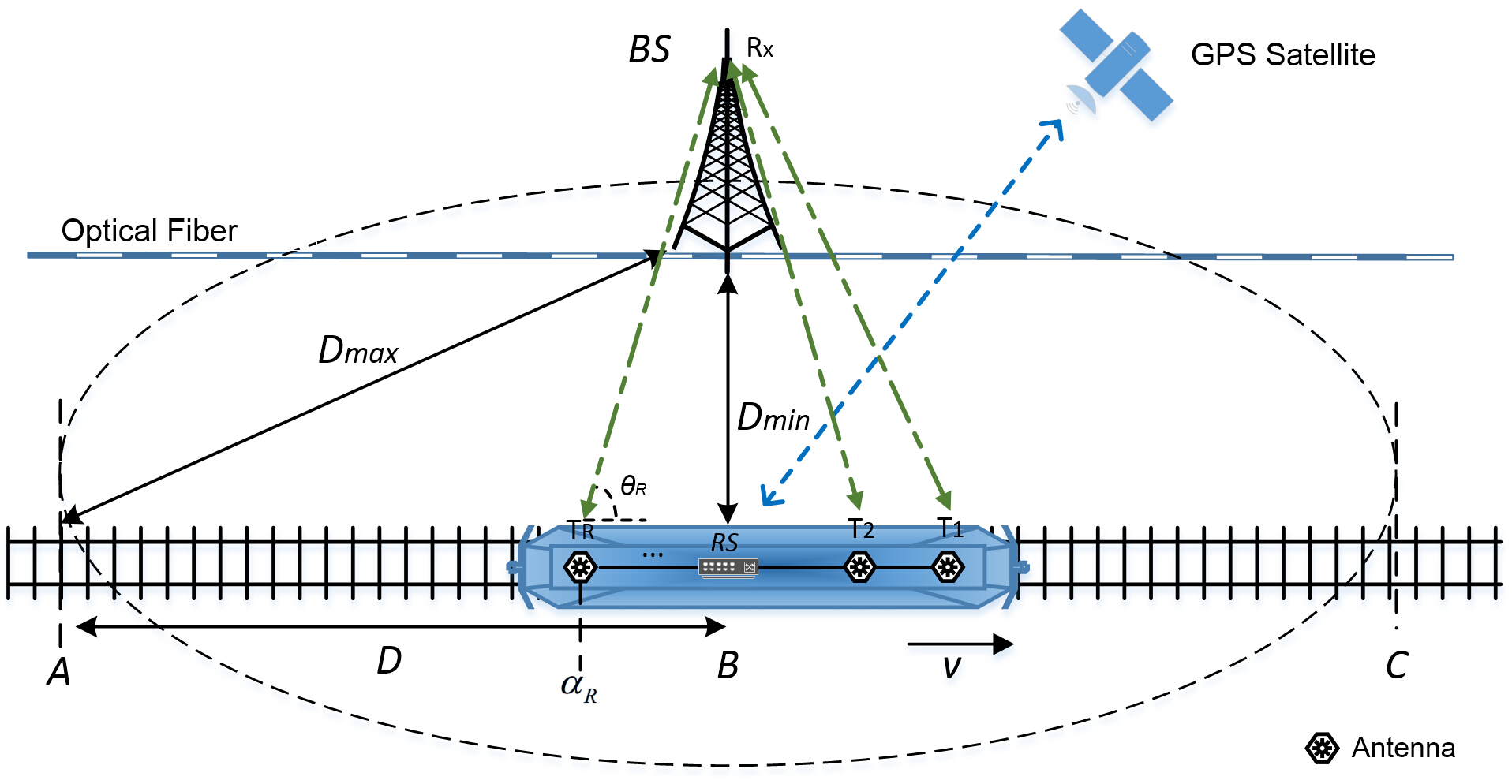
In Fig. 1, we assume that the HST is traveling towards a fixed direction at a constant speed $v$. Let $D_{max}$ denote the maximum distance from the BS to the railway (i.e., the position $A$ and $C$ to $BS$), $D_{min}$ denote the minimum distance (i.e., the position $B$ to $BS$), and $D$ denote the distance between $A$ and $B$. The $R$ receive antennas evenly located on the top of the HST are denoted as $\{T_{r}\}^{R}_{r=1}$, and $R_{x}$ denotes the antenna equipped on the BS. In each cell, we define $\alpha_{r}$ as the distance between the $r$-th receive antenna and the position $A$, and define $\theta_{r}$ as the angle between the BS to $T_{r}$ and the railway. When the HST moves from $A$ to $C$, $\theta_{r}$ changes from $\theta_{min}$ to $\theta_{max}$. If $D_{max}\gg D_{min}$, we have $\theta_{min}\approx 0^{\circ}$ and $\theta_{max}\approx 180^{\circ}$. For $T_{r}$ at a certain position $\alpha_{r}$, it suffers from a Doppler shift $f_{r}$, where $f_{r}$ can be calculated by $f_{r}=\frac{v}{c}\cdot f_{c}\cos\theta_{r}$ with the carrier frequency $f_{c}$ and the the light speed $c$. In addition, we assume that $f_{r}$ is constant within one OFDM symbol.

In this paper, we only consider the first-hop communication in the HST system, i.e., the communication from the BS to the RS. It is treated as a SIMO-OFDM system with one transmit antenna and $R$ receive antennas. Suppose there are $K$ subcarriers. The transmit signal at the $k$-th subcarrier during the $n$-th OFDM symbol is denoted as $X^{n}(k)$, for $n=1,2,...,N$ and $k=1,2,...,K$. At the BS, after passing the inverse discrete Fourier transform (IDFT) and inserting the cyclic prefix (CP), the signals are transmitted to the wireless channel. At the $r$-th receive antenna, after removing the CP and passing the discrete Fourier transform (DFT) operator, the received signals in the frequency domain are represented as

where ${\bf{y}}^{n}_{r}=[Y^{n}_{r}(1),Y^{n}_{r}(2),...,Y^{n}_{r}(K)]^{T}$ is the received signal vector over all subcarriers during the $n$-th OFDM symbol, ${\bf{H}}^{n}_{r}$ is the channel matrix between the transmit antenna and the $r$-th receive antenna, ${\bf{x}}^{n}=[X^{n}(1),X^{n}(2),...,X^{n}(K)]^{T}$ is the transmitted signal vector, and ${\bf{n}}^{n}_{r}=[N^{n}_{r}(1),N^{n}_{r}(2),...,N^{n}_{r}(K)]^{T}$ denotes the noise vector, where $N^{n}_{r}(k)$ is the additive white Gaussian noise (AWGN) with a zero mean and $\sigma^{2}_{\varepsilon}$ variance.

If the channel is time-invariant, the off-diagonal term ${{H}_{r}^{n}({k,d}})$ $(k\neq d)$ in ${\bf{H}}_{r}^{n}$ is negligible, and the diagonal term ${{H}^{n}_{r}({k,d}})$ $(k=d)$ alone represents the channel, where $k,d=1,...,K$. However, for time-varying channel, the off-diagonal term cannot be neglected and (1) can be rewritten as

where ${\bf{H}}_{r_{\rm free}}^{n}\triangleq{\text{diag}}\{[H^{n}_{r}(1,1),H^{n}_{r}(2,2),...,H^{n}_{r}(K,K)]\}$ denotes the ICI-free channel matrix, and ${\bf{H}}_{r_{\rm ICI}}^{n}\triangleq{\bf{H}}^{n}_{r}-{\bf{H}}_{r_{\rm free}}^{n}$ is the ICI part.

In our previous work [21], we adopted the channel model in [8] to model the channel in the delay-Doppler domain. In this work, however, we employ the BEM to model the high-mobility channel in the time domain. Assume that the channel between the transmit antenna and each receive antenna consists of $L$ multi-paths. For each channel tap $l$, $0\leq l\leq L-1$, we define ${\tilde{\bf{h}}}^{n}_{r}(l)=[h^{n}_{r}(0,l),h^{n}_{r}(1,l),...,h^{n}_{r}(K-1,l)]^{T}\in\mathbb{C}^{K\times 1}$ as a vector which collects the time variation of the channel tap within the $n$-th OFDM symbol of the channel between the transmit antenna and the $r$-th receive antenna. Denote $f_{max}$ as the maximum Doppler shift, $T$ as the packet duration, and $Q=2\lceil f_{{max}}T\rceil$ as the maximum number of the BEM order. Then, each $\tilde{\bf{h}}^{n}_{r}(l)$ can be represented as

where ${\bf B}=[{\bf b}_{0},...,{\bf b}_{q},...,{\bf b}_{Q}]\in\mathbb{C}^{K\times(Q+1)}$ collects $Q+1$ basis functions as columns, ${\bf b}_{q}$ denotes the $q$-th basis function ($q=0,1,...,Q$) whose expression is related to a specific BEM model, ${\bf c}^{n}_{r}(l)=[c^{n}_{r}(0,l),c^{n}_{r}(1,l),...,c^{n}_{r}(Q,l)]^{T}$ represents the BEM coefficients for the $l$-th tap of the channel at the $r$-th receive antenna within the $n$-th OFDM symbol, and ${\bm{\epsilon}}^{n}_{r}(l)=[\epsilon^{n}_{r}(0,l),\epsilon^{n}_{r}(1,l),...,\epsilon^{n}_{r}(K-1,l)]^{T}$ represents the BEM modeling error.

Stacking all the channel taps of the $r$-th receive antenna within the $n$-th OFDM symbol in one vector

then we obtain

where ${\bf I}_{L}$ is an $L\times L$ identity matrix, ${\bf c}^{n}_{r}=[c^{n}_{r}(0,0),...,c^{n}_{r}(0,L-1),...,c^{n}_{r}(Q,0),...,c^{n}_{r}(Q,L-1)]^{T}\in\mathbb{C}^{L(Q+1)\times 1}$ is the stacking coefficient vector, and ${\bm{\epsilon}}^{n}_{r}=[\epsilon^{n}_{r}(0,0),...,\epsilon^{n}_{r}(0,L-1),...,\epsilon^{n}_{r}(K-1,0),...,\epsilon^{n}_{r}(K-1,L-1)]^{T}\in\mathbb{C}^{KL\times 1}$. In the following, as our focus is to discuss the performance of the channel estimator and the ICI eliminator, we ignore ${\bm{\epsilon}}^{n}_{r}$ for convenience. We also assume that the coefficients are constant within one OFDM symbol.

Therefore, based on the BEM, we can describe the system in the high-mobility environment. In addition, since we only consider the system in a single OFDM symbol in this paper, the symbol index $n$ is omitted in the sequel for compactness. Then, substituting (5) into (1), we obtain

in which ${\bf D}_{q}={\bf F}{\text{diag}}\{{\bf b}_{q}\}{\bf F}^{H}$ denotes the $q$-th BEM basis function in the frequency domain, ${\bf F}$ is the $K\times K$ DFT matrix, ${\bf\Delta}_{r,q}={\text{diag}}\{{\bf F}_{L}{\bf c}_{r,q}\}$ is a diagonal matrix whose diagonal entries are the frequency responses of ${\bf c}_{r,q}$, ${\bf c}_{r,q}=[c_{r}(q,0),...,c_{r}(q,L-1)]^{T}$ denotes the BEM coefficients of all taps of the $r$-th receive antenna corresponding to the $q$-th basis function, and ${\bf F}_{L}$ denotes the first $L$ columns of $\sqrt{K}{\bf F}$.

We first give a definition of $S$-sparse channels based on the BEM channel model introduced in the previous section.

Then we give the following theorem, which reflects the position information of the given system.

Accordingly, the relationship between the dominant index $q^{*}_{r}$ and $f_{r}$ is given as

Denote ${F}=Tf_{{\max}}=T\frac{v}{c}\cdot f_{c}$. Then the relationship between $q^{*}_{r}$ and $\alpha_{r}$ can be represented as

where ${\alpha_{r}}\in[0,D]$ denotes the $r$-the receive antenna moving from $A$ to $B$, and ${\alpha_{r}}\in(D,2D]$ denotes moving from $B$ to $C$.

From Theorem 1, we readily have the following corollary.

According to Corollary 1, (6) can be simplified as

In this way, we exploit the position information of the BEM and utilize it to simply the required channel coefficients from $L(Q+1)$ to $L$. Note that these analyses and conclusions are not restricted to any specific BEM.

In this subsection, we consider the CE-BEM [26] due to its independence of the channel statistics and it is strictly banded in the frequency domain. Specifically, for the CE-BEM, the $q$-th basis function ${\bf b}_{q}$ can be represented as

Then, the ${\bf D}_{q}$ can be written as

where ${\bf I}^{\langle q-\frac{Q}{2}\rangle}_{K}$ denotes a matrix obtained from a $K\times K$ identity matrix ${\bf I}_{K}$ with a permutation $q-Q/2$. Then, we have

By detecting the matrix structure, we find that ${\bf H}_{r}$ is strictly banded with the bandwidth $Q+1$, which means that the $Q$ neighboring subcarriers give rise to interference, i.e., the desired signal suffers from the ICI from the $Q$ neighboring subcarriers.

Assume that $P~(P<K)$ pilots are inserted in the frequency domain at the BS with the pilot pattern ${\bf w}$, where ${\bf w}=[w_{1},w_{2},...,w_{P}]$. Denote ${\bf d}$ as the subcarrier pattern of the transmitted data. Then, the received pilots at the $r$-th receive antenna is represented as

in which ${\bf D}_{q}({\bf w},{\bf w})$ and ${\bf\Delta}_{r,q}({\bf w},{\bf w})$ represent the submatrices of ${\bf D}_{q}$ and ${\bf\Delta}_{r,q}$ with the row indices ${\bf w}$ and the column indices ${\bf w}$, respectively, ${\bf D}_{q}({\bf w},{\bf d})$ and ${\bf\Delta}_{r,q}({\bf d},{\bf d})$ represent the submatrices with the row indices ${\bf w}$ and $\bf d$ and the column indices ${\bf d}$, respectively, and ${\bf n}_{r}$ is the noise vector at ${\bf w}$. In (15), we decouple the ICI caused by the $Q$ neighboring data from the pilots and put it in the term $\bf G$, which directly degrades the channel estimation accuracy.

Let us consider Corollary 1, then the dominant basis ${\bf D}^{*}_{r}$ for the CE-BEM can be rewritten as

Similarly, we have

where ${\bf H}_{r}$ becomes a diagonal matrix with a permutation and its non-zero entries are corresponding to the dominant coefficients. From (17), we find that, with Corollary 1, the desired signal is free of ICI but with a permutation of the received subcarrier. This is reasonable because the dominant coefficients in ${\bf c}^{*}_{r}$, corresponding to $f_{r}$, describe the channel alone while the non-dominant ones can be ignored. Therefore, by utilizing the position information, we can get the ICI-free pilots at the receive side and also reduce the needed channel coefficients from $KL$ to $L$.

Remark 1: With Corollary 1, the conclusion that ${\bf H}_{r}$ is a permutated diagonal matrix only holds for the CE-BEM, since ${\bf D}_{q}$ itself is a permutated identity matrix for the CE-BEM. For other BEMs, e.g., the GCE-BEM [27], the P-BEM [28], and the DPS-BEM [29], ${\bf D}_{q}$ is approximately banded. However, it can be expected that the proposed method can also highly reduce the ICI for other BEMs for only considering the dominant coefficients.

Assume ${\bf w}$ is received at the $r$-th receive antenna with the pilot pattern ${\bf v}_{r}=[v_{r,1},v_{r,2},...,v_{r,P}]$. Then, with Corollary 1, (15) can be rewritten as

where ${\bf D}^{*}_{r}({\bf v}_{r},{\bf w})$ and ${\bf\Delta}^{*}_{r}({\bf w},{\bf w})$ represent the submatrices with the row indices ${\bf v}_{r}$ and ${\bf p}$ and the column indices ${\bf p}$, respectively, and ${\bf D}^{*}_{r}({\bf v}_{r},{\bf d})$ and ${\bf\Delta}^{*}_{r}({\bf d},{\bf d})$ represent the submatrices with row indices ${\bf v}_{r}$ and ${\bf d}$ and column indices ${\bf d}$, respectively. In (19), the term ${\bf G}^{*}$ denotes the ICI caused by the data, and we have ${\bf G}^{*}={\bf 0}$ since its corresponding entries of the dominant basis are zero, i.e., ${\bf D}^{*}_{r}({\bf v}_{r},{\bf d})={\bf 0}$. Thus, it is easy to find the received pilots are free of the ICI but with a permutation of the received subcarriers. The relationship between ${\bf v}_{r}$ and ${\bf w}$ is given as

where $p=1,2,...,P$, and $|\cdot|_{K}$ denotes the mod $K$ operator.

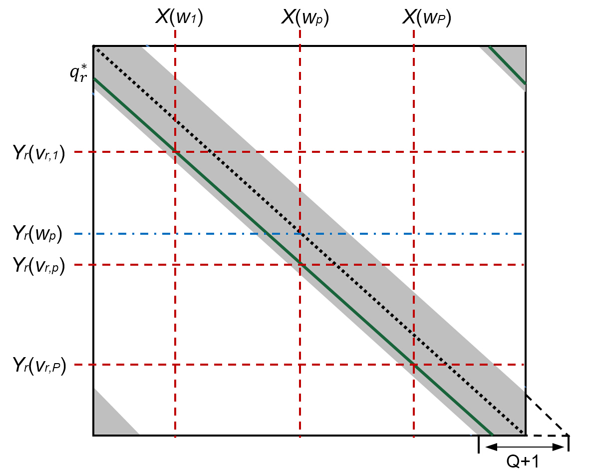
For better clarification, we plot the structure of ${\bf H}_{r}$ in Fig. 2. The columns of ${\bf H}_{r}$ are related to the subcarriers of the transmitted pilots and data, which operate on ${\bf D}_{q}$ through ${\bf\Delta}_{r,q}$. The rows of ${\bf H}_{r}$ are related to the subcarriers of the received signals at the $r$-th receive antenna. For the CE-BEM, ${\bf H}_{r}$ is strictly banded with the bandwidth $Q+1$, which is shown as the grey parts. From Fig. 2, it can be observed that a received signal $Y_{r}(w_{p})$ suffers from the ICI from the $Q$ neighbouring subcarriers of its desired signal $X(w_{p})$, which is shown as the blue dash dot line. Then, with Corollary 1, ${\bf H}_{r}$ turns to the green solid line and the grey parts can be neglected, which is because the dominant coefficients alone describe the channel with the Doppler shift $f_{r}$. It is easy to find that the desired signal $X(w_{p})$ is free of the ICI but received at $Y(v_{r,p})$ with a permutation of the received subcarrier, which is shown as the red dash lines. Therefore, with the proposed method, the ICI among the received pilots at each receive antenna is eliminated.

CS is an innovative technique to reconstruct sparse signals accurately from a limited number of measurements. Considering an unknown signal ${\hat{\bf{x}}}\in\mathbb{C}^{M}$, suppose that we have ${\hat{\bf{x}}}=\bf{\Phi}\bf{a}$, where ${\bf{\Phi}}\in{\mathbb{C}}^{M\times U}$ denotes a known dictionary matrix and ${\bf a}\in{\mathbb{C}}^{U}$ denotes a $S$-sparse vector, i.e., $\|{\bf{a}}\|_{{{{\ell}_{0}}}}=S\ll U$. Then, CS considers the following problem

in which ${\bf{\Psi}}\in{\mathbb{C}}^{V\times M}$ presents a known measurement matrix, ${\hat{\bf y}}\in{\mathbb{C}}^{V}$ presents the observed vector, and ${\bm{\eta}}\in{\mathbb{C}}^{V}$ is the noise vector. The objective of CS is to reconstruct $\bf{a}$ accurately based on the knowledge of ${\hat{\bf y}}$, $\bf\Psi$, and $\bf{\Phi}$. It has been proved in [13] that if $\bf{\Psi\Phi}$ satisfies the restricted isometry property (RIP) [30], then $\bf a$ can be reconstructed accurately with CS reconstruction methods, such as the basis pursuit (BP) [31] and the orthogonal matching pursuit (OMP) [32]. In addition, a fundamental research [14] indicates that the average coherence reflects the actual CS behavior rather than the mutual coherence [12] for considering the average performance. The definition of the average coherence is given as follows.

It has been established in [14] that a smaller $\mu_{\delta}\{\bf{\Psi\Phi}\}$ will lead to a more accurate recovery of $\bf a$. From this point of view, it can be expected that if $\bf{\Psi}$ is designed with a fixed $\bf{\Phi}$ such that ${{\mu_{\delta}}\left\{{\bf{\Psi\Phi}}\right\}}$ is as small as possible, then CS can get better recovery performance.

To utilize the sparsity of the high-mobility channel according to Theorem 1, we rewrite the received pilots at the $r$-th antenna as a function of channel coefficients. In this paper, we assume that each receive antenna estimates its channel individually, and then sends the estimated channel to the RS for operation. Then, (19) can be rewritten as

where ${\bf S}({\bf w},:)={\text{diag}}\{{\bf x}({\bf w})\}{\bf F}_{L}({\bf w},:)$. In this way, the task of estimating the high-mobility channel ${\bf H}_{r}$ in the frequency domain is converted to estimating the sparse coefficient vector ${\bf c}_{r}^{*}$.

As aforementioned in the pervious subsection, we have known that a lower $\mu_{\delta}$ leads to a better CS performance. Therefore, we propose to design the pilot pattern ${\bf w}$ to minimize the average coherence in our system. In this paper, we only design the pilot pattern and assume the pilot symbols are the same. Therefore, the global pilot pattern design problem can be formulated as

where ${\bf w}^{*}$ denotes the optimal pilot pattern, and $r=1,2,...,R$. Note that for a given ${\bf w}$, its corresponding ${\bf v}_{r}$ at the $r$-th receive antenna can be obtained by (20). Thus, ${\bf w}$ is the only variable in this problem.

Taking the expression of ${\bf D}^{*}_{r}$ into consideration, the objective function can be represented as

where we have ${\bf I}^{\langle{q^{*}_{r}}-\frac{Q}{2}\rangle}_{K}({\bf v}_{r},{\bf w})={\bf I}_{P}$ for $r=1,2,...,R$, and ${\bf I}_{P}$ denotes a $P\times P$ identity matrix. This is because ${\bf v}_{r}$ and ${\bf w}$ are designed by the given equation (20) to select the non-zero entries of ${\bf D}^{*}_{r}$.

Suppose that each pilot symbol has the same constant amplitude, i.e.,

According to Definition 2, it is not difficult to prove that the average coherence is independent of the constant amplitude. Thus, the objective function can be further written as

In this way, the problem (25) is simplified to the following optimization problem

From (31), we find that the optimal pilot pattern ${\bf w}^{*}$ is independent of the train speed $v$, the Doppler shift $f_{r}$, the antenna number $R$, or the antenna position $\alpha_{r}$. This means that ${\bf w}^{*}$ is global optimal, regardless of the receive antenna number, the antenna position, the Doppler shift, or the train speed. Thus, for the given system, we can pre-design ${\bf w}^{*}$ and then sends it to each receive antenna to estimate the channel during the whole system runs. Note that the problem (31) is different from the problem in our previous work [21], where the optimal pilot was related to the Doppler shift according to the instant train position.

The similar pilot design problems for SISO-OFDM systems have been studied in [22] and our previous work [21]. However, these methods cannot be directly applied to (31). The problem in [22] includes the guard pilots and needs to follow some constraints to eliminate the ICI. In addition, the optimal pilot in [21] is related to the instant train position. In this subsection, following the spirit of [21], we propose a low complexity suboptimal pilot pattern design algorithm to solve this problem. The details are presented in Algorithm 1.

In Algorithm 1, ${\bf{w}}^{(m)}$, $\tilde{\bf{w}}^{(m)}$, and $\hat{\bf{w}}^{(m)}$ are defined as different pilot pattern sets at the $m$-th iteration. $M$ is the number of pilot pattern sets, and $Iter=M\times P$ denotes the total iteration times. The probability vector ${\bf{\Gamma}}[m]=[\Gamma[m,1],\Gamma[m,2],...,\Gamma[m,MP]]^{T}$ represents the state occupation probabilities with entries ${{\Gamma}}[m,\kappa]\in[0,1]$, and $\sum_{\kappa}{{\Gamma}}[m,\kappa]=1$. ${\bf{U}}[m]\in\mathbb{R}^{MP\times 1}$ is defined as a zero vector except for its $m$-th entry to be 1. In Step a), $\tilde{\bf{w}}^{(m)}$ is obtained with the operator ${\bf{w}}^{(m)}\Rightarrow\tilde{\bf{w}}^{(m)}$, which is defined as: at the $m$-th iteration, the $k$-th pilot subcarrier of ${\bf{w}}^{(m)}$ is replaced with a random subcarrier which is not included in ${\bf{w}}^{(m)}$. Then, we compare ${{\tilde{\bf{w}}}^{(m)}}$ with ${{{\bf{w}}}^{(m)}}$ and select the one with a smaller system coherence to move a step. In Step b), ${\bf{\Gamma}}[m+1]$ is updated based on the previous ${\bf{\Gamma}}[m]$ with the decreasing step size $\eta[m]=1/(m+1)$. The current optimal pattern is updated by selecting the pilot pattern with the largest occupation probability. Finally, the optimal pilot pattern is obtained as ${\bf w}^{*}=\hat{\bf w}^{(MP)}$. According to [21], this process can quickly converge to the optimal solution.

Remark 2: In contrast to the work in [22], Algorithm 1 does not need any guard pilot to eliminate the ICI, which highly improves the spectral efficiency. This is because the received pilots are ICI-free at each receive antenna with the proposed ICI elimination method. In specific, the total needed pilot number in [22] is $(2Q+1)P$ ($P$ effective pilots and $2QP$ guard pilots), while our method only needs $P$ pilots.

Here we briefly discuss the complexity of our proposed scheme. The complexity is mainly determined by the number of the needed complex multiplications. The complexity of the proposed scheme mainly consists of two parts: the low coherence pilot pattern design (Algorithm 1) and the position-based ICI elimination.

• •

  For Algorithm 1, it requires $MP^{2}(L(L-1)+M)$ complex multiplications in total. In a practical system, as the constant parameters $M$, $L$, and $P$ are much smaller than $K$, the complexity of Algorithm 1 is much lower than ${\mathcal{O}}(K^{2})$. Furthermore, since the needed system parameters can be estimated in advance, Algorithm 1 is an off-line process and thus its complexity can be omitted in practice.

• •

  For our ICI elimination method, with known the optimal pilot pattern pre-designed by Algorithm 1, the $r$-th antenna obtains its receive pilot pattern by (20) at any given position. This process only needs a permutation of the subcarriers, where the needed $q^{*}_{r}$ can be directly calculated from the HST’s current speed and position information supported by the GPS. Thus, the proposed ICI elimination method introduces very low complexity in practical systems.

In addition, we also compare the system complexity of the proposed scheme and the scheme in our previous work [21] in SIMO systems. Note that the scheme in [21] cannot directly extend to the SIMO system. For SIMO systems, since the length of the HST cannot be ignored comparing with the cell range in practice, the receive antennas may suffer from different Doppler shifts and correspond to different optimal pilots. To solve this problem, based on the scheme in [21], one may divide the total $P$ pilots into $R$ subsets, and each subset sends the corresponding optimal pilot for each receive antenna to minimize the system coherence. In the presence of large number of the receive antennas (i.e., large $R$), this method will introduce high system complexity for selecting different optimal pilots. In addition, since the effective pilot number for each receive antenna is $P/R$, a large $R$ will also highly reduce the spectral efficiency for needing more total pilots to get satisfactory estimation performance. However, for the proposed method in this work, since ${\bf w}^{*}$ is independent of the receive antenna position and receive antenna number, with increasing $R$, each receive antenna can still have $P$ effective pilots.

Now we briefly discuss the applicability of the proposed scheme in a practical HST system. The entire process of our proposed scheme is summarized as follows:

1. 1.

   For a given HST system, as the system parameters can be collected in advance, the optimal pilot pattern ${\bf w}^{*}$ is pre-designed by Algorithm 1 and then pre-stored at both the BS and the HST. Since ${\bf w}^{*}$ is independent of the Doppler shift or the train position, the BS transmits ${\bf w}^{*}$ to estimate the channels during the whole process. In contrast, in our previous work [21], the BS was required to select different optimal pilot for each receive antenna from a pre-designed codebook according to the instant train position, which introduces high system complexity.

2. 2.

   Then, the antennas on the HST receive the signals and get the ICI-free pilots with the proposed ICI elimination method, which is given as (20). In addition, with the instant train position and speed information supported by the GPS, ${q^{*}_{r}}$ of each receive antenna can be easily calculated with the given equations (8) and (9).

3. 3.

   After that, each receive antenna uses the ICI-free pilots to estimate the channel coefficients with the conventional CS estimators.

In this way, the proposed scheme can be well used in current HST systems without adding too much complexity. Note that, as ${\bf w}^{*}$ is also independent of the train speed, the performance of the proposed scheme is robust to the high mobility. This is interesting because that the channel estimation performances are always highly influenced by the high system mobility [21][23]. In the following section, we will give some simulation results to demonstrate the effectiveness of the proposed algorithm.

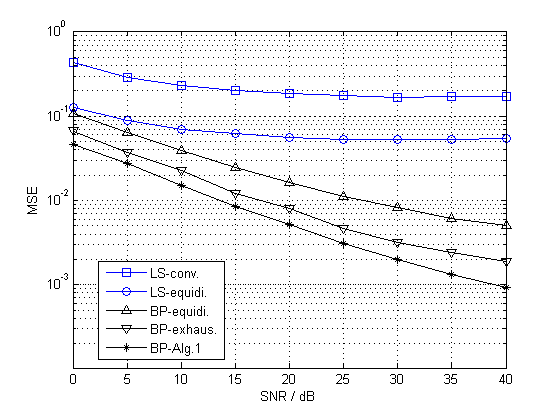
Fig. 3 gives the comparison of the MSE performances of different estimators with different pilot patterns at the position $A$, where the Doppler shift at the receive antenna is $1.087$KHz. In this figure, we compare three pilot pattern design methods. The equidistant method (“equidi.”) is the equidistant pilot pattern in [5], which is claimed in [5] as the optimal pilot pattern to doubly selective channels. The exhaustive method (“exhaus.”) is the method in [15] with $200$ iterations, which does an exhaustive search from a designed pilot pattern set. The iteration time of Algorithm 1 is set to be $Iter=200$, which is shown in [21] that $Iter=200$ is good enough for a practical system. The “LS-equidi.” method, the “BP-equidi.” method, the “BP-exhaus.” method, and the “BP-Alg.1” method are equipped with the proposed ICI elimination method. In addition, the conventional LS method with the equidistant pilot pattern (“LS-conv.”) is equipped with the ICI mitigation method in [23] with 2 iteration times. It can be observed that the BP estimators significantly improve the performances than the LS methods by utilizing the sparsity of the high-mobility channels. Furthermore, it is found that the estimators with the proposed ICI elimination method get better performances than the one with the conventional method, which means that the proposed method effectively eliminates the ICI. As expected, comparing with other pilot patterns, Algorithm 1 improves the MSE performance for effectively reducing the system average coherence.

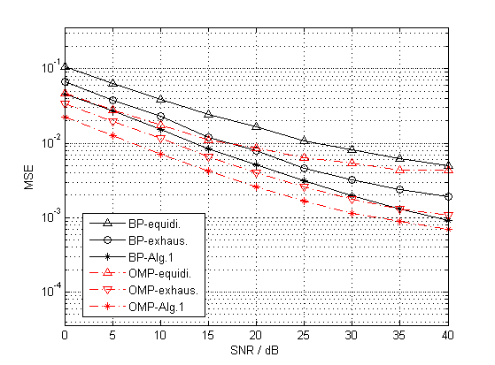
Fig. 4 depicts the comparison of the MSE performances of BP and OMP estimators versus SNR with different pilot patterns at the position $C$, where the Doppler shift at the receive antenna is $-1.087$KHz. All of BP and OMP estimators are considered with the proposed ICI elimination method. As can be seen, with Algorithm 1, both BP and OMP get better performances comparing with other pilot patterns. It can be seen that the proposed algorithm is effective to both BP and OMP estimators.

Fig. 5 presents the MSE performances of BP estimators versus SNR with the proposed ICI elimination method and the conventional ICI mitigation method, where the Doppler shift at the receive antenna is $f_{r}=1.009$KHz according to $\alpha_{r}=900$m. The ICI mitigation is considered with the iteration time as 0, 1, 3, and 5 to show the performance tendency. All of these estimators are equipped with the pilot pattern designed by Algorithm 1 ($Iter=200$). It can be observed that, with increasing iterations, the BP with the ICI mitigation method converges to the one with the proposed ICI elimination method, which gets the ICI-free pilots as aforementioned analysis. In addition, we also notice that the ICI mitigation gain is limited with increasing iteration times due to the error propagation.

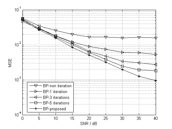
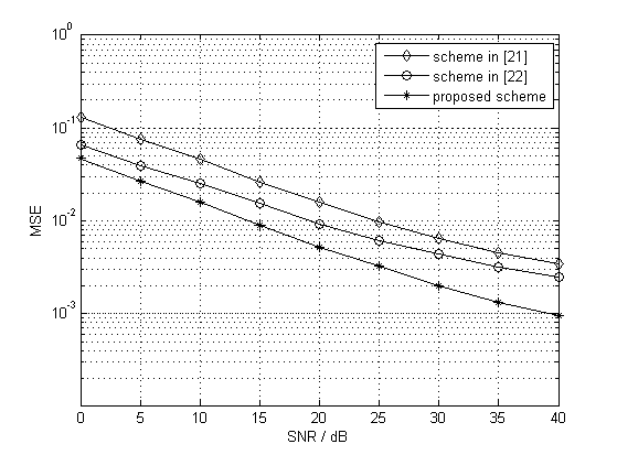
Fig. 6 compares the MSE performances versus SNR of the proposed scheme, the scheme in [21], and the scheme in [22], where the Doppler shift at the receive antenna is $f_{r}=1.087$KHz. The proposed scheme and the scheme in [21] are both considered with 40 pilots and equipped with the proposed ICI elimination method. However, since the optimal pilot in [21] is related to the instant antenna position, we divide the 40 pilots into two sets to send the optimal pilots for each antenna (20 effective pilots for each one). In addition, the scheme in [22] is considered with the guard pilots to get the ICI-free structure, and its total pilot number is $243$. Note that it needs $216$ guard pilots to eliminate the ICI, and thus its effective pilot number is $27$. In this figure, it can be observed that the proposed scheme gets better performance with the same pilot number as [21]. It is mainly because the optimal pilot for the proposed scheme is independent of the instant antenna position, i.e., the $R$ receive antennas correspond to the same optimal pilot, thus, each receive antenna has 40 effective pilots. Furthermore, we notice that the proposed scheme is better than the scheme in [22] with less pilot number. This is because the proposed ICI elimination method only needs a permutation of the receive subcarriers without needing any guard pilot, which highly improves the spectral efficiency.

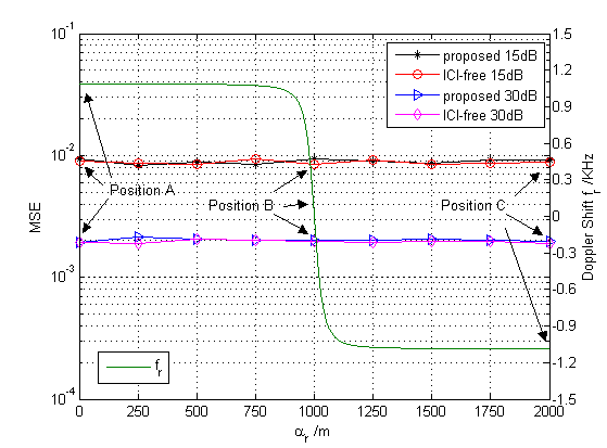
Fig. 7 presents the MSE performances of BP estimators versus the receive antenna position at SNR = $15$dB and SNR = $30$dB. As a reference, we also plot the Doppler shift $f_{r}$ at the $r$-th receive antenna versus its position $\alpha_{r}\in[0,2000]$m (from $A$ to $C$). We can find that $f_{r}$ changes from $f_{max}$ to $-f_{max}$ with the HST moves, and it changes rapidly near the position $B$. In this figure, the resulting curves correspond to the performances when the proposed ICI elimination method is performed and when the estimation considers that pilots are free of ICI (“ICI-free”) at SNR= 15dB and 30dB, respectively. When the pilots are free of ICI, it means that the transmitted OFDM symbol is set as zero at the data subcarriers. All estimators are considered with the pilot pattern designed by Algorithm 1 ($Iter=200$). From the curves, it can be observed that the proposed method and the ICI-free method are almost superimposed, which means that the proposed method can effectively obtain the ICI-free pilots. In addition, we also notice that, although the HST suffers from large Doppler shift at most of the positions and $f_{r}$ changes rapidly near $B$, the MSE performances of the proposed method are stable. This is because the optimal pilot pattern and the proposed ICI elimination method are both independent of the position information and the system mobility. Thus, the proposed scheme is robust with respect to high mobility.

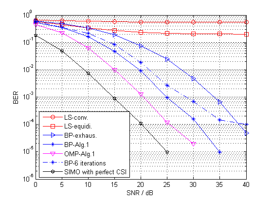
Fig. 8 shows the BER performances versus SNR of the $1\times 2$ SIMO-OFDM system in the given high-mobility environment at the position $A$, where the Doppler shifts at the receive antennas are both $1.087$KHz. In this figure, we compare the LS, the BP, and the OMP estimators with the pilot patterns designed by the equidistant method, the exhaustive method, and Algorithm 1 ($Iter=200$). The conventional LS method (“LS-conv.”) is considered with the one-tap equalization, and other methods are considered with the zero-forcing (ZF) equalizer. As a reference, we also plot the performance with the perfect knowledge of channel state information (CSI), which means that the CSI is available at the RS and employed with the ZF equalizer. In addition, the BP estimator with Alg. 1 and the ICI mitigation method of 6 iteration times is also considered. As can be seen, BP and OMP with Algorithm 1 are closer to the perfect knowledge of CSI. It is also shown that “BP-Alg.1” with the proposed ICI elimination method outperforms the one with the conventional ICI mitigation method for effectively eliminating the ICI. In addition, it can be observed that the pilot pattern designed by Algorithm 1 significantly improves the performances for effectively reducing the system coherence.

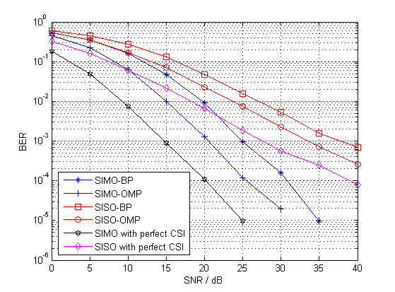
Fig. 9 compares the BER performances between the $1\times 2$ SIMO-OFDM system and the SISO-OFDM system in the given high-mobility environment at the position $A$. Both of the SIMO and the SISO systems are considered with $40$ pilots. All estimators are equipped with the pilot pattern designed by Algorithm 1 and the proposed ICI elimination method. As a reference, we plot the performances with the perfect knowledge of CSI for both the SIMO and SISO systems. It can be observed that the SIMO system significantly improves the BER performances due to the spatial diversity introduced by multiple antennas.

References

- [1] Y. Mostofi and D. C. Cox, “ICI mitigation for pilot-aided OFDM mobile systems,” IEEE Trans. Wireless Commun., vol. 4, no. 2, pp. 765-774, March 2005.
- [2] K. Kwak, S. Lee, H. Min, S. Choi, and D. Hong, “New ofdm channel estimation with dual-ICI cancellation in highly mobile channel,” IEEE Transactions on Wireless Communications, vol. 9, no. 10, pp. 3155-3165, Oct. 2010.
- [3] Z. Tang, R. C. Cannizzaro, G. Leus, and P. Banelli, “Pilot-assisted time-varying channel estimation for OFDM systems,” IEEE Transactions on Signal Processing, vol. 55, no. 5, pp. 2226-2238, May 2007.
- [4] H. Hijazi and L. Ros, “Polynomial estimation of time-varying multipath gains with intercarrier interference mitigation in OFDM systems,” IEEE Transactions on Vehicular Technology, vol. 58, no. 1, pp. 140-151, Jan. 2009.
- [5] X. Ma, G. Giannakis, and S. Ohno, “Optimal training for block transmissions over doubly-selective wireless fading channels,” IEEE Trans. Signal Process, vol. 51, no. 5, pp. 1351-1366, May 2003.
- [6] W. U. Bajwa, A. M. Sayeed, and R. Nowak. “Sparse multipath channels: modeling and estimation,” IEEE Digital Signal Processing Education Workshop, pp. 320-325, Jan. 2009.
- [7] W. U. Bajwa, J. Haupt, A. M. Sayeed, and R. Nowak, “Compressed channel sensing: a new approach to estimating sparse multipath channels,” Proceedings of the IEEE, vol. 98, no. 6, pp. 1058-1076, June 2010.
- [8] W. U. Bajwa, A. M. Sayeed, and R. Nowak, “Learning sparse doubly-selective channels,” 46th Annual Allerton Conference on Communication, Control and Computing, pp. 575-582, Sept. 2008.
- [9] G. Taubock and F. Hlawatsch, “A compressed sensing technique for OFDM channel estimation in mobile environments: exploiting channel sparsity for reducing pilots,” IEEE International Conference on Acoustics, Speech and Signal Processing (ICASSP), pp. 2885-2888, March 2008.
- [10] G. Taubock, F. Hlawatsch, D. Eiwen, and H. Rauhut, “Compressive estimation of doubly selective channels in multicarrier systems: leakage effects and sparsity-enhancing processing,” IEEE Journal of Selected Topics in Signal Processing, vol. 4, no. 2, pp. 255-271, April 2010.
- [11] C. Berger, Z. Wang, J. Huang, and S. Zhou, “Application of compressive sensing to sparse channel estimation,” IEEE Commun. Mag., vol. 48, no. 11, pp. 164-174, Nov. 2010.
- [12] D. L. Donoho, M. Elad, and V. N. Temlyakov, “Stable recovery of sparse overcomplete representations in the presence of noise,” IEEE Trans. Inf. Theory, vol. 52, no. 1, pp. 6-18, Jan. 2006.
- [13] E. J. Candes, J. Romberg, and T. Tao, “Robust uncertainty principles: exact signal reconstruction from highly incomplete frequency information, IEEE Trans. Inf. Theory, vol. 52, no. 2, pp. 489-509, Feb. 2006.
- [14] M. Elad, “Optimized projections for compressed sensing,” IEEE Transcation on Signal Processing, vol. 55, no. 12, pp. 5695-5702, Dec. 2007.
- [15] X. He and R. Song, “Pilot pattern optimization for compressed sensing based sparse channel estimation in OFDM systems,” International Conference on Wireless Communications and Signal Processing (WCSP), pp. 1-5, Oct. 2010.
- [16] N. Jing, W. Bi, and L. Wang, “Deterministic pilot design for MIMO OFDM system based on compressed sensing,” International Conference on Communication Technology (ICCT), pp. 897-903, Nov. 2012.
- [17] D. Wang and X. Hou, “Compressed MIMO chanel estimation and efficient pilot pattern over Doppler sparse environment,” International Conference on Wireless Communications and Signal Processing (WCSP), pp. 1-5, Nov. 2011.
- [18] C. Qi and L. Wu, “Optimized pilot placement for sparse channel estimation in OFDM systems,” IEEE Signal Processing Letters, vol. 18, no. 12, pp. 749-752, Dec. 2011.
- [19] C. Qi and L. Wu, “A study of deterministic pilot allocation for sparse channel estimation in OFDM systems,” IEEE Communications Letters, vol. 16, no. 5, pp. 742-744, May 2012.
- [20] X. Ren, W. Chen, and Z. Wang, “Low coherence compressed channel estimation for high mobility MIMO OFDM systems,” Global Communications Conference (GLOBECOM), Dec. 2013.
- [21] X. Ren, W. Chen, and M. Tao, “Position-based compressed channel estimation and pilot design for high-mobility OFDM systems,” IEEE Transactions on Vehicular Technology, July 2014. (Accepted)
- [22] P. Cheng, Z. Chen, Y. Rui, Y. Guo, L. Gui, M. Tao, and Q. T. Zhang “Channel estimation for OFDM systems over doubly selective channels: a distributed compressive sensing based approach,” IEEE Transaction on Communications, vol. 61, no. 10, pp. 4173-4185, Oct. 2013.
- [23] H. Hijazi and L. Ros, “Joint data QR-detection and kalman estimation for OFDM time-varying rayleigh channel complex gains,” IEEE Trans. Commun., vol. 58, no. 1, pp. 170-178, 2010.
- [24] L. Liu, C. Tao, J. Qiu, H. Chen, L. Yu, W. Dong, and Y. Yuan, “Position-based modeling for wireless channel on high-speed railway under a viaduct at 2.35 GHz,” IEEE Journal on Selected Areas in Communications, vol. 30, no. 4, pp. 834-845, May 2012.
- [25] R. D. Pascoe and T. N. Eichorn, “What is communication-based train control?,” IEEE Vehicular Technology Magazine, vol. 4, no. 4, pp. 16-21, Dec. 2009.
- [26] A. P. Kannu and P. Schniter, “MSE-optimal training for linear time-varying channels,” Proc. IEEE Int. Conf. Acoust., Speech, Singal Process. (ICASSP), pp. 789-792, Mar. 2005.
- [27] G. Leus, “On the estimation of rapidly time-varying channels,” Euro. Signal Process. Conf. (EUSIPCO), Sep. 2004.
- [28] D. K. Borah and B. D. Hart, “Frequency-selective fading channel estimation with a polynomial time-varying channel model,” IEEE Trans. Commun., vol. 47, no. 6, pp. 862-873, Jun. 1999.
- [29] T. Zemen and C. F. Mecklenbräuker, “Time-variant channel estimation using discrete prolate spheroidal sequences,” IEEE Trans. Signal Process., vol. 53, no. 9, pp. 3597-3607, Sep. 2005.
- [30] E. J. Candes and M. B. Wakin, “An introduction to compressive sampling,” IEEE Signal Processing Mag., vol. 25, no. 2, pp. 21-30, March 2008.
- [31] S. S. Chen, D. L. Donoho, and M. A. Saunders, “Atomic decompostiion by basis pursuit,” SIAM Review, vol. 43, pp. 129-159, 2001.
- [32] Y. C. Pati, R. Rezaiifar, and P. S. Krishnaprasad, “Orthogonal matching pursuit: recursive function approximation with applications to wavelet decomposition,” Proceedings of the 27th Annual Asilomar Conference on Signals, Systems and Computers, vol. 1, pp. 40-44, Nov. 1993.