remarkRemark \newsiamremarkhypothesisHypothesis \newsiamthmclaimClaim \headers-capacity of general setsJ. P. Nolan, D. J. Audus, and J. F. Douglas
Computation of Riesz -capacity of general sets in using stable random walks††thanks: Submitted to the editors August 19, 2025.
Abstract
A method for computing the Riesz -capacity, , of a general set is given. The method is based on simulations of isotropic -stable motion paths in -dimensions. The familiar Walk-On-Spheres method, often utilized for simulating Brownian motion, is modified to a novel Walk-In-Out-Balls method adapted for modeling the stable path process on the exterior of regions “probed” by this type of generalized random walk. It accounts for the propensity of this class of random walk to jump through boundaries because of the path discontinuity. This method allows for the computationally efficient simulation of hitting locations of stable paths launched from the exterior of probed sets. Reliable methods of computing capacity from these locations are given, along with non-standard confidence intervals. Illustrative calculations are performed for representative types of sets K, where both and are varied.
keywords:
Keywords: generalized capacity, stable processes, potential theory, U-statisticsMathematics Subject Classifications: 31B02, 31B15, 31A15, 31C02, 60G52
1 Introduction
The capacity of a set is a measure of the “size” of the set, and when combined with the volume of the set, this quantity gives information about the shape of the set. Capacity is related to many physical properties of an object, e.g. the electrostatic capacity of charged objects, the influence of the shape of reactive particles on the rate of diffusion-limited chemical reactions, how objects diffuse in liquids, how heat flows to and from an object, etc. These and other applications are discussed in Douglas et al. [9]. Recent work has shown that the shape of a biological cell is relevant to its functions, and Betancourt et al. [1] use capacity as a metric for quantifying cell shapes.
Recently, there has been great interest in “generalized boundary value problems” involving “fractional diffusion processes” related to Lévy stable processes. The connection between these fractional differential equations and Lévy stable path processes arises from the fact that the fractional Laplacian is the generating operator of Lévy stable processes. There has also been interest and scientific activity in numerical computations aimed at obtaining solutions of this type of generalized boundary value problem based on formal extensions of classical probabilistic potential theory ideas developed for Brownian motion, whose generator is the ordinary Laplacian operator, to solving fractional differential boundary value problems. There are many unsolved problems in this active field of study, and we mention the related numerical study of Kyprianou et al. [19], which addresses the solution of extensions of classical interior boundary value problems, such as Poisson equation, where the sampling of the well-known walk-on-sphere (WOS) methodology was utilized as in previous numerical simulations based on ordinary random walks. Encouragingly, they found that it was possible to obtain numerical results in good agreement with the limited known analytic results for stable processes. In contrast, our paper is devoted to an extension of the solution of Laplace’s equation on the exterior of a generally shaped region in dimensions, the exterior Dirichlet problem. We are in particular interested in precisely estimating the Riesz alpha capacity in spatial dimensions, which describes how the harmonic solution to this classical exterior boundary value problem decays at large distances from . We find that the treatment of this type of exterior problem unfortunately does not admit to the simple WOS methodology because of the non-continuity of the Lévy path processes for so that we must introduce new methods of accelerating the path sampling required for our exterior boundary value problem simulations of .
The capacity is a shape functional that has numerous applications. Methodologies attempting to estimate this fundamental quantity are discussed at length in the classic work by Polyá and Szegö [29]. It is well known that the accurate numerical estimation of capacity is quite difficult to achieve, except few exceptional sets, and that even numerical estimation based on finite element and other methods can be very challenging. In recent years, however, a powerful and fast algorithm has been developed that allows for the calculation of ordinary capacity (when ) to unprecedented accuracy. The aim here is to develop an extension of the current algorithm to describe for the purpose of providing a computational tool for addressing diverse shape discrimination problems. We emphasize that the method of solution developed by [19] should be valuable in solving for functionals of associated with interior boundary value problems such the “torsional rigidity” and the related problem of calculating velocity field in pipes having a general cross-sectional shape as in Hunt et al. [13]. The methods are thus complementary.
We term our methodology for accelerating the path averaging process for the exterior Dirichlet problem the Walk-In-Out-of-Balls (WIOB) method. The name of this method derives taking the starting distribution of launch sites for our paths to be located within a spherical ball rather from the boundary of such a ball as in the former WOS computations of 2-capacity in the case of Brownian paths. This distribution of launch sites in our path averaging simulations derives from the equilibrium charge density of the stable process hitting a solid sphere when launched from the exterior of the ball. For Brownian paths, the launch points are localized to the sphere surface because the charge density is localized to the spherical surface, a fact that greatly simplifies the calculation in this case. This is why the simple walk-on-sphere method can be readily applied in the Brownian motion for the exterior problem when the launch sphere concept is utilized to embed the set . We further emphasize that the exterior problem has other features that make it rather distinct from its interior analog. Capacity is fundamentally related to probability of the path process to escape to infinity, and thus depends strongly on the spatial dimensionality in addition to the “shape” and “size” of . Paths initiating from the interior of (compact) never escape to infinity so that the transience of the generalized random walk process (existence of a positive probablity of ultimate escape to infinity) is not a consideration in interior calculations. In contrast, capacity is only a positive finite quantity when the escape probability is finite and positive and this limits the values of and for which can be meaningfully defined.
The novelty of our approach is not limited to the development of the WIOB method, which might be useful in other fractional diffusion exterior boundary value problems. The numerical calculations of the energy integral involve U-statistics. However, standard U-statistic theory does not work here because the summands are heavy tailed with infinite variance. Using standard -statistics theory sometimes gives unreliable estimates of the energy integral. Indeed, it sometimes gives estimates of variance that are negative. We also want to be able to detect when the energy integral is infinite, but the finite sum approximation in section 3.2 to equation (1) is always finite. We provide a novel approach for solving these numerical problems that we expect to have general utility in the solution of exterior fractional boundary value problems. As another point related to the novelty of the present work, we consider a range of representative numerical computations in dimensions: and 5. We are not aware of any numerical estimations of even ordinary capacity in any dimension other than or . We also explore -capacity when for hollow objects. Ordinary capacity cannot probe the interior of hollow sets; -capacity can. We also discuss how -capacity can be used to estimate the fractal (Hausdorff) dimension of sets and illustrate this type of calculation in the simple case of a disc shaped region embedded in . We expect that the capacity to probe information in the interior of sets and to estimate fractal dimension and other geometrical properties of sets should be useful in numerous future practical applications regarding shape discrimination and quantification.
We review the analytic definition of capacity given by Riesz [34]. For and a Borel probability measure on , the energy integral is defined by,
| (1) |
The kernel of this energy functional derives from the potential associated with Lévy random walks. For a compact Borel set , the -capacity or Riesz -capacity of is defined by the functional:
where the infimum is over all probability measures with support. Landkof [20] shows that there is a unique probability measure that minimizes the energy integral, which is called the -equilibrium measure of .
The classical capacity corresponds to the case in which , and has been variously termed the electrostatic capacity or Coulombic capacity or the Newtonian capacity. We note that the case , defined above is finite and it is not equal the logarithmic capacity. We will not discuss the logarithmic capacity in the present work, see Riesz [34] or Landkof [20] for that case. Also, some authors introduce a multiplicative constant in (1), which can lead to confusion about the values of capacity. In the present work, the definition of 2-capacity follows the scaling used in Riesz [34] and in the ZENO program of Mansfield and Douglas [21] and Juba et al. [15]. In particular, the 2-capacity of a ball of radius in is for any . We note that unfortunately there is another mathematical quantity that is designated “-capacity” in the mathematical literature, see Kruglikov [18], motivating the more specific terminology “Riesz -capacity” used here.
Only a few sets have known capacity even when and . These cases are listed on pages 146-147 of Schiffer and Szego [37] and pages 165-167 of Landkof [20]. Polya and Szego [29] assert that it is unlikely that there will ever be an analytic method of computing capacity for more general sets. The work of Mansfield et al. [22] and Mansfield and Douglas [21] developed probabilistic methods based on the paths of Brownian motion for estimating the 2-capacity of complex shapes in three dimensions to understand some of their physical properties. The resulting algorithm, called ZENO, is based on simulating Brownian motion paths. The program enables precise calculation of the 2-capacity for complicated objects in dimension , e.g. polymers and proteins composed of a large number of atoms. This general topic is discussed in Vargas-Lara et al. [44]. (The program is called ZENO in honor of the famous paradox of Zeno regarding the necessity of taking an infinite number of discrete steps of increasingly small size to arrive at a target endpoint. The ZENO program resolves a “paradox” of a similar nature by introducing a cut-off threshold distance to determine when and where the probing random walk path endpoint first “arrives” at the set K.)
The purpose of this paper is to generalize these methods based on Brownian motion to compute the capacity of complex sets in dimension with , using stable processes. The method is based on hitting probabilities and locations for balls for such a process.
In Section 2, we describe how -stable motion can be used to approximate the equilibrium measure for the cases . It is our hope that our novel path sampling method will be useful for other exterior extensions of classical boundary value problems involving the replacement of the Laplacian operator by a fractional Laplacian operator and the corresponding Levy path processes of fractal (Hausdorff) dimension ”generated” by fractional Laplacian operators of index .
The third section discusses computing capacity from the hitting locations, including numerical considerations and confidence interval estimates from -statistics. Section 4 gives some numerical examples of capacity. We end with a conclusion and an Appendix that collects technical results.
2 Simulating hitting locations for stable paths
In this section, we discus how to simulate hitting locations starting from infinity for a general Borel set , based on the knowledge of what happens with a ball. The reason this is of interest is because this hitting distribution is equal to the capacity equilibrium distribution, see Theorem 2 in Port [30]. In the next section we will describe how to compute -capacity from that hitting information collected over many simulated paths.
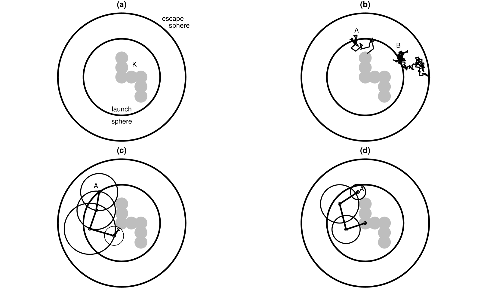
Let be the (solid) unit ball in and then is the ball with center and radius . Throughout we assume that there are two radii . See Figure 1(a) for the case. It is assumed that the object is contained in the launch ball . The larger sphere of radius will be called the escape sphere; it is used in deciding whether a random walk escapes to infinity without hitting .
For both Brownian and stable paths a probabilistic description of where the walk exits or enters a ball is known. Since Brownian motion has continuous sample paths, the enter or exit location will be on the surface of the ball with probability 1. However, when , the paths are discontinuous and the hitting location will be strictly inside or outside the ball with probability 1; see Blumenthal et al. [4]. If we start a path at a finite location, the Appendix shows the distribution of hitting locations for a ball.
To exactly simulate the hitting from infinity location, we need to choose an appropriate finite starting distribution. The correct starting location is based on where a walk starting at infinity hits the launch ball. For the Brownian case, this means the starting location is on the launch sphere and that distribution is uniform; for cases, the starting location is distributed across the launch ball according to the equilibrium distribution for the launch ball, e.g., equation (9) in the Appendix.
2.1 Stable random walks
Mansfield et al. [22] introduced an algorithm for computing the 2-capacity in the special case where and based on hitting the set with simple random walk trajectories. As noted above, these paths start uniformly on a launch sphere that contains . We next describe a natural extension of this algorithm to general and dimensionality . Throughout we assume to guarantee that the Lévy flights are transient (see Appendix for definition). The method requires two basic elements: a way to simulate isotropic stable random vectors and to be able to compute the probability of hitting a ball given that we start at an exterior point. The Appendix describes how to do both of these for -stable motion in , .
Let be a scale variable for the step size, i.e. each step of the random walk will have characteristic function
| (2) |
This isotropic stable process is described in Chapter 3 of Sato [36]. Let be a hitting tolerance, i.e. we will consider that the walk has hit if the distance between a point and is less than or equal . Typically ; the first inequality implies that the “thickening” of is small compared to the typical step size and the second inequality implies that the typical step size is small compared to the size of the object. We generate a path according to the following algorithm, see Figure 1(b).
-
1.
Pick a starting point . If , this means pick uniformly on the launch sphere; if , this means pick according to the equilibrium distribution on the launch ball using equation (9) below.
-
2.
Generate a step with distribution given by equation (2) and compute a new location .
-
3.
If , compute the probability of a walk hitting the launch ball starting at . (Recall that the process is transient.) With probability , declare that this walk will escape to infinity without ever hitting the launch ball (and therefore not hit ) and we stop this path. Otherwise, compute a new location by simulating a hitting location in the launch ball by a walk starting at the current location as described in the Appendix.
-
4.
If is within of , declare the current location to be a hit. Otherwise, go to step 2.
We note that since a stable process generally jumps into the interior of a set, we can set for the kinds of sets considered here. For thin sets, say fractals, we may want to use an to effectively “thicken” , but the influence of this on the final results should be carefully examined.
This process is repeated times and a count of number of hits of and their locations are saved.
2.2 Walk-On-Spheres method for Brownian motion
When , Muller [26] introduced a faster method to simulate from the hitting distribution of a general set . The continuity of Brownian paths guarantees that a path can only leave a ball by crossing its boundary, a sphere. Furthermore, the rotational symmetry means that the distribution of exit points is uniform on the sphere. So rather than simulate many steps, this method chooses random exit points on a sequence of (random) spheres, see Figure 1(c). This is called the Walk-On-Spheres method, abbreviated WOS. Here are the steps in the algorithm to generate a single path.
-
1.
Pick a point uniformly from the launch sphere.
-
2.
Compute distance between and .
-
3.
Pick a new point uniformly on the sphere of radius centered on
-
4.
If , return as the hitting location.
-
5.
Otherwise, set .
-
6.
If , compute the probability of a walk starting at hitting the launch ball. With probability , declare that this walk will escape to infinity without ever hitting the launch ball (and therefore not hit ). Otherwise, go to step 2.
2.3 Walk-In-and-Out-of-Balls for stable path processes
When , the Walk-On-Spheres method cannot be used because the stable process has jumps and will exit a ball not on the boundary, but on some point exterior to the ball. Blumenthal et al. [4] give expressions for the distribution of these exit point for -stable processes with . They also give the probability of hitting a ball when starting from some exterior point and what the hitting location is on the interior of the ball. These expressions are given in the Appendix.
The approach below extends the work of Kyprianou et al. [19]. That work considers the interior problem: a stable process starts at a point , and the paths are followed until they exit . In contrast, we are concerned with the exterior problem: in which we start at a point , and propogate the path until it hits . There are several key differences between [19] and the method proposed here; we describe them below.
Our approach generates a sequence of points that are outside a sequence of balls, with a check to avoid drifting too far from the object that sometimes returns us to the launch ball . We call this method the Walk-In-and-Out-of-Balls method, abbreviated WIOB. The steps of the method are given below, see Figure 1(d) to visualize the steps.
-
1.
Pick a point on the launch ball according to the equilibrium distribution in equation (9).
-
2.
Compute the distance = distance between and .
-
3.
Simulate an exit location from the ball of radius centered on .
-
4.
If , return as the hitting location.
-
5.
Otherwise, set .
-
6.
If , compute the probability of a walk starting at hits the launch ball. With probability , declare that this walk will escape to infinity without ever hitting the launch ball (and therefore not hit ) and stop this iteration. Otherwise, simulate reentering the launch ball at a new point and go to step 2.
There are two advantages of this method. First, like the WOS method for Brownian motion, it is generally more efficient. Instead of many small steps, the focus on leaving a ball means each WIOB step is larger and faster than many small steps. Second, WIOB allows a miss of the object that could occur with a jump that the WOS method does not allow. The chance of this happening is small, because small jumps are more likely, but the probability of a large step increases as decreases.
We now describe differences between [19] and WIOB. Both methods rely on the key results in [4], but have different objectives. [19] is interested in simulating paths to compute a solution of a fractional diffusion equation and do not consider capacity, which is the main focus of this paper. They fix a starting location , whereas we start at a random location, which we specified above, chosen to exactly simulate hitting from infinity in step 1. They do not have to deal with transience and the possibility that the process never hits , whereas we deal with this possibility in step 6. Simulating the return to the launch ball uses the density from the Appendix. The straightforward way of doing this with simple rejection is increasingly less efficient as the point becomes closer and closer to the launch ball. Devroye and Nolan [8] have developed algorithms for exactly simulating locations for entering or leaving a ball that are uniformly bounded for all starting locations . We note that these methods work for all and any dimension , enabling calculating standard capacity and Riesz capacity. This enables new applications in dimension not equal to 3.
3 Estimating from hitting locations
Throughout this section is a fixed compact set. We will use the results of the previous section to compute an estimate of and give confidence intervals for this estimate.
3.1 Electrostatic capacity from Brownian paths
For electrostatic capacity, e.g. and , then for any ,
| (3) |
Based on this result, it can be shown that if is any compact set,
| (4) |
3.2 Riesz capacity from -stable sample paths
When , the situation is more complicated. For a ball, there is an expression for the hitting probability that is the analog of equation (3), see equation (8) in the Appendix below. However, there is no known relationship between hitting probability and -capacity for a general set .
The proposed solution is to run simulations of the WIOB method to obtain hitting locations in the set . Using these hitting locations gives an empirical distribution that is an approximation to the equilibrium measure of the set. The straightforward approach is to evaluate the energy integral (1) with a sum, i.e.
where is the number of distinct non-diagonal pairs in .
Unfortunately, there are two problems with this seemingly straightforward approach. The first problem is that this sum is a numerically unreliable way to approximate the energy integral because the integrand in (1) has a singularity on the diagonal . With a sample, if , one or more terms in the sum above can dominate the sum, leading to a poor estimate of . The second problem is that the terms in this sum are dependent, so it is not straightforward to get a confidence interval for such an estimate. Below, we describe a way to split the sample into two groups and use different estimators form the groups in a way that gives less volatile estimates of capacity and valid confidence intervals.
An equivalent way of viewing this is to define the random variable , where and are independent copies with distribution . Then , the expectation of . Points that are close to each other on correspond to large values of . In probabilistic terms, is a heavy-tailed variable and therefore estimating the mean can be unreliable. And contrary to most statistical estimates, the larger the sample, the more likely it is that we will see very large values of and get a less reliable estimate of . Furthermore, in cases where the , , but the sample mean will never lead to a value of .
We propose a method to approximate that detects the case, gives reliable estimates of when it is finite, and in this later case, gives a large sample confidence interval for , and thus a confidence interval for . Start with a sample of hitting locations and define , . Pick a threshold for determining which of these values is large. A convenient choice is to define to be an upper quantile of , e.g. for some value . Split the integral for into two pieces:
We will estimate using of the samples and by a tail estimator based on the remaining values.
For , define . This is a bounded random variable, so necessarily has a finite mean and variance. Then, define the sample analogue for and the following terms:
Then is a U-estimator of . The variance term is used below to get a confidence interval for .
For , we assume that the upper tail of has a power decay:
| (5) |
To estimate , select values from , where (a) , (b) there is at most one value selected from each row of the matrix, and (c) there is at most one value selected from each column of the matrix. Since we are only choosing the from , the are independent of the used in estimating , the values are independent of and because of conditions (b) and (c) above, the values are independent of each other. Hence, the values are an i.i.d. sample from the upper tail of . We use the Hill estimator for the tail decay :
In the simulations we have run, we’ve observed when or ( and ), in which case Var. Assume that the tail approximation (5) is exact for . Then has an upper tail density and necessarily . Then the value of is and the estimate of is
The energy integral estimate is , and the -capacity estimate is . Note that if , the sum and .
3.3 Confidence interval for -capacity estimates
The ZENO program has a method of deriving large sample confidence intervals when and . Large sample confidence intervals based on the normal distribution are described next for arbitrary and .
We assume , so . First, the variance of will be estimated. By the way the sample is split above, the two estimators and are independent, so Var = Var + Var. The standard theory of U-statistics, e.g. Chapter 12 of van der Vaart [43], gives an estimator of the variance of that is sometimes negative. (This possibility is mentioned on page 419 of Schucany and Bankson [38]; surprisingly, this can happen with large samples, e.g. .) To avoid that problem, we use the modified variance estimator of Sen [39]: namely
With appropriate regularity conditions, the Hill estimator based on the largest values is approximately N, see page 304 of Resnick [32]. Using the delta method on shows that is approximately N, with . Thus is approximately N, where . Finally, using the delta method again, the estimate of capacity is approximately N, where . Hence, a large sample confidence interval is given by .
4 Implementation and numerical examples
The Walk-In-and-Out-of-Balls method has been implemented in R, a free open source programming language, see R Project [31]. It allows general and some basic types of target objects: unions of balls, unions of cubes, unions of rectangular solids, and cylinders. The simulations in this sections shows some examples of estimated -capacity for several objects in different dimensions.
4.1 of a ball in
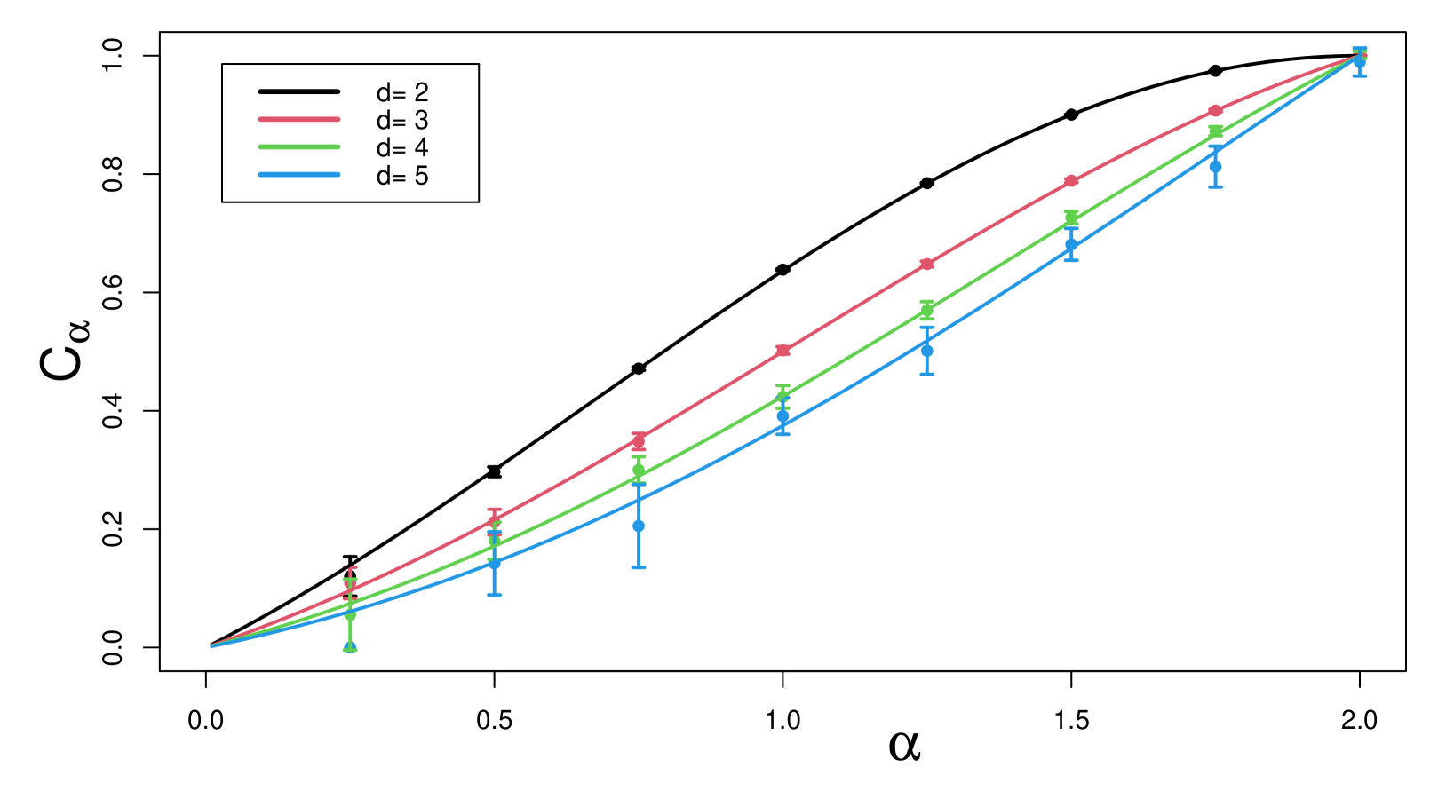
The only case where an exact formula is known for the -capacity of a -dimensional set is for a ball; it is given in equation (7) below. Here we focus on the unit ball in dimension . This first simulation used the WIOB method to estimate -capacity and then compares those estimates to the theoretical values. Figure 2 compares these numerical estimates to the exact theoretical values in equation (7) in the Appendix. Since the exact -capacity of a sphere is known, we may gauge the accuracy of the simulation by the deviation between estimates based on simulation and analytic, exact values. For example, when , the confidence interval width varies from 0.0948 when to 0.00318 when . Increasing the sample size will improve the accuracy.
4.2 of solid and hollow cubes
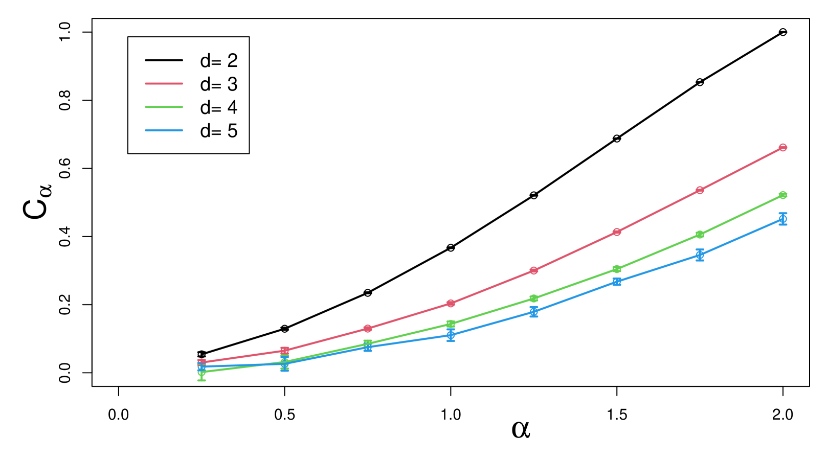
First let be the solid cube . Figure 3 shows estimated of a these cubes in dimensions 2, 3, 4, and 5 as a function of . In particular, the estimated value of this capacity when and is using WIOB with . This compares to previous estimates of 0.663 in Mansfield et al. [22], using 4.7 billion trajectories in Given et al. [12] and in Hwang et al. [14]. The particular virtue of the path integration method for estimating capacity is that it allows for highly precise estimates in comparison with other methods such as finite element methods when a large number of trajectories is employed.
Separate simulations, not shown here, demonstrate that the method introduced here satisfies the scaling property given in equation (6) in the Appendix: for . So these capacity values for unit cubes give the capacity of any cube.
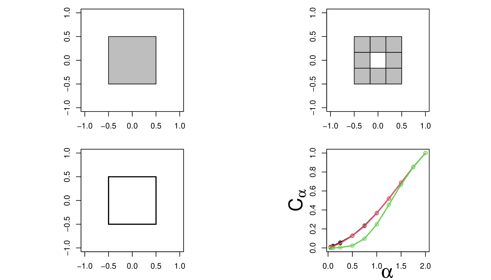
Since non-Gaussian stable processes exhibit discontinuous path displacements, their hitting locations are not restricted to the surface of an object. This class of erratic path processes can thus penetrate through the boundary before they hit . So unlike 2-capacity, the -capacity of a hollow object can differ from the -capacity of a solid object with the same bounding surface. To examine this effect in 2-dimensions, we look at a solid and hollow squares. Figure 4 shows these three regions: the first (upper left) is a single, solid square (top left), the next is a hollow square with a thick wall of width 1/3 (top right), and one with a thin wall of width 1/100 (bottom left). The bottom right plot shows the estimated -capacity of the three objects for a range of in (0,2]. The black curve for the solid cube is mostly covered by the thick walled curve in red, showing that it is difficult to get through a thick barrier when most of the jumps of a stable process are small. For the thin-walled cube, the green curve does diverge from the other two curves, and this difference is larger when is small. In theory, this allows one to distinguish between solid and hollow objects with the same surface, something not possible with Brownian motion.
4.3 of a solid rectangular bar in three dimensions
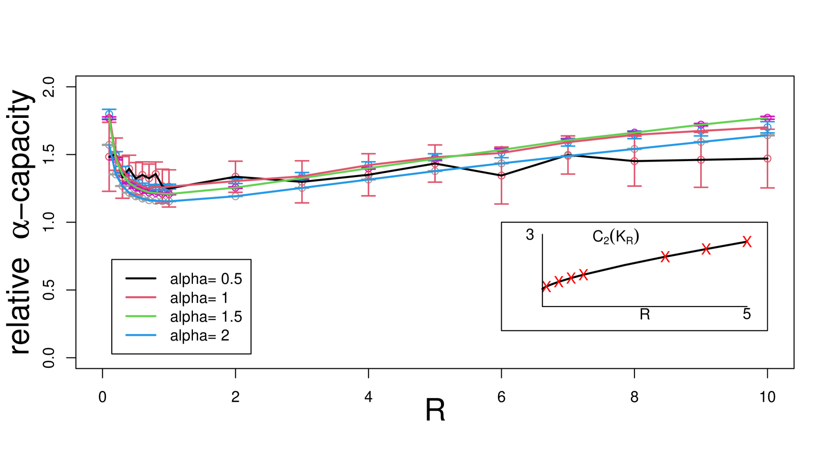
Here we consider an anisotropic example in : . This is a solid bar with length and cross section a square of area 4, so it has volume . As varies away from 1 in either direction, the set gets more and more anisotropic. Since the volume of increases with , we normalize each capacity estimate by dividing it by the -capacity of a ball with the same volume as . This type of dimensionless ratio, the relative capacity, provides valuable information about the shape of a region, e.g., Polya and Szego [29]. Figure 5 shows the results of simulating hitting locations and computing capacity for a range of and . The increase in relative capacity near is caused by the fact that decreases to 0 more slowly than (ball with the same volume as . The subplot in the figure shows that the WIOB method agrees closely with the ZENO program when .
Recently, there has been great interest in developing a ”fingerprint” of the shape of objects through the calculation of the eigenvalues of the region based on solving the wave equation for objects of general shape, e.g. Reuter et al. [33] and Peincke et al. [28]. The eigenvalue spectrum is clearly advantageous to other shape functionals as it involves the calculation of an infinite (large number) of numbers to specify object shape. The capacity likewise involves a “spectrum” of values that might better quantify object shape. We note that the relative capacity obeys the same isoperimetric property (see the Appendix), i.e., the -capacity quantity is minimized by a sphere of all regions K of a fixed volume. It is this isoperimetric property that makes the relatively capacity of interest in shape classification and discrimination problems, as discussed for the 2-capacity and other shape functionals having this fundamental isoperimetric property.
4.4 of a thin “coin”
Here we consider a thin “coin” . Since will be small, is approximately a two dimensional set sitting inside of . This example illustrates two topics: using capacity to find Hausdorff dimension and subordination.
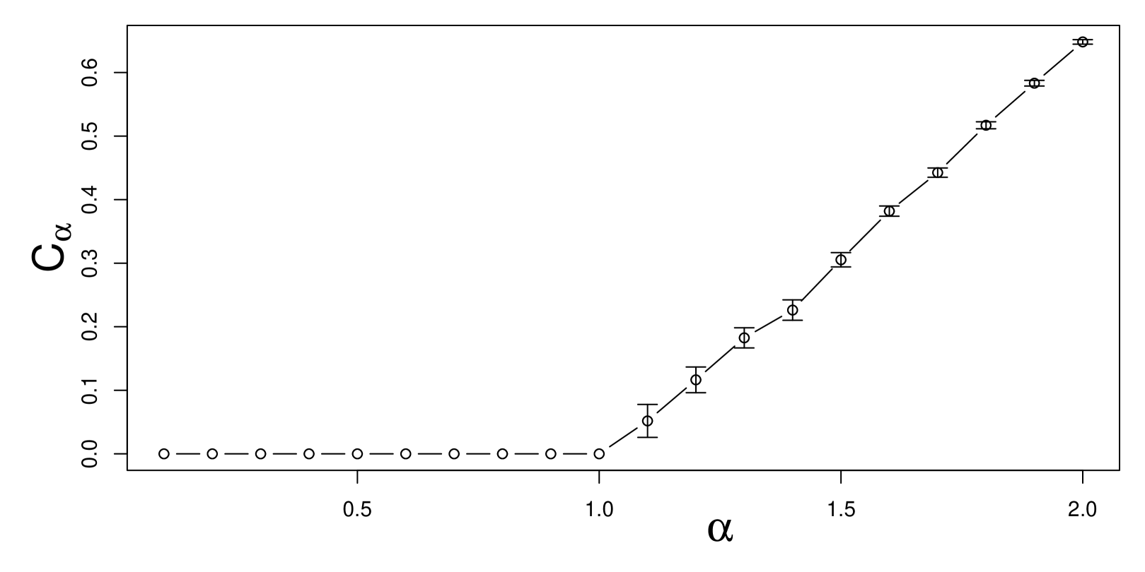
For the first topic, we calculate the -capacity of the coin in three dimensions for a range of values and see where the capacity reaches 0. Figure 6 shows the result, where defines a condition at which the -capacity reaches 0. This behavior arises because the Hausdorff dimension of the coin is . (This conclusion follows from work by Taylor [41], using a lemma of Frostman [11] for the calculation of Hausdorff dimension of Brownian motion paths and other “fractal” sets. That work shows that the value of where reaches 0 rigorously defines the Hausdorff dimension of .) Correspondingly, the 2-capacity of the thin coin vanishes in four dimensions in the case of Brownian motion, since the thin ”coin” and Brownian motion have the same Hausdorff dimension, see Taylor [41], Dvoretzky et al. [10], and McKean [23].
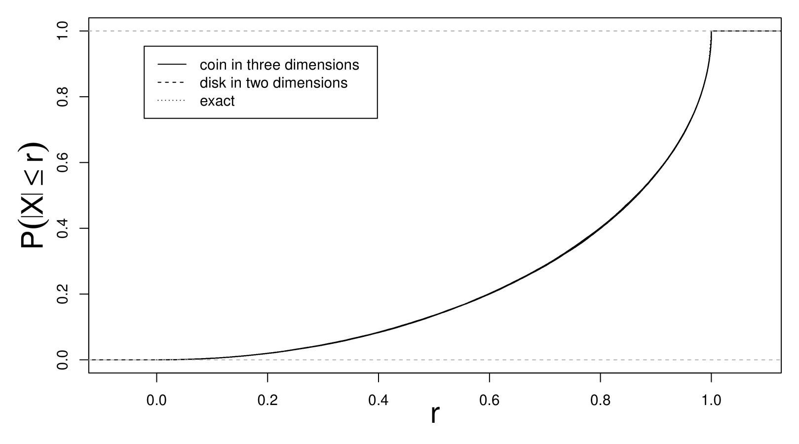
For the other topic, consideration of the hitting locations of Brownian motion () in on an infinitely thin “coin” provides an example of subordination, the reduction of Brownian motion to a Lévy type process by “decimating” the Brownian motion at random time points. In particular, the times at which the random walk in three dimensions hits a disc defines a random Cantor set of time points of fractal dimension 1/2 (the subordinating set) and the path process connecting the original random walk path positions at these time points defines a Cauchy process () where the paths are then limited by construction to the unit disk in . We use the WOS method for Brownian motion to generate a sample hitting distribution of the unit disk. We then perform a separate WIOB simulation for the unit disk in with an path process and determine hitting locations . To compare these to each other, the radial symmetry says it suffices to compare the distributions of univariate radii (ignoring the small first coordinate) to univariate . Figure 7 shows the cumulative distributions of these radii. Also on the plot is a third curve, which is the exact cumulative distribution of the radii of the Cauchy equilibrium distribution derived from (9) with and . The view that the two dimensional Cauchy process is just a subordinated version of the three dimensional Brownian path process, as described above, implies that the hitting distributions of the disk should then be the same. We find that this might arise naturally when viewing the dynamics of a higher dimensional Brownian process in some space of reduced dimension. We do not claim this is a universal explanation, but this may be a common mechanism.
4.5 Coverage probability for confidence intervals
To assess the performance of the confidence interval method of Section 3.3, we simulated runs with the unit ball in dimension and three values. The exact value of the -capacity is known in this case, so we counted how many of the 500 simulated 95% confidence intervals contained the exact value. For , the observed coverage probability was 0.992; for , the observed coverage probability was 0.966; and for , the observed coverage probability was 0.958. The other parameters are , , , , . The observed coverage probabilities are high, apparently due to the large values of . It appears that even with the truncation at values of above , the large values of inflate the estimator . This will be investigated in future work. Presently, observe that the confidence intervals are conservative, and that a larger simulation can be used to get smaller confidence intervals.
5 Conclusion
This work demonstrates that it is possible to precisely estimate -capacity for general sets in -dimensions when . In particular, it also novel in that it estimates standard electrostatic capacity in dimension . Below, we first discuss the parts of the algorithm that are slow, and then discuss some other applications of this approach.
The programs used here are written in R which is an interpreted language, so would be faster if recoded in C/C+. It is also straightforward to parallelize the simulations of the hitting locations, because each path is independent of all others. The run time is quicker if the object is centered near the origin and if the launch ball is the smallest centered ball that contains .
Generating the hitting locations is currently slow for complicated objects, because the R code computes the distance between the current location and in step 2 of the WIOB method. If is a polymer modeled by the union of thousands of beads, this is very slow. The contribution of Juba et al. [16] was the development of an optimized data structure for that allows the efficient determination of which beads are close to , greatly reducing the number of computations required and a corresponding substantial reduction of the required computation time to obtain results having a prescribed uncertainty. This technique can be applied here to speed up simulations.
The time consuming part of the -capacity estimation is the computation of , which is quadratic in . Calculation of is of order . The algorithm is also memory intensive, requiring memory locations for the matrix . It is possible to improve on this and if time is not a concern, one can keep just the hitting locations and compute entries of the matrix as needed.
This approach can be used to give an approximate solution to fractional diffusions, see Kyprianou et al. [19]. In this context, we have described the steps needed to solve the exterior problem, i.e. starting a fractional diffusion outside of and running the path until it hits . These same tools can be adapted to solve the interior problem where we start inside and run the process until it leaves the set using the WIOB method. Hunt et al. [13] discuss a potentially important application of this type of calculation to modeling the velocity field of high Reynolds number pipe flow.
Finally, because the parameter can be varied in the interval , we obtain a “spectrum” of capacity estimates for any set . Dividing these -capacity values by the capacity of a ball having the same volume as gives shape information. Such a “spectrum” should be useful in shape discrimination. These values can provided information about the interior of sets, as in the cases of hollow squares considered in Section 4.2. In the case of fractal sets, it should be possible to estimate the Hausdorff dimension by varying and finding the value at which . This approach has long been used in analytic estimates of fractal sets such as Brownian motion through the use of upper and lower bounds as in Taylor [42], but this method has apparently never been implemented numerically using path integration methods. We expect this method of calculating fractal dimension to be quite general and capable of precise dimension estimates.
Appendix A Properties of capacity and stable processes
In this section we collect technical results on stable processes and capacity that are used above. We do not prove these results, only give references to where these facts can be found. General information on stable distributions can be found in Nolan [27] and information on stable processes can be found in Samorodnitsky and Taqqu [35], Sato [36], and Bogdan et al. [5]. Landkof [20] gives the basic properties of -capacity in Chapter 2.
- Translation and scaling.
-
If is any compact set, any scale , and shift ,
(6) Note that in only two cases: electrostatic capacity () when or Cauchy capacity () when .
- Transcience/recurrence.
-
For , an -stable motion is recurrent if , transient if . See Sato [36], Chapter 7. The method described here for calculating -capacity can only be used in the transient case.
- -capacity of a ball.
-
Let be the unit ball. Then for any shift and scale
(7) This is given on page 111 of Takeuchi [40].
- Isoperimetric and symmetrization properties
-
For all regions of fixed volume and for all , the capacity is minimized for a sphere. This was first proved by Watanabe [45]. We may more generally expect objects having greater symmetry to have a lower capacity. See Betsakos [3], [2], and Mendez-Hernandez [24]Kojar [17] for proofs and discussions of these facts.
- Subadditivity.
-
For compact Borel sets , . See [20], Chapter 2.
- Hitting probability for a ball.
-
A stable motion hits the ball if and only if the shifted and scaled process hits the unit ball . Likewise, leaves the ball if and only the shifted and scaled process leaves the unit ball . Because of this, we can restrict ourselves to considering entering and leaving the unit ball. For the unit ball and starting at with ,
(8) where is the cumulative distribution function of a Beta distribution with parameters and . This follows from a change of variables in Corollary 2 of Blumenthal et al. [4].
This can also be expressed as , where is the first hitting time. A series expansion for the exact probability of hitting the unit ball is
where the coefficients are given by and recursively for by
This follows from the Taylor series expansion for the incomplete Beta function around 0. If and , and all other coefficients are 0, so . When , some algebra shows all and they are strictly decreasing, so a truncated series is always a lower approximation for the probability of hitting a ball.
For a ball of arbitrary center and radius , when is not in the ball, scaling shows that in the transient case
- Hitting location for a ball.
-
In the Brownian case, the distribution of the hitting location starting from outside the unit ball is concentrated on the surface of the sphere. When , the hitting location for the ball is the nearest endpoint. When , it has density given by the Poisson kernel:
see Mörters and Peres [25], Theorem 3.44. When , Blumenthal et al. [4] showed that an stable motion starting at outside the unit ball has hitting density for
where . For a ball of center and radius , shifting and scaling the above formulas can be used.
Devroye and Nolan [8] show how to efficiently simulate from this density. That method assumes that is on the axis for simplicity. To handle a general starting location , see below.
- Hitting location for the complement of a ball.
-
In part of the WIOB method, an stable process is started at a point on the interior of a ball and it is run until it exits the ball to a point . Because of the shifting and scaling properties, it suffices to consider the centered unit ball.
When , use , where is uniform on the unit sphere and Beta(). When , duality can be used. [6] call this the Kelvin transform. Reflect the point across the boundary sphere: . Since is outside the ball, we can run a stable process starting at until it hits the ball at some point . Then reflect to get to get the desired random vector.
- Generating vectors uniformly distributed on .
-
If has independent components, is uniformly distributed on the unit sphere .
- Generating isotropic stable vectors.
-
Suppose , , and is a positive -stable random variable with scale and zero shift. This can be directly simulated using the method in Chambers et al. [7]. In the case the formula is
where is uniformly distributed on and is an independent exponential r.v. with mean 1. If has independent components, then is an isotropic stable random vector with characteristic function (2).
- Equilibrium measure for a ball.
-
When , Takeuchi [40], page 111, gives the density of the equilibrium distribution for the unit ball as
(9) This can be simulated by taking where the are i.i.d. and computing
where Beta().
When , the equilibrium measure is uniform on the sphere, which can be simulated using the method above: .
- Arbitrary starting locations
-
The methods described in Devroye and Nolan [8] for simulating hitting a ball assume the stable motion starts at a point on the -axis. For a general starting position find a rotation matrix such that , run the algorithm with to get a hitting location , and rotate back to get . One fast way to find such a rotation is to use a sequence of Given’s rotations to successively zero out the -th component of , then the -th component, etc. Then apply these rotations in reverse to get . Since can be computed by just calculating , is not needed for this algorithm, we only need to find .
The algorithms to compute and only take steps since the matrices are sparse. A third function is provided to compute a rotation matrix that takes any non-zero vector to any other non-zero vector by composing a rotation from an original vector to the -axis, then a rotation from the -axis to the desired direction.
- More information from simulations
-
The code implements hitting locations in both the simple random walk method of Section 2.1 and WIOB method of Section 2.3. In this paper, we have only used the final hitting location of a stable motion, but the program gives the option of saving the path, which may be of interest in solving other problems, e.g. fractional diffusions.
Acknowledgments
The authors would like to thank David Gerard of American University for discussions about U-statistics, Renming Song of the University of Illinois for alerting us to Theorem 2 in [30], and two reviewers whose comments improved the paper.
References
- [1] B. A. P. Betancourt, S. J. Florczyk, M. Simon, D. Juba, J. F. Douglas, W. Keyrouz, P. Bajcsy, C. Lee, and C. G. Simon, Effect of the scaffold microenvironment on cell polarizability and capacitance determined by probabilistic computations, Biomedical Materials, 13 (2018), p. 025012.
- [2] D. Betsakos, Addendum to “Symmetrization, symmetric stable processes, and Riesz capacities”, Transansactions of the American Mathematical Society, 356 (2004), p. 3821.
- [3] D. Betsakos, Symmetrization, symmetric stable processes, and Riesz capacities, Transansactions of the American Mathematical Society, 356 (2004), pp. 735–755.
- [4] R. M. Blumenthal, R. K. Getoor, and D. B. Ray, On the distribution of first hits for the symmetric stable processes, Transactions of the American Mathematical Society, 99 (1961), pp. 540–554.
- [5] K. Bogdan, T. Byczkowski, T. Kulczycki, M. Rysnar, R. Song, and Z. Vondraček, Potential Analysis of Stable Processes and its Extensions, Springer, Berlin, 2009.
- [6] K. Bogdan and T. Zak, On Kelvin transformation, J Theor Probab, 19 (2006), p. 89–120.
- [7] J. Chambers, C. Mallows, and B. Stuck, A method for simulating stable random variables, Journal of the American Statistical Association, 71 (1976), pp. 340–344. Correction in JASA 82 (1987), 704.
- [8] L. Devroye and J. P. Nolan, Random variate generation for the first hit of the symmetric stable process in , Preprint, (2022).
- [9] J. F. Douglas, H.-X. Zhou, and J. B. Hubbard, Hydrodynamic friction and the capacitance of arbitrarily shaped objects, Physical Review E, 49 (1994), pp. 5319–5331.
- [10] A. Dvoretsky, P. Erdös, and S. Kakutani, Double points of paths of Brownian motion in -space, Acta Scientiarum mathematicarum Univ. Szeged., 12 (1950), pp. 75–81.
- [11] O. Frostman, Potentiel d’équilibre et capacitié des ensembles, avec quelques applications a la théorie des fonctions, Medd. Lunds University Mat. Semin., 3 (1935).
- [12] J. A. Given, J. B. Hubbard, and J. F. Douglas, A first-passage algorithm for the hydrodynamic friction and diffusion-limited reaction rate of macromolecules, Journal of Chemical Physics, 106 (1997), pp. 3761–3771.
- [13] F. Y. Hunt, J. F. Douglas, and J. Bernal, Probabilistic computation of Poiseuille flow velocity fields, Journal of Mathematical Physics, 36 (1995), pp. 2386–2401.
- [14] C.-O. Hwang and M. Mascagni, Electrical capacitance of the unit cube, Journal of Applied Physics, 95 (2004), pp. 3798–3802.
- [15] D. Juba, D. J. Audus, M. Mascagni, J. F. Douglas, and W. Keyrouz, Zeno: Software for calculating hydrodynamic, electrical, and shape properties of polymer and particle suspensions, Journal of Research of National Institute of Standards and Technology, 122 (2017).
- [16] D. Juba, W. Keyrouz, M. Mascagni, and M. Brady, Acceleration and parallelization of zeno/walk-on-spheres, Procedia Computer Science, 80 (2016), pp. 269–278.
- [17] T. Kojar, Brownian motion and symmetrization, 2015, https://arxiv.org/abs/1505.01868.
- [18] V. I. Kruglikov, Capacity of condensers and spatial mappings quasiconformal in the mean, Mathematics of the USSR-Sbornik, 58 (1987), p. 185.
- [19] A. E. Kyprianou, A. Osojnik, and T. Shardlow, Unbiased ‘walk-on-spheres’ Monte Carlo methods for the fractional Laplacian, IMA Journal of Numerical Analysis, 38 (2017), pp. 1550–1578.
- [20] N. S. Landkof, Foundations of modern potential theory, Springer-Verlag, New York-Heidelberg, 1972. Translated from the Russian by A. P. Doohovskoy, Die Grundlehren der mathematischen Wissenschaften, Band 180.
- [21] M. L. Mansfield and J. F. Douglas, Improved path integration method for estimating the intrinsic viscosity of arbitrarily shaped particles, Phys. Rev. E, 78 (2008), p. 046712.
- [22] M. L. Mansfield, J. F. Douglas, and E. J. Garboczi, Intrinsic viscosity and the electrical polarizability of arbitrarily shaped objects, Phys. Rev. E, 64 (2001), p. 061401.
- [23] H. P. J. McKean, Hausdorff-Besicovitch dimension of Brownian motion paths, Duke Mathematical Journal, 22 (1955), pp. 229 – 234.
- [24] P. J. Méndez-Hernández, An isoperimetric inequality for Riesz capacities, Rocky Mountain Journal of Mathematics, 36 (2006), pp. 675 – 682, https://doi.org/10.1216/rmjm/1181069473.
- [25] P. Mörters and Y. Peres, Brownian motion, vol. 30 of Cambridge Series in Statistical and Probabilistic Mathematics, Cambridge University Press, Cambridge, 2010.
- [26] M. E. Muller, Some continuous Monte Carlo methods for the Dirichlet problem, The Annals of Mathematical Statistics, 27 (1956), pp. 569–589.
- [27] J. P. Nolan, Univariate Stable Distributions - Models for Heavy Tailed Data, Springer Verlag, New York, 2020. Chapter 1 online at https://edspace.american.edu/jpnolan.
- [28] N. Peinecke, F.-E. Wolter, and M. Reuter, Laplace spectra as fingerprints for image recognition, Computer-Aided Design, 39 (2007), pp. 460–476, https://www.sciencedirect.com/science/article/pii/S0010448507000085.
- [29] G. Pólya and G. Szegö, Isoperimetric Inequalities in Mathematical Physics, Annals of Mathematical Studies, Princeton University Press, 1951.
- [30] S. C. Port, On hitting places for stable processes, Ann. of Math. Stat., 38 (1967), pp. 1021–1026.
- [31] R Core Team, R: A Language and Environment for Statistical Computing, R Foundation for Statistical Computing, Vienna, Austria, 2022.
- [32] S. I. Resnick, Heavy-tail phenomena, Springer Series in Operations Research and Financial Engineering, Springer, New York, 2007. Probabilistic and statistical modeling.
- [33] M. Reuter, F.-E. Wolter, and N. Peinecke, Laplace–Beltrami spectra as ‘Shape-DNA’ of surfaces and solids, Computer-Aided Design, 38 (2006), pp. 342–366, https://www.sciencedirect.com/science/article/pii/S0010448505001867. Symposium on Solid and Physical Modeling 2005.
- [34] M. Riesz, Intégrales de Riemann-Liouville et potentiels, Acta Sci. Math. Szeged., 9 (1938), pp. 1–42.
- [35] G. Samorodnitsky and M. Taqqu, Stable Non-Gaussian Random Processes, Chapman and Hall, New York, 1994.
- [36] K. Sato, Lévy Processes and Infinitely Divisible Distributions, Cambridge University Press, 1999.
- [37] M. Schiffer and G. Szegö, Virtual mass and polarization, Trans. Amer. Math. Soc., 67 (1949), pp. 130–205.
- [38] W. R. Schucany and D. M. Bankson, Small sample variance estimator for U-statistics, Austral. J. Statist., 31 (1989), pp. 417–426.
- [39] P. K. Sen, On some convergence properties of U-statistics, Calcutta Statistical Assocition Bulletin, 10 (1960), pp. 1–18.
- [40] J. Takeuchi, On the sample paths of the symmetric stable processes in spaces, J. Math. Soc. Japan, 16 (1964), pp. 109–127.
- [41] S. J. Taylor, The -dimensional measure of the graph and set of zeros of a Brownian path, in Mathematical Proceedings of the Cambridge Philosophical Society, vol. 51, Cambridge University Press, 1955, pp. 265–274.
- [42] S. J. Taylor, On the connexion between Hausdorff measures and generalized capacity, Mathematical Proceedings of the Cambridge Philosophical Society, 57 (1961), pp. 524––531.
- [43] A. W. van der Vaart, Asymptotic Statistics, Cambridge University Press, 1998.
- [44] F. Vargas-Lara, M. L. Mansfield, and J. F. Douglas, Universal interrelation between measures of particle and polymer size, The Journal of Chemical Physics, 147 (2017), p. 014903.
- [45] T. Watanabe, The isoperimetric inequality for isotropic unimodal Lévy processes, Z. Wahrsch. Verw. Gebiete, 63 (1983), p. 487–499.