Computational Image Enhancement for Frequency Modulated Continuous Wave (FMCW) THz Image
Abstract
In this paper, a novel method to enhance Frequency Modulated Continuous Wave (FMCW) THz imaging resolution beyond its diffraction limit is proposed. Our method comprises two stages. Firstly, we reconstruct the signal in depth-direction using a -envelope, yielding a significant improvement in depth estimation and signal parameter extraction. The resulting high precision depth estimate is used to deduce an accurate reflection intensity THz image. This image is fed in the second stage of our method to a 2D blind deconvolution procedure, adopted to enhance the lateral THz image resolution beyond the diffraction limit. Experimental data acquired with a FMCW system operating at 577 GHz with a bandwidth of 126 GHz shows that the proposed method enhances the lateral resolution by a factor of 2.29 to 346.2um with respect to the diffraction limit. The depth accuracy is 91um. Interestingly, the lateral resolution enhancement achieved with this blind deconvolution concept leads to better results in comparison to conventional gaussian deconvolution. Experimental data on a PCB resolution target is presented, in order to quantify the resolution enhancement and to compare the performance with established image enhancement approaches. The presented technique allows exposure of the interwoven fibre reinforced embedded structures of the PCB test sample.
Keywords Terahertz, Frequency Modulated Continuous Wave (FMCW), resolution enhancement, deconvolution, parameter extraction
1 Introduction
Since its original inception in the early nineties [1], THz imaging has demonstrated a very large potential for contact-free analysis, nondestructive testing and stand-off detection in a wide variety of application fields, such as semiconductor industry, biology, medicine, material analysis, quality control, and security [2, 3, 4]. In many of these application fields, THz imaging is competing with established imaging methodologies, such as optical inspection or X-ray imaging. Compared with imaging in the optical or X-ray parts of the electromagnetic spectrum, THz imaging is significantly limited in its spatial resolution due to the substantially longer wavelength of the associated frequencies.
A wide range of technological approaches to realize THz imaging systems have been demonstrated, including femtosecond laser based scanning systems [1, 5], synthetic aperture systems [6, 7], and hybrid systems [8]. Several of these approaches using pulses or using frequency modulated THz signals, allow to sense temporal or phase shifts to the object’s surface, making 3D THz imaging possible.
Despite the fact that in most of these approaches THz imaging is performed close to the diffraction limit, the comparatively low spatial resolution associated with the THz radiation wavelengths significantly hampers the application range. There is a huge interest to increase the spatial resolution of this approach beyond the diffraction limit, in order to make this technique competitive in comparison to established methods such as X-ray imaging [9].
THz imaging below the diffraction limit is an emerging area [3], which can roughly be classified into two alternatives: by system enhancements or by computational approaches. System enhancements include for example, interferometric sensing [10] to increase the depth sensitivity in THz time-of-flight imaging, or near-field sensing approaches [11] which demonstrate a nanometer scale lateral resolution by circumventing the diffraction limit. Computational image enhancement techniques aim at improving the resolution by utilizing numerical procedures and additional signal or system information, e.g. from overlapping oversampled THz imaging signals, without introducing additional equipment effort and cost.
Depending on the THz image acquisition mode, there are several alternative approaches for computational image enhancement. THz imaging superresolution (also referred to as high-resolution or image restoration) is often associated to spatial resolution enhancement in the xy-direction [12, 13, 14, 15, 16]. In contrast, depth resolution enhancement is associated to improvement in azimuth direction (z-direction) [17, 18, 19].
In this paper, we propose a novel method to enhance THz image resolution beyond diffraction limit, attaining a lateral (xy) resolution increase and a depth (z) accuracy increase. The concept is demonstrated for a Frequency Modulated Continuous Wave (FMCW) THz scanning system operating at GHz, but can certainly be adapted to other THz imaging techniques. Our approach comprises the following technical contributions:
-
•
Parameter extraction by complex signal fitting model in z-direction for each pixel which allows for the acquisition of non-planar targets, incorporating
-
–
an accurate estimation of the per-pixel distance to the object surface, and
-
–
a proper reconstruction of the reflection intensity as a measure for the object’s material-properties.
-
–
-
•
Based on the accurately reconstructed reflection intensity, we are able to apply more complex, state-of-art 2D blind deconvolution techniques in order to improve the spatial xy-resolution beyond what is achievable with traditional (e.g. gaussian kernel) deconvolution procedures.
2 Prior Work
The majority of prior research focuses on the lateral resolution of 2D THz images, where the Lucy-Richardson deconvolution algorithm [20, 21] is one of the most frequently used methods. Knobloch et al. [22] firstly applied Lucy-Richardson deconvolution on THz images. Xu et al. [12] proposed a THz time-domain spectroscopy (THz-TDS) image high-resolution reconstruction model incorporating a 2D wavelet decomposition and a Lucy-Richardson deconvolution to reconstruct a high-resolution THz image from four low-resolution images and to reconstruct a high-resolution image from single degraded 2D low-resolution image. Li et al. [13] proposed to use the Lucy-Richardson deconvolution algorithm for a coherent THz 2D imaging system. Ding et al. [14] used the Lucy-Richardson deconvolution for a THz reflective 2D imaging system.
In addition to a 2D deconvolution algorithm, Hou et al. [15] proposed a method to enhance THz image quality by applying a Finite Impulse Response Filter in time domain. Ahi and Anwar [16] proposed a deconvolution method based on their THz image generation model for a THz far-field 2D imaging system. Xie et al. [23] proposed to use a Markov Random Field (MRF) model for THz superresolution.
For the THz blur kernel estimation, Ding et al. [7] proposed to use a Range Migration Algorithm (RMA). Gu et al. [24] proposed to use a physical model for THz point spread function (PSF) as a Gaussian kernel based on the optical parameters of a THz-TDS system.
To enhance the depth accuracy, Walker et al. [17] proposed a time domain deconvolution method to increase the time domain zero padding factor for a THz reflection imaging. Chen et al. [18] proposed a hybrid Frequency-Wavelet Domain Deconvolution (FWDD) method to improve calculation of impulse response functions. Takayanagi et al. [19] proposed a deconvolution method based on Wiener filtering in the time domain. Dong et al. [25] proposed a sparse deconvolution method of impulse response function on multi-layered structure.
In the context of THz 3D imaging reconstruction method Shift Migration (PSM) algorithm to reconstruct a 3D image, Sun et al. [26] proposed to extend PSM as Enhanced Phase Shift Migration (EPSM) to improve computational efficiency. Liu et al. [27] proposed a 3D Wavenumber Scaling Algorithm (3D WSA) to reconstruct the entire 3D holographic image.
To our best knowledge, the method in this paper is the first attempt that combines depth accuracy with lateral resolution enhancement in order to achieve a jointly improved spatial resolution and accuracy in both, - and -direction.
3 Overview of Terahertz 3D imaging system
Our electronic THz imaging system is based on hollow-waveguide multipliers and mixers, operating in a frequency modulated continuous wave (FMCW) mode for measuring depth information. The components are operating around a frequency of GHz with a bandwidth of GHz. More details on the experimental approach are described in[7].
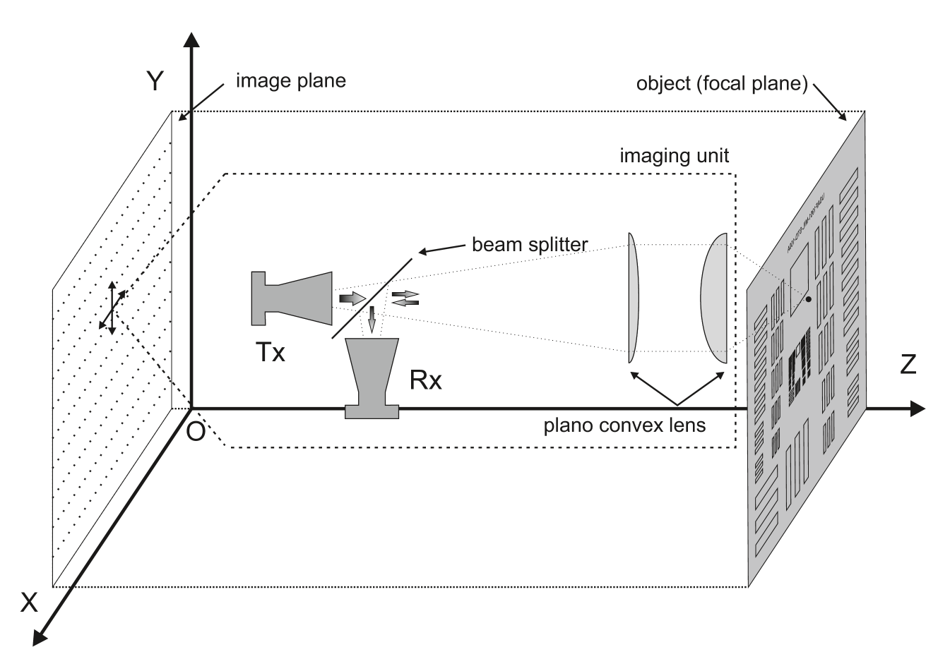
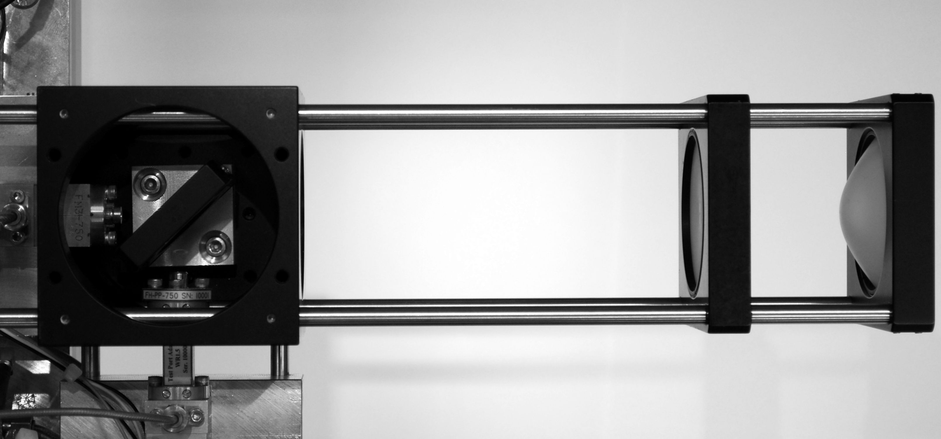
Fig. 1 shows the imaging geometry. Both transmitter (Tx) and receiver (Rx) are mounted on the same platform. The imaging unit, consisting of Tx, Rx and optical components, are moved along the x and y direction using stepper motors and linear stages. This imaging unit takes a depth profile of the object at each lateral position, in order to acquire a full 3D image. The data is acquired with a lateral step size of in xy-direction. During measurement, the motor controller and the data acquisition are synchronized to enable on the fly measurements. An adequate integration time and velocity is chosen in order to provide enough time for the acquisition of 1400 samples per depth profile and 36 averages per sample. The total acquisition time for such an averaged depth profile is ms.
Transmitter (Tx) and receiver (Rx) are mounted in a monostatic geometry. A beam splitter and two hyperbolic lenses focus the beam radiated from the Tx and reflected from the sample into the Rx. By measuring minimum dimension which obtains more than 3dB intensity difference, the resolution of the setup is measured as using a metallic USAF 1951 Resolving Power Test Target scaled to the THz frequency range, which is close to the theoretical ideal expectation of (numerical aperture NA @ GHz). Due to the monostatic scanning approach no optical magnification occurs. The system’s depth resolution is defined by
| (1) |
where is the speed of light in air, and is the system bandwidth. For our system, we have
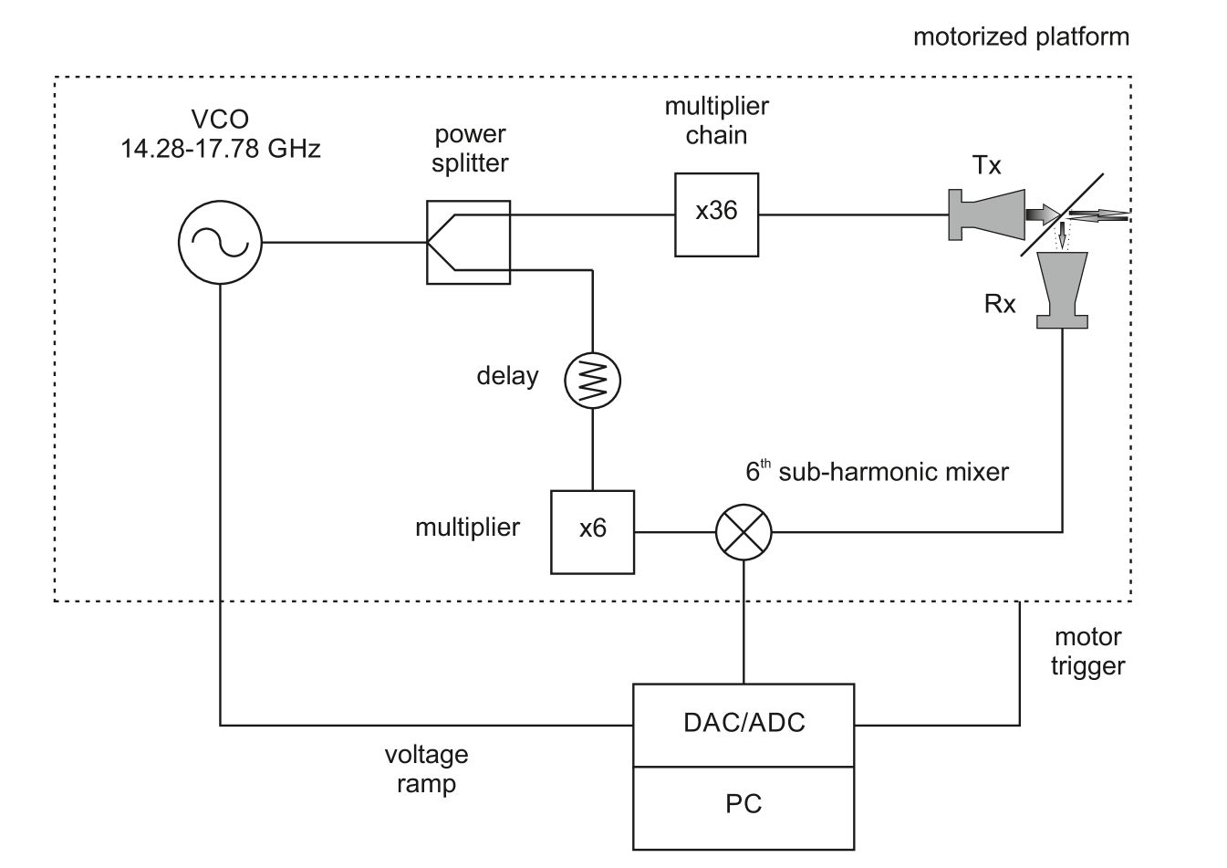
For the FMCW operation, a voltage controlled oscillator (VCO) is tuned from GHz (see Fig. 2). The signal at the output of the VCO is distributed to the Tx and the Rx using a power-splitter. For transmission the signal is then upconverted to GHz with a chain of multipliers. After downconversion to the intermediate frequency (IF) range using a sub-harmonic mixer, which is fed with the 6th harmonic of the VCO signal, the signal is digitized with 10 MS (mega-samples) per second sampling rate and transferred to the host PC. An additional delay between the Tx and Rx path creates a frequency offset in the intermediate frequency signal for proper data acquisition.
4 Proposed method
4.1 Overview
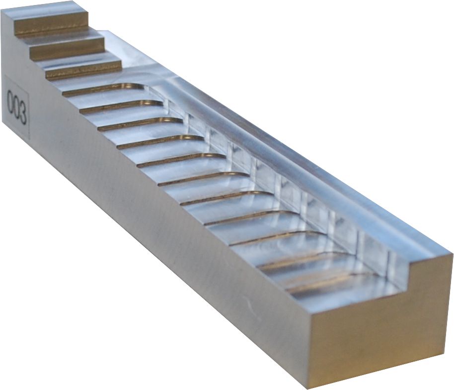
In the previous THz 3D imaging system [7], the signal was assumed to have an ideal flat target with perfect orthogonal alignment to the THz sensor. However, perfect planarity and orthogonality require a high precision of the manufacturing procedure and calibration of the acquisition setup. To study more realistic THz imaging scenarios, we allow for non-planar targets (see Figs. 3 and 5), which are not perfectly orthogonally aligned to the sensor, i.e. that the distance between sensor to a lateral pixel in xy-direction is an unknown variable.
Fig. 4 depicts our method, which comprises three major components: pre-processing, parameter extraction and deconvolution. In the pre-processing part, the measured complex signal is interpolated by zero-padding to obtain more sampling points in -direction. In the parameter extraction part, a complex model is fitted to the in-phase and quadrature components of the signal in z-direction for each lateral position. From this fitting, we deduce corrected reflectance complex field signal and depth information. In the deconvolution part, we process the reconstructed 2D image with deconvolution algorithm to form a high resolution image in xy-domain.
4.2 Preprocessing
With the initial input data to our computational procedure, we have a complex THz signal acquired per-pixel with frequency ramping [29]. In this paper, is denoted as the measured complex signal at lateral position with discrete frequency parameter with length .
In order to achieve sub-wavelength geometric correction, more sampling points on the z-axis are required for robust curve fitting. Based on the current acquisition system (see Sec. 3), an intuitive method is to interpolate the signal in the spatial domain, but the time domain signal provides another option. Instead of spatial interpolation, we extend the discrete signal by a factor of using zero-padding of the complex electric field signal in the frequency domain:
| (2) |
where is the zero-padding factor, and the length of is . In this paper, we use .
After zero-padding, the signal is transformed into the spatial domain by applying a deramp-FFT [29].
| (3) |
The resulting 3D image can be expressed as a 3D matrix in the spatial xyz-domain, representing per-pixel the complex reflectivity of THz energy in z-direction represented by the complex samples .
5 Parameter extraction
In this part, we apply per-pixel parameter extraction in z-direction in order to represent the measured complex signal by a complex reflection model. As each pixel is treated independently, we simplify notation by dropping the pixel-location using, e.g., for .
Our FMCW-THz 3D imaging system is calibrated by amplitude normalization with respect to an ideal metallic reflector. Thus, we achieve an ideal rectangular frequency amplitude signal response, which, after being Fourier transformed, results in an ideal function as continuous spatial signal amplitude. In this model, we assume single layer reflection, and the extension to multi-layer reflection is part of future work. As we assume a single layer reflection, the complex signal model is modeled as a modulated function:
| (4) |
In Eq. (4), is the electric field amplitude, and are the mean (i.e. the depth) and the width of the function, respectively, is the angular frequency of the sinusoidal carrier and is the depth-related phase shift. We formulate the parameter extraction as a complex curve fitting process with respect to optimizing and minimizing the energy function
| (5) |
where the subscripts and denote the real and the imaginary part of a complex number, respectively, and is the fitting window (see Sec. 5.1).
Because of the highly non-linear optimization involved in the curve fitting process, a direct application of Eq. (5) to a non-linear solver potentially results in local minima and does not lead to robust results. Therefore, we apply the following optimization steps which achieve a robust complex curve fitting:
-
1.
Estimate the signal’s maximum magnitude z-position in order to localize the curve fitting window (see Sec. 5.1).
-
2.
Apply a curve fitting to the magnitude signal leading to initial values for (see Sec. 5.2).
-
3.
Estimate the initial phase value using a phase matching with respect to the angle of complex signal (see Sec. 5.3).
- 4.
-
5.
Reconstruct an intensity image and an depth image based on the curve fitting result (sec Sec. 5.4).
Our curve fitting approach significantly reduces the per-pixel intensity inhomogeneity (see Sec. 7.2.2). The subsequent lateral deconvolution algorithm discussed in Sec. 6 involves the numerical solution of an ill-posed inverse problem of finding the blur kernel and enhancing the image’s sharpness at the same time, which is very sensitive to noise. Therefore, correcting the intensity yields two advantages, i.e., it stabilizes the numerical deconvolution process and it prevents wrong interpretations of intensity variation as structural or material transitions. We will provide comparison in Fig. 13 and discuss the lateral resolution enhancement with and without the per-pixel parameter extraction in Sec. 7.3.1.
5.1 Curve Fitting Window
As we focus on the primary reflection signal, assuming that the geometric reflection energy concentrates on the first air-material interface, we locate the z-position that exhibits the maximum magnitude within a fitting window
| (6) |
with center
| (7) |
i.e., is the maximum magnitude z-position in the complex spatial domain data. is the half-width of the fitting window. The choice of is discussed in Sec. 7.1.
5.2 Magnitude Curve Fitting
Since the complex model in Eq. (4) is non-linear and the optimization for in Eq. (5) is non-convex, the estimation of the initial parameters is critical in order to avoid local minima. A reliable initial estimate of the complex curve fitting parameters is deduced from a magnitude curve fitting.
The magnitude signal model is derived from Eq. (4) and is expressed as
| (8) |
where is the electric field amplitude based on signal magnitude, is the center of function, and is the width. The magnitude curve fitting minimizes the energy function by the Trust-Region Algorithm [30]
| (9) |
After the magnitude curve fitting, are the initial values for with respect to the complex signal model in Eq. (4). However, an estimate for the phase angle is still required.
5.3 Estimating the Initial Phase Value
We assume that, within the fitting window , the phase angle in our model (see Eq. (4)) matches the phase angle in the spatial domain data . The corresponding optimization energy functional measures the linear deviation between these phase angles as follows
| (10) |
Setting the gradient of to zero and applying trigonometric identities, we obtain
| (11) |
In Eq. (11), the initial phase angle is independent from the data angle . Therefore, the minimum to Eq. (10) is found by solving for in Eq. (11), yielding
| (12) |
After this phase initialization, and are given as initial values for and in the model in Eq. (4), respectively, and the model is fitted according to the energy function in Eq. (5) using the Trust Region Algorithm [30].
After the complex curve fitting, the four different parameters of our model in Eq. (4) are extracted: amplitude , mean , width , and phase . Because of scattering and multi-layer reflection, error exists if we fit in an ideal sinc-function. Therefore, is extracted as a varying parameter to indicate the error. The depth parameter is evalauted in Sec. 7.2. The amplitude parameter is further processed in a 2D approach. The processing method on all other parameters (, , ) will be investigated in future research.
5.4 Intensity Image Reconstruction
Next, we have to extract the per-pixel intensities using our model. We, therefore, first define the reference intensity image based on the input data as the intensity of the z-slice with the maximum average magnitude:
| (13) |
where is the complex conjugate of and are the size of the matrix in x-axis and y-axis, respectively. The reconstructed intensity is deduced from the curve fitted data model and is defined as the intensity of the model’s signal (Eq. (4)) at the center position :
| (14) |
6 Deconvolution
After the curve fitting, the reconstructed intensity is a 2D image with real and positive values. We can now apply a state-of-art 2D deconvolution algorithm to enhance the xy-domain resolution. In contrast to prior work we use a total variation (TV) blind deconvolution algorithm to improve the spatial resolution [31, 32].
In deconvolution image model, our reconstructed intensity image can be expressed as a blurred observation of a sharp image
| (15) |
where is the spatially invariant point spread function (PSF) (also known as blur kernel) and is the noise; denotes convolution. Blind deconvolution methods allow for estimating the blur kernel directly from the data, which is, however, an ill-posed inverse problem that requires a prior knowledge in order to deduce a robust result [33]. In this paper, we utilize the sparse nature of intensity gradients [34] and choose a state-of-art TV blind deconvolution algorithm that minimizes
| (16) |
Here, is commonly referred as a data term, is a regularization parameter and is the TV-regularization (or prior) that enforces the gradient of the resulting deblurred image to be sparse. As by-product, the blind deconvolution yields the estimated PSF . We obtain our final results using the implementation from Xu et al. [31, 32].
7 Evaluation
In this section we evaluate our image enhancement approach using the following two datasets
-
1.
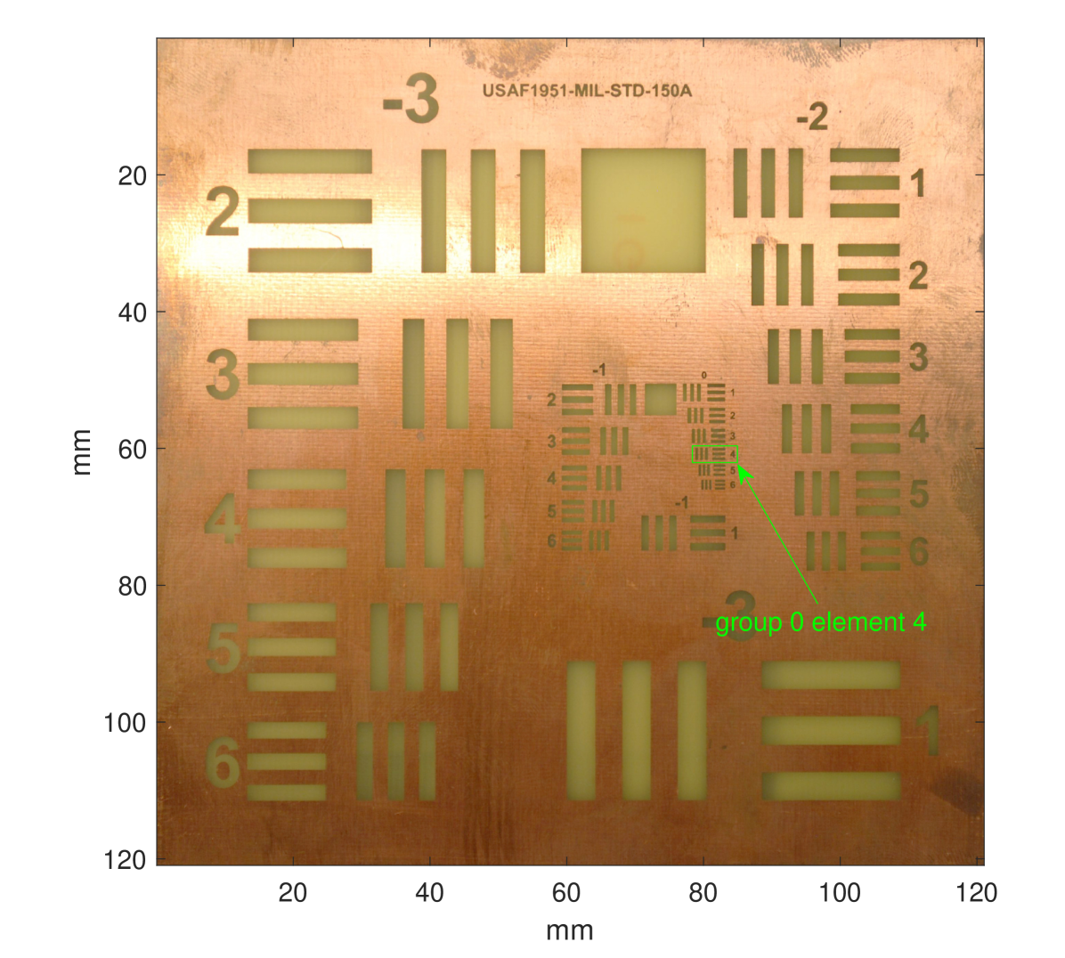
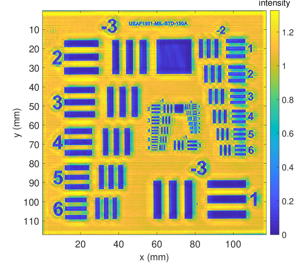
MetalPCB: A nearly planar “USAF” target etched on a circuit board (Fig. 3). The dataset has been acquired using the setup described in Sec. 3 and has the resolution , , . The lateral per-pixel distance (i.e. the sensor mechanical movement distance) is . The target is etched in the standard size scale of USAF target MIL-STD-150A.
- 2.
It should be noted, that our system has a lateral resolution of as its ideal diffraction limit, an experimentally measured lateral resolution and a depth accuracy of as its diffraction limits (see Sec. 3).
We apply and compare the following images, reconstruction and image enhancement methods. The images are named as , where is the intensity image applying deconvolution methods, is the method applied to the intensity image, and is the deblur kernel adopted in the deconvolution method.
-
1.
Refer: The reference intensity image ; no reconstruction using curve fitting and no image enhancement applied.
-
2.
Reconst: The reconstructed intensity image using curve fitting; no image enhancement applied.
- 3.
- 4.
- 5.
- 6.
- 7.
- 8.
In the following, we will first deduce the optimal window size for the quality control of the fitting using the MetalPCB dataset (Sec. 7.1). In Sec. 7.2, we will discuss the depth accuracy using the StepChart dataset. In Sec. 7.3, we will discuss the lateral resolution on MetalPCB dataset. All intensity images are normalized to a perfect metal reflection, and displayed using MATLAB’s perceptionally uniform colormap parula [35].
7.1 Window Size Optimization
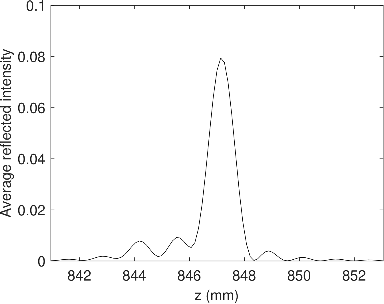
In Fig. 6, the average intensity of by the z-axis in the PCB region of the MetalPCB dataset is shown. We can observe that, compared to the symmetric model in Eq. (4), the z-axis signal has a lower main lobe to side lobe ratio in the PCB region. This might be due to the superposition of signal reflection from the front and back PCB surfaces (see Fig. 3). This indicates that a large fitting window size in Eq. (6) would corrupt any quantitative evaluation and should be avoided. On the other hand, a small fitting window size is also not feasible, as we need a sufficient number of sampling points to get a robust fitting result and to avoid over-fitting.
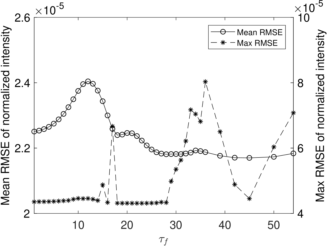
To obtain a reliable numeric measurement, we evaluate the fitting error for varying fitting window half-widths using the Root-Mean-Square-Error (RMSE) between the fitted model (see Eq. (4)) and the spatial data :
| (17) |
As a measure for the full THz image, we calculate the mean and the maximum RMSE over all pixels
| (18) |
In Fig 7, the mean and the maximum RMSE of the curve fitting with a different fitting window are shown. We can see that the mean RMSE and maximum RMSE are both increasing when , which is expected due to over-fitting. When the fitting window is increased to a larger value, we can observe that the mean RMSE is decreased steadily until . The maximum RMSE, however, has no clear tendency and strongly varies beyond . After considering that the mean and maximum RMSE are both considerably low when the window size is 45, we choose as our reference and optimal window size, which is used throughout the rest of the evaluation.
7.2 Depth Accuracy and Intensity Reconstruction
In this section, we analyzed the depth accuracy enhancement in the z-direction obtained by the proposed curve fitting method. In Sec. 7.2.1, the depth accuracy of the StepChart dataset using the maximum magnitude method and the proposed method are shown. In Sec. 7.2.2, we analyze the variance of a homogeneous metal cross section on the MetalPCB dataset.
7.2.1 Depth Accuracy
| Depth Difference | Relative Error | |||||
|---|---|---|---|---|---|---|
| mean | SD | mean | SD | |||
| () | () | () | () | () | () | () |
| 4009.0 | 3898.5 | 7.2 | 3831.3 | 12.4 | 2.76 | 4.43 |
| 2987.0 | 2797.2 | 54.0 | 2810.8 | 13.0 | 6.35 | 5.90 |
| 2006.0 | 1908.7 | 53.6 | 1926.8 | 19.4 | 4.85 | 3.95 |
| 1004.0 | 941.1 | 0.0 | 958.6 | 23.4 | 6.26 | 4.53 |
| 903.0 | 806.7 | 0.0 | 815.3 | 17.5 | 10.67 | 9.71 |
| 803.0 | 792.8 | 40.9 | 742.0 | 14.0 | 1.27 | 7.60 |
| 703.0 | 633.8 | 77.3 | 665.5 | 20.5 | 9.84 | 5.33 |
| 600.0 | 590.0 | 65.6 | 561.9 | 19.5 | 1.66 | 6.35 |
| 472.0 | 403.3 | 0.0 | 468.8 | 13.9 | 14.55 | 0.68 |
| 410.0 | 403.3 | 0.0 | 391.0 | 13.7 | 1.63 | 4.64 |
| 298.0 | 268.9 | 0.0 | 287.6 | 14.7 | 9.77 | 3.48 |
| 208.0 | 268.9 | 0.0 | 192.2 | 15.1 | -29.27 | 7.60 |
| 91.0 | 17.7 | 45.5 | 89.3 | 17.4 | 80.58 | 1.88 |
| 42.0 | 102.2 | 61.8 | 34.9 | 21.9 | -143.28 | 16.84 |
In this part, we evaluate the depth accuracy using the StepChart dataset. In comparison to the depth of the proposed method , we obtain the depth using the maximum magnitude position (Eq.(7)) of .
The z-positions are both calibrated to by the reference zero z-position
| (19) |
where is the zero-padding factor in Eq.(2), is the physical depth per sample, i.e. the systems depth resolution (see Eq. (1)).
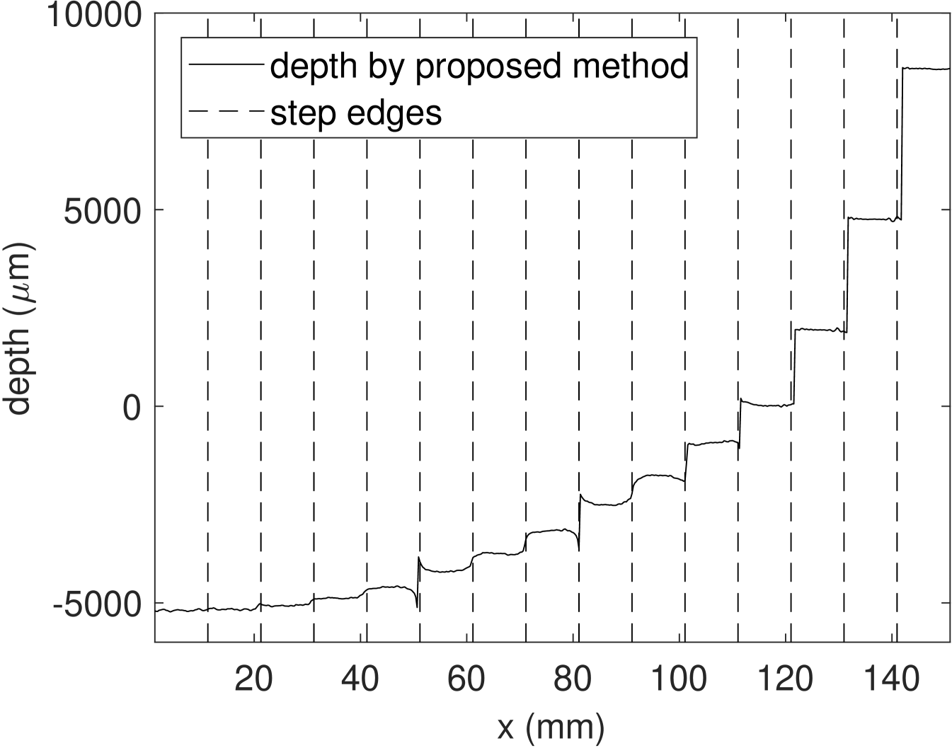
Fig. 8, the cross section depth of StepChart dataset is plotted with an expected position of the edges. We can observe an interference effect due to signal superposition at several edges, most notably at mm and mm. Even though blind deconvolution can hardly resolve strong interference effects, spatially varying point-spread-function is required in order to cope with these kind of effects in the deconvolution stage; see also Hunsche et al. [36].
In order to circumvent interference effects, we extract and average depth values from the center 350 samples for each step. Then, we calculate the depth differences between adjacent steps. These depth differences are compared to the ground truth values, which is obtained by mechanical measurement. Tab. 1 depicts the depth differences and the corresponding standard deviation (SD) of the ground truth , the maximum magnitude method and the proposed curve fitting (see Eq. (19)). In order to compare the depth accuracy, we calculate the relative error as
| (20) |
In this paper, we consider a depth difference as resolvable when the relative error is below with a reasonably low deviation. Thus, our proposed method can still resolve the depth difference, while the maximum magnitude method can only resolve depth difference up to . As a result, the proposed curve fitting method enhances the system depth accuracy to .
7.2.2 Intensity Reconstruction
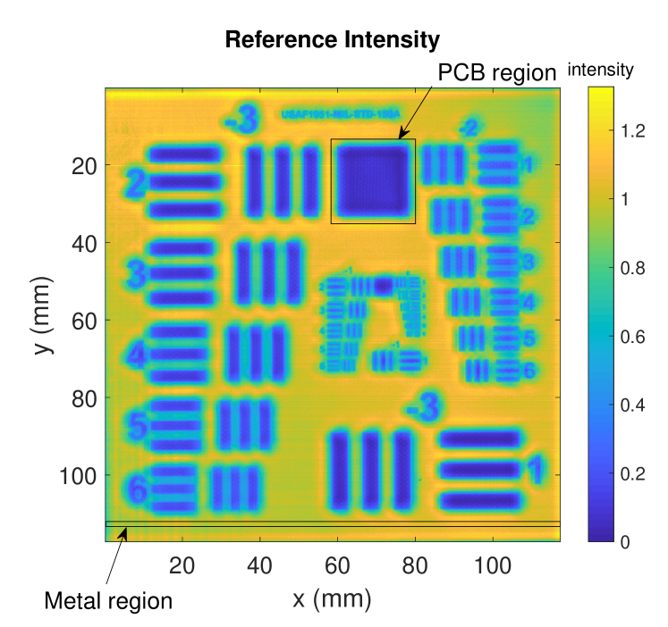
In this part we evaluate the reconstructed intensity image that is directly deduced from our enhanced depth accuracy according to Eq. (14). We, therefore, use the MetalPCB dataset that comprises large homogeneous copper regions. The MetalPCB target is, however, not perfectly flat and/or not perfectly aligned orthogonally.
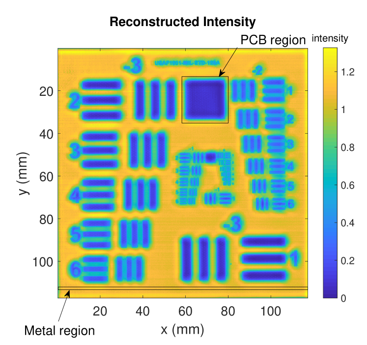
Fig. 9 depicts the intensity images for the reference intensity based on Eq. (13) (Fig. 9a) and the proposed reconstructed intensity using Eq. (14) (Fig. 9b). We can observe that the copper regions do not appear to be fully homogeneous in reference intensity image . After applying the high accuracy depth reconstruction, this intensity inhomogeneity is significantly reduced in the reconstructed image .
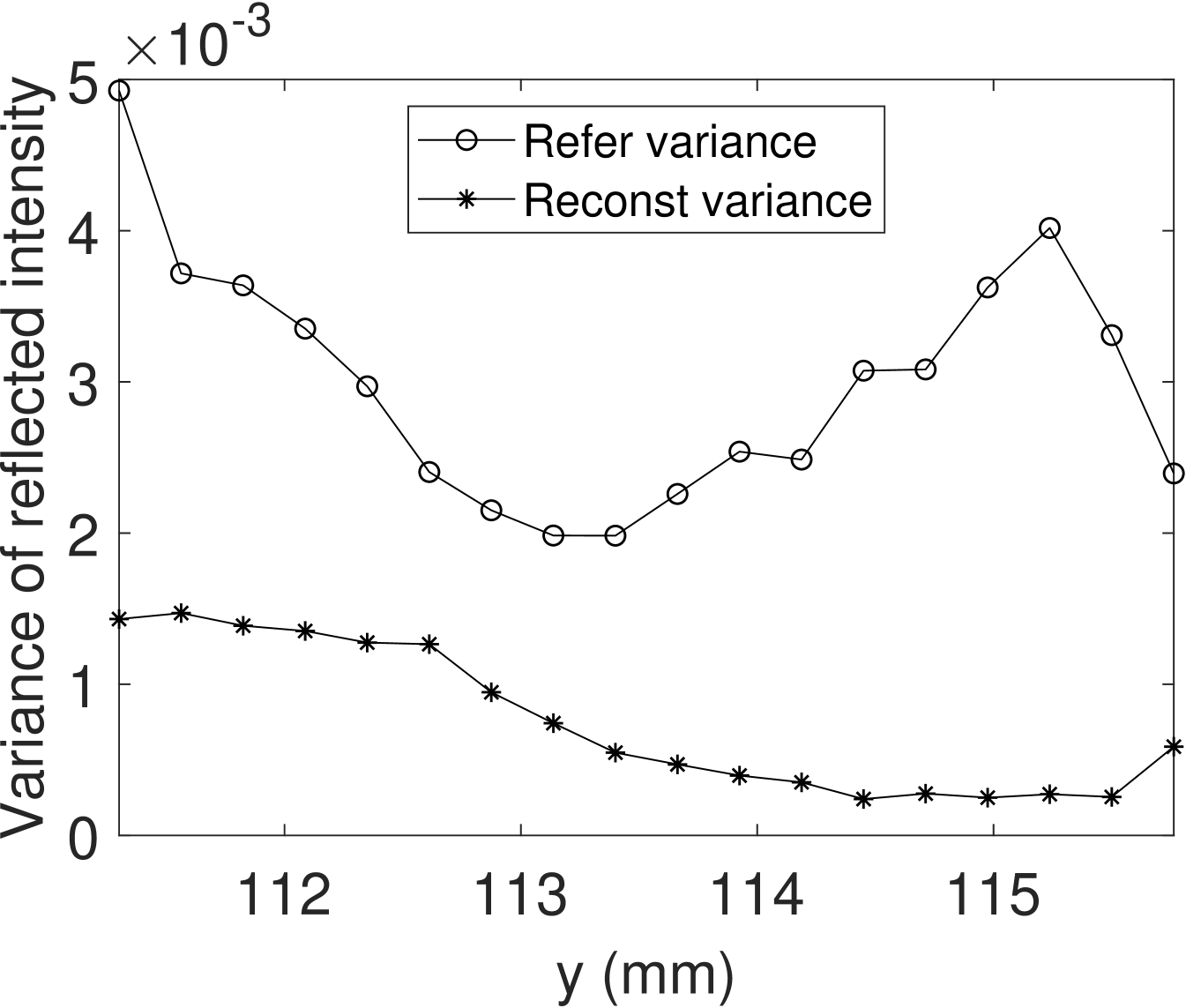
Fig. 10 further analyzes the intensity homogeneity using a horizontal metal region (see Fig. 9, lower image part). The horizontal metal region consists of 18 pixel rows for each of which we compute the intensity variance in the reference intensity image and the reconstructed intensity image . We observe that the reconstruct intensity has a significantly reduced intensity variance within all rows of copper, as the reconstruct intensity is focused on an accurate depth position for each lateral position.
7.3 Lateral Resolution and Analysis
In this section, we analyzed the lateral domain enhancement by the proposed method using the MetalPCB dataset. In Sec. 7.3.1, we compared the proposed method to Lucy-Richardson’s deconvolution method on behalf of the lateral resolution and in Sec. 7.3.2 we visually analyze the silk structure embedded in the PCB region.
7.3.1 Lateral resolution

| Method | Figure |
|
|
|
|
||||||||||||
|---|---|---|---|---|---|---|---|---|---|---|---|---|---|---|---|---|---|
| Reconst() | Fig. 9b | 794.3 | – | 762.0 | – | ||||||||||||
| Reconst_LR-G | Fig. 13b | 419.4 | 1.89 | 393.3 | 1.94 | ||||||||||||
| Reconst_LR-Xu | Fig. 13d | 402.3 | 1.97 | 368.6 | 2.07 | ||||||||||||
| Reconst_Xu()1 | Fig. 13f | 346.2 | 2.29 | 359.6 | 2.12 | ||||||||||||
| 1 Reconst_Xu is the proposed method, | |||||||||||||||||
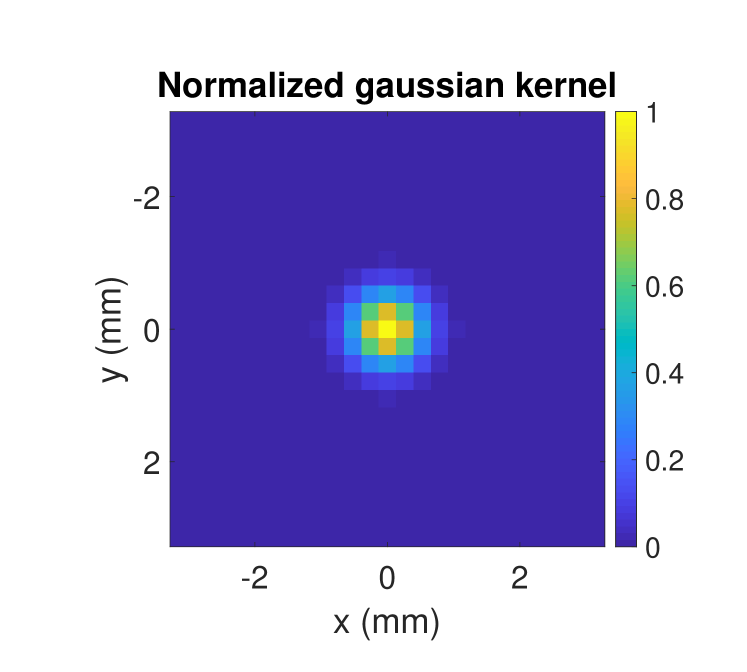
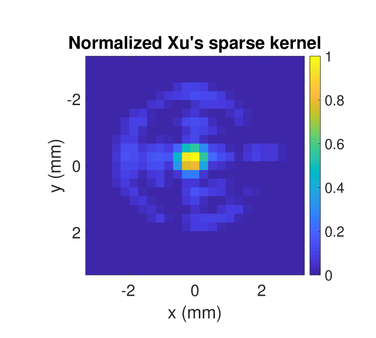
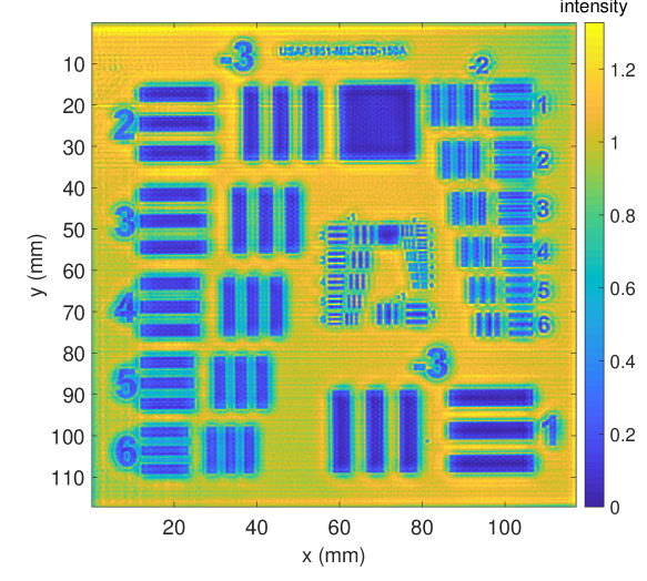
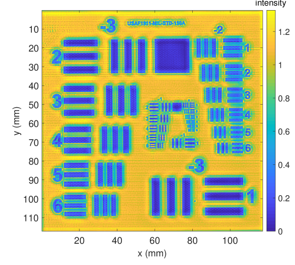
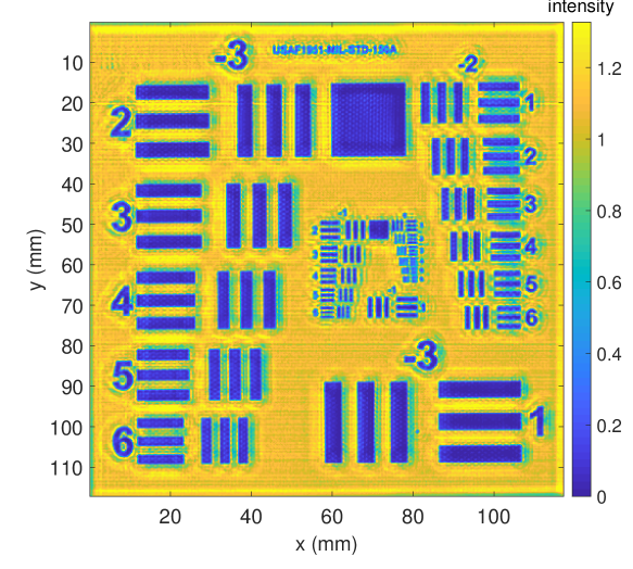
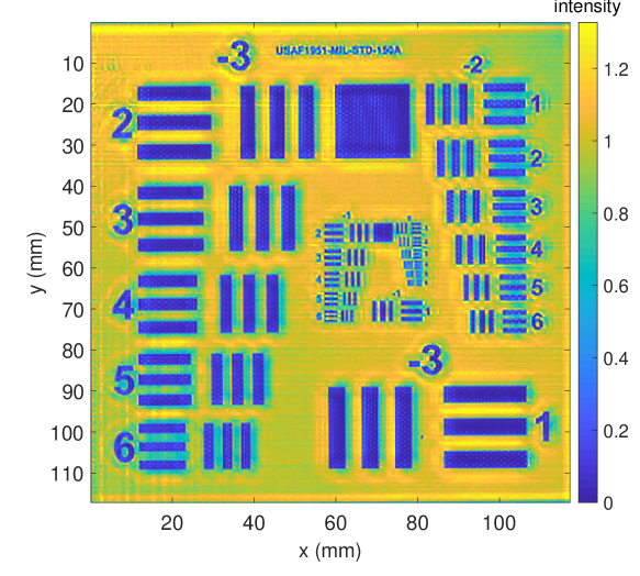
In Fig. 13, we show different output intensity images with respect to the input intensity image, the deconvolution method and the blur kernel. The left column shows the deconvolution results based on the reference intensity image , whereas the right column depicts the results using the reconstructed intensity image . For deconvolution, we apply Xu et al.’s method [31, 32] (Refer_Xu, Reconst_Xu, top row) and Lucy-Richardson’s original method using a gaussian kernel based on the theoretical numeric aperture (Fig. 12a) (Refer_LR-G, Reconst_LR-G, center row), because the Lucy-Richardson’s deconvolution method with a gaussian kernel based on the system numerical aperture is a commonly applied THz deblurring method [12] [13] [14]. We, furthermore, extract the sparse kernel estimated by Xu et al.’s method (Fig. 12b) and plug it into the Lucy-Richardson approach (Refer_LR-Xu, Reconst_LR-Xu, bottom row). Note, that Reconst_Xu (Fig. 13f), is equal to , the method proposed in this paper.
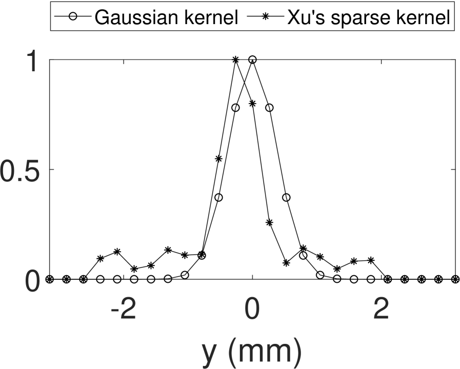
In Fig. 12a and Fig. 12b, the gaussian kernel and Xu’s sparse kernel computed by blind deconvolution are shown respectively. Obviously, the kernel estimated by Xu’s method models further effects related to the imaging system and/or the observed target that are not covered by the gaussian kernel; we will investigate these influences in our future work. In Fig. 12c, we can observe that Xu’s sparse kernel is not centered in the y-axis. This is because the blind deconvolution does not assume any symmetric and centralized property during kernel optimization, but instead the kernel weights are optimized as fully independent parameters throughout the process.
Comparing the results visually, we clearly see that Refer_LR-G, Reconst_LR-G (Lucy-Richardson with gaussian kernel), which has previously been used for THz resolution enhancement (see Sec. 2), yields inferior results in terms of sharpness and local contrast. Xu et al.’s method that estimates the blur kernel from the given intensity image yields much sharper images with improved local contrast (Refer_Xu, Reconst_Xu). Using Xu et al.’s kernel instead of the standard gaussian kernel clearly improves the results obtained by Lucy-Richardson (Refer_LR-Xu, Reconst_LR-Xu). On the downside, Xu et al.’s and Lucy-Richardson’s method with Xu’s kernel increase noise and overshooting effects. Xu et al.’ result is, however, less affected by these artefacts. Apparently, all three methods benefit from the enhanced intensity image using our reconstruction method.
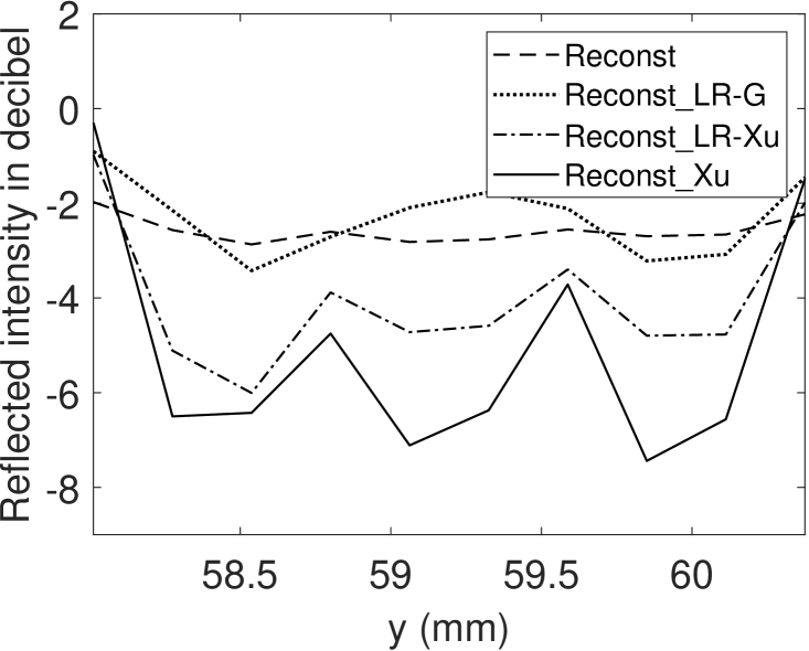
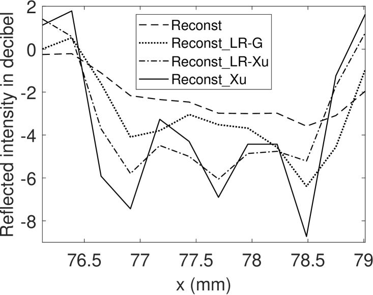
Moreover, Fig. 11 depicts the resolution enhancement using a cross section of group 0 element 4 of the USAF test target (see Fig. 3), representing a line distance of . The cross section intensities before deconvolution (Reconst) and after deconvolution (Reconst_LR-G, Reconst_Xu, Reconst_LR-Xu) are shown respectively (refer to Fig. 9b, 13b, 13f and 13d). Only the proposed method Reconst_Xu can resolve this resolution according to the criterion. One should note that there are different definitions for resolution as discussed in [37]. However, the center position of Reconst_LR-Xu, Reconst_Xu are both shifted, because the sparse kernel Fig. 12b is not centered at the middle. Although blind deconvolution does not retain the absolute intensity position, relative intensity positions are constant because we assume a spatial invariant blur kernel.
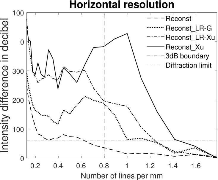
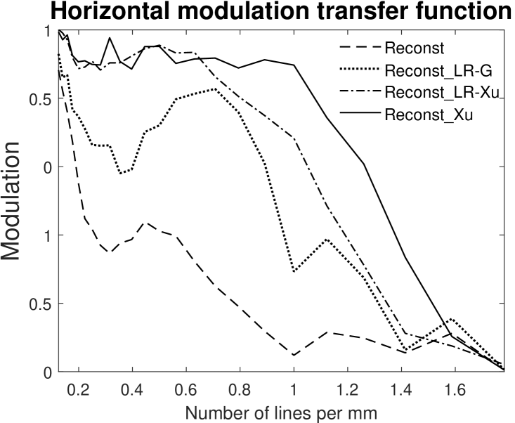
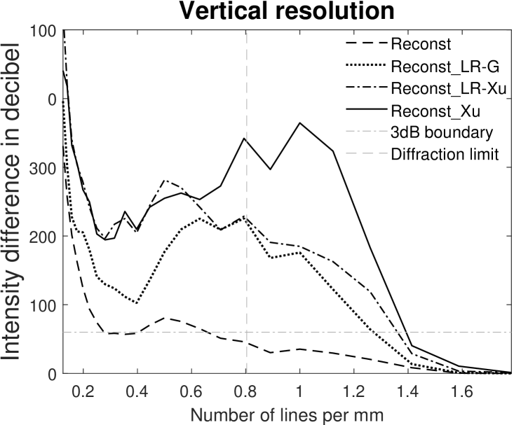
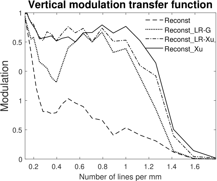
In order to quantify a lateral resolution, we evaluate the contrast at each of the horizontal and vertical resolution patterns of the MetalPCB dataset (USAF target). In case of vertical stripes, we determine the minimal and maximal intensity values for each row crossing the pattern’s edges given its known geometric structure. After removing 10% of the cross sections in the boundary area, the mean value is computed as intensity difference (in ). Analogously, we compute the intensity difference for the horizontal stripes. Fig. 14 shows the intensity difference by the number of lines per mm and the modulation transfer function (MTF) [38, 39] for all methods for vertical and horizontal resolutions. Commonly, to avoid simple enhancement by linear multiplication, a logarithmic measurement over intensity difference is considered as resolution boundary. Tab. 2 depicts the highest resolution at which each method delivers . We notice, that there is a resolution improvement from the non-deconvoluted image (Reconst), via the original Lucy-Richardson method (Reconst_LR-G) and the one using Xu’s kernel (Reconst_LR-Xu), finally, to the proposed method (Reconst_Xu). Taking the limit as boundary, we find horizontal improvement factors (in terms of resolution) of for the proposed method Reconst_Xu and of and for the Lucy-Richardson Reconst_LR-G and the improved Lucy-Richardson Reconst_LR-Xu, respectively. For the vertical resolution, the proposed method has a vertical improvement factor of , while the Lucy-Richardson methods and the improved Lucy-Richardson method have vertical improvement factor , respectively. With respect to the modulation transfer function, Fig. 14b and Fig. 14d show a significantly higher contrast for the proposed method (Reconst_Xu) compared to both, the Lucy-Richardson (Reconst_LR-G) and improved Lucy-Richardson (Reconst_LR-Xu) method.
7.3.2 Embedded Structures
In this part, we analyzed the PCB region on MetalPCB dataset more closely in order to investigate the effect of our enhanced lateral resolution on the embedded silk structures.
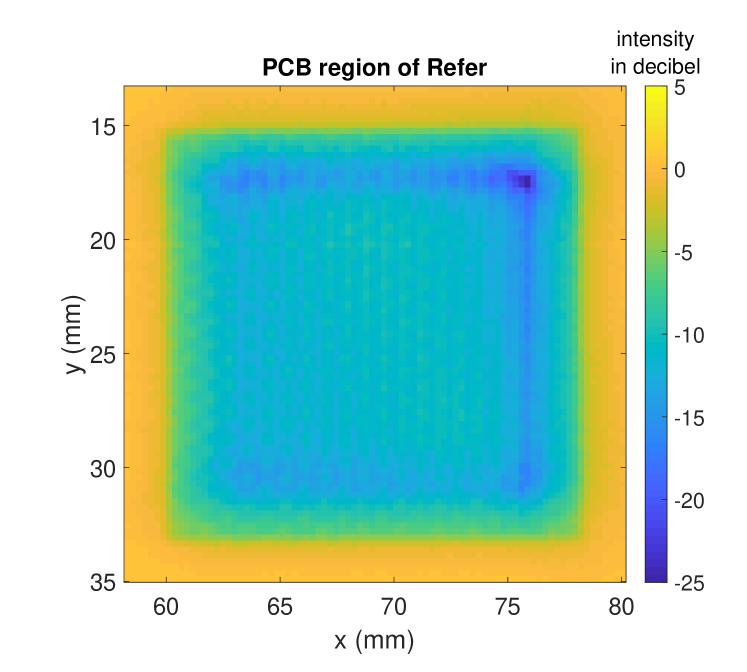
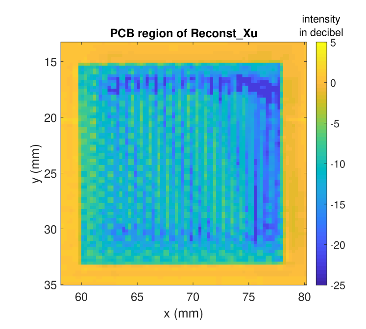
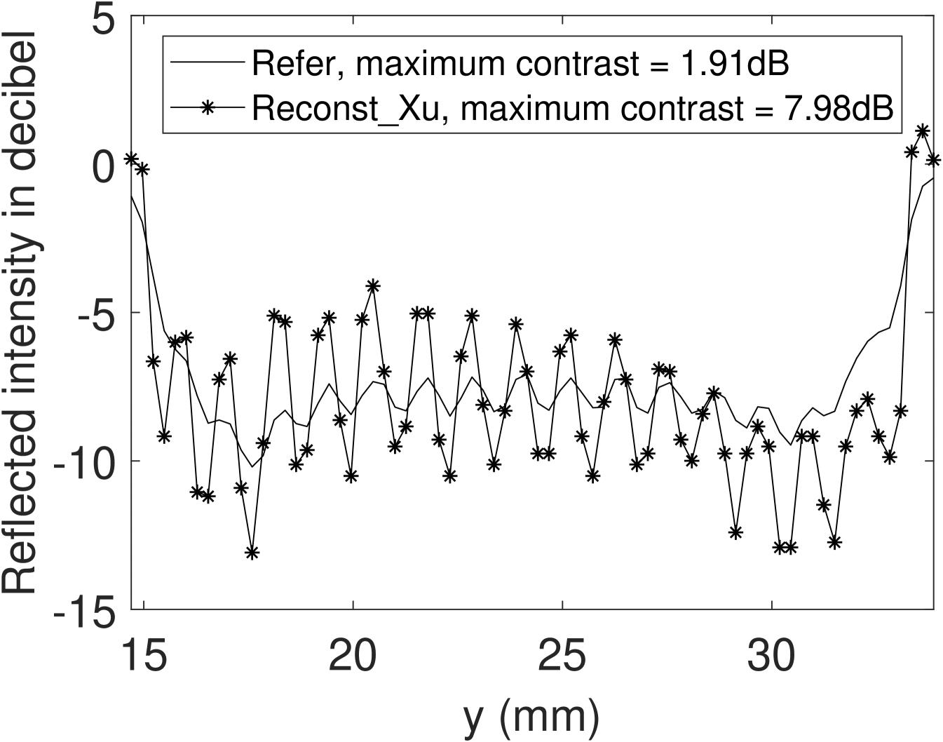
In Fig. 15, the PCB region of the reference intensity Refer (see Fig. 9a) and the proposed deconvoluted intensity Reconst_Xu (see Fig. 13f) are shown. We can observe that a periodic intensity pattern is visible by the enhanced lateral resolution that is caused by woven silk material embedded in the PCB region. The silk fibers introduce a second energy reflection to the imaging system. In Fig. 16, the cross section intensity of the PCB regions in decibel scale are shown. Extracting the maximum contrast within the PCB region we find an enhancement from to . Even though the proposed method nicely emphasizes the periodic silk structure underneath the polymer surface material, we cannot extract the depth of this embedded structure with our approach, as the handling of multi-reflection effects is beyond the scope of this paper. Multi-reflection effects are part of the future work.
8 Conclusion
In this paper, we propose a THz computational image enhancement method to enhance the lateral resolution and depth accuracy beyond the diffraction limit. The method is based on a complex curve fitting on THz 3D image azimuth axis, and a blind deconvolution method on the lateral domain. The experiment results show that our curve fitting method enhances the depth accuracy to . Because of this enhanced depth accuracy, the experiment also shows that the proposed reconstruction method achieves improved intensities on homogeneous, non-planar material regions without introducing additional distortions or noise.
Based on the reconstructed intensities, we apply several lateral blind deconvolution methods. Evidently, all three examined THz deconvolution methods benefit from the enhanced intensity image using our method. In comparison to the classical Lucy-Richardson deconvolution algorithm, the experiments show that the proposed blind deconvolution method achieves the best horizontal resolution enhancement from to , yielding an improvement factor of . In terms of intensity contrast, the proposed method clearly outperforms earlier approaches. Moreover, the experiments show that the proposed method is able to emphasize fine silk texture embedded within a polymer material.
Acknowledgement
This research was funded by the German Research Foundation (DFG) as part of the research training group GRK 1564 Imaging New Modalities.
This is a pre-print of an article published in Journal of Infrared, Millimeter, and Terahertz Waves. The final authenticated version is available online at: https://doi.org/10.1007/s10762-019-00609-w
References
- [1] Hu, B.B., Nuss, M.C.: Imaging with terahertz waves. Optics letters 20(16), 1716–1718 (1995)
- [2] Siegel, P.H.: Terahertz technology. IEEE Transactions on microwave theory and techniques 50(3), 910–928 (2002)
- [3] Chan, W.L., Deibel, J., Mittleman, D.M.: Imaging with terahertz radiation. Reports on progress in physics 70(8), 1325 (2007)
- [4] Jansen, C., Wietzke, S., Peters, O., Scheller, M., Vieweg, N., Salhi, M., Krumbholz, N., Jördens, C., Hochrein, T., Koch, M.: Terahertz imaging: applications and perspectives. Appl. Opt. 49(19), E48–E57 (2010)
- [5] Cooper, K.B., Dengler, R.J., Llombart, N., Thomas, B., Chattopadhyay, G., Siegel, P.H.: Thz imaging radar for standoff personnel screening. IEEE Transactions on Terahertz Science and Technology 1(1), 169–182 (2011)
- [6] McClatchey, K., Reiten, M., Cheville, R.: Time resolved synthetic aperture terahertz impulse imaging. Applied physics letters 79(27), 4485–4487 (2001)
- [7] Ding, J., Kahl, M., Loffeld, O., Haring Bolívar, P.: Thz 3-d image formation using sar techniques: simulation, processing and experimental results. IEEE Transactions on Terahertz Science and Technology 3(5), 606–616 (2013)
- [8] Kahl, M., Keil, A., Peuser, J., Löffler, T., Pätzold, M., Kolb, A., Sprenger, T., Hils, B., Haring Bolívar, P.: Stand-off real-time synthetic imaging at mm-wave frequencies. In: Passive and Active Millimeter-Wave Imaging XV, vol. 8362, p. 836208 (2012)
- [9] Ahi, K., Asadizanjani, N., Shahbazmohamadi, S., Tehranipoor, M., Anwar, M.: Terahertz characterization of electronic components and comparison of terahertz imaging with x-ray imaging techniques 9483 (2015)
- [10] Johnson, J.L., Dorney, T.D., Mittleman, D.M.: Interferometric imaging with terahertz pulses. IEEE Journal of selected topics in quantum electronics 7(4), 592–599 (2001)
- [11] Chen, H.T., Kersting, R., Cho, G.C.: Terahertz imaging with nanometer resolution. Applied Physics Letters 83(15), 3009–3011 (2003)
- [12] Xu, L.M., Fan, W.H., Liu, J.: High-resolution reconstruction for terahertz imaging. Applied optics 53(33), 7891–7897 (2014)
- [13] Li, Y., Li, L., Hellicar, A., Guo, Y.J.: Super-resolution reconstruction of terahertz images. In: SPIE Defense and Security Symposium, pp. 69490J–69490J. International Society for Optics and Photonics (2008)
- [14] Ding, S.H., Li, Q., Yao, R., Wang, Q.: High-resolution terahertz reflective imaging and image restoration. Applied optics 49(36), 6834–6839 (2010)
- [15] Hou, L., Lou, X., Yan, Z., Liu, H., Shi, W.: Enhancing terahertz image quality by finite impulse response digital filter. In: Infrared, Millimeter, and Terahertz waves (IRMMW-THz), 2014 39th International Conference on, pp. 1–2. IEEE (2014)
- [16] Ahi, K., Anwar, M.: Developing terahertz imaging equation and enhancement of the resolution of terahertz images using deconvolution. In: SPIE Commercial+ Scientific Sensing and Imaging, pp. 98560N–98560N. International Society for Optics and Photonics (2016)
- [17] Walker, G.C., Bowen, J.W., Labaune, J., Jackson, J.B., Hadjiloucas, S., Roberts, J., Mourou, G., Menu, M.: Terahertz deconvolution. Optics express 20(25), 27230–27241 (2012)
- [18] Chen, Y., Huang, S., Pickwell-MacPherson, E.: Frequency-wavelet domain deconvolution for terahertz reflection imaging and spectroscopy. Optics express 18(2), 1177–1190 (2010)
- [19] Takayanagi, J., Jinno, H., Ichino, S., Suizu, K., Yamashita, M., Ouchi, T., Kasai, S., Ohtake, H., Uchida, H., Nishizawa, N., et al.: High-resolution time-of-flight terahertz tomography using a femtosecond fiber laser. Optics express 17(9), 7533–7539 (2009)
- [20] Lucy, L.B.: An iterative technique for the rectification of observed distributions. The astronomical journal 79, 745 (1974)
- [21] Richardson, W.H.: Bayesian-based iterative method of image restoration. JOSA 62(1), 55–59 (1972)
- [22] Knobloch, P., Schildknecht, C., Kleine-Ostmann, T., Koch, M., Hoffmann, S., Hofmann, M., Rehberg, E., Sperling, M., Donhuijsen, K., Hein, G., et al.: Medical thz imaging: an investigation of histo-pathological samples. Physics in Medicine & Biology 47(21), 3875 (2002)
- [23] Xie, Y.Y., Hu, C.H., Shi, B., Man, Q.: An adaptive super-resolution reconstruction for terahertz image based on mrf model. In: Applied Mechanics and Materials, vol. 373, pp. 541–546. Trans Tech Publ (2013)
- [24] Gu, S., Li, C., Gao, X., Sun, Z., Fang, G.: Three-dimensional image reconstruction of targets under the illumination of terahertz gaussian beam—theory and experiment. IEEE Transactions on Geoscience and Remote Sensing 51(4), 2241–2249 (2013)
- [25] Dong, J., Wu, X., Locquet, A., Citrin, D.S.: Terahertz superresolution stratigraphic characterization of multilayered structures using sparse deconvolution. IEEE Transactions on Terahertz Science and Technology 7(3), 260–267 (2017)
- [26] Sun, Z., Li, C., Gu, S., Fang, G.: Fast three-dimensional image reconstruction of targets under the illumination of terahertz gaussian beams with enhanced phase-shift migration to improve computation efficiency. IEEE Transactions on Terahertz Science and Technology 4(4), 479–489 (2014)
- [27] Liu, W., Li, C., Sun, Z., Zhang, Q., Fang, G.: A fast three-dimensional image reconstruction with large depth of focus under the illumination of terahertz gaussian beams by using wavenumber scaling algorithm. IEEE Transactions on Terahertz Science and Technology 5(6), 967–977 (2015)
- [28] Standard, M.: Photographic lenses (1959). URL http://www.dtic.mil/dtic/tr/fulltext/u2/a345623.pdf
- [29] Munson, D.C., Visentin, R.L.: A signal processing view of strip-mapping synthetic aperture radar. IEEE Transactions on Acoustics, Speech, and Signal Processing 37(12), 2131–2147 (1989)
- [30] Coleman, T.F., Li, Y.: An interior trust region approach for nonlinear minimization subject to bounds. SIAM Journal on optimization 6(2), 418–445 (1996)
- [31] Xu, L., Jia, J.: Two-phase kernel estimation for robust motion deblurring. In: European conference on computer vision, pp. 157–170. Springer (2010)
- [32] Xu, L., Zheng, S., Jia, J.: Unnatural l0 sparse representation for natural image deblurring. In: Proceedings of the IEEE Conference on Computer Vision and Pattern Recognition, pp. 1107–1114 (2013)
- [33] Levin, A., Weiss, Y., Durand, F., Freeman, W.T.: Understanding blind deconvolution algorithms. IEEE transactions on pattern analysis and machine intelligence 33(12), 2354–2367 (2011)
- [34] Perrone, D., Favaro, P.: Total variation blind deconvolution: The devil is in the details. In: Proceedings of the IEEE Conference on Computer Vision and Pattern Recognition, pp. 2909–2916 (2014)
- [35] MathWorks Inc.: Using colormaps (2016). URL https://www.mathworks.com/help/matlab/examples/using-colormaps.html
- [36] Hunsche, S., Koch, M., Brener, I., Nuss, M.: Thz near-field imaging. Optics communications 150(1), 22–26 (1998)
- [37] Forshaw, M., Haskell, A., Miller, P., Stanley, D., Townshend, J.: Spatial resolution of remotely sensed imagery a review paper. International Journal of Remote Sensing 4(3), 497–520 (1983)
- [38] Boreman, G.D.: Modulation transfer function in optical and electro-optical systems, vol. 21. SPIE press Bellingham, WA (2001)
- [39] Smith, W.J.: Modern optical engineering. Tata McGraw-Hill Education (1966)