Computations about formal multiple zeta spaces defined by binary extended double shuffle relations
Abstract
The formal multiple zeta space we consider with a computer is an -vector space generated by formal symbols for a given weight , where the symbols satisfy binary extended double shuffle relations. Up to weight , we compute the dimensions of the formal multiple zeta spaces, and verify the dimension conjecture on original extended double shuffle relations of real multiple zeta values. Our computations adopt Gaussian forward elimination and give information for spaces filtered by depth. We can observe that the dimensions of the depth-graded formal multiple zeta spaces have a Pascal triangle pattern expected by the Hoffman mult-indices.
1 Introduction
The space generated by multiple zeta values (MZVs for short) has been elucidated theoretically and numerically in recent years, but its structure remains mysterious. In this paper, we shed light on a formal space generated by binary analogs of MZVs by computer experiments for unraveling both of the original and formal spaces.
Let denote the set of positive integers. The MZV is a real number that belongs to an image of a function (customarily denoted by ) whose domain is
| (1.1) |
where is the empty mult-index and . We call and the weight and depth, respectively. The function has two definitions by the iterated integral and nested summation, which endow the -vector space spanned by MZVs with abundant linear relations. Euler [13], who solved the Basel problem and advanced the case , also studied the case .
Zagier [34] conjectured111 Zagier noted the conjectures were made after many discussions with Drinfel’d, Kontsevich and Goncharov. that is graded by weight and the dimensions of graded pieces are expressed in terms of a Fibonacci-like sequence. Let be the subset consisting of mult-indices of weight , and let be the subspace spanned by MZVs in . The dimension conjecture is
| (1.2) |
where , and . These integers fit together into the generating series
| (1.3) |
The ultimate upper bound theorem (i.e., ) was established independently by Goncharov [10, 16] and Terasoma [32]. Brown [8] furthermore proved that is generated by MZVs in , where is the set of Hoffman mult-indices of weight :
| (1.4) |
Hoffman [18] conjectured is a basis of , which would imply the dimension conjecture because the same recurrence relation holds by a simple count of the number of ’s and ’s. Umezawa [33] also suggested a basis conjecture in terms of iterated log-sine integrals, in which sets of mult-indices different from are used. Because of the difficulty to show the independence between MZVs, no non-trivial lower bounds are known.
By the upper bound theorem, it is natural to ask that what sorts of relations are needed to reduce the number of generators of to . There are several conjectural candidates: e.g., [11, 14, 17, 22, 23]. In particular, the extended double shuffle (EDS) relations [19, 29] known from early on are often selected for experimentally attacking this question, because they are easier to write down and included in the other candidates except Kawasima’s [23]. Minh and Petitot [28] verified that the class of EDS relations is a right candidate up to weight , Bigotte et al. [5] verified it up to weight , Minh et al. [27] verified it up to weight ,222 This experimental result was announced in their private communication (see [21, Section 1]). Espie et al. [12] verified it up to weight , and Kaneko et al. [21] verified it up to weight that seems to be the latest record. The first two experiments are by the Gröbner basis method, and the last three ones are by the vector space (or matrix) method. The fourth one of [12] was executed under modulo rational multiples of powers of , or module .
The first purpose of this paper is to improve the record to weight . For this, we consider an -vector space instead of the -vector space : roughly speaking, is generated by binary multiple zeta symbols (binary MZSs for short), where satisfy binary EDS relations that are obtained from original EDS relations after the modulo arithmetic to integer coefficients. (Exact definitions of the binary analogs in this section will be stated in the next section.) We will verify is a basis of and . Our calculation results break the record because (as will be mentioned in Section 3). The space reduces the computation cost since is the binary and simplest finite field. The field makes it easy to apply useful techniques in computer since is compatible with the Boolean datatype: in fact, we will employ a conflict based algorithm discussed in [24] for a fast Gaussian forward elimination.
The second and main purpose is to observe a Pascal triangle pattern in from the viewpoint of a direct sum decomposition,
| (1.5) |
where are quotient spaces defined by means of depth filtration: the descending chain is used for , where are the subspaces spanned by binary MZSs of weight and depth at most . We define and
| (1.6) |
with . We denote by the canonical image333 We use the same notation for all canonical images in the quotient spaces . There should be no confusion because the quotient space under consideration is clear from context. of in for any . Up to weight , we will verify is a basis of and . Counting the number of ’s and ’s implies that the double sequence satisfies a recurrence relation with a Pascal triangle pattern: , and for other and , or equivalently,
| (1.7) |
More precisely, since the integers satisfy the same recurrence relation as the binomial coefficients . As expected from (1.5), the formula (1.7) specializes to (1.3) upon .
We also try experiments on parts of EDS relations, ‘’ and ‘’ relations, which are expected to be alternatives to EDS and actually employed in [21, 27] for verification, respectively. Unlike the case in , those relations do not suffice to give all relations in , but we can find a quasi Fibonacci-like rule in dimensions of spaces defined by relations.
The idea of the depth filtration in (1.5) was conceived by Broadhurst and Kreimer [7] to propose a refinement of the dimension conjecture. Their conjecture indicates two interesting facts in the -vector spaces of MZVs graded by both weight and depth: (i) modular forms influence the structure through quotient spaces defined by the -version of (1.5); and (ii) the Hoffman values are irrelevant to the structure in the sense that most of the values vanish in the graded pieces of same depth. In terms of the generating series, the conjecture is
| (1.8) |
where , and , and is the generating series of the dimensions of the vector spaces of cusp forms on the full modular group. Specific examples for are given in [15] and a modern formulation is discussed in [9] (see also [31]). However our computational results suggest the following when we adopt as the scalar field instead of : (i) the influence of modular forms disappears; but (ii) the Hoffman symbols remain as basis elements with a Pascal triangle pattern.
It should be noted that the Broadhurst-Kreimer conjecture has two equivalent formulations of vector and algebra (see [19, Appendix]). The equivalence requires is isomorphic to the polynomial ring in one variable over . The isomorphy does not hold when is the scalar field as will be mentioned in the final section, and we will consider only the vector formulation in this paper.
It should also be noted that Blümlein et al. [6] provided a data mine for not only MZVs but also Euler sums by experiments to Broadhurst-Kreimer type conjectures, in which it was verified that the union of EDS and duality relations suffices to reduce the number of generators of to up to weight : it was also verified up to by using modular arithmetic, and up to and more with an additional conjecture and limited depths. The duality relations, which are obtained by the integral definition of MZVs and a change of variables, are very useful to compute because they can bring down the size of relations by about half. It has not been proved yet that the EDS relations include the duality relations, although the inclusion is expected to be true conjecturally: in other words, we have not succeeded in understanding the duality of MZVs algebraically. The experimental approaches of [6] and ours differ in the use of the duality relations.
The organization of this paper is as follows. In Section 2, we state exact definitions of the binary MZVs , the formal multiple zeta spaces and the quotient spaces . We report our computational results in Section 3, and explain how our computer programs produce the results in Section 4. The programs are available at the open-source site GitHub.444https://github.com/machide-tomoyan/BMZS-calculator Section 5 is devoted to problems about formal multiple zeta spaces which arise from the computational results. In Appendix, we describe an essential algorithm in our experiments, which employs a conflict based search and speeds up the Gaussian forward elimination under certain conditions.
2 Formal multiple zeta space over
The formal multiple zeta space of weight is briefly defined by
| (2.1) |
where are indeterminates. That is, is an -vector space generated by formal symbols that satisfy binary variations of the EDS relations. Eight equivalent statements are given in [19, Theorem 2] for the EDS relations. In this paper, we choice the statement (v) in the theorem because the relations are all -linear and fewer in number.
To define (2.1) exactly, we require the algebraic setup by Hoffman [18] which allows us the steady handling of two products, the shuffle and stuffle : the latter is also called harmonic or quasi-shuffle. Let be the polynomial ring in the two non-commutative variables and . We call each variable a letter, and a monomial in the variables a word. The shuffle product is a -bilinear product on , which satisfies and
| (2.2) |
for any words and letters . Let denote a word for any , and let be the polynomial ring , or equivalently, the subring in . The stuffle product is a -bilinear product on , which satisfies and
| (2.3) |
for any words and integers . By induction on the lengths of words, both products are commutative and associative, and both and are commutative -algebras. We notice is a parent space of . Let , where and . Both and are subalgebras since is closed under and . The pair of spaces satisfies the polynomial ring property in one variable: the former is freely generated by over the latter on each of and . We thus have
| (2.4) |
We introduce the EDS relations stated in [19, Theorem 2(v)]. Let denote a homomorphism from to , which is defined by taking the constant term with respect to in the first isomorphism of (2.4):555 The homomorphism of stuffle type exists as well, but it is intractable because EDS relations of that type are not always -linear: see [19] (or [2, 20]) for details.
| (2.5) |
Let , and let
For any pair of mult-indices in , we define
| (2.6) |
The objective EDS relations of weight are stated as
| (2.7) |
where is the -linear map (or evaluation map) defined by . We have by (2.5)
We can thus divide (2.7) into two parts:
| (2.8) | |||||
| (2.9) |
where . The relations in (2.8) are called the finite double shuffle (FDS) relations, because MZVs are defined by and finite (or convergent) at . The FDS relations do not suffice to give all relations of MZVs. For instance, we can not obtain any relation in weight , in particular, the simplest formula . Therefore the relations in (2.9) are essential to the EDS conjecture.
A little more notions are required for (2.1), which are analogs of the notions mentioned above in -module and -vector. Let denote the subring in . We set
to define a canonical map from to which is induced by modulo arithmetic:
| (2.10) |
For any pair , the elements and belong to , and the element is well-defined. For and , belongs to , and is well-defined if
which holds by [19, Proposition 8] (see (4.7) below). Consequently,
is well-defined.
We are in a position to define (2.1).
Definition 2.1.
For a weight , we define the formal multiple zeta space by
| (2.11) |
For a mult-index , we denote by the element in which is congruent to modulo . We call a binary multiple zeta symbol or a binary MZS.
Let denote the natural homomorphism from to : each component is the canonical map of (2.11). We define the binary evaluation map by . The binary EDS relations of weight are then stated as
| (2.12) |
We list some examples of the original and binary EDS relations for weights in Table 1.
Let denote the vector subspace as introduced in the first section. We end this section with the definition of the graded pieces satisfying the direct sum decomposition (1.5).
Definition 2.2.
For a weight , we define the depth graded formal multiple zeta spaces by
| (2.13) |
where .
| Original EDS relation (over ) | Binary EDS relation (over ) | |
|---|---|---|
3 Computational result
We report our computational results. How we obtain them will be explained in the next section.
We begin with a typical result related to (1.2).
Experiment 3.1.
For any weight with , we verify is a basis of , and
| (3.1) |
The EDS conjecture states that, for every weight , the relations in (2.7) suffice to reduce the number of generators of to :
| (3.2) |
where . This can be confirmed by Experiment 3.1, as follows. We denote by the -module counterpart of . Since is the field of fractions of and is a surjective homomorphism from to ,
We recall that is the number of the Hoffman mult-indices of weight and depth . We define , and
The main result is a refinement of Experiment 3.1. Taking the sum for in (3.3) induces (3.1) because of (1.5): note that unless .
Experiment 3.2.
For any weight and depth with , we verify is a basis of , and
| (3.3) |
The first equality in (3.3) is by the isomorphism theorems. In fact, we have
| (3.4) | |||||
and
Since by counting the number of the mult-indices of weight and depth , we obtain the desired equality.
We demonstrate the numbers for in Table 2. They are expressed in terms of binomial coefficients, and we can observe a (shifted) Pascal triangle pattern: the column has the sequence from the row , the column has from , the column has from , the column has from , and so on. For comparison, the dimensions of conjectured in (1.8) are listed in Table 3.
Refinements of the EDS conjecture have been proposed. Minh et al. [27] conjectured that a part of the EDS relations obtained from
| (3.5) |
is a right candidate, and verified it up to . The relations
are known as Hoffman’s relations ([18]), and their conjecture says that FDS relations and Hoffman’s relations suffice to give all relations among MZVs. Kaneko et al. [21] conjectured the above relations are too much, i.e., a smaller part obtained from
| (3.6) |
is a right candidate. They verified it up to .
In the space , neither the relations obtained from (3.5) nor those obtained from (3.6) suffice to give all relations among binary MZSs.
Experiment 3.3.
Let and let . There exist weights such that
| (3.7) |
Computational results of are shown in Table 4. In general,
We can find that the sequence has a quasi Fibonacci-like rule,
| (3.8) |
where and is the Kronecker delta function defined by if and otherwise. It appears that does not have an obvious law.
4 Computer program
Our computer programs, that perform the Gaussian forward elimination on the linear combinations in , show the following proposition.
Proposition 4.1.
Let and be a weight and depth,
respectively, with
.
For a mult-index in , the following statements hold.
(i)
If , there exists a combination
such that
| (4.1) |
(ii) If , there exists no combination such as .
Here is the floor function defined by for a real number .
Proposition 4.1 verifies Experiment 3.2. Suppose . By the statement (i),
| (4.2) |
or
| (4.3) |
which, together with the statement (ii), implies is a basis of for .
Imaginarily, the Gaussian elimination can elucidate any vector space whose corresponding matrix (or set of defining linear combinations) is clearly given: but practically, it is limited to a space that are not too big. The bound in Proposition 4.1 indicates a performance threshold of our computing environments. Below we will describe the environments and prove Proposition 4.1.
The programs are written almost by Python language and partly by Cython language. The machine is as follows: a Linux-based PC having two CPUs with -core at 2.70GHz (Intel Xeon Gold 6226) and a TB RAM. The package of the programs is available at https://github.com/machide-tomoyan/BMZS-calculator.
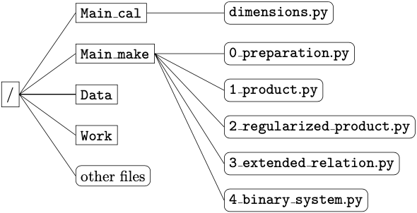
The executable files are in the directories named as and . The former contains five files that produce datas of binary systems (or binary matrices) obtained from the binary EDS relations, and the latter contains one file that calculates dimensions of and (or row echelon forms of the corresponding binary matrices). The produced datas are stocked in , almost of which are saved in Python pickle format to reduce data size. Class files in which essential precesses are performed are stored in . Files of config, license and readme are also placed in the root directory of the package. (See Figure 1 for a layout of the package).
We have a convenient expression for a linear combination in since consists of only two elements. A subset in is identified with a combination such as
| (4.4) |
For instance, corresponds to and corresponds to . By (4.4), the symmetric difference of two sets is equivalent to the plus of two combinations: corresponds to . The expression (4.4) is also applied to a linear relation in the same way. We compute binary EDS relations (or defining combinations in ) through (4.4) with the set datatype in Python. This set based expression can be realized by built-in objects.666 We use frozenset and s.symmetric_difference(t) (or the operator notation ‘s^t’), where frozenset is an immutable datatype for set datas and s,t are its instances.
We will explain the executable files and report their statics. We do not mention actual command lines to use the files in a linux OS, but we can find them in the beginning of each file.
4.1 Executable file in
We will require many maps to save midway datas for the binary linear systems induced from the binary EDS relations. The prime reason is that, by (2.6), each EDS relation is composed of a combination of , and . For the maps or the midway datas, we will use dictionary datatype, which is a built-in object in Python and consists of a collection of tuples of two objects called ‘key’ and ‘value’: a key-object is mapped to its associated value-object.
The file prepares two dictionary datas for each weight . Let denote the set for a positive integer . One data gives a one-to-one mapping from the integers in to the words of degree , and another data gives a one-to-one mapping from the integers in to the mult-indices in of weight : if and the associated mult-index is , the associated word is . The objects of the set which our programs select for the set based expression in the left of (4.4) are the integers (for which the integer datatype is necessary) instead of the mult-indices and words (for which the tuple and string datatypes are necessary), because the integer datatype is reasonable in data size and running time.
The file creates dictionary datas for shuffle and stuffle products. The defining equations (2.2) and (2.3) suggest that creating datas of shuffle will take more time since shuffle products can contain more terms. For a speed-up, we improve (2.2):
| (4.5) | |||||
where and . This is a spacial case of (2.2) if and can be proved by induction on . Let . Using (4.5) with , we can reduce shuffle products of weight to combinations of those of about half weight. We denote by and created datas of shuffle and stuffle, respectively. They map pairs of mult-indices to combinations including temporal indeterminates that are binary versions of regularized MZVs. For instance,
| (4.6) |
In the case of shuffle, for using (4.5) with , we also create maps from pairs of words to combinations of words up to weight . In those additional maps, we allow the words that can not be written in terms of mult-indices (e.g., and ).
Let be a mult-index that is expressed as , where and . Let denote a mult-index such that . By [19, Proposition 8],
| (4.7) |
Since the regularized MZV of is , its binary version should be
| (4.8) |
The dictionary datas that the file creates are obtained by applying (4.8) to ones that the previous file creates. For instance, we have by (4.8)
and so the previous datas in (4.6) are converted to
| (4.9) |
where and stand for the maps of regularized shuffle and stuffle, respectively.
The file makes binary EDS relations,
by combining the previous datas. For instance, the datas in (4.9) create the two relations,
The file converts the binary EDS relations of a weight to a binary linear system (which we call a binary EDS linear system) in both of text and pickle formats. The text format is organized as follows:
-
1.
A line with the first character ‘#’ is a comment line. Comment lines typically occur at the beginning of the file, but are allowed to appear throughout the file.
-
2.
The remainder of the file contains lines defining the binary linear relations, one by one.
-
3.
A relation is defined by positive integers numbering binary MZSs. A number ‘0’ is typically placed at the last of the line, but it is optional.
For example, the line “2 4 0” is corresponding to , if and are numbered as and , respectively. The pickle files are not necessary but useful: e.g., when loading the large size system. For Experiment 3.3, we also make binary and linear systems by restricting binary EDS relations.
The above programs run under the parallel process since the datas can be created independently if is divided into a plurality of blocks. The filenames of the datas by the parallel process have strings ‘’ at their tails. Editing the file we can control the max number of parallel threads.
In Table 5, we present computation times (or elapsed real times) to execute all files for , where stands for the -th file mentioned above from to . We find that calculating the regularizations in is the dominant process. Table 6 lists the file sizes of the binary linear systems in pickle format for , and . As expected from , the file of is smallest and that of EDS is largest for each weight. The size of text format file is about times the size of pickle one. For each weight , the maximum memory size (or maximum resident set size) to execute the files is the size required by , which is about half size used in Gaussian forward elimination (see Table 7). Computationally, making linear systems is not harder than calculating their coranks (or dimensions of cokernel) as we will see below.
| Total | ||||||
|---|---|---|---|---|---|---|
| 18 | 0 | 75 | 246 | 53 | 54 | 428 ( 7min) |
| 19 | 1 | 188 | 805 | 133 | 186 | 1313 ( 22min) |
| 20 | 3 | 469 | 3137 | 510 | 543 | 4662 ( 1.3hour) |
| 21 | 7 | 1529 | 15607 | 1384 | 2362 | 20889 ( 5.8hour) |
| 22 | 15 | 3018 | 61898 | 3675 | 6578 | 75184 ( 21hour) |
| EDS | |||
|---|---|---|---|
| 18 | 8.3M | 150M | 274M |
| 19 | 21M | 509M | 922M |
| 20 | 47M | 1.6G | 2.8G |
| 21 | 105M | 5G | 8.6G |
| 22 | 233M | 16G | 26G |
4.2 Executable file in
The file ( for short) executes the Gaussian forward elimination on a given binary linear system of a weight by using Algorithm A.6. In the process, an order of mult-indices (or binary MZSs) have to be determined to convert the inputted binary linear system into the corresponding binary matrix. We employ a sequence satisfying the following: if ,
-
(a)
; or
-
(b)
and .
The condition (a) means that the mult-indices (or columns in the corresponding matrix) are sectioned into blocks by depth: the mult-indices in a left block have a greater depth than those in a right block. The condition (b) means that the Hoffman mult-indices of depth are at the rightmost place in the th block. For example, the order of weight determined by , , and satisfies (a) and (b): they are sectioned as and the only Hoffman mult-index is located rightmost in the th block.
Proposition 4.1 is shown as follows.
Proof of Proposition 4.1. We consider the situation where
we run by inputing
the binary EDS linear system of weight . We then obtain a row echelon matrix satisfies the following.
-
(E1)
There exists a non-zero pivot at any column in .
-
(E2)
There exists no non-zero pivot at any column in .
For a non-zero combination in with , we define the leading term of by
By (a) and (b), the statements (E1) and (E2) are equivalent to (e1) and (e2), respectively:
-
(e1)
There exists a combination such that for any in .
-
(e2)
There exists no combination such that for any in .
Under (e1) and (e2), the back substitution (performed imaginarily) implies
Proposition 4.1,
where
the fact that
for any depth
is
used for (4.1).
We give examples of (4.3) for excluding the case that . Note that is always zero if and .
Examining the Gaussian forward elimination performed by in detail, we can find a part of the inputted binary EDS relations which forms a basis of . We give examples of bases for , where only the pairs of mult-indices are written (see Table 1 that lists associated relations for ).
-
.
-
, , .
-
, , , , , .
-
, , , , , , , , , , , , , .
We can verify Experiment 3.3 similarly to Experiment 3.2. We input and linear systems into . By Table 4, in most cases, row echelon matrices that do not satisfy (E1) are outputted. The fails of (E1) induce (3.7), and ensure Experiment 3.3.
The program in applies the parallel process to determine an order of mult-indices since mult-indices can be divided by depth. For instance, parallel threads occur as preprocessing if a binary EDS linear system of weight is inputted. Algorithm A.6, the main process for computing a row echelon matrix, is executed in single. It appears that the parallelization of Algorithm A.6 is not easy because a non-simple search procedure is incorporated.
In Table 7, we present the statics of the executions by whose inputs are the binary , and EDS relations. We observe that the computation for requires much more time than and EDS, although the number of relations of is quite small such that the corresponding matrix is square for any . This phenomenon expresses a characteristic of Algorithm A.6. It employs a conflict based search procedure inspired by the conflict-driven clause learning (CDCL), a modern method with many successes to practical applications in solving the Boolean satisfiability (SAT) problem. Roughly speaking, relations with good structures for finding conflict combinations can accelerate searching a pivot relation (see Remark A.7 for more information). The memory cost is bad in comparison with the statics in [21], but the runtime is about 10 times more faster. Therefore we can improve the record of calculating (3.2) from to by the use of a machine with large memory capacity.
| Rels | MeanNum | Memory | Time | |||
|---|---|---|---|---|---|---|
| 18 | 65536 | 65536 | 30.1 | 4.6G | 8.6hour | |
| \cdashline3-7 | 155711 | 230.4 | 7.3G | 8.8min | ||
| \cdashline3-7 | 188470 | 364.4 | 11.4G | 9.8min | EDS | |
| 19 | 131072 | 131072 | 33.7 | 16.5G | 68hour | |
| \cdashline3-6 | 327679 | 339.5 | 22.9G | 42.4min | ||
| \cdashline3-6 | 393206 | 523.1 | 34.3G | 43.7min | ||
| 20 | 262144 | 262144 | 37.6 | 61G | 22day | |
| \cdashline3-6 | 688254 | 500.5 | 82G | 5.3hour | ||
| \cdashline3-6 | 819316 | 751.7 | 110G | 4.7hour | ||
| 21 | 524288 | - | - | - | - | |
| \cdashline3-6 | 1441791 | 739.8 | 256G | 30hour | ||
| \cdashline3-6 | 1703925 | 1083.3 | 329G | 25hour | ||
| 22 | 1048576 | - | - | - | - | |
| \cdashline3-6 | 3014911 | 1094.4 | 789G | 8day | ||
| \cdashline3-6 | 3539188 | 1564.1 | 982G | 7day |
5 Problem
Some problems arise in connection with the experiments in Section 3.
Experiments 3.1 and 3.2 indicate typical problems on the dimensions of and : obviously, Problem 5.2 includes Problem 5.1.
Problem 5.1.
Does (3.1) hold for any weight ?
Experiment 3.3 yields the following:
Problem 5.3.
(i)
Is there a subset such that
and the sequence satisfies (3.8)?
(ii)
Can we find a law in the sequence ?
We have adopted the binary field for the scalar field of the formal multiple zeta space and for the computation of corank. (It is worth noting that the experiments of [21] employ and .) There are no particular reasons for choosing except computational science techniques are easy to apply. A discovery of a regularity of in Table 2 is a product of good luck.
Problem 5.4.
(i)
Can we find a theoretical reason
why
the dimensions have a Pascal triangle pattern?
(ii)
What will the dimensions be
if
we adopt other finite fields ?
Like MZVs, we can make an assumption that binary MZSs satisfy a multiplication compatible with the shuffle and stuffle products. Under the assumption, we have since . This means that the algebras of MZV and binary MZS are different. In particular, is not isomorphic to the polynomial ring in one variable, and statements and conjectures involving (e.g., those involving finite and symmetric multiple zeta values introduced in [20]) can not be varied to directly. It seems a mysterious problem that whether the algebra of binary MZS has a good property and a connection to the algebra of MZV.
Acknowledgements
The author would like to thank Tomohiro Sonobe for help with computing environments, and Junichi Teruyama for a recommendation to use (4.5) which made it possible to reduce computation costs. This work was supported by Japan Society for the Promotion of Science, Grant-in-Aid for Scientific Research (C) 20K03727.
Appendix
We will introduce a technique to speed up the Gaussian forward elimination over any field for a system of linear combinations that have some structure. An essential part of the technique appears in [24] to decide the full rankness of a binary matrix.
Let be variables, and we order the variables according to their subscripts. For a non-zero linear combination over , we denote by and the subscript and coefficient of the minimum variable, respectively. That is, and . We define and when .
In what follows we will handle mainly linear combinations over , and we just call them combinations. Let denote the -vector space spanned by combinations , and let . We say that is a pivot combination if , and
is a pivot sequence if and every is a pivot combination.
There are two key processes for the speed-up technique. One is a conflict search procedure.
Process A.1.
-
Input: Combinations and a pivot sequence .
-
Output: Either or such that
-
(a)
with ;
-
(b)
with and ;
-
(c)
; and
-
(d)
.
-
(a)
-
1.
Set and .
-
2.
Search from such that .
-
3.
Return if such exists.
-
4.
Return if .
-
5.
Evaluate .777 This evaluation is well-defined since and . The condition (d) follows from
-
6.
Set .
-
7.
Update , and go back to step .
Another is the classical elimination procedure with an evidence of conflict.
Process A.2.
-
Input: A pivot sequence and a pair which satisfies the output conditions in Process A.1.
-
Output: A combination such that .888 The theory of Gaussian elimination only ensures and . However, updating method of in step 2, together with the output conditions (c) and (d) in Process A.1, implies . It also implies . In fact, if , which is a contradiction. Therefore the output condition in Process A.2 holds.
-
1.
Set .
-
2.
For from to , update if .
-
3.
Return .
Process A.3.
Process A.3 is essential for finding a pivot combination whose minimum variable is , because we can find out it by Process A.3 if and only if it exists.
Proposition A.4.
For combinations
and
a pivot sequence ,
the following statements are equivalent.
(i)
Process A.3
outputs
such that .
(ii)
There exists a combination such that .
Proof.
Obviously,
(i) implies (ii).
Suppose
(ii) is true to prove the converse.
Then there exist elements
in such that
We have since is the minimum variable in .
We first consider the situation where we run Process A.1 for the inputs and : however, we temporally assume that step 3 is skipped and the process ends with the output at step 4 of . Let be the elements in which are recursively determined as at step , and let . Then , and
Since , this implies for some , which means that Process A.1 can find out in step 2 such that , at least when . Therefore, Process A.1 without the temporal assumption always outputs .
We input and into Process A.3. At step ,
we receive
from Process A.1. Thus
step 2 is skipped,
and
is received from Process A.2 at step 3,
which satisfies
the condition required in (i).
Since
is returned at step 4,
we conclude
(i) holds.
For a subscript and a pivot sequence with , we define
We call an integer in a deficient subscript, and a variable with a deficient variable.
We need to modify Process A.3 for practical use.
Process A.5.
-
Input: Combinations , a subscript , and a pivot sequence with .
-
Output: Either or a combination with .
-
1.
Change the variable order by moving the deficient variables backward.
-
2.
Prepare the pivot sequence for the new variable order.
-
3.
Receive from Process A.3 for the inputs and .
-
4.
Undo the variable order by putting the deficient variables back to their original places.
-
5.
Return .
We are in a position to state Algorithm A.6 for a fast Gaussian forward elimination.
Algorithm A.6.
-
Input: Combinations .
-
Output: A pivot sequence .
-
1.
Create subsets .
-
2.
Set and .
-
3.
Execute the following loop process to make a pivot sequence :
-
(i)
Update if ; otherwise break.
-
(ii)
If , append a combination in to and go back to (i).
-
(iii)
Receive from Process A.5 for the inputs and .
-
(iv)
If , go back to (i).
-
(v)
Append to ,999 The loop process ensures . To show this, we may prove by the output condition in Process A.5. Suppose and set . Then, on the -round in the loop process, Process A.5 at (iii) must return a non-zero combination by Proposition A.4 and the existence of , where note that Process A.5 is essentially Process A.3. This means a combination satisfying must be appended to at (v) on the -round, which contradicts . and back to (i).
-
(i)
-
4.
Return .
The pivot sequence outputted by Algorithm A.6 is a row echelon matrix under the order thanks to Proposition A.4 (see the footnote in (v) of step 3 for details).
Remark A.7.
Process A.1 is influenced by the unit propagation (UP) in the algorithm to solve the Boolean satisfiability (SAT) problem (see, e.g., [4, Chapter 1]). SAT is the first problem that was proved to be NP-complete, which means that all NP-problems are at most as difficult as SAT. UP is a technique to determine an assignment value for the variable we watch while searching a conflict combination (or a conflict clause in SAT terminology).
Process A.2 is inspired by the conflict-driven clause learning (CDCL) proposed in [3, 25, 26] (see also [4, Chapter 5]). CDCL enable us to find (or learn) a new pivot combination from the conflict evidence found by UP.
The performance of UP tends to increase when combinations have good structures for finding conflict combinations under a good variable order: i.e., not too few number of combinations, high frequency of small size combinations, bias of occurrences of variables, and so on. We have seen in Table 7 that the runtimes of and EDS are much better than those of , which seems to be due to the difference in numbers of relations (or combinations).
References
- [1]
- [2] H. Bachmann, Multiple zeta values and modular forms, Lecture notes (under construction, but available at https://www.henrikbachmann.com/mzv2020.html) in Nagoya University, Spring 2020.
- [3] R. J. Bayardo Jr. and R. C. Schrag, Using CSP look-back techniques to solve real-world SAT instances, Proceedings of the fourteenth national conference on artificial intelligence and ninth conference on Innovative applications of artificial intelligence, 203–208, 1997.
- [4] A. Biere, M. Heule, H. V. Maaren, and T. Walsh (eds.), Handbook of satisfiability, Frontiers in Artificial Intelligence and Applications, Volume 185, IOS Press, Amsterdam, The Netherlands, 2009.
- [5] M. Bigotte, G. Jacob, N. E. Oussous and M. Petitot, Lyndon words and shuffle algebras for generating the coloured multiple zeta values relations tables, Theor. Comput. Sci. 273 (2002), 271–282.
- [6] J. Blümlein, D. J. Broadhurst and J. A. M. Vermaseren, The multiple zeta value data mine, Comput. Phys. Commun. 181 (2010), 582–625.
- [7] D. Broadhurst and D. Kreimer, Association of multiple zeta values with positive knots via Feynman diagrams up to loops, Phys. Lett. B 393 (1997), 403–412.
- [8] F. Brown, Mixed Tate motives over , Ann. Math. 175 (2012), 949–976.
- [9] F. Brown, Depth-graded motivic multiple zeta values, Compos. Math. 157 (2021), 529–572.
- [10] P. Deligne and A. B. Goncharov, Groupes fondamentaux motiviques de Tate mixte, Ann. Sci. École Norm. Sup. 38 (2005), 1–56.
- [11] V. G. Drinfeld, On quasitriangular quasi-Hopf algebras and a group closely connected with , Leningrad Math. J. 2 (1991), 829–860.
- [12] M. Espie, J-C. Novelli and G. Racinet, Formal computations about multiple zeta values, in “From Combinatorics to Dynamical Systems” (Strasbourg, 2002), IRMA Lect. Math. Theor. Phys. 3, F. Fauvet and C. Mitschi (eds.), de Gruyter, Berlin, (2003), 1–16.
- [13] L. Euler, Meditationes circa singulare serierum genus, Novi Comm. Acad. Sci. Petropol. 20 (1776), 140–186 ; reprinted in Opera Omnia Ser. I, vol. 15, 217–267.
- [14] H. Furusho, The multiple zeta value algebra and the stable derivation algebra, Publ. Res. Inst. Math. Sci. 39 (2003), 695–720.
- [15] H. Gangl, M. Kaneko and D. Zagier, Double zeta values and modular forms, in “Automorphic forms and zeta functions”, Proceedings of the Conference in Memory of Tsuneo Arakawa, World Sci. Publ., Hackensack, NJ, (2006), 71–106.
- [16] A. B. Goncharov, Periods and mixed motives, preprint (arXiv:math/0202154), 2002.
- [17] M. Hirose and N. Sato, Iterated integrals on and a class of relations among multiple zeta values, Adv. Math. 348 (2019), 163–182.
- [18] M. E. Hoffman, The algebra of multiple harmonic series, J. Algebra 194 (1997), 477–495.
- [19] K. Ihara, M. Kaneko, and D. Zagier, Derivation and double shuffle relations for multiple zeta values, Compos. Math. 142 (2006), 307–338.
- [20] M. Kaneko, An introduction to classical and finite multiple zeta values, Publ. math. Besançon. Algèb. Théor. Nr. 1 (2019), 103–129.
- [21] M. Kaneko, M. Noro and K. Tsurumaki, On a conjecture for the dimension of the space of the multiple zeta values, Software for algebraic geometry 148 (2008), 47–58.
- [22] M. Kaneko and S. Yamamoto, A new integral-series identity of multiple zeta values and regularizations, Sel. Math. New Ser. 24 (2018), 2499–2521.
- [23] G. Kawashima, A class of relations among multiple zeta values, J. Number Theory 129 (2009), 755–788.
- [24] T. Machide and T. Sonobe, Determination method influenced by SAT solver for the full rankness of a matrix (in Japanese) , The 32nd Annual Conference of the Japanese Society for Artificial Intelligence, 2018.
- [25] J. P. Marques-Silva and K. A. Sakallah, GRASP – a new search algorithm for satisfiability, Proceedings of the 1996 IEEE/ACM international conference on Computer-aided design, 220–227, 1996.
- [26] J. P. Marques-Silva and K. A. Sakallah, GRASP: a search algorithm for propositional satisfiability, IEEE Transactions on Computers 48 (1999), 506–521.
- [27] H. N. Minh, G. Jacob, M. Petitot and N. E. Oussous, Aspects combinatoires des polylogarithmes et des sommes d’Euler-Zagier, J. Électr. Sém. Lothar. Combin. 43 (2000), Art. B43e, 29 pp.
- [28] H. N. Minh and M. Petitot, A Lyndon words, polylogarithms and the Riemann function, Discrete Math. 217 (2000), 273–292.
- [29] G. Racinet, Doubles mélanges des polylogarithmes multiples aux racines de l’unité, Publ. Math. IHÉS. 95 (2002), 185–231.
- [30] C. Reutenauer, Free Lie algebras, London Mathematical Society Monographs. New Series, 7. Oxford Science Publications. The Clarendon Press, Oxford University Press, New York, 1993.
- [31] K. Tasaka, On linear relations among totally odd multiple zeta values related to period polynomials, Kyushu J. Math. 70 (2016), 1–28.
- [32] T. Terasoma, Mixed Tate motives and multiple zeta values, Invent. Math. 149 (2002), 339–369.
- [33] R. Umezawa, Evaluation of iterated log-sine integrals in terms of multiple polylogarithms, preprint (arXiv:1912.07201 [math.NT]), 2019.
- [34] D. Zagier, Values of zeta functions and their applications, First European Congress of Mathematics, Vol. II (Paris, 1992), 497–512, Progr. Math., 120, Birkhuser, Basel. 1994.