Computer assisted proofs for transverse heteroclinics
by the parameterization method

J.D. Mireles James ¹¹1Florida Atlantic University, 777 Glades Rd., Boca Raton, FL 33431, USA. jmirelesjames@fau.edu J.M.J partially supported by NSF grant DMS - 2307987. Maxime Murray ²²2Florida Atlantic University, 777 Glades Rd., Boca Raton, FL 33431, USA. mmurray2016@fau.edu

Abstract

This work develops a functional analytic framework for making computer assisted arguments involving transverse heteroclinic connecting orbits between hyperbolic periodic solutions of ordinary differential equations. We exploit a Fourier-Taylor approximation of the local stable/unstable manifold of the periodic orbit, combined with a numerical method for solving two point boundary value problems via Chebyshev series approximations. The a-posteriori analysis developed provides mathematically rigorous bounds on all approximation errors, providing both abstract existence results and quantitative information about the true heteroclinic solution. Example calculations are given for both the dissipative Lorenz system and the Hamiltonian Hill Restricted Four Body Problem.

Key words. parameterization method, heteroclinic connecting orbits, dissipative systems, Hamiltonian systems, computer assisted proof

1 Introduction

This paper describes constructive, computer assisted arguments for proving theorems about cycle-to-cycle connecting orbits for ordinary differential equations. Our approach utilizes the parameterization method for stable/unstable manifolds attached to periodic orbits, as was developed in [26, 29, 50, 49, 12, 13, 41]. Validated numerical methods for Fourier, Taylor, and Chebyshev spectral approximations of these stable/unstable manifolds were developed (for example) in [33, 17, 61, 23, 30, 7, 37]. (See also the references therein).

The ideas described here are part of an ongoing program whose goal is to develop functional analytic tools for computer assisted proofs (CAPs) in nonlinear nonlinear analysis. The present work both builds on, and extends the ideas of [63, 59, 36, 32, 1, 2] on CAP for transverse heteroclinic and homoclinic connections between equilibrium solutions of vector fields, and the work of [45] on functional analytic CAPs for transverse homoclinic connections for periodic orbits in Hamiltonian systems. (Methods of CAP based on other methods are discussed briefly in Remark 1.2 below).

To facilitate the discussion, let $U\subset\mathbb{R}^{d}$ denote a connected open set and $f\colon U\to\mathbb{R}^{d}$ be a real analytic vector field. Suppose that $T>0$ , that $\lambda\in\mathbb{C}$ has nonzero real part, and that $P\colon\mathbb{R}\times[-\tau,\tau]\to\mathbb{R}^{d}$ is a smooth function, $T$ -periodic in its first variable, taking values in $U$ . If $P$ solves the partial differential equation equation

\frac{\partial}{\partial\theta}P(\theta,\sigma)+\lambda\sigma\frac{\partial}{\partial\sigma}P(\theta,\sigma)=f(P(\theta,\sigma)),

(1)

then the image of $P$ is a local stable or unstable manifold for a periodic orbit of the vector field $f$ .

To see this, note first that the image of $P$ is a cylinder, due to the periodicity of $P(\theta,\sigma)$ in its first variable. Next observe that the equator of the cylinder is a periodic solution of the differential equation $x^{\prime}=f(x)$ . To see this let $\gamma(\theta)=P(\theta,0)$ , and evaluate Equation (1) at $\sigma=0$ . This gives that

\frac{d}{d\theta}\gamma(\theta)=f(\gamma(\theta)),

as desired.

Assume now that $\mbox{real}(\lambda)<0$ . (The unstable case of $\mbox{real}(\lambda)>0$ is treated in a similar fashion). Define

x(t)=x(t,\theta,\sigma)=P(t+\theta,\sigma e^{\lambda t}),

with $t\geq 0$ and $\sigma\in[-\tau,\tau]$ . To see that $x(t)$ is on the stable manifold of $\gamma$ , one must show that $x(t)$ is an solution of the differential equation and then consider the limit as $t\to\infty$ .

Write $\bar{\sigma}=\sigma e^{\lambda t}$ and $\bar{\theta}=\theta+t$ . Then for $t>0$ and $\bar{\sigma}\in[-\tau,\tau]$ , we have that $(\bar{\theta},\bar{\sigma})$ is in the domain of $P$ , and

	$\displaystyle\frac{d}{dt}x(t)$	$\displaystyle=\partial_{1}P(t+\theta,\sigma e^{\lambda t})+\lambda\sigma e^{\lambda t}\partial_{2}P(t+\theta,\sigma e^{\lambda t})$
		$\displaystyle=\partial_{1}P(\bar{\theta},\bar{\sigma})+\lambda\bar{\sigma}\partial_{2}P(\bar{,}\bar{\sigma})$
		$\displaystyle=f(P(\bar{\theta},\bar{\sigma}))$
		$\displaystyle=f(x(t)).$

Here we pass from the second to the third line by applying the invariance equation (1).

Now we note that

	$\displaystyle\lim_{t\to\infty}\\|x(t,\theta,\sigma)-\gamma(t)\\|$	$\displaystyle=\lim_{t\to\infty}\\|P(t+\theta,\sigma e^{\lambda t})-P(t+\theta,0)\\|$
		$\displaystyle=0,$

so that the image of $P$ is a local stable manifold as desired. We refer to the curve $x(t)=x(t,\theta,\sigma)$ is a “whisker” of the periodic orbit, and that the whisker has asymptotic phase $\theta$ .

Note also that

\xi(\theta)=\frac{\partial}{\partial\sigma}P(\theta,0),

is the normal vector bundle (eigenfunction) associated with the Floquet multiplier $\lambda$ . To see this, observe that

\displaystyle\frac{\partial}{\partial\theta}P(\theta,\sigma)=f(P(\theta,\sigma))-\lambda\sigma\frac{\partial}{\partial\sigma}P(\theta,\sigma),

so that by taking the partial with respect to $\sigma$ , we have

	$\displaystyle\frac{\partial}{\partial\sigma}\frac{\partial}{\partial\theta}P(\theta,\sigma)$	$\displaystyle=\frac{\partial}{\partial\theta}\frac{\partial}{\partial\sigma}P(\theta,\sigma)$
		$\displaystyle=Df(P(\theta,\sigma))\frac{\partial}{\partial\sigma}P(\theta,\sigma)-\lambda\frac{\partial}{\partial\sigma}P(\theta,\sigma)-\lambda\sigma\frac{\partial^{2}}{\partial\sigma^{2}}P(\theta,\sigma).$

Evaluating at $\sigma=0$ and plugging in the definitions of $\xi(\theta)$ and $\gamma(\theta)$ , we see that

\frac{d}{d\theta}\xi(\theta)+\lambda\xi(\theta)=Df(\gamma(\theta))\xi(\theta),

which we recognize as the equation of first variation for the normal invariant vector bundle/eigenfunction associated with the Floquet multiplier $\lambda$ .

Now suppose that $P,Q$ are parameterizations of the local unstable and stable manifolds of a pair periodic orbits $\gamma_{1}$ and $\gamma_{2}$ and suppose that $y\colon[0,R]\to\Omega$ is an orbit segment which begins on the image of $P$ and terminates on the image of $Q$ . Then the orbit of any point on $y$ accumulates to $\gamma_{1}$ in backward time, to $\gamma_{2}$ in forward time, and hence is a heteroclinic connection from $\gamma_{1}$ to $\gamma_{2}$ . Such an orbit segment can be seen as a zero of the operator equation

F(y,\alpha,\beta,T)=\left(\begin{array}[]{c}y(t)-P(\alpha)-\int_{0}^{t}f(y(s))\,ds\\ Q(\beta)-\int_{0}^{T}f(y(s))\,ds\end{array}\right),

where $\alpha,\beta$ are coordinates on the stable/unstable manifolds.

Appropriate phase conditions, and transversality are discussed in Section 3, where we project this functional equation, and the appropriate functional equations for for the parameterized manifolds, into Banach spaces of rapidly decaying coefficient sequences. The main point at the moment is that the parameterizations $P$ and $Q$ allow us to formulate two point boundary value problems (BVP) describing the connecting orbits, and that these BVPs can be studied using well established methods of computer assisted proof. See for example [52, 51, 47, 66, 5, 72, 67, 63, 60].

In the remainder of the paper, we describe the method and its application in both dissipative and Hamiltonian systems (these require different phase conditions). We illustrate its utility for both polynomial and nonpolynomial systems. Our computational method and a-posteriori validation schemes for the periodic orbits and their local stable/unstable manifolds are discussed in Section 2 with the validation of the connecting orbits discussed in Section 3. Example applications are presented in Section 4. A number of technical details are developed in the Appendices A, B, and C. But before moving on to these developments, we first provide a few additional remarks and then introduce the main example applications studied in the present work.

Remark 1.1 (Solving Equation (1)).

There are at lest two common approaches to solving Equation (1). The first is to treat it as an “elliptic” equation, and solve “all at once” via some iterative scheme. The second is to make a power series ansatz

P(\theta,\sigma)=\sum_{n=0}^{\infty}p_{n}(\theta)\sigma^{n},

for the solution, and to derive the homological equations satisfied by the coefficient functions $p_{n}(\theta)$ . These homological equations turn out to be linear ODEs, and one can solve them recursively. When pursuing this later approach, the calculations above determine the solution $P$ to first order.

It is the order-by-order approach which we adopt below, and we note that it has been exploited in earlier computer assisted proofs for the parameterization method, in a number of different contexts. See for example [63, 36, 31, 45, 13] and also the lecture notes of [40]. Validated computer assisted error bounds for the “elliptic” or “all-in-one-go” approach of (i) are discussed in detail in [53, 39].

Remark 1.2 (Literature on CAP for connecting orbits).

To the best of our knowledge, the first computer assisted proof of chaotic dynamics appeared in the early 1990’s [48]. The paper considered the area preserving Taylor-Greene-Chirikov Standard map, and the proof exploited the homoclinic tangle theorem of Smale [54]. In this approach, the main steps in the argument involved establishing the existence of a transverse homoclinic intersection between the (one dimensional) stable and unstable manifolds of the map’s hyperbolic fixed point.

By the late 1990’s and early 2000’s a number of authors had developed computer assisted arguments using topological tools – like either Conley or Brower indices – and applied them to prove theorems about chaotic dynamics in both discrete and continuous time dynamical systems. For example the papers [77, 76, 78] provided proofs of chaotic dynamics in the Henon map and in a Poincaré section of the Rössler system. Extensions to non-uniformly hyperbolic chaotic sets like in the Lorenz and Chua circuit are found in [19, 18, 21, 42, 43, 44]. More recently, topological techniques for CAP have also been extended to infinite dimensional systems like population models with spatial dispersion [14, 16] and parabolic partial differential equations [73].

The methods just cited establish the existence of chaotic invariant horseshoes via direct topological covering arguments. The resulting sets may however not be attracting. Geometric/topological techniques for proving theorems about chaotic attractors were first developed in [55, 56] to resolve Smale’s 14th question. Extensions of these methods are found in [70, 20].

Finally we mention that computer assisted methods of proof for heteroclinic and homoclinic solutions of ODEs based on geometric/topological methods have a long history as well. For example, the papers [75, 22] describe a geometric approach based on covering relations/cone conditions, and apply this approach to the Henon systems. Extensions to some problems in Celestial mechanics and to the Michelson system are given in [71, 72, 67, 68, 69].

A method which also leads to transversality is developed, and applied to problems in Celestial Mechanics (similar to the problems considered here) in [9]. We also mention that topological/geometric methods for studying Arnold diffusion in Celestial Mechanics problems have been developed in [10]. A study of the connecting orbit structure of the Swift-Hohenberg PDE using Conley index/connection matrix techniques is in the work of [15].

Of course the preceding light review is far from comprehensive, and the interested reader will find many additional references and a much more complete discussion by consulting the papers cited above. For more information, we also refer to the review articles of [58, 24] and to the books of [57, 62, 46].

1.1 Two Example Problems

The functional analytic setup for heteroclinic connections in dissipative systems is a little different from the setup required in the Hamiltonian setting. To illustrated each, we fix a particular dissipative and Hamiltonian example problem.

1.1.1 A Dissipative Example: The Lorenz System

The Lorenz system is a three parameter family of quadratic vector fields on $\mathbb{R}^{3}$ given by

$\displaystyle x^{\prime}$	$\displaystyle=\sigma(y-x)$	(2)
$\displaystyle y^{\prime}$	$\displaystyle=x(\rho-z)-y$	(3)
$\displaystyle z^{\prime}$	$\displaystyle=xy-\beta z$	(4)

where the “classic” parameter values studied by Edward Lorenz in 1963 are $\rho=28$ , $\sigma=10$ , and $\beta=8/3$ [38]. The system is an extremely simplified toy model of atmospheric convection and, perhaps more importantly, has become an iconic example of a simple nonlinear system exhibiting rich dynamics.

We note that the system is dissipative (contracts phase space volume in forward time) as can be seen by computing the determinant of the Jacobian matrix of the vector field. So periodic solutions, when they exist, tend to be isolated. More precisely, two periodic orbits may be very close together in the phase space, but in this case they will have very different periods. So, when computing periodic a solution the frequency or period of the orbit is one of the unknowns.

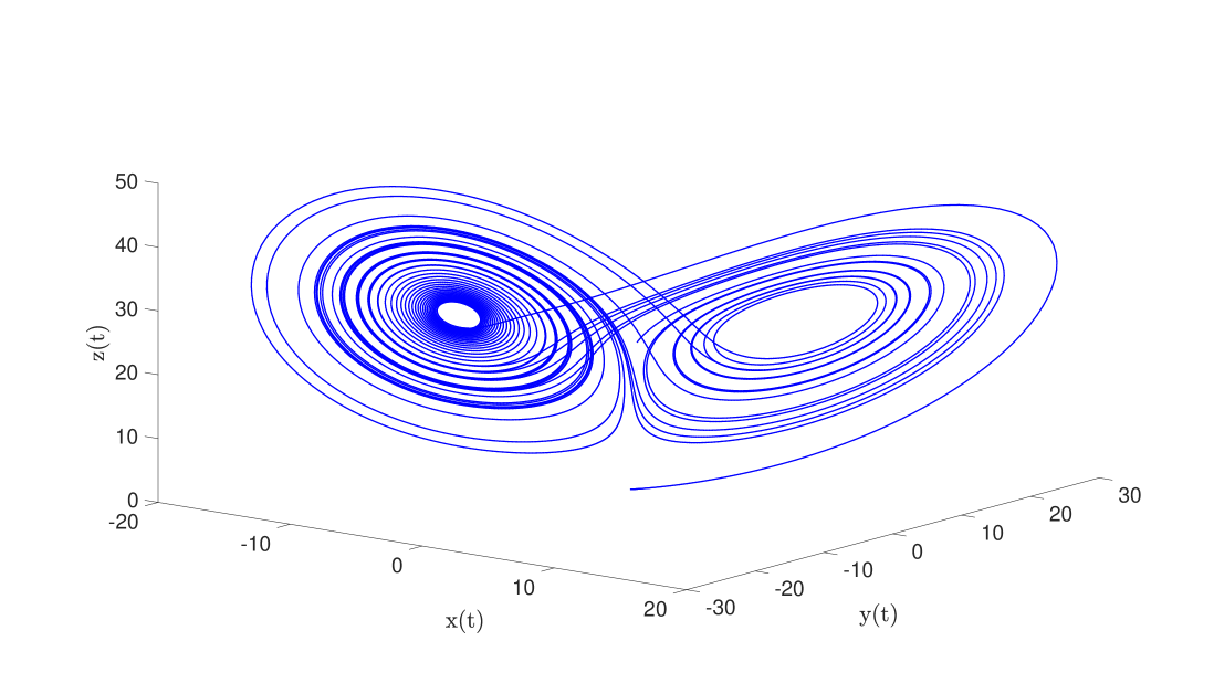
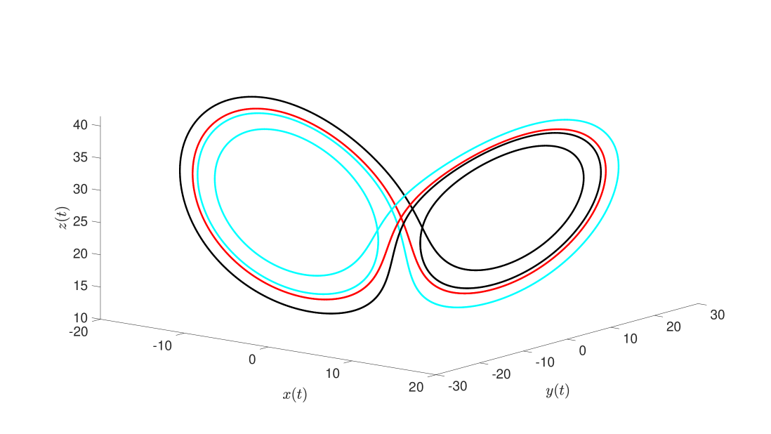
For many parameter values (including the classic parameters recalled above) the dominant feature of the phase space of Equation (2) is the so called Lorenz attractor, illustrated in the top frame of Figure 1. Qualitative properties of the dynamics on the attractor are discussed in detail in [74, 25, 4, 3]. A constructive proof of the existence of the Lorenz attractor at the classic parameter values, along with direct verifications of many of its properties was given by Warwick Tucker in 1999 [55, 56].

From the point of view of the present work, what is important is that hyperbolic periodic orbits are dense in the attractor, and that we should typically expect heteroclinic and homoclinic connections between them. The bottom frame of Figure 1 illustrates three of the shortest periodic orbits on/near the attractor, and highlights the fact that they do provide a skeleton of its shape. These orbits are coded by $AB$ , $AAB$ , and $ABB$ where an $A$ or $B$ represents a wind around the left or right lobe of the attractor. As an illustration the utility of the techniques described in the present work, we prove the existence of these periodic orbits and establish the existence of transverse heteroclinic connections between them.

Refer to caption — Figure 1: (Top) Illustration of the Lorenz attractor obtained by integrating a single initial condition. Here we chose an initial condition near the origin, but this is incidental. (Bottom) Three periodic orbits of the Lorenz system at the classic parameter values. Note that these three periodic orbits already give a strong impression of the shape of the Lorenz attractor.

1.1.2 A Hamiltonian Example: A Lunar Hill Problem

Many Hamiltonian systems are periodic orbit rich. In some cases this is because the system is a perturbation of an integrable system, and many periodic orbits will survive the perturbation. In other cases, it may be that Poincare recurrence holds in some energy level set, so that periodic orbits are in fact dense. In any event, periodic orbits in systems preserving first integrals generically occur in one parameter families or “tubes”, and extra care is needed to isolate an orbit.

We the system of differential equations given by

$\displaystyle x^{\prime}$	$\displaystyle=p$
$\displaystyle y^{\prime}$	$\displaystyle=q$	(5)
$\displaystyle p^{\prime}$	$\displaystyle=\lambda_{2}x+2q-\frac{x}{\left(x^{2}+y^{2}\right)^{3/2}}$
$\displaystyle q^{\prime}$	$\displaystyle=\lambda_{1}y-2p-\frac{y}{\left(x^{2}+y^{2}\right)^{3/2}}.$

Here

\lambda_{1}=\frac{3}{2}(1-d),\quad\quad\quad\lambda_{2}=\frac{3}{2}(1+d),

and

d=\sqrt{1-3\mu+3\mu^{2}}.

We refer to Equation (1.1.2) as the Hill equilateral restricted four body problem (HRFBP), and note that it reduces to the standard lunar Hill problem when $\mu=0$ . The HRFBP has the continuous symmetry

J(x,y,p,q)=\lambda_{2}x^{2}+\lambda_{1}y^{2}-p^{2}-q^{2}+\frac{2}{\sqrt{x^{2}+y^{2}}},

which is referred to as the Jacobi integral.

Equation (1.1.2) was derived by Burgos and Gidea in [6], and describes the dynamics of an infinitesimal particle (like a small rock or man-made satellite) moving in the vicinity of a large astroid. The astroid participates in a three body equilateral triangle relative equilibrium (Lagrangian triangle), in the following sense. We assume that there are three massive gravitating bodies $m_{1}\gg m_{2}\gg m_{3}>0$ , where $m_{3}$ is the mass of the astroid, and that these three bodies orbit their common center of mass on Keplerian circles in such a way that - in an appropriate co-rotating frame - the three bodies form the vertices of an equilateral triangle. The two larger massive bodies $m_{1}$ and $m_{2}$ are “sent to infinity” in such a way that their influence is still felt at $m_{3}$ , which is located at the origin. The parameter $\mu=m_{1}/(m_{1}+m_{2})$ describes the mass ratio of the two massive bodies at infinity. Note that $\mu\in[0,1/2]$ as $\mu=1$ when $m_{2}=0$ and $\mu=1/2$ when $m_{2}=m_{1}$ .

This kind of configuration actually occurs in our solar system, for example with $m_{1}$ the Sun, $m_{2}$ Jupiter, and $m_{3}$ a Trojan astroid like Hector, so that the orbits of Equation (1.1.2) would describe the dynamics of a satellite maneuvering close enough to Hector that the effects of the Sun and Jupiter can be considered as small. Other configurations exist involving Jupiter and its moons.

The system has four equilibrium solutions, also known as libration points, two of which are on the $x$ -axis and are denoted by $L_{1}$ and $L_{2}$ . These are located at

L_{1}=\left(\frac{1}{\lambda_{2}^{1/3}}\right),\quad\quad\mbox{and}\quad\quad L_{2}=\left(\frac{-1}{\lambda_{2}^{1/3}}\right).

The other two equilibria located on the $y$ -axis denoted by $L_{3}$ and $L_{4}$ and located at

L_{3}=\left(\frac{1}{\lambda_{1}^{1/3}}\right),\quad\quad\mbox{and}\quad\quad L_{4}=\left(\frac{-1}{\lambda_{1}^{1/3}}\right),

play no role in the present work.

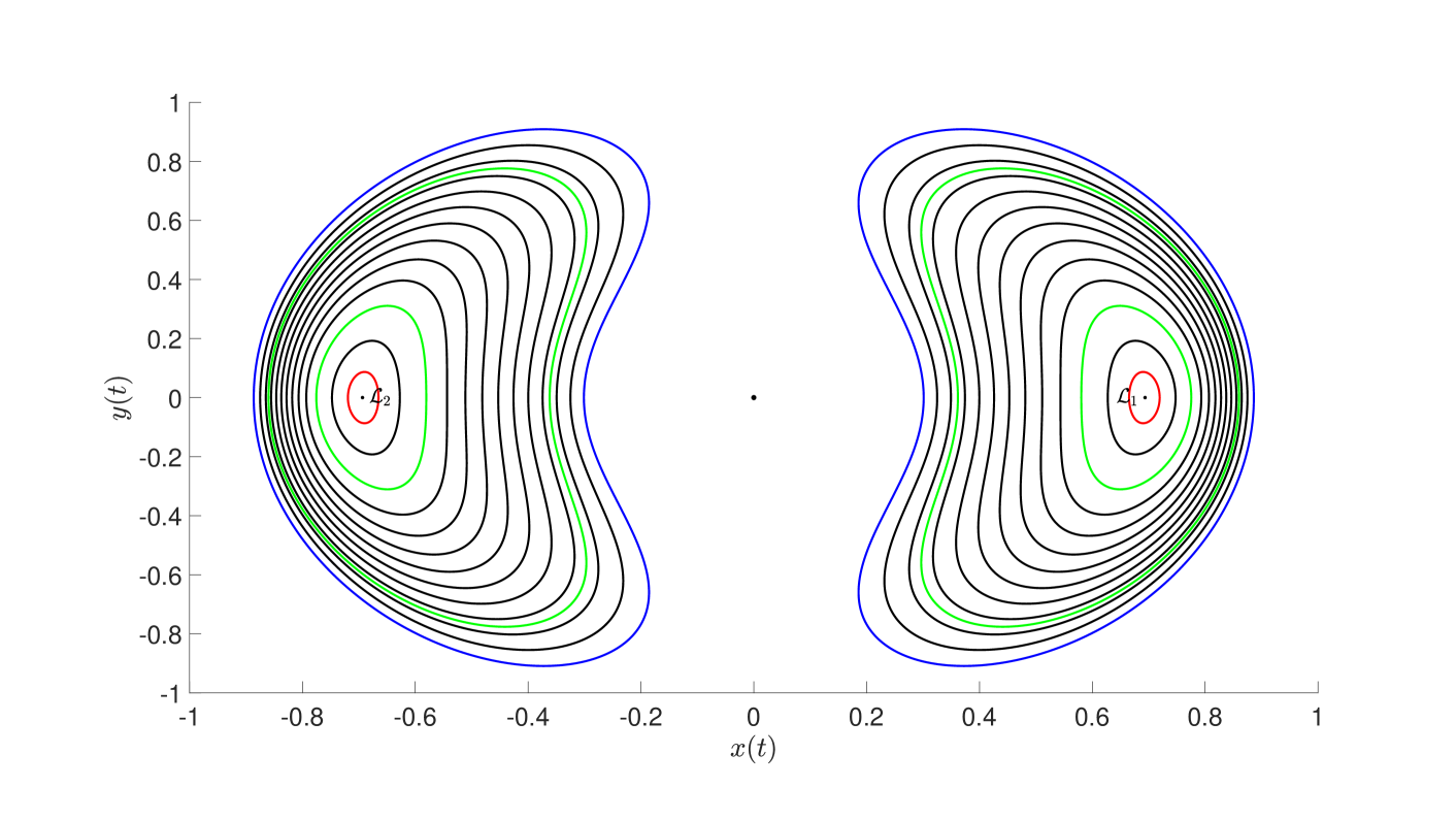
While the stability type of $L_{3}$ and $L_{4}$ depend on the mass ratio $\mu$ , $L_{1,2}$ have saddle-center stability for all values of $\mu\in(0,1/2]$ . The center eigenvalues at $L_{1}$ and $L_{2}$ give rise to a Lyapunov family of periodic orbits, locally parameterized by the Jacobi integral. For energies near the energy of $L_{1,2}$ , the Lyapunov orbits inherit one stable and one unstable Floquet multipliers from the stable/unstable directions of $L_{1,2}$ , and hence have attached stable/unstable manifolds. The stable/unstable manifolds of these periodic orbits could in turn intersect in the energy level set, giving rise to chaotic dynamics.

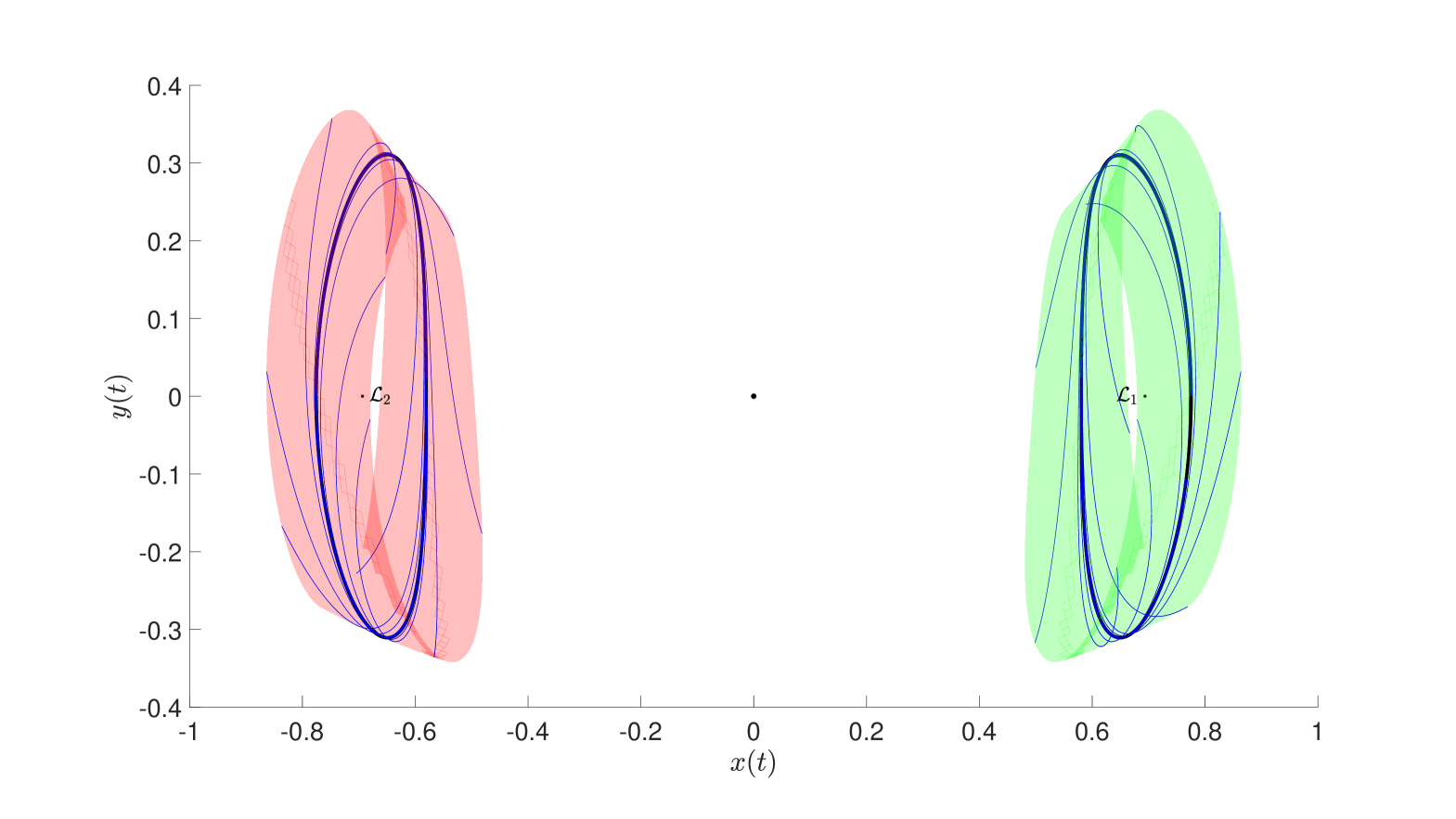
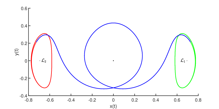
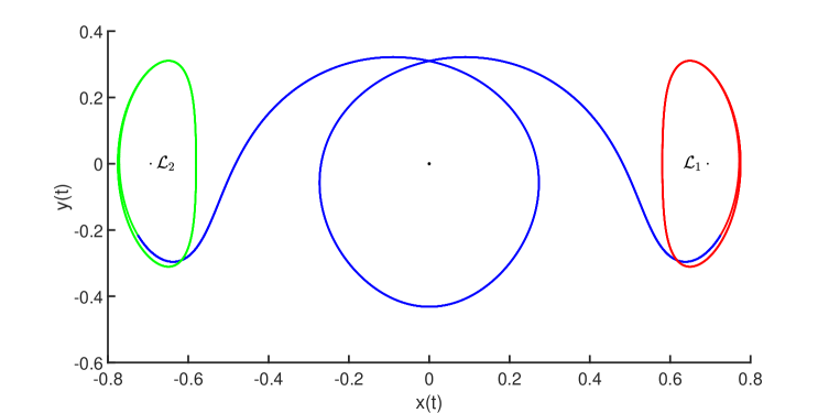
In Figure 2, we illustrate a number of periodic orbits in the Lyapunov families of $L_{1,2}$ , for some selected values of the Jacobi integral. The small and large green orbits are at a the same energy levels, and establish the existence of heteroclinic connections between some of these (and some others) below.

Remark 1.3 (Polynomial Embedding).

The methods of the present work rely heavily on formal series manipulations which are much simpler when we work with polynomial nonlinearities. For this reason, we will derive a vector field which is somehow equivalent to Equation (1.1.2), but which has only polynomial nonlinearities. This can be done using an embedding technique discussed in detail in [8, 28, 32].

The idea is to introduce new variables for the non-polynomial terms, and append polynomial differential equations describing these nonlinearities. Since the elementary functions of mathematical physics themselves solve simple (usually polynomial) differential equations, this idea applies to many of the examples which arise in practice. The cost of this embedding is that we increase the dimension of the system by a number which depends on the complexity of the non-polynomial terms.

To see this idea at work in the HRFBP, we begin by letting

r=x^{2}+y^{2},

so that

z(r)=(x^{2}+y^{2})^{-1/2}=r^{-1/2}.

Note that $z(r)$ generates the non-polynomial part of Equation (1.1.2) in the following sense. Differentiating obtains

	$\displaystyle z^{\prime}$	$\displaystyle=-\frac{1}{2}r^{-3/2}(2x^{\prime}x+2y^{\prime}y)$
		$\displaystyle=-(r^{-1/2})^{3}(xx^{\prime}+yy^{\prime})$
		$\displaystyle=-z^{3}(xx^{\prime}+yy^{\prime}).$

Combining this with Equation (1.1.2), and making the appropriate substitutions, we have

$\displaystyle x^{\prime}$	$\displaystyle=p$
$\displaystyle y^{\prime}$	$\displaystyle=q$
$\displaystyle p^{\prime}$	$\displaystyle=\lambda_{2}x+2q-xz^{3}$
$\displaystyle q^{\prime}$	$\displaystyle=\lambda_{1}y-2p-yz^{3}$
$\displaystyle z^{\prime}$	$\displaystyle=-z^{3}(xp+yq).$	(6)

Now, given initial conditions $(x_{0},p_{0},y_{0},q_{0})\in\mathbb{R}^{4}$ , we require that

z(0)=z_{0}=\frac{1}{\left(x_{0}^{2}+y_{0}^{2}\right)^{1/2}}.

Note that if $x$ , $y$ are non-zero, then this constraint is equivalent to

\left(x_{0}^{2}+y_{0}^{2}\right)^{1/2}z_{0}=1,

or, after squaring

\left(x_{0}^{2}+y_{0}^{2}\right)z_{0}^{2}=1.

(7)

We can easily check that, for any orbit which does not pass through $x=y=0$ (collision) the first four components of a solution of Equation (1.3) provide a solution to Equation (1.1.2). Note that if $x=y=0$ in Equation (1.3), then we cannot reverse the derivation of the constraint Equation (7). That is, the constraint on the initial condition carries the singularity of the original problem (i.e. this polynomial embedding technique, despite first appearances, is not a regularization technique).

2 Validated numerics for the parameterization method

The first step in our approach is to project the problems into appropriate spaces of Fourier, Fourier-Taylor, and Chebyshev series coefficients. This reduces the ordinary and partial differential equations describing periodic orbits, normal vector bundles, parameterized invariant manifolds, and connecting orbits to systems of infinitely many algebraic equations. By truncating these algebraic equations and applying numerical Newton schemes, we obtain the approximate solutions around which we construct our a-posteriori arguments.

The first step is to study the order zero and one terms in $P$ , the solution of equation (1) expressed using a power series in its second variable. That is, the periodic orbit, its Floquet multiplier and associated normal bundle. We begin by looking for $\gamma$ periodic having Fourier expansion

\gamma(t)=\sum_{k\in\mathbb{Z}}a_{0,k}e^{ik\omega t},

where $a_{0,k}\in\mathbb{C}^{n}$ and $\omega=2\pi/T$ . Here, the zero in the subscript denotes the fact that the periodic orbit is the zero-th order term in stable/unstable manifold expansion described in Section 1.

In application problems we are interested in real valued $\gamma$ , so that $a_{0,k}=\mbox{conj}(a_{0,-k})$ for all $k\in\mathbb{Z}$ . Moreover $\gamma$ is analytic (as $f$ is analytic in a neighborhood of $\Gamma=\{\gamma(t):t\in[0,T]\}$ ), and the Fourier coefficients decay exponentially fast, and there is a $\nu>1$ so that $\{a_{k}\}_{k\in\mathbb{Z}}\in(\ell_{\nu}^{1})^{n}$ .

Noting that

\frac{d}{dt}\gamma(t)=\sum_{k\in\mathbb{Z}}i\omega ka_{0,k}e^{i\omega kt},

and letting

f(\gamma(t))=\sum_{k\in\mathbb{Z}}q_{k}e^{i\omega kt},

where the $q_{k}$ depend on the $a_{0,k}$ , we have that a periodic orbit can be viewed as a solution of the equation

\sum_{k\in\mathbb{Z}}i\omega ka_{0,k}e^{i\omega kt}=\sum_{k\in\mathbb{Z}}q_{k}e^{i\omega kt}.

Since two smooth periodic functions are equal if and only if the coefficients of their Fourier expansions are equals, matching like-terms leads to the infinite system of algebraic equations

i\omega ka_{0,k}e^{i\omega kt}-q_{k}(a_{0})=0,\quad\quad\quad\quad k\in\mathbb{Z},

where $a_{0}=\{a_{0,k}\}_{k\in\mathbb{Z}}$ .

The problem requires the addition of a phase condition to remove infinitesimal rotations and isolate a unique solution in the space of Fourier coefficients. In this work, we choose a relaxed Poincaré type condition by defining a co-dimension one plane in $\mathbb{R}^{n}$ and requiring that $\gamma(0)$ is in this plane. More precisely, we choose $\bar{\gamma}_{0}\in\mathbb{R}^{3}$ and $\bar{\gamma}_{1}=f(\bar{\gamma}_{0})$ , defining

F_{0}^{0}(a_{0})=\bar{\gamma}_{1}-\sum_{i=1}^{n}\left(\bar{\gamma}_{0}^{i}\cdot\sum_{|k|<K_{0}}a_{0,k}^{i}\right).

(8)

Taking $K_{0}\in\mathbb{N}$ yields a finite dimensional condition in Fourier space.

Example 2.1 (Periodic solutions of the Lorenz system in Fourier space).

Finding a periodic orbit for the Lorenz system is equivalent finding a zero $(\omega,a_{0}^{1},a_{0}^{2},a_{0}^{3})\in\mathbb{R}\times\ell_{\nu}^{1}\times\ell_{\nu}^{1}\times\ell_{\nu}^{1}$ of the map $F_{0}=(F_{0}^{0},F_{0}^{1},F_{0}^{2},F_{0}^{3})$ whose components are given by

F_{0}(\omega,a_{0}^{1},a_{0}^{2},a_{0}^{3})=\begin{pmatrix}F_{0}^{0}(a_{0}^{1},a_{0}^{2},a_{0}^{3})\\ \left\{-i\omega ka_{0,k}^{1}+\sigma a_{0,k}^{2}-\sigma a_{0,k}^{1}:k\in\mathbb{Z}\right\}\\ \left\{-i\omega ka_{0,k}^{2}+\rho a_{0,k}^{1}-a_{0,k}^{2}-(a_{0}^{1}\ast a_{0}^{3})_{k}:k\in\mathbb{Z}\right\}\\ \left\{-i\omega ka_{0,k}^{3}-\beta a_{0,k}^{3}+(a_{0}^{1}\ast a_{0}^{2})_{k}:k\in\mathbb{Z}\right\}\end{pmatrix},

(9)

where $F_{0}^{0}$ is as given in (8) with $n=3$ . The equation $F=0$ is studied in detail in [30], where a number of computer aided proofs for periodic orbits in the Lorenz system are implemented. In particular the truncated problem, the application of Theorem A.1, and the operators $A$ and $A^{\dagger}$ introduced to compute the polynomial bound $Z(r)$ are discussed in detail. We employ these techniques in the present work as well.

Example 2.2 (Periodic solutions of Hill’s three-body problem in Fourier space).

In the case of Hill’s three-body problem, we require two additional scalar phase conditions to isolate a unique solution. First, we impose the scalar constraint from Equation (7), in order to guarantee equivalence between the polynomial and non-polynomial problems. Second, due to the fact that periodic solutions occur in one parameter families parameterized by energy/frequency, we fix the value of the Jacobi integral to some $C\in\mathbb{R}$ . Of course, to balance the resulting system, we must include two additional unfolding parameters into our zero finding problem. The unfolding parameters associated with the energy level and initial conditions are discussed in detail in [8, 11], and we use the same ideas below.

More precisely, set

A_{0}^{i}\,\stackrel{{\scriptstyle\mbox{\tiny{\raisebox{0.0pt}[0.0pt][0.0pt]{def}}}}}{{=}}\,\sum_{k\in\mathbb{Z}}a_{0,k}^{i},\quad 1\leq i\leq 5.

Fixing $\bar{\gamma}_{1},\bar{\gamma}_{0}^{i}\in\mathbb{R}^{n}$ , for $i=1,\ldots,5$ , and $C\in\mathbb{R}$ defining the desired energy level set, the three phase conditions are encoded in the map $F_{0}^{0}$ defined by

F_{0}^{0}(a_{0}^{1},a_{0}^{2},a_{0}^{3},a_{0}^{4},a_{0}^{5})=\begin{pmatrix}\bar{\gamma}_{1}-\displaystyle\sum_{i=1}^{5}\left(\bar{\gamma}_{0}^{i}\cdot\sum_{|k|<K_{0}}a_{0,k}^{i}\right)\\ (A_{0}^{5})^{2}\left[\left(A_{0}^{1}\right)^{2}+\left(A_{0}^{2}\right)^{2}\right]-1\\ \lambda_{2}\cdot\left(A_{0}^{1}\right)^{2}+\lambda_{1}\cdot\left(A_{0}^{2}\right)^{2}-\left(A_{0}^{3}\right)^{2}-\left(A_{0}^{4}\right)^{2}+2\cdot A_{0}^{5}-C\end{pmatrix}.

The additional scalar variables are included into the system through the map

G_{0}(\beta_{1},\beta_{2},a_{0})=\begin{pmatrix}0\\ 0\\ 0\\ \left\{\beta_{1}a_{0,k}^{1}:k\in\mathbb{Z}\right\}\\ \left\{\beta_{1}a_{0,k}^{2}:k\in\mathbb{Z}\right\}\\ \left\{\beta_{1}a_{0,k}^{3}:k\in\mathbb{Z}\right\}\\ \left\{\beta_{1}a_{0,k}^{4}:k\in\mathbb{Z}\right\}\\ \left\{\beta_{1}a_{0,k}^{5}+\beta_{2}(a_{0}^{5}\ast a_{0}^{5}\ast a_{0}^{5})_{k}:k\in\mathbb{Z}\right\}\end{pmatrix}.

Now our goal is to find $(\omega,\beta_{1},\beta_{2},a_{0})\in\mathbb{R}\times\mathbb{R}\times\mathbb{R}\times(\ell_{\nu}^{1})^{5}$ so that $F(\omega,\beta_{1},\beta_{2},a_{0})=F_{0}(\omega,a_{0})+G_{0}(\beta_{1},\beta_{2},a_{0})=0$ , where $F_{0}$ is given by

F_{0}(\omega,a_{0})=\begin{pmatrix}F_{0}^{0}(a_{0}^{1},a_{0}^{2},a_{0}^{3},a_{0}^{4},a_{0}^{5})\\ \left\{-i\omega ka_{0,k}^{1}+a_{0,k}^{3}:k\in\mathbb{Z}\right\}\\ \left\{-i\omega ka_{0,k}^{2}+a_{0,k}^{4}:k\in\mathbb{Z}\right\}\\ \left\{-i\omega ka_{0,k}^{3}+2a_{0,k}^{4}+\lambda_{2}a_{0,k}^{1}-(a_{0}^{1}\ast a_{0}^{5}\ast a_{0}^{5}\ast a_{0}^{5})_{k}:k\in\mathbb{Z}\right\}\\ \left\{-i\omega ka_{0,k}^{4}-2a_{0,k}^{3}+\lambda_{1}a_{0,k}^{2}-(a_{0}^{2}\ast a_{0}^{5}\ast a_{0}^{5}\ast a_{0}^{5})_{k}:k\in\mathbb{Z}\right\}\\ \left\{-i\omega ka_{0,k}^{5}-(a_{0}^{1}\ast a_{0}^{3}\ast a_{0}^{5}\ast a_{0}^{5}\ast a_{0}^{5})_{k}-(a_{0}^{2}\ast a_{0}^{4}\ast a_{0}^{5}\ast a_{0}^{5}\ast a_{0}^{5})_{k}:k\in\mathbb{Z}\right\}\end{pmatrix}

(10)

Moreover if $(\omega,\beta_{1},\beta_{2},a_{0})$ is a zero of $F$ , then $\beta_{1}=\beta_{2}=0$ , so that we are actually solving Equation (1.3). This can be shown precisely as in [8, 11].

Next, we study the linear stability of the periodic orbit $\gamma(t)$ by finding an invariant (stable/unstable) vector bundle $v(t)$ and associated Floquet exponent $\lambda\in\mathbb{C}$ for $\gamma$ . The pair $(\lambda,v)$ solves the linear equation

\dot{v}(t)+\lambda v(t)-A(t)v(t)=0,

(11)

where $A(t)=Df(\gamma(t))$ is the differential of the vector field evaluated along the periodic orbit.

In the present work we study periodic orbits with only one stable or unstable exponent. Then the stable/unstable bundle provides a linear approximation of the local stable/unstable manifold attached to the periodic orbit $\gamma$ . In the problems studied in this work, the stable/unstable bundles are periodic with period $T$ . (This is the orientable case. In the non-orientable case the bundle has period $2T$ , a scenario not treated here but which would require only a minor modification to the setting presented in the current section).

Example 2.3 (Normal bundles in the example system).

In the case of the Lorenz system, we have that

A(t)=Df(\gamma(t))=\left(\begin{array}[]{c c c}-\sigma&\sigma&0\\ \rho-\gamma^{(3)}(t)&-1&-\gamma^{(1)}(t)\\ \gamma^{(2)}(t)&\gamma^{(1)}(t)&-\beta\end{array}\right).

We note that, after expanding each periodic function as a Fourier series, the coordinates with products can be written with the use of Cauchy-Convolution products, such as introduced in Definition 9. It follows that the Fourier coefficients $a_{1}=(a_{1}^{1},a_{1}^{2},a_{1}^{3})$ of $v(t)$ satisfying (11) are a zero of

F_{1}(\lambda,a_{1})=\begin{pmatrix}F_{1}^{0}(a_{1})\\ \left\{-i\omega ka_{1,k}^{1}+\sigma a_{1,k}^{2}-\sigma a_{1,k}^{1}:k\in\mathbb{Z}\right\}\\ \left\{-i\omega ka_{1,k}^{2}+\rho a_{1,k}^{1}-a_{1,k}^{2}-(a^{1}\star a^{3})_{1,k}:k\in\mathbb{Z}\right\}\\ \left\{-i\omega ka_{1,k}^{3}-\beta a_{1,k}^{3}+(a^{1}\star a^{2})_{1,k}:k\in\mathbb{Z}\right\}\end{pmatrix}.

We note that the presentation use $a_{0}$ , the Fourier coefficients of the periodic orbit, to present the operator with Cauchy-Convolution product. But the coefficients $a_{0}$ are fully determined by solving the previous operator introduced in Example 2.1. The first coordinate, $F_{1}^{0}(a_{1})$ , is a scalar equation fixing the magnitude of the tangent bundle at $t=0$ to guarantee that the desired solution is well isolated. This scalar restriction also has the effect of balancing the unknown eigenvalue $\lambda$ . This equation can be relaxed to a finite dimensional restriction. In this work, we take

F_{1}^{0}(a_{1})=\sum_{i=1}^{3}\left(\sum_{|k|<k_{0}}a_{1,k}^{i}\right)^{2}-L,

where $L$ is the desired magnitude of the initial value of $v$ . The case of Hill’s three-body problem will be presented in the form $A(t)h(t)$ for some $h:[0,T]\to\mathbb{R}^{5}$ to simplify the presentation. The first four coordinates are

\bigg{(}A(t)h(t)\bigg{)}^{i}=\begin{cases}h^{3}(t),&\mbox{if}\leavevmode\nobreak\ i=1,\\ h^{4}(t),&\mbox{if}\leavevmode\nobreak\ i=2,\\ \lambda_{2}h^{1}(t)+2h^{4}(t)-h^{1}(t)\gamma^{5}(t)\gamma^{5}(t)\gamma^{5}(t)-3\gamma^{1}(t)\gamma^{5}(t)\gamma^{5}(t)h^{5}(t),&\mbox{if}\leavevmode\nobreak\ i=3,\\ \lambda_{1}h^{2}(t)-2h^{3}(t)-h^{2}(t)\gamma^{5}(t)\gamma^{5}(t)\gamma^{5}(t)-3\gamma^{2}(t)\gamma^{5}(t)\gamma^{5}(t)h^{5}(t),&\mbox{if}\leavevmode\nobreak\ i=4,\\ \end{cases}

and the last coordinate is given by

	$\displaystyle\bigg{(}A(t)h(t)\bigg{)}^{5}=$	$\displaystyle-h^{1}(t)\gamma^{3}(t)\gamma^{5}(t)\gamma^{5}(t)\gamma^{5}(t)-h^{2}(t)\gamma^{4}(t)\gamma^{5}(t)\gamma^{5}(t)\gamma^{5}(t)$
		$\displaystyle-h^{3}(t)\gamma^{1}(t)\gamma^{5}(t)\gamma^{5}(t)\gamma^{5}(t)-h^{4}(t)\gamma^{2}(t)\gamma^{5}(t)\gamma^{5}(t)\gamma^{5}(t)$
		$\displaystyle-3\gamma^{1}(t)\gamma^{3}(t)\gamma^{5}(t)\gamma^{5}(t)h^{5}(t)-3\gamma^{2}(t)\gamma^{4}(t)\gamma^{5}(t)\gamma^{5}(t)h^{5}(t).$

So that the Fourier coefficients $a_{1}=(a_{1}^{1},a_{1}^{2},a_{1}^{3},a_{1}^{4},a_{1}^{5})$ of the tangent bundle for a periodic solution of Hill’s three-body problem with Fourier coefficients $a_{0}$ , previously computed using Example 2.1, will be a zero of

F_{1}(\lambda,a_{1})=\begin{pmatrix}F_{1}^{0}(a_{1})\\ \left\{-i\omega ka_{1,k}^{1}+a_{1,k}^{3}:k\in\mathbb{Z}\right\}\\ \left\{-i\omega ka_{1,k}^{2}+a_{1,k}^{4}:k\in\mathbb{Z}\right\}\\ \left\{-i\omega ka_{1,k}^{3}+2a_{1,k}^{4}+\lambda_{2}a_{1,k}^{1}-(a^{1}\star a^{5}\star a^{5}\star a^{5})_{k}:k\in\mathbb{Z}\right\}\\ \left\{-i\omega ka_{1,k}^{4}-2a_{1,k}^{3}+\lambda_{1}a_{1,k}^{2}-(a^{2}\star a^{5}\star a^{5}\star a^{5})_{k}:k\in\mathbb{Z}\right\}\\ \left\{-i\omega ka_{1,k}^{5}-(a^{1}\star a^{3}\star a^{5}\star a^{5}\star a^{5})_{1,k}-(a^{2}\star a^{4}\star a^{5}\star a^{5}\star a^{5})_{1,k}:k\in\mathbb{Z}\right\}\end{pmatrix}.

(12)

The scalar equation $F_{1}^{0}(a_{1})$ is similar to what was presented in the case of Lorenz and has the same effect on the problem.

The next step is to compute local stable/unstable manifold parameterizations via the Parameterization method of [29, 27, 12], as discussed in Section 1. That is, we seek $P:\mathbb{T}_{T}\times[-1,1]\to\mathbb{R}^{n}$ , where $\mathbb{T}_{T}=\mathbb{R}\backslash[0,T]$ and $n=3$ or $n=5$ for the two examples of this work, a smooth function with

P(\theta,0)=\gamma(\theta),\quad\theta\in\mathbb{T}_{\tau},

with

\frac{\partial}{\partial\sigma}P(\theta,0)=v(\theta),\quad\theta\in\mathbb{T}_{\tau},

(13)

solving the the invariance equation of Equation (1).

We develop the solution of (1) as as Taylor expansion

P(\theta,\sigma)=\sum_{\alpha=0}^{\infty}A_{\alpha}(\theta)\sigma^{\alpha},

(14)

where each coefficient $A_{\alpha}$ is a periodic function with period $T$ . Moreover, we take $P$ defined for $\sigma\in[-1,1]$ . This is done by choosing the value $L$ , introduced in Example 2.3, to be small or large enough, as this choice directly effects both the size of the image of $[-1,1]$ and also the decay rate of the coefficients.

Heuristically, choosing $L$ so that the coefficients decay in such a way that the last coefficient has norm on the order of machine precision guarantees that $[-1,1]$ will make a useful domain. This is because, we typically find that the error of the parameterization on $[-1,1]$ is of the same order as the size of the last coefficient computed. Again, these are only heuristics which must be validated via the a-posteriori analysis to follow.

Now, each Taylor coefficient is expanded as a Fourier series

A_{\alpha}(\theta)=\sum_{k\in\mathbb{Z}}a_{\alpha,k}e^{i\omega k\theta},

and, summarizing what has been done so far, we have that

P(\theta,\sigma)=\sum_{\alpha=0}^{\infty}A_{\alpha}(\theta)\sigma^{\alpha}=\sum_{\alpha=0}^{\infty}\sum_{k\in\mathbb{Z}}a_{\alpha,k}e^{\frac{2\pi\textbf{i}}{T}k\theta}\sigma^{\alpha}=\sum_{\alpha=0}^{\infty}\sum_{k\in\mathbb{Z}}a_{\alpha,k}e^{\textbf{i}\omega k\theta}\sigma^{\alpha},

where $a_{\alpha,k}\in\mathbb{C}^{n}$ for all $\alpha,k$ , and

	$\displaystyle\\|P\\|_{\infty}$	$\displaystyle=\sup_{(t,\sigma)\in\mathbb{T}\times[-1,1]}\left\|\sum_{\alpha=0}^{\infty}\sum_{k\in\mathbb{Z}}a_{\alpha,k}e^{i\omega k\theta}\sigma^{\alpha}\right\|$
		$\displaystyle\leq\sum_{\alpha=0}^{\infty}\\|a_{\alpha}\\|_{1,\nu}<\infty.$

We also remark that the coefficients $a_{0,k}$ and $a_{1,k}$ are the Fourier coefficients of the periodic solution and the tangent bundle respectively. Both of which can be computed by following Examples 2.1 and 2.3 in the problems of interest. We introduce the following notation, which is used throughout the remaining presentation.

Definition 1.

We set $a=(a^{1},a^{2},\ldots,a^{n})$ to represent the Fourier-Taylor coefficients of a parameterized manifold. In the case treated in this work, the parameterized manifold will be analytic. The expression $a_{\alpha}$ will denote the $\alpha$ -th order coefficient of $P$ , so that $a_{\alpha}\in(\ell_{\nu}^{1})^{n}$ for all $\alpha\geq 0$ and $a^{i}$ denotes one coordinate of the Taylor coefficients. We have that $a^{i}\in X_{\nu}$ for all $1\leq i\leq n$ , with $X_{\nu}$ as presented in Definition 8.

Again, in the applications considered in the present work, the image of this parameterization is real and the coefficients must satisfy

a_{\alpha,-k}=\mbox{conj}\left(a_{\alpha,k}\right),\quad\mbox{for all}\;\alpha\geq 2\;\mbox{and}\;k\geq 0.

(15)

We remark that the case $k=0$ provides that $a_{\alpha,0}\in\mathbb{R}$ for all $\alpha$ . The vector field of interest being polynomial, the power series for $P$ from Equation (14) can be substituted into the invariance equation (1). It is then possible to rearrange the problem and solve order by order in the space of Taylor coefficients. This procedure leads to the homological equation describing the $\alpha$ -th Taylor coefficient for all $\alpha\geq 2$ , $A_{\alpha}(\theta)$ , and given by the following ordinary differential equation with constant coefficients

	$\displaystyle\frac{dA_{\alpha}(\theta)}{d\theta}+\alpha\lambda A_{\alpha}(\theta)$	$\displaystyle=(f\circ P)_{\alpha}(\theta)$		(16)
		$\displaystyle=Df(a_{0})A_{\alpha}+R(A)_{\alpha},$		(17)

which, since the nonlinear remainder $R(a)_{\alpha}$ will not depend on $A_{\alpha}$ , is a linear equation for $A_{\alpha}$ . It is instructive to see how this equation appears in examples.

Example 2.4 (The Fourier operator for Taylor coefficients of higher order).

In the case of the Lorenz system, we have that

	$\displaystyle(f\circ P)_{\alpha}(\theta)$	$\displaystyle=\begin{pmatrix}\sigma A_{\alpha}^{2}(\theta)-\sigma A_{\alpha}^{1}(\theta)\\ \rho A_{\alpha}^{1}(\theta)-A_{\alpha}^{2}(\theta)-\displaystyle\sum_{\beta=0}^{\alpha}A_{\beta}^{1}(\theta)A_{\alpha-\beta}^{3}(\theta)\\ -\beta A_{\alpha}^{3}(\theta)+\displaystyle\sum_{\beta=0}^{\alpha}A_{\beta}^{1}(\theta)A_{\alpha-\beta}^{2}(\theta)\\ \end{pmatrix}$
		$\displaystyle=DF(A_{0}(\theta))A_{\alpha}(\theta)+\begin{pmatrix}0\\ -\displaystyle\sum_{\beta=1}^{\alpha-1}A_{\beta}^{1}(\theta)A_{\alpha-\beta}^{3}(\theta)\\ \displaystyle\sum_{\beta=1}^{\alpha-1}A_{\beta}^{1}(\theta)A_{\alpha-\beta}^{2}(\theta)\\ \end{pmatrix}.$

This shows that, for any $\alpha$ , it is only required to know the coefficients of lower order in order to solve the differential equation. Hence, we can solve the system exactly up to any given order $N$ .

Again, we can write the problem as an infinite system of algebraic equations in Fourier space, whose zero is the unique sequence of Fourier-Taylor coefficients of $P$ up to a chosen order $N$ . For each $\alpha\geq 2$ , the Fourier coefficients $a_{\alpha}$ of $A_{\alpha}(\theta)$ are a zero of $F_{\alpha}:(\ell_{\nu}^{1})^{3}\to(\ell_{\nu^{\prime}}^{1})^{3}$ given by

F_{\alpha}(a_{\alpha})=\begin{pmatrix}\left\{(-i\omega k-\alpha\lambda)a_{\alpha,k}^{1}+\sigma a_{\alpha,k}^{2}-\sigma a_{\alpha,k}^{1}:k\in\mathbb{Z}\right\}\\ \left\{(-i\omega k-\alpha\lambda)a_{\alpha,k}^{2}+\rho a_{\alpha,k}^{1}-a_{\alpha,k}^{2}-(a^{1}\star a^{3})_{\alpha,k}:k\in\mathbb{Z}\right\}\\ \left\{(-i\omega k-\alpha\lambda)a_{\alpha,k}^{3}-\beta a_{\alpha,k}^{3}+(a^{1}\star a^{2})_{\alpha,k}:k\in\mathbb{Z}\right\}\end{pmatrix}.

(18)

We note that this system is fully determined by the choice made in Examples 2.1 and 2.3, so that no phase variable or scalar equation is required. For the Hill’s three-body problem, $F_{\alpha}:(\ell_{\nu}^{1})^{5}\to(\ell_{\nu^{\prime}}^{1})^{5}$ is defined as

F_{\alpha}(a_{\alpha})=\begin{pmatrix}\left\{(-i\omega k-\alpha\lambda)a_{\alpha,k}^{1}+a_{\alpha,k}^{3}:k\in\mathbb{Z}\right\}\\ \left\{(-i\omega k-\alpha\lambda)a_{\alpha,k}^{2}+a_{\alpha,k}^{4}:k\in\mathbb{Z}\right\}\\ \left\{(-i\omega k-\alpha\lambda)a_{\alpha,k}^{3}+2a_{\alpha,k}^{4}+\lambda_{2}a_{\alpha,k}^{1}-(a^{1}\star a^{5}\star a^{5}\star a^{5})_{\alpha,k}:k\in\mathbb{Z}\right\}\\ \left\{(-i\omega k-\alpha\lambda)a_{\alpha,k}^{4}-2a_{\alpha,k}^{3}+\lambda_{1}a_{\alpha,k}^{2}-(a^{2}\star a^{5}\star a^{5}\star a^{5})_{\alpha,k}:k\in\mathbb{Z}\right\}\\ \left\{(-i\omega k-\alpha\lambda)a_{\alpha,k}^{5}-(a^{1}\star a^{3}\star a^{5}\star a^{5}\star a^{5})_{\alpha,k}-(a^{2}\star a^{4}\star a^{5}\star a^{5}\star a^{5})_{\alpha,k}:k\in\mathbb{Z}\right\}\end{pmatrix}.

After the series is computed to Taylor order $N$ , the truncated approximation is equipped with validated error bounds using a fixed point argument, which will require some additional notation.

Definition 2.

Fix $N$ and define $X_{\nu}^{N}$ as

X_{\nu}^{N}=\left\{x\in X_{\nu}:\left\|x_{\alpha}\right\|_{1,\nu}=0,\forall\alpha\geq N\right\}.

We note that this defines a subspace of $X_{\nu}$ .

While the subspace $X_{\nu}^{N}$ just introduced is not closed under the Cauchy-Convolution product $\star$ , we can truncate the products and define polynomial operations from $X_{\nu}^{N}$ into itself. We set $F:\mathbb{R}^{k}\times(X_{\nu}^{N})^{n}\to\mathbb{R}^{k}\times(X_{\nu^{\prime}}^{N})^{n}$ as

F=\left(F_{0},F_{1},\ldots,F_{N-1},0,0,\ldots\right)

using each coefficient $F_{\alpha}$ as defined in Examples 2.1, 2.3, and 2.4 for $\alpha=0$ , $\alpha=1$ , and $2\leq\alpha<N$ respectively. The number of scalar variables $k$ depends on the phase condition chosen to compute the periodic orbit and the tangent bundle. So that $k=2$ for Lorenz and $k=4$ for Hill’s three-body problem. We compute $\bar{a}^{N}$ a finite dimensional approximation of each of the $n\cdot N$ Fourier sequence and use the Radii polynomial approach, presented in Section A , to obtain a constant $r^{N}>0$ such that

\displaystyle\sum_{\alpha=0}^{N-1}\|a_{\alpha}-\bar{a}_{\alpha}\|_{1,\nu}\leq r^{N}.

(19)

Since the $\ell_{\nu}^{1}$ norm provides an upper bound on the $C^{0}$ norm, if follows that

	$\displaystyle\\|P-P^{N}\\|_{\infty}$	$\displaystyle\leq\sum_{\alpha=0}^{N-1}\\|A_{\alpha}-\bar{A}_{\alpha}\\|_{\infty}+\left\\|\sum_{\alpha=N}^{\infty}A_{\alpha}\right\\|$		(20)
		$\displaystyle\leq r^{N}+\left\\|\sum_{\alpha=N}^{\infty}A_{\alpha}\right\\|.$		(21)

For further detail regarding the application of the Radii polynomial approach, we refer the interested reader to [34] and its application to similar examples in [30, 45, 35]. Now, we aim to compute an upper bound for the remaining sum.

2.1 Contraction Argument for the tail of the Fourier-Taylor expansion

We first rewrite the invariance equation as a fixed-point problem for $a_{\alpha}=F_{\alpha}(a)$ for all $\alpha\geq N$ . We will see that, if $N\in\mathbb{N}$ is large enough, the resulting fixed point problem is a contraction near the zero tail. It follows that there exists a unique small tail so that the approximate solution plus this tail is the true invariant manifold parameterization.

Recall that the coefficients $a_{\alpha}$ satisfy the homological Equation (16), which can be rewritten as

\displaystyle\mathcal{L}_{\alpha}(a_{\alpha})+DF(a_{0})a_{\alpha}=R_{\alpha}(a)

(22)

where $R_{\alpha}$ depends on the vector field of choice, and $\mathcal{L}_{\alpha}:(\ell_{\nu}^{1})^{n}\to(\ell_{\nu^{\prime}}^{1})^{n}$ is given by

\mathcal{L}_{\alpha}(a_{\alpha})=\bigg{\{}(-i\omega k-\alpha\lambda)a_{\alpha,k}:k\in\mathbb{Z}\bigg{\}},\leavevmode\nobreak\ \forall\alpha.

We introduce some definitions which simplify the presentation. The explicit definition of $R$ in the case of the Lorenz system and Hill’s three body problem are given below.

Definition 3.

We employ the decomposition $X_{\nu}=X_{\nu}^{N}+X_{\nu}^{\infty}$ where $X_{\nu}^{N}$ is as defined before, and

X_{\nu}^{\infty}=\left\{a\in X_{\nu}:\leavevmode\nobreak\ a_{\alpha}=0,\leavevmode\nobreak\ \forall\alpha<N\right\}.

Definition 4.

For $x\in X_{\nu}^{\infty}$ , define the norm

\|x\|_{X_{\nu}^{\infty}}=\sum_{\alpha=N}^{\infty}\|x_{\alpha}\|_{1,\nu}.

For $x\in(X_{\nu}^{\infty})^{n}=(X_{\nu}^{\infty},X_{\nu}^{\infty},\ldots,X_{\nu}^{\infty})$ , we take

\|x\|_{\left(X_{\nu}^{\infty}\right)^{n}}=\max_{1\leq i\leq n}\|x^{i}\|_{X_{\nu}^{\infty}}.

Example 2.5.

Recall the form of $f\circ P$ in Example 2.4, so that $R_{\alpha}:X_{\nu}^{3}\to(\ell_{\nu}^{1})^{3}$ , the right-hand side of (22) in the case of the Lorenz system, has

\displaystyle R_{\alpha}(a)=\begin{pmatrix}0\\ \displaystyle\sum_{\begin{subarray}{c}\alpha_{1}+\alpha_{2}=\alpha\\ \alpha_{1},\alpha_{2}>0\end{subarray}}\sum_{\begin{subarray}{c}k_{1}+k_{2}=k\\ k_{1},k_{2}\in\mathbb{Z}\end{subarray}}a_{\alpha_{1},k_{1}}^{1}a_{\alpha_{2},k_{2}}^{3}\\ -\displaystyle\sum_{\begin{subarray}{c}\alpha_{1}+\alpha_{2}=\alpha\\ \alpha_{1},\alpha_{2}>0\end{subarray}}\sum_{\begin{subarray}{c}k_{1}+k_{2}=k\\ k_{1},k_{2}\in\mathbb{Z}\end{subarray}}a_{\alpha_{1},k_{1}}^{1}a_{\alpha_{2},k_{2}}^{2}\end{pmatrix}\,\stackrel{{\scriptstyle\mbox{\tiny{\raisebox{0.0pt}[0.0pt][0.0pt]{def}}}}}{{=}}\,\begin{pmatrix}0\\ 0\\ (a^{1}\hat{\star}a^{3})_{\alpha}\\ -(a^{1}\hat{\star}a^{2})_{\alpha}\end{pmatrix}.

(23)

Note that each summation is the Cauchy-Convolution product from which the zeroth order terms have been removed and will be denoted $\hat{\star}$ to follow Definition (9). In the case of Hill’s three body problem, we have $R_{\alpha}:X_{\nu}^{5}\to(\ell_{\nu}^{1})^{5}$ and

\displaystyle R_{\alpha}(a)=-\begin{pmatrix}0\\ 0\\ (a^{1}\hat{\star}a^{5}\hat{\star}a^{5}\hat{\star}a^{5})_{\alpha}\\ (a^{2}\hat{\star}a^{5}\hat{\star}a^{5}\hat{\star}a^{5})_{\alpha}\\ (a^{1}\hat{\star}a^{3}\hat{\star}a^{5}\hat{\star}a^{5}\hat{\star}a^{5})_{\alpha}+(a^{2}\hat{\star}a^{4}\hat{\star}a^{5}\hat{\star}a^{5}\hat{\star}a^{5})_{\alpha}\end{pmatrix}.

(24)

Now, we note that $\mathcal{L}_{\alpha}$ is invertible for all $\alpha$ , and that the formal inverse is

\mathcal{L}_{\alpha}^{-1}(a_{\alpha})=\left\{\frac{a_{\alpha,k}}{(-i\omega k-\alpha\lambda)}:k\in\mathbb{Z}\right\}.

Let $I_{(\ell_{\nu}^{1})^{n}}$ denote the identity operator on $(\ell_{\nu}^{1})^{n}$ . Applying $\mathcal{L}_{\alpha}^{-1}$ to both sides of (22) yields

\displaystyle\left[I_{(\ell_{\nu}^{1})^{n}}+\mathcal{L}_{\alpha}^{-1}\circ DF(a_{0})\right]a_{\alpha}=\mathcal{L}_{\alpha}^{-1}\circ R_{\alpha}(a).

(25)

This suggests that the inverse of the left-hand side can be expressed as a Neumann series. Indeed, this works for large values of $\alpha$ , and the finitely many cases where it fails are treated by further splitting the problem and employing a numerical approximate inverse. This argument is completed in the remainder of this section and the results are summarized in the following theorem.

Theorem 2.6.

For $\alpha\geq N$ , consider

\left[I_{(\ell_{\nu}^{1})^{n}}+\mathcal{L}_{\alpha}^{-1}D\mathcal{F}_{0}(a_{0})\right]a_{\alpha}=\mathcal{L}_{\alpha}^{-1}R_{\alpha}(a).

Then, for all $\alpha\geq N$ , there exists a invertible and linear operator $\mathcal{G}_{\alpha}:(\ell_{\nu}^{1})^{n}\to(\ell_{\nu}^{1})^{n}$ such that $a_{\alpha}$ satisfies

a_{\alpha}=\mathcal{G}_{\alpha}^{-1}R_{\alpha}(a),\leavevmode\nobreak\ \mbox{for all}\leavevmode\nobreak\ \alpha\geq N,

and the operator $\mathcal{G}_{\alpha}^{-1}R_{\alpha}:(\ell_{\nu}^{1})^{n}\to(\ell_{\nu}^{1})^{n}$ is Fréchet differentiable for each $\alpha$ .

The differentiability of the composition follows directly from the linearity of $\mathcal{G}_{\alpha}^{-1}$ , and the definition of $R_{\alpha}$ . The desired result follows directly whenever

\left\|\mathcal{L}_{\alpha}^{-1}DF(a_{0})\right\|_{B(\left(\ell_{\nu}^{1}\right)^{n})}<1,

in which case $\mathcal{G}_{\alpha}=I_{(\ell_{\nu}^{1})^{n}}+\mathcal{L}_{\alpha}^{-1}D\mathcal{F}_{0}(a_{0})$ , and we invert using a Neumann series argument. Both operators $\mathcal{L}_{\alpha}^{-1}$ and $DF(a_{0})$ can be bound explicitly, and the condition is verified with computer assistance. After a bound is obtained for both operators, we can locate the first value $\alpha$ for which the Neumann condition is satisfied. Note that

\left\|\mathcal{L}_{\alpha}^{-1}\right\|_{B(\left(\ell_{\nu}^{1}\right)^{n})}\leq\frac{1}{\left|\alpha\mbox{Re}(\lambda)\right|},

and there exist $K>0$ so that $\left\|DF(a_{0})\right\|_{B(\left(\ell_{\nu}^{1}\right)^{n})}<K$ . Then for all $\alpha>\frac{K}{\left|\mbox{Re}(\lambda)\right|}$ , the left hand side of equation (25) is inverted using a Neumann series as desired. In this case, it follows that

\left\|\mathcal{G}_{\alpha}^{-1}\right\|_{B(\left(\ell_{\nu}^{1}\right)^{3})}<\frac{1}{1-\frac{K}{\left|\alpha\mbox{Re}(\lambda)\right|}}<\frac{1}{1-\frac{K}{M\left|\mbox{Re}(\lambda)\right|}},

where $M$ denotes the ceiling of $\frac{K}{\left|\mbox{Re}(\lambda)\right|}$ , the first value for which the condition is met.

While this argument yields the desired conclusion for infinitely many values of $\alpha$ , it might not work for all the values of interest. Indeed, it is possible that $M>N$ . Let the set

\mathcal{A}=\left\{\alpha\in\mathbb{Z}\leavevmode\nobreak\ |\leavevmode\nobreak\ N\leq\alpha<M\right\},

collect the multi-indices of each Taylor coefficients in the tail so that the previous argument fails. If this set is empty, we simply rewrite the invariance equation into the form $a_{\alpha}=F_{\alpha}(a)$ for all $\alpha\geq N$ and no further work is required to prove Theorem 2.6.

If the set is non-empty, an alternative argument is introduced to justify that the invariance equation can always take an equivalent form $a_{\alpha}=\mathcal{G}_{\alpha}^{-1}R_{\alpha}(a)$ . To this end, for each order in $\mathcal{A}$ , we use the numerically computed approximate inverse to obtain a bound on the norm of the inverse in a case-by-case manor. First, we use the numerical approximation to write $DF(a_{0})$ as a sum. We set $a_{0}^{\infty}=a_{0}-\bar{a}_{0}$ , so that

\|a_{0}^{\infty}\|_{1,\nu}\leq r^{N}.

Note that $\bar{a}_{0}$ contains non-zero terms only up to some finite order, say $m$ . We take advantage of this, and the fact that $F$ is polynomial to construct $D_{\alpha}^{m},D_{\alpha}^{\infty}:(\ell_{\nu}^{1})^{n}\to(\ell_{\nu}^{1})^{n}$ an eventually zero operator that approximates $\mathcal{L}_{\alpha}^{-1}DF(\bar{a}_{0})$ up to order $m$ and $D_{\alpha}^{\infty}$ its complement. Then, we choose an $\epsilon_{\alpha,1}$ having

\left\|D_{\alpha}^{\infty}\right\|_{B((\ell_{\nu}^{1})^{n})}\leq\epsilon_{\alpha,1}.

The following example illustrates the idea in the case of the Lorenz system.

Example 2.7.

Since we seek

\mathcal{L}_{\alpha}^{-1}\circ DF(a_{0})h=D_{\alpha}^{m}h+D_{\alpha}^{\infty}h,\leavevmode\nobreak\ \forall h\in\left(\ell_{\nu}^{1}\right)^{3},

let us write $h=(h^{1},h^{2},h^{3})$ , so that

\left(\mathcal{L}_{\alpha}^{-1}\circ DF(a_{0})h\right)_{k}=\begin{pmatrix}\frac{\sigma}{(-i\omega k-\alpha\lambda)}(h_{k}^{2}-h_{k}^{1})\\ \frac{1}{(-i\omega k-\alpha\lambda)}\left[\rho h_{k}^{1}-h_{k}^{2}-(h^{1}*a_{0}^{3})_{k}+(h^{3}*a_{0}^{1})_{k}\right]\\ \frac{1}{(-i\omega k-\alpha\lambda)}\left[-\beta h_{k}^{3}+(h^{1}*a_{0}^{2})_{k}+(h^{2}*a_{0}^{1})_{k}\right]\end{pmatrix}.

Let $\bar{h}$ represent the truncation of $h$ to the same order as $\bar{a}_{0}$ , and $\tilde{h}=h-\bar{h}$ . Define

\displaystyle\left(D_{\alpha}^{m}h\right)_{k}=\begin{pmatrix}\frac{\sigma}{(-i\omega k-\alpha\lambda)}(\bar{h}_{k}^{2}-\bar{h}_{k}^{1})\\ \frac{1}{(-i\omega k-\alpha\lambda)}\left[\rho\bar{h}_{k}^{1}-\bar{h}_{k}^{2}-(\bar{h}^{1}*\bar{a}_{0}^{3})_{k}+(\bar{h}^{3}*\bar{a}_{0}^{1})_{k}\right]\\ \frac{1}{(-i\omega k-\alpha\lambda)}\left[-\beta\bar{h}_{k}^{3}+(\bar{h}^{1}*\bar{a}_{0}^{2})_{k}+(\bar{h}^{2}*\bar{a}_{0}^{1})_{k}\right]\end{pmatrix}.

We note that, by construction, $\left(D_{\alpha}^{m}h\right)_{k}=0$ if $|k|>2m$ . Moreover

	$\displaystyle\left(D_{\alpha}^{\infty}h\right)_{k}=$	$\displaystyle\begin{pmatrix}\frac{\sigma}{(-i\omega k-\alpha\lambda)}(\tilde{h}_{k}^{2}-\tilde{h}_{k}^{1})\\ \frac{1}{(-i\omega k-\alpha\lambda)}\left[\rho\tilde{h}_{k}^{1}-\tilde{h}_{k}^{2}-(\tilde{h}^{1}\bar{a}_{0}^{3})_{k}+(\tilde{h}^{3}\bar{a}_{0}^{1})_{k}\right]\\ \frac{1}{(-i\omega k-\alpha\lambda)}\left[-\beta\tilde{h}_{k}^{3}+(\tilde{h}^{1}\bar{a}_{0}^{2})_{k}+(\tilde{h}^{2}\bar{a}_{0}^{1})_{k}\right]\end{pmatrix}$
		$\displaystyle+\begin{pmatrix}0\\ \frac{1}{(-i\omega k-\alpha\lambda)}\left[-(\tilde{h}^{1}(a_{0}^{\infty})^{3})_{k}+(\tilde{h}^{3}(a_{0}^{\infty})^{1})_{k}\right]\\ \frac{1}{(-i\omega k-\alpha\lambda)}\left[(\tilde{h}^{1}(a_{0}^{\infty})^{2})_{k}+(\tilde{h}^{2}(a_{0}^{\infty})^{1})_{k}\right]\end{pmatrix}.$

The first term needs careful consideration for terms of lower order, while the term on the second line is bounded using Banach algebra estimates.

So, let

d_{\alpha}^{\infty}=\sup_{|k|\geq m}\left|\frac{1}{(-i\omega k-\alpha\lambda)}\right|,\leavevmode\nobreak\ \mbox{and}\leavevmode\nobreak\ d_{\alpha}=\sup_{k\in\mathbb{Z}}\left|\frac{1}{(-i\omega k-\alpha\lambda)}\right|.

We use the dual estimates from Corollary 3 of Section 4 of [30] to compute $v_{k}$ , bounding the $k-$ th entry of each convolution product of order $|k|<m$ . That is, it satisfies

	$\displaystyle\left\|(\tilde{h}^{1}\bar{a}_{0}^{3})_{k}\right\|+\left\|(\tilde{h}^{3}\bar{a}_{0}^{1})_{k}\right\|$	$\displaystyle\leq v_{k},\leavevmode\nobreak\ \mbox{and}$
	$\displaystyle\left\|(\tilde{h}^{1}\bar{a}_{0}^{2})_{k}\right\|+\left\|(\tilde{h}^{2}\bar{a}_{0}^{1})_{k}\right\|$	$\displaystyle\leq v_{k}.$

This allows to bound the norm of the first term up to finite order $m$ . The tails of the summation are then bounded using

\bar{K}\,\stackrel{{\scriptstyle\mbox{\tiny{\raisebox{0.0pt}[0.0pt][0.0pt]{def}}}}}{{=}}\,\max\left\{2\sigma,\rho+1+\|\bar{a}_{0}^{3}\|_{1,\nu}+\|\bar{a}_{0}^{1}\|_{1,\nu},\beta+\|\bar{a}_{0}^{2}\|_{1,\nu}+\|\bar{a}_{0}^{1}\|_{1,\nu}\right\}.

Finally, gathering the estimates together, we have that

	$\displaystyle\left\\|D_{\alpha}^{\infty}\right\\|_{B((\ell_{\nu}^{1})^{3}}$	$\displaystyle\leq d_{\alpha}^{\infty}\cdot\bar{K}+d_{\alpha}\cdot 2r^{N}+\sum_{\|k\|<m}\frac{v_{k}}{\left\|-i\omega k-\alpha\lambda\right\|}\nu^{\|k\|}$
		$\displaystyle=\epsilon_{\alpha,1}.$

We remark that the bound on the first term is a bound on $DF(\bar{a}_{0})$ , and that this generates a bound similar to the $\mathcal{Z}_{1}$ for the computer-assisted validation of the periodic orbit. This approach applies to the Hill three body problem, however the higher degree of the nonlinearities leads to even lengthier estimates, which we suppress.

The term $D_{\alpha}^{m}h$ is finite dimensional, so that $I_{(\ell_{\nu}^{1})^{3}}+D_{\alpha}^{m}$ is eventually diagonal and its invertibility depends only on the invertibility of the finite part, which can be verified with computer assistance. Let $D_{\alpha}^{\dagger}$ denote the numerical approximation of the desired inverse, so that it is possible to use interval arithmetic to find a positive constant $\epsilon_{\alpha,2}$ such that

\left\|\mathcal{E}_{\alpha}\right\|_{B((\ell_{\nu}^{1})^{n})}<\epsilon_{\alpha,2},

where $\mathcal{E}_{\alpha}:(\ell_{\nu}^{1})^{n}\to(\ell_{\nu}^{1})^{n}$ is the error arising from the numerical inverse, defined by

\mathcal{E}_{\alpha}=I_{(\ell_{\nu}^{1})^{n}}-D_{\alpha}^{\dagger}\left(I_{(\ell_{\nu}^{1})^{n}}+D_{\alpha}^{m}\right).

Rewriting equation (25), we have that

	$\displaystyle D_{\alpha}^{\dagger}\circ\mathcal{L}_{\alpha}^{-1}\circ R_{\alpha}(a)$	$\displaystyle=D_{\alpha}^{\dagger}\left[I_{(\ell_{\nu}^{1})^{3}}+\mathcal{L}_{\alpha}^{-1}DF(a_{0})\right]a_{\alpha}$
		$\displaystyle=D_{\alpha}^{\dagger}\left[I_{(\ell_{\nu}^{1})^{3}}+D_{\alpha}^{m}+D_{\alpha}^{\infty}\right]a_{\alpha}$
		$\displaystyle=\left[D_{\alpha}^{\dagger}\left(I_{(\ell_{\nu}^{1})^{3}}+D_{\alpha}^{m}\right)+D_{\alpha}^{\dagger}D_{\alpha}^{\infty}\right]a_{\alpha}$
		$\displaystyle=\left[I_{(\ell_{\nu}^{1})^{3}}-\mathcal{E}_{\alpha}+D_{\alpha}^{\dagger}D_{\alpha}^{\infty}\right]a_{\alpha}$
		$\displaystyle=\left[I_{(\ell_{\nu}^{1})^{3}}-\left(\mathcal{E}_{\alpha}-D_{\alpha}^{\dagger}D_{\alpha}^{\infty}\right)\right]a_{\alpha}$

This formulation provides a condition which is verified using the estimates above, and completing the proof of Theorem 2.6. We note that

\left\|\mathcal{E}_{\alpha}-D_{\alpha}^{\dagger}D_{\alpha}^{\infty}\right\|_{B((\ell_{\nu}^{1})^{n})}\leq\epsilon_{\alpha,2}+\epsilon_{\alpha,1}\cdot\left\|D_{\alpha}^{\dagger}\right\|_{B((\ell_{\nu}^{1})^{n})},

but $D_{\alpha}^{\dagger}$ is eventually diagonal, so that its norm is bound via Corollary B.6, and the condition

\displaystyle\epsilon_{\alpha,2}+\left\|D_{\alpha}^{\dagger}\right\|_{B((\ell_{\nu}^{1})^{3})}\cdot\epsilon_{\alpha,1}<1,

(26)

is verified with computer assistance. It follows that

\left[I_{(\ell_{\nu}^{1})^{3}}-\left(\mathcal{E}_{\alpha}-D_{\alpha}^{\dagger}D_{\alpha}^{\infty}\right)\right]a_{\alpha}=D_{\alpha}^{\dagger}\circ\mathcal{L}_{\alpha}^{-1}\circ R_{\alpha}(a),

can be rewritten in the form $a_{\alpha}=F_{\alpha}(a)$ for all $\alpha\in\mathcal{A}$ if (26) is satisfied. Hence, for all $\alpha\in\mathcal{A}$ , if (26) holds then

I_{(\ell_{\nu}^{1})^{3}}-\left(\mathcal{E}_{\alpha}-D_{\alpha}^{\dagger}D_{\alpha}^{\infty}\right)

is invertible and

\left\|\left[I_{(\ell_{\nu}^{1})^{3}}-\left(\mathcal{E}_{\alpha}-D_{\alpha}^{\dagger}D_{\alpha}^{\infty}\right)\right]^{-1}\right\|_{B((\ell_{\nu}^{1})^{3})}<\frac{1}{1-\epsilon_{\alpha,2}-\left\|D_{\alpha}^{\dagger}\right\|_{B((\ell_{\nu}^{1})^{3})}\cdot\epsilon_{\alpha,1}}.

If this argument succeeds for all values $\alpha\in\mathcal{A}$ , then the proof of Theorem 2.6 is complete with

\mathcal{G}_{\alpha}^{-1}=\left[I_{(\ell_{\nu}^{1})^{3}}-\left(\mathcal{E}_{\alpha}-D_{\alpha}^{\dagger}D_{\alpha}^{\infty}\right)\right]^{-1}D_{\alpha}^{\dagger}\mathcal{L}_{\alpha}^{-1},

for $\alpha\in\mathcal{A}$ . We note that the proof provides

\displaystyle\left\|\mathcal{G}_{\alpha}^{-1}\right\|_{B((\ell_{\nu}^{1})^{n})}\leq\max\left(\frac{1}{M|\lambda|-K},\max_{\alpha\in\mathcal{A}}\left[\frac{\left\|D_{\alpha}^{\dagger}\right\|_{B((\ell_{\nu}^{1})^{3})}}{|\alpha\lambda|\left(1-\epsilon_{\alpha,2}-\left\|D_{\alpha}^{\dagger}\right\|_{B((\ell_{\nu}^{1})^{3})}\cdot\epsilon_{\alpha,1}\right)}\right]\right)\,\stackrel{{\scriptstyle\mbox{\tiny{\raisebox{0.0pt}[0.0pt][0.0pt]{def}}}}}{{=}}\,B_{g},

(27)

for all $|\alpha|>N$ .

We now use Theorem 2.6 to formulate a fixed point argument and complete the computation of the truncation error associated to a finite dimensional truncation of the parameterization $P$ . The centerpiece of the argument is to use Theorem A in the case $\bar{a}=0$ . This application combines Theorems A.1 and 2.6.

Corollary 2.8.

Let $a^{N}\in X^{N}$ denote the Fourier-Taylor coefficients of the solution of equation (22) for all $\alpha<N$ , and define $T:X_{\nu}^{\infty}\to X_{\nu}^{\infty}$ by

T(x)=\left\{\mathcal{G}_{\alpha}R_{\alpha}(a^{N}+x):|\alpha|\geq N\right\},\forall x\in X_{\nu}^{\infty}.

Assume that $Y$ is a positive constant and $Z:(0,r_{*})\to[0,\infty)$ is a non-negative function satisfying

	$\displaystyle\sum_{\alpha=N}^{\infty}\left\\|R_{\alpha}(0)\right\\|_{(\ell_{\nu}^{1})^{n}}$	$\displaystyle\leq Y$
	$\displaystyle\sup_{x\in\overline{B_{r}(0)}}\sum_{\alpha=N}^{\infty}\left\\|DR_{\alpha}(x)\right\\|_{\mathcal{B}((\ell_{\nu}^{1})^{n})}$	$\displaystyle\leq Z(r),\quad\mbox{for all}\leavevmode\nobreak\ r\in(0,r_{*})$

If there exists $r^{\infty}\in(0,r_{*})$ such that $B_{G}\left(Y+Z(r^{\infty})r^{\infty}\right)<r^{\infty}$ , then there exists $a^{\infty}\in B_{r^{\infty}}(0)$ such that $T(a^{\infty})=a^{\infty}$ .

Note that the estimates in Corollary 2.8 follows directly from the fact (established above) that for all $b,c\in X^{\infty}$

\displaystyle\|T(b)\|_{X_{\nu}^{\infty}}=\sum_{\alpha=N}^{\infty}\left\|\mathcal{G}_{\alpha}^{-1}R_{\alpha}(b)\right\|_{(\ell_{\nu}^{1})^{n}}\leq B_{g}\cdot\sum_{\alpha=N}^{\infty}\left\|R_{\alpha}(b)\right\|_{(\ell_{\nu}^{1})^{n}},

and

\displaystyle\|DT(b)c\|_{X_{\nu}^{\infty}}=\sum_{\alpha=N}^{\infty}\left\|\mathcal{G}_{\alpha}^{-1}DR_{\alpha}(b)c\right\|_{(\ell_{\nu}^{1})^{n}}\leq B_{g}\cdot\sum_{\alpha=N}^{\infty}\left\|DR_{\alpha}(b)c\right\|_{(\ell_{\nu}^{1})^{n}}.

The remainder of the proof is a direct application of Theorem A.1. Finally, we note that $a^{\infty}$ is the Fourier-Taylor expansion of the tail for the exact solution of (22). This allows us to complete the estimate in equation (21) and obtain

$\displaystyle\\|P-P^{N}\\|_{\infty}$	$\displaystyle\leq\sum_{\alpha=0}^{N-1}\\|A_{\alpha}-\bar{A}_{\alpha}\\|_{\infty}+\left\\|\sum_{\alpha=N}^{\infty}A_{\alpha}\right\\|$	(28)
	$\displaystyle\leq r^{N}+\left\\|\sum_{\alpha=N}^{\infty}A_{\alpha}\right\\|$	(29)
	$\displaystyle\leq r^{N}+r^{\infty}.$	(30)

We return to the examples of the Lorenz and Hill systems to exhibit the construction of the bounds $Y$ and $Z(r)$ in practice.

Example 2.9 (The $Y$ and $Z(r)$ bounds).

In the case of the Lorenz system, there are only two convolution products. Let $\bar{a}^{N}=(\bar{a}^{1},\bar{a}^{2},\bar{a}^{3})\in\left(X_{\nu}^{N}\right)^{3}$ , and $e=(e^{1},e^{2},e^{3})\in\left(X_{\nu}^{N}\right)^{3}$ a point in the ball of radius $r^{N}$ about the numerical approximation. We have that

	$\displaystyle\sum_{\alpha=N}^{\infty}\left\\|(a^{1})^{N}\ast(a^{3})^{N}\right\\|_{1,\nu}$	$\displaystyle=\sum_{\alpha=N}^{2N}\left\\|\left([\bar{a}^{1}+e^{1}]\hat{\ast}[\bar{a}^{3}+e^{3}]\right)_{\alpha}\right\\|_{1,\nu}$
		$\displaystyle\leq\sum_{\alpha=N}^{2N}\left\\|(\bar{a}^{1}\hat{\ast}\bar{a}^{3})_{\alpha}\right\\|_{1,\nu}+\left\\|(\bar{a}^{1}\hat{\ast}\bar{e}^{3})_{\alpha}\right\\|_{1,\nu}+\left\\|(\bar{e}^{1}\hat{\ast}\bar{a}^{3})_{\alpha}\right\\|_{1,\nu}+\left\\|(e^{1}\hat{\ast}e^{3})_{\alpha}\right\\|_{1,\nu}$
		$\displaystyle\leq\sum_{\alpha=N}^{2N}\left\\|(\bar{a}^{1}\hat{\ast}\bar{a}^{3})_{\alpha}\right\\|_{1,\nu}+\left\\|(\bar{a}^{1}\hat{\ast}\bar{e}^{3})_{\alpha}\right\\|_{1,\nu}+\left\\|(\bar{e}^{1}\hat{\ast}\bar{a}^{3})_{\alpha}\right\\|_{1,\nu}+\left\\|(e^{1}\hat{\ast}e^{3})_{\alpha}\right\\|_{1,\nu}$
		$\displaystyle\leq r^{N}\left(\left\\|\bar{a}^{1}\right\\|_{X^{N}}+\left\\|\bar{a}^{3}\right\\|_{X^{N}}+r^{N}\right)+\sum_{\alpha=N}^{2N}\left\\|(\bar{a}^{1}\hat{\ast}\bar{a}^{3})_{\alpha}\right\\|_{1,\nu},$

and note that the remaining finite sum is bound using interval arithmetics. The same computation for the convolution product in the third component leads to

Y=\max\begin{pmatrix}r^{N}\left(\left\|\bar{a}^{1}\right\|_{X_{\nu}^{N}}+\left\|\bar{a}^{3}\right\|_{X_{\nu}^{N}}+r^{N}\right)+\displaystyle\sum_{\alpha=N}^{2N}\left\|(\bar{a}^{1}\hat{\ast}\bar{a}^{3})_{\alpha}\right\|_{1,\nu},\\ r^{N}\left(\left\|\bar{a}^{1}\right\|_{X_{\nu}^{N}}+\left\|\bar{a}^{2}\right\|_{X_{\nu}^{N}}+r^{N}\right)+\displaystyle\sum_{\alpha=N}^{2N}\left\|(\bar{a}^{1}\hat{\ast}\bar{a}^{2})_{\alpha}\right\|_{1,\nu},\end{pmatrix}

which satisfies the required inequality. Note that the result is that the nonlinearity is applied to the numerical data and that derivative of the nonlinearity, evaluated at the numerical data, ”feels” the perturbation. This is a general fact which allows us to extend the bounds easily to the Hill and other polynomial problems.

To compute the polynomial bound $Z(r)$ , let $c\in X^{\infty}$ denote two elements with norm one. We seek a uniform bound on $\left\|DR(x)c\right\|_{\left(X^{\infty}\right)^{3}}$ , where $x$ is an element in the ball of radius $r$ about the solution. Again, we will study only one of the non-zero component, the other component can be bounded similarly.

We have that

	$\displaystyle\left\\|\left[DR(x)c\right]^{2}\right\\|_{X_{\nu}^{\infty}}$	$\displaystyle=\sum_{\alpha=N}^{\infty}\left\\|\left[((a^{1})^{N}+x^{1})\hat{\ast}c^{3}\right]_{\alpha}+\left[c^{1}\hat{\ast}((a^{3})^{N}+x^{3})\right]_{\alpha}\right\\|_{1,\nu}$
		$\displaystyle\leq\sum_{\alpha=N}^{\infty}\left\\|((a^{1})^{N}\hat{\ast}c^{3})_{\alpha}+(x^{1}\hat{\ast}c^{3})_{\alpha}+(c^{1}\hat{\ast}(a^{3})^{N})_{\alpha}+(c^{1}\hat{\ast}x^{3})_{\alpha}\right\\|_{1,\nu}$
		$\displaystyle\leq\left\\|(a^{1})^{N}\right\\|_{X_{\nu}^{N}}+\left\\|(a^{3})^{N}\right\\|_{X_{\nu}^{N}}+2r,$

so that

Z(r)=\max\begin{pmatrix}\left\|(a^{1})^{N}\right\|_{X_{\nu}^{N}}+\left\|(a^{3})^{N}\right\|_{X_{\nu}^{N}}\\ \left\|(a^{1})^{N}\right\|_{X_{\nu}^{N}}+\left\|(a^{2})^{N}\right\|_{X_{\nu}^{N}}\end{pmatrix}+2r

This calculation also generalizes to the case of Hill’s three body problem.

3 Connections between periodic orbits

Assume that for a given periodic solution, its stable/unstable manifold is known using the approach described in Section 2. Assume also that for each parameterized manifold we have the representations $P,\bar{P}:[0,T_{1}]\times[-1,1]\to\mathbb{R}^{n}$ , $Q,\bar{Q}:[0,T_{2}]\times[-1,1]\to\mathbb{R}^{n}$ , and $r^{P},r^{Q}<\infty$ with

1.

The trajectory $\gamma_{1}(t)=P(t,0)$ and $\gamma_{2}(t)=Q(t,0)$ are periodic solutions of the ODE with periods $T_{1}$ and $T_{2}$ respectively.
2.

For $\lambda_{u}$ , the unstable Floquet multiplier of the periodic solution $\gamma_{1}$ , then the trajectory $x_{u}(t)=P(t,x_{0}e^{\lambda_{u}t})$ is a solution of the ODE generated by $f$ for any choice of $x_{0}\in[-1,1]$ . Moreover, $x_{u}(t)$ accumulates to the periodic solution $\gamma_{1}$ in backward time.
3.

For $\lambda_{s}$ , the stable Floquet multiplier of the periodic solution $\gamma_{2}$ , then the trajectory $x_{s}(t)=P(t,x_{1}e^{\lambda_{s}t})$ is a solution of the ODE generated by $f$ for any choice of $x_{1}\in[-1,1]$ . Moreover, $x_{s}(t)$ accumulates to the periodic solution $\gamma_{2}$ in forward time.
4.

$\bar{P},\bar{Q}$ are finite-dimensional Fourier-Taylor approximations of $P$ and $Q$ respectively, with

$\|P-\bar{P}\|_{\infty}<r^{P},\leavevmode\nobreak\ \mbox{and}\leavevmode\nobreak\ \|Q-\bar{Q}\|_{\infty}<r^{Q}.$

We remark that the approximations do not need to have the same Fourier/Taylor dimension orders.

If a trajectory $x(t)$ , with the scalar unknowns $T>0$ , $t_{u}\in[0,T_{1}]$ , $t_{s}\in[0,T_{2}]$ , and $\sigma_{u},\sigma_{s}\in[-1,1]$ solves the boundary value problem

\displaystyle\begin{cases}x^{\prime}(t)=f(x(t)),&\forall t\in(0,T),\\ x(0)=P(t_{u},\sigma_{u}),&\\ x(T)=Q(t_{s},\sigma_{s}),&\end{cases}

(31)

then $x(t)$ is a heteroclinic connecting orbit segment beginning on the unstable manifold of the periodic orbit $\gamma_{1}$ and terminating on the stable manifold of the periodic orbit $\gamma_{2}$ . Note that the flight time $T$ is finite, but unknown.

Since the system of interest $f$ does not depend on time, a further rescaling of time allows us to remove the unknown from the definition of the domain of $x$ . We set $L=\frac{T}{2}$ , and seek to solve the problem

\displaystyle\begin{cases}x^{\prime}(t)=Lf(x(t)),&\forall t\in(-1,1),\\ x(-1)=P(t_{u},\sigma_{u}),&\\ x(1)=Q(t_{s},\sigma_{s}),&\end{cases}.

(32)

The problem (32) is equivalent to (31), but with the addition that the unknown $x$ is such that $x:[-1,1]\to\mathbb{R}^{n}$ .

It follows from our previous assumptions about $f$ that the trajectory is real analytic, so that it can be expressed as a Chebyshev series whose coefficients decay exponentially. We recall that a real analytic function $h:[-1,1]\to\mathbb{R}$ , which extends analytically to a Bernstein ellipse, can be uniquely expressed as

\displaystyle h(t)=y_{0}+2\sum_{k=1}^{\infty}y_{k}T_{k}(t),

(33)

where $T_{k}(t)=\cos(k\arccos t)$ is the $k-$ th Chebyshev polynomial. Chebyshev polynomials also satisfy the recurrence relation $T_{k+1}(t)=2tT_{k}(t)-T_{k-1}(t)$ and have a well known antiderivative that allows a straighforward rewriting of the problem into the space of coefficients. It follows from the definition that we can set $y_{-k}=y_{k}$ to define a sequence of coefficients $y\in\ell_{\nu}^{1}$ for some $\nu>1$ and show that

\|h\|_{\infty}\leq\|y\|_{1,\nu}.

Moreover, the product of two functions defined on $[-1,1]$ and expressed using Chebyshev expansion will be given by the discrete convolution product of their Chebyshev coefficient sequences. Hence, it will be possible to use the same approach as in the case of parameterized manifold to validate finite dimensional approximations. This approach and the rewriting of the problem into a zero finding operator is discussed in-depth in [37]. We remark that solution arcs can be broken down into sub-arcs, all of which are computed using a corresponding Chebyshev expansion. This can be done to improve the accuracy of the interpolation and we refer to [41] for a full discussion of this idea.

In the present work, we assume that $M$ Chebyshev arcs are used to express the homoclinic orbit segment $x(t)$ , solving (32). That is, we take $\alpha_{1},\alpha_{2},\ldots,\alpha_{M}$ , with

\sum_{i=1}^{M}\alpha_{i}=1,

to represent the flight time of the $i$ -th arc as a proportion of the full flight time of the arc $x(t)$ . For $1\leq i\leq M$ , the half-frequency of the $i-$ th Chebyshev arc is given by $L_{i}$ defined as

L_{i}=\alpha_{i}L.

Each arc requires its own initial condition to determine the Chebyshev coefficients, and this condition will simply enforce the continuity of the solution arc $x(t)$ . That is, each arc’s starting point in space will be the same point as the previous arc’s ending point. The first and last arcs are required to satisfy the appropriate boundary conditions from the initial problem (32). It follows that the $M$ arcs $x_{i}(t)$ interpolating $x(t)$ will satisfy the following $M$ boundary value problems

\displaystyle\begin{cases}x_{1}^{\prime}(t)=L_{1}f(x(t)),&\forall t\in(-1,1),\\ x_{1}(-1)=P(t_{u},\sigma_{u}),&\\ \end{cases},

in the first case, while the cases $2\leq i\leq M-1$ are given by

\displaystyle\begin{cases}x_{i}^{\prime}(t)=L_{i}f(x(t)),&\forall t\in(-1,1),\\ x_{i}(-1)=x_{i-1}(1),&\\ \end{cases},

and the last case $i=M$ is

\displaystyle\begin{cases}x_{M}^{\prime}(t)=L_{m}f(x(t)),&\forall t\in(-1,1),\\ x_{M}(-1)=x_{M-1}(1),&\\ x_{M}(1)=Q(t_{s},\sigma_{s}).&\end{cases}

More details are given in Remark 3.3.

For $1\leq i\leq M$ , let $y^{i}\in(\ell_{\nu}^{1})^{n}$ represent the Chebyshev expansion of $x_{i}$ , so that $y_{-k}^{i}=y_{k}^{i}$ for all $k\geq 0$ and $y=(y^{1},y^{2},\ldots,y^{M})\in(\ell_{\nu}^{1})^{Mn}$ represents the sequence of Chebyshev parameterization representing $x(t)$ , the solution of the global BVP (32). We recast the sequence of BVP into a problem in the space of Chebyshev coefficients. So that, for $1\leq i\leq M$ , they satisfy $G^{i}(y)=0$ for some $G^{i}:(\ell_{\nu}^{1})^{n}\to(\ell_{\nu}^{1})^{n}$ . Each $G^{i}$ is given by

\displaystyle\left(G^{i}(y)\right)_{k}=\begin{cases}\displaystyle\left(y_{0}^{i}+2\sum_{j=1}^{\infty}y_{j}^{i}(-1)^{j}\right)-x_{0}^{i}(y),&\mbox{for}\leavevmode\nobreak\ k=0,\\ 2ky_{k}^{i}+L_{i}\Lambda_{k}\left(f(y^{i})\right),&\mbox{for}\leavevmode\nobreak\ k\geq 1,\end{cases}

where $\Lambda_{k}$ is the linear operator $\Lambda_{k}:\ell_{\nu}^{1}\to\ell_{\nu}^{1}$ such that

\Lambda_{k}\left(f(y^{i})\right)=\left(f(y^{i})\right)_{k+1}-\left(f(y^{i})\right)_{k_{1}},\leavevmode\nobreak\ \forall k\geq 1,

the initial condition $x_{0}^{i}$ is

\displaystyle x_{0}^{i}(y)=\begin{cases}P(t_{u},\sigma_{u}),&\mbox{if}\leavevmode\nobreak\ i=1,\\ y_{0}^{i-1}+2\displaystyle\sum_{j=1}^{\infty}y_{j}^{i-1}(-1)^{j},&\mbox{if}\leavevmode\nobreak\ i>1,\\ \end{cases}

and $f(y^{j})$ is the evaluation of the vector field at the Chebyshev expansion $y^{j}$ . This expression is identical to the Fourier case presented in Examples 2.1 and 2.3. We note that each problem uses the initial condition in its definition but the final condition $y^{M}(1)=Q(t_{s},\sigma_{s})$ is unused. This condition can be written as a solution to

\eta(y,t_{s})=\displaystyle\left(y_{0}^{M}+2\sum_{j=1}^{\infty}y_{j}^{M}(-1)^{j}\right)-Q(t_{s},\sigma_{s})=0,

and this scalar equation balances the scalar variable corresponding to the flight time, and the evaluation of both parameterization. The following example shows the operator and an approximate solution in the case of the two problems of interest.

Remark 3.1 (Transversality).

Our computer assisted analysis of Equation (32) uses a Newton-Kantorovich argument to establish the existence of a true zero of the system of equations in a small neighborhood of a good enough numerically computed approximate solution. As a byproduct, it is a standard consequence of the Newton-Kantorovich argument that this zero is also non-degenerate. Transversality of the intersection now follows from non-degeneracy exactly as in Theorem 7 of [36]. See also [63].

Example 3.2 (Connecting orbits in Lorenz).

We present the operator $G^{i}$ in the case $i=1$ , so that the initial condition requires the evaluation of the unstable parameterized manifold. $G^{1}$ will have three component $G^{1,1}$ , $G^{1,2}$ , and $G^{1,3}$ given by

	$\displaystyle G^{1,1}_{k}(L,\theta_{u},\sigma_{u},y)$	$\displaystyle=\begin{cases}\left(y_{0}^{1,1}+2\displaystyle\sum_{j=1}^{\infty}y_{j}^{1,1}(-1)^{j}\right)-P^{1}(\theta_{u},\sigma_{u}),&\mbox{if}\quad k=0,\\ 2ky_{k}^{1,1}+\alpha_{1}L\Lambda_{k}\left(\sigma(y^{1,2}-y^{1,1})\right),&\mbox{if}\quad k>0,\\ \end{cases}$
	$\displaystyle G^{1,2}_{k}(L,\theta_{u},\sigma_{u},y)$	$\displaystyle=\begin{cases}y_{0}^{1,2}+2\displaystyle\sum_{j=1}^{\infty}y_{j}^{1,2}-P^{2}(\theta_{u},\sigma_{u}),&\mbox{if}\quad k=0,\\ 2ky_{k}^{1,2}+\alpha_{1}L\Lambda_{k}\left(\rho y^{1,1}-y^{1,2}-(y^{1,1}\ast y^{1,3})\right),&\mbox{if}\quad k>0,\\ \end{cases}$
	$\displaystyle G^{1,3}_{k}(L,\theta_{u},\sigma_{u},y)$	$\displaystyle=\begin{cases}y_{0}^{1,3}+2\displaystyle\sum_{j=1}^{\infty}y_{j}^{1,3}-P^{3}(\theta_{s},\sigma_{s}),&\mbox{if}\quad k=0,\\ 2ky_{k}^{1,2}+\alpha_{1}L\Lambda_{k}\left(-\beta y^{1,3}+(y^{1,1}\ast y^{1,2})\right),&\mbox{if}\quad k>0.\\ \end{cases}$

The scalars $\theta_{s},\sigma_{s}$ are also variable in this problem, but they are omitted from the left hand side of the previous equations, as they are only involved in the definition of the scalar condition $\eta$ . Define $G:\mathbb{R}^{3}\times\left(\ell_{\nu}^{1}\right)^{3M}\to\mathbb{R}^{3}\times\left(\ell_{\nu^{\prime}}^{1}\right)^{3M}$ for some $\nu^{\prime}<\nu$ as

\displaystyle G(L,\theta_{u},\theta_{s},y)=\left(\eta(L,\theta_{s},y),G^{1}(L,\theta_{u},y),G^{2}(L,y),\ldots,G^{M}(L,y)\right).

(34)

Remark 3.3 (On the domain decomposition of the Chebyshev Arc).

Note that the choice of the partition values $\alpha_{i}$ will affect the length of the respective arc, and therefore the decay of its Chebyshev coefficients. This choice does not introduce new variables to the system, as the partition is fixed and the global integration time $L$ remains the only unknown. This choice is made by considering the properties of the numerical solution, before any attempt at validation. This allows to take Chebyshev sequence of same dimension for all $M$ arcs, thus simplifying the writing of the numerical computation and its validation. The work of [64] provides a scheme to generate the optimal partition, leading to better numerical stability. Moreover, the number of subdomains $M$ is chosen so that the last coefficients for each truncated Chebyshev expansion are below a chosen threshold (near machine precision).

Remark 3.4 (On the choice of scalar variables).

In equation (34), we removed $\sigma_{u}$ and $\sigma_{s}$ from the variables of the problem in order to keep the system balanced. This choice also guarantees that each parameterization will be evaluated within their respective domain of definition, as both parameterized manifolds are periodic in the remaining variables. Note however that it is also possible to fix $t_{u}$ and $t_{s}$ , but that this would require extra attention to ensure that the solution does not fall outside the domain of $P$ and $Q$ . This scenario might be beneficial to use despite the added constraint, as it sometimes leads to a better conditioned numerical inverse.

The set of variables will be

(L,\theta_{u},\theta_{s},y^{(1,1)},\ldots,y^{(M,n)})\in\mathbb{R}^{3}\times\left(\ell_{\nu}^{1}\right)^{Mn}\,\stackrel{{\scriptstyle\mbox{\tiny{\raisebox{0.0pt}[0.0pt][0.0pt]{def}}}}}{{=}}\,Y.

The space $Y$ just defined is a Banach space with norm

\|y\|_{Y}=\max\{|L|,|\theta_{u}|,|\theta_{s}|,\|y^{(1,1)}\|_{1,\nu},\ldots,\|y^{(T,3)}\|_{1,\nu}\}.

An approximated solution is again validated using Theorem A. The computation of the $Y$ and $Z(r)$ bounds are similar to the Fourier-Taylor case discussed above, and are omitted from this work. The bounds are however quite similar to the previous cases treated in [65].

4 Examples

4.1 Cycle-to-cycle connections in the Lorenz equations

Recalling the convention that the letters $A$ and $B$ denote the turning of a periodic orbit in the Lorenz system about the left and right “eyes” respectively, we use the parameterization method described above to prove the following.

Theorem 4.1.

For the periodic orbit $\gamma_{AB}$ (resp. $\gamma_{AAB}$ , or $\gamma_{ABB}$ ), there exists a pair of two-dimensional stable and unstable manifold $P_{AB}$ , $Q_{AB}$ (resp. $P_{AAB}$ , $Q_{AAB}$ or $P_{ABB}$ , $Q_{ABB}$ ), solution to (1). The finite dimensional approximation satisfies

	$\displaystyle\left\\|P_{AB}-\bar{P}_{AB}\right\\|_{\infty}<1.2027\cdot 10^{-11},\quad$	$\displaystyle\left\\|Q_{AB}-\bar{Q}_{AB}\right\\|_{\infty}<2.9500\cdot 10^{-10},$
	$\displaystyle\left\\|P_{AAB}-\bar{P}_{AAB}\right\\|_{\infty}<1.1685\cdot 10^{-10},\quad$	$\displaystyle\left\\|Q_{AAB}-\bar{Q}_{AAB}\right\\|_{\infty}<4.0663\cdot 10^{-10},$
	$\displaystyle\left\\|P_{ABB}-\bar{P}_{ABB}\right\\|_{\infty}<5.9731\cdot 10^{-10},\quad$	$\displaystyle\left\\|Q_{ABB}-\bar{Q}_{ABB}\right\\|_{\infty}<1.0012\cdot 10^{-9},$

Each computation is performed with $m=70$ Fourier modes, $N=8$ Taylor modes, and $\nu=1.03$ .

Having in hand the periodic orbits, their bundles, and their invariant manifolds, we compute heteroclinic orbits as solutions of Equations (31). There are six possible heteroclinic pairs which we labeled $I$ to $VI$ using the ordering;

I

: $P_{AB}$ to $Q_{AAB}$ ,
II

: $P_{AB}$ to $Q_{ABB}$ ,
III

: $P_{AAB}$ to $Q_{AB}$ ,
IV

: $P_{AAB}$ to $Q_{ABB}$ ,
V

: $P_{ABB}$ to $Q_{AB}$ , and
VI

: $P_{ABB}$ to $Q_{AAB}$ .

Theorem 4.2.

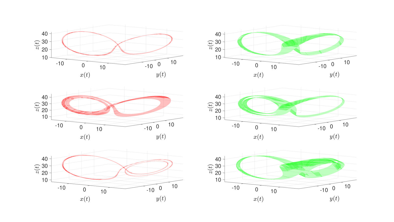
Let $x_{i}$ denote the numerically computed heteroclinic orbits segments illustrated in Figure 5 for the six connecting orbit problems above. Then, the true solutions of (31) have

	$\displaystyle\left\\|x_{I}-\bar{x}_{I}\right\\|_{\infty}<4.0072\cdot 10^{-8},$
	$\displaystyle\left\\|x_{II}-\bar{x}_{II}\right\\|_{\infty}<6.2914\cdot 10^{-8},$
	$\displaystyle\left\\|x_{III}-\bar{x}_{III}\right\\|_{\infty}<1.5951\cdot 10^{-8},$
	$\displaystyle\left\\|x_{IV}-\bar{x}_{IV}\right\\|_{\infty}<5.8614\cdot 10^{-8},$
	$\displaystyle\left\\|x_{V}-\bar{x}_{V}\right\\|_{\infty}<5.8690\cdot 10^{-8},$
	$\displaystyle\left\\|x_{VI}-\bar{x}_{VI}\right\\|_{\infty}<4.7930\cdot 10^{-8}.$

Each connecting orbit segment is computed using $4$ Chebyshev arcs and a uniform meshing of time. Each Chebyshev step is approximated using $100$ modes.

4.2 Cycle-to-cycle connections in Hill’s lunar problem

The following theorem, established using the techniques described above, gives the existence of a transverse heteroclinic cycle in Hill’s Lunar problem (Hill restricted four body problem with $\mu=0$ ) with equal masses, when the Jacobi constant is $2.5$ or $4$ .

Theorem 4.3.

The lunar Hill’s problem admits transverse heteroclinic cycles between the $\mathcal{L}_{1}$ and $\mathcal{L}_{2}$ planar Lyapunov families for both $C=2.5$ and $C=4$ .

Note that there is nothing special about the energy levels $C=2.5$ and $C=4$ . Many similar theorems could be proven using the same methods.

For this theorem, we prove first the existence a pair of periodic orbits in the $\mathcal{L}_{1}$ and $\mathcal{L}_{2}$ Lyapunov families for both $C=2.5$ and $C=4$ . The unstable manifold $P_{\mathcal{L}_{2}}$ , solving Equation (1) is approximated by $\bar{P}_{\mathcal{L}_{2}}$ with $30$ Fourier modes and $4$ Taylor modes, so that

\left\|P_{\mathcal{L}_{2}}-\bar{P}_{\mathcal{L}_{2}}\right\|_{\infty}\leq 1.5175\cdot 10^{-11}.

Similarly, the stable manifold $Q_{\mathcal{L}_{1}}$ , attached to the periodic solution around $\mathcal{L}_{1}$ . We then show that there exists $x_{i}$ , a solution to (31) for each energy level. The connecting orbit segment uses $3$ Chebyshev arcs each approximated using $75$ modes, and satisfying

\displaystyle\left\|x-\bar{x}\right\|_{\infty}<5.0909\cdot 10^{-7}.

The results are illustrated in Figure 6.

A second set of results, proved similarly, are illustrated in Figure 7, for the Hill Restricted Four Body Problem with $\mu=0.00095$ (the Sun-Jupiter value). Here, we prove the existence of transverse heteroclinic connections running both directions between the $\mathcal{L}_{1}$ and $\mathcal{L}_{2}$ planar Lyapunov orbits in the $C=4$ energy level. The non-zero value of $\mu$ breaks the symmetry of the problem, and it is necessary for us to prove both connecting orbits (we cannot infer one from the other). This done, we conclude that there is an asymmetric heteroclinic cycle, and hence chaotic dynamics between the two cycles.

Appendix A A-posteriori analysis: radii polynomials for nonlinear operators between Banach spaces

The goal of the Radii polynomials is to prove that a given operator $T:E\to E$ is a uniform contraction over a subset of $E=E^{(1)}\times\ldots\times E^{(n)}$ , a Banach space. The subset provided by this method is a small ball around the numerical approximation of the solution to the problem $T(x)=x$ . To do so, we have to define $Y$ and $Z$ such as

\displaystyle\left\|(T(\overline{a})-\overline{a})^{(i)}\right\|\leq Y^{(i)}\hskip 14.22636pt

\displaystyle\mbox{and}\hskip 14.22636pt\displaystyle\sup_{b\in B(r)}\left\|\left(DT(\overline{a}+b)\right)^{(i)}\right\|_{\mathcal{B}(E)}\leq Z^{(i)}(r),

(35)

for all $i=1,\ldots,n$ . The norm used in theses bounds will depend on the space $E^{(i)}$ and might not be the same for all $i=1,\ldots,n$ . Appropriates norms will be explicitly shown for every step of the proof in the corresponding sections. The following theorem is using theses bounds to provide the needed result about $T$ .

Theorem A.1.

Let $T$ an operator satisfying the bounds defined in (35) for a given $\overline{a}$ . If
$\left\|Y+Z(r)\right\|_{\infty}<r$ , then for $B:=B_{\overline{a}}(r)$ , we have that $T:B\to B$ is a contraction.

This theorem provides the existence of a fixed point of the operator $T$ considered for the computation of the bounds (35). In order to apply this result, every problem must be written as a Newton like operator. The step to do so depending on the object and the system, it will not be introduced in the general case. Though, it will be explicitly done in every section.
For a given operator well defined on some Banach space $E$ , the bounds (35) can be computed analytically for an arbitrary $r$ . The goal is now to find a way to obtain $r$ such as the theorem is verified. This is why we introduce the radii polynomials.

Definition 5.

Let $Y$ and $Z$ bounds on an operator $T$ as given by (35), we define the Radii polynomials:

p^{(i)}(r):=Y^{(i)}+Z^{(i)}(r)-r,\;i=1,\ldots,n

One can see that the Radii polynomials depend on $Y$ and $Z$ , which are not unique. But the smaller these bounds are, the easier it will be to prove that the operator $T$ is a contraction over a ball around the approximation. The following result will show how the Radii polynomials gives us the value of $r$ for which we can apply theorem (A.1).

Proposition A.2.

Let $T:E\to E$ and $\overline{a}$ an approximation of its fixed point. Consider $p^{(i)}(r)$ , the radii polynomials defined by bounds satisfying (35) and let

\mathcal{I}=\{r>0:p^{(i)}(r)<0,\hskip 8.5359pt\forall i\}.

If $\mathcal{I}\neq\emptyset$ , then $T:B_{\overline{a}}(r)\to B_{\overline{a}}(r)$ is a contraction for every $r\in\mathcal{I}$ .

Proofs and further explanation about the background, and basics examples can be found in [30]. In the the following section, the background will be applied in order to define the radii polynomials granting validation for approximations of the Floquet exponent for a given periodic orbit of the Lorenz system.

Appendix B Some Banach spaces of infinite sequences

Many approximates are done with Fourier series, the coefficients of those series rely in a particular space that we now introduce.

Definition 6.

We denote by $\ell_{\nu}^{1}$ the set of sequences $a=\left(a_{k}\right)_{k\in\mathbb{Z}}$ such as, for some fixed $\nu\geq 1$ , the sum

\sum_{k\in\mathbb{Z}}|a_{k}|\nu^{|k|}=:\left\|a\right\|_{1,\nu}

converges. One can easily see that this sum defines a norm.

Remark B.1.

Let $\nu^{\prime}\geq\nu$ , then

\sum_{k\in\mathbb{Z}}|a_{k}|\nu^{|k|}\leq\sum_{k\in\mathbb{Z}}|a_{k}|\nu^{\prime|k|},

thus if $a\in\ell_{\nu^{\prime}}^{1}$ we have $a\in\ell_{\nu}^{1}$ . Since it is true for every element of $\ell_{\nu^{\prime}}^{1}$ , we have $\ell_{\nu^{\prime}}^{1}\subset\ell_{\nu}^{1}$ . Furthermore, for $a\in\ell_{\nu^{\prime}}^{1}$ , one can easily see from last inequality that we have $\|a\|_{1,\nu}\leq\|a\|_{\nu^{\prime}}$ .

The choice of this space is justified by the fact that it is a Banach algebra under the convolution product. The proof is done in the following lemma.

Lemma B.2.

For $a,b\in\ell_{\nu}^{1}$ , $\left\|a\ast b\right\|_{1,\nu}\leq\left\|a\right\|_{1,\nu}\left\|b\right\|_{1,\nu}$

This approximate will be really useful for approximation including convolution products. For every objects studied in this paper, convolution products of sequences from different spaces will occur, the following remark will be important to understand that the estimates from Lemma B.2 still stand in a slightly modified version.

Remark B.3.

Let $a\in\ell_{\nu}^{1}$ and $b\in\ell_{\nu^{\prime}}^{1}$ . Let $\tilde{\nu}\,\stackrel{{\scriptstyle\mbox{\tiny{\raisebox{0.0pt}[0.0pt][0.0pt]{def}}}}}{{=}}\,\min\{\nu,\nu^{\prime}\}$ , then

\left\|a\ast b\right\|_{\tilde{\nu}}\leq\left\|a\right\|_{\tilde{\nu}}\left\|b\right\|_{\tilde{\nu}}\leq\left\|a\right\|_{1,\nu}\left\|b\right\|_{1,\nu^{\prime}}.

Convolution terms involving coefficients from the previous proof will occur in some of the steps described in this paper. However, different values of $\nu$ might be used for every proof. Thus, in order to make sure that every estimates are valid we must use a smaller value of $\nu$ than the one for the previous proof so we can assume that the estimate is valid in the right space.

Furthermore, the dual space is isometrically isomorphic to a space which is well known and is easy to work with.

Definition 7.

$\ell_{\nu}^{\infty}=\left\{c=\{c_{n}\}_{n\in\mathbb{Z}}:c_{k}\in\mathbb{C},\>\forall k\in\mathbb{Z},\mbox{ and }\left\|c\right\|_{\infty,\frac{1}{\nu}}<\infty\right\}$ , where $\left\|c\right\|_{\infty,\frac{1}{\nu}}=\displaystyle\sup_{n\in\mathbb{Z}}\frac{|c_{n}|}{\nu^{|n|}}$ .

This space is also useful to bound sums such as in the following lemma.

Lemma B.4.

Suppose that $a\in\ell_{\nu}^{1}$ and $c\in\ell_{\nu}^{\infty}$ . then

\left|\sum_{k\in\mathbb{Z}}c_{k}a_{k}\right|\leq\sum_{k\in\mathbb{Z}}|c_{k}||a_{k}|\leq\|c\|_{\infty,\frac{1}{\nu}}\|a\|_{1,\nu}

The proof is straightforward, thus it is left to the reader to verify that this lemma stands. It is useful to get sharp bounds on convolution products when it involves a finite dimension approximation, which can be seen as an element of $\ell_{\nu}^{\infty}$ . The following theorem states that we can study the dual of $\ell_{\nu}^{1}$ spaces through the $\ell_{\nu}^{\infty}$ space. Its proof can be found in [30].

Theorem B.5.

For $\nu\geq 1$ , the space $\ell_{\nu}^{\infty}$ is isometrically isomorphic to $(\ell_{\nu}^{1})^{*}$ .

This result gives us the following equality.

\sup_{\left\|a\right\|_{1,\nu}=1}\left|\sum_{n\in\mathbb{Z}}c_{n}a_{n}\right|=\left\|\ell_{c}\right\|_{(\ell_{\nu}^{1})^{*}}=\left\|c\right\|_{\infty,\frac{1}{\nu}}=\sup_{n\geq 0}\frac{|c_{n}|}{\nu^{n}}.

(36)

Using these kind of sequences will also leads us to infinite operator, whose norm will be evaluated using the following corollary.

Corollary B.6.

Let $A^{(m)}$ a finite matrix of size $2m-1\times 2m-1$ with complex values entries and $\{u_{n}\}_{|n|\geq m}$ a bi-infinite sequence of complex numbers such as $|u_{n}|\leq|u_{m}|$ for every $|n|\geq m$ . Let $a=(a_{k})_{k\in\mathbb{Z}}\in\ell_{\nu}^{1}$ and $a^{(m)}=(a_{-m+1},\ldots,a_{m-1})\in\mathbb{C}^{2m-1}$ its finite dimension projection. Define the linear operator $A$ by

\displaystyle(Aa)_{k}=\begin{cases}(A^{(m)}a^{(m)})_{k},&\mbox{ if }|k|<m\\ u_{k}a_{k},&\mbox{ if }|k|\geq m.\end{cases}

Then $A\in B(\ell_{\nu}^{1},\ell_{\nu}^{1})$ is bounded and

\left\|A\right\|_{B(\ell_{\nu}^{1},\ell_{\nu}^{1})}\leq\max(K,|u_{m}|),

where $K\,\stackrel{{\scriptstyle\mbox{\tiny{\raisebox{0.0pt}[0.0pt][0.0pt]{def}}}}}{{=}}\,\displaystyle\max_{|n|<m}\frac{1}{\nu^{|n|}}\sum_{|k|<m}|A_{k,n}|\nu^{|k|}$ .

The nature of some the objects studied in this work leads to the construction of higher dimensional expansions with one non-periodic direction. We assume again that the series represents an analytic function, which lead to the following definition.

Definition 8.

We denote by $X_{\nu}$ the space of all

x=\left\{x_{\alpha}\in\ell_{\nu}^{1}:\alpha=0,1,2,\ldots\right\}

such that

\|x\|_{X_{\nu}}\,\stackrel{{\scriptstyle\mbox{\tiny{\raisebox{0.0pt}[0.0pt][0.0pt]{def}}}}}{{=}}\,\sum_{\alpha=0}^{\infty}\sum_{k\in\mathbb{Z}}\left|a_{\alpha,k}\right|\nu^{|k|}=\sum_{\alpha=0}^{\infty}\left\|a_{\alpha}\right\|_{1,\nu}<\infty.

An element $x\in X$ will be the result of the expansion of a Taylor series with periodic coefficients, that are themselves expended using a Fourier series. This space also becomes a Banach algebra under the product defined below.

Definition 9.

For $a,b\in X$ , we define the Cauchy-convolution product $\star:X\times X\to X$ by

(a\star b)_{\alpha,k}=\displaystyle\sum_{\begin{subarray}{c}\alpha_{1}+\alpha_{2}=\alpha\\ \alpha_{1},\alpha_{2}\geq 0\end{subarray}}\sum_{\begin{subarray}{c}k_{1}+k_{2}=k\\ k_{1},k_{2}\in\mathbb{Z}\end{subarray}}a_{\alpha_{1},k_{1}}b_{\alpha_{2},k_{2}}.

for all $k\in\mathbb{Z}$ and $\alpha=0,1,2,\ldots$ . The special case where the value $\alpha_{1}=0$ or $\alpha_{2}=0$ are omitted from the sum arise in some circumstances of interested, so that this scenario will be given its own notation $\hat{\star}:X\times X\to X$ . It follows that for all $k\in\mathbb{Z}$ and $\alpha\in\mathbb{Z}^{+}$ , the product is given by

(a\leavevmode\nobreak\ \hat{\star}\leavevmode\nobreak\ b)_{\alpha,k}=\displaystyle\sum_{\begin{subarray}{c}\alpha_{1}+\alpha_{2}=\alpha\\ \alpha_{1},\alpha_{2}>0\end{subarray}}\sum_{\begin{subarray}{c}k_{1}+k_{2}=k\\ k_{1},k_{2}\in\mathbb{Z}\end{subarray}}a_{\alpha_{1},k_{1}}b_{\alpha_{2},k_{2}}.

Appendix C Cauchy Bounds

Lemma C.1 (Bounds for Analytic Functions given by Fourier Series).

Suppose that $\{a_{n}\}_{n\in\mathbb{Z}}$ is a two sided sequence of complex numbers, that $\nu>1$ , that $\omega>0$ , and that

\|a\|_{1,\nu}=\sum_{n\in\mathbb{Z}}|a_{n}|\nu^{|n|}<\infty.

Let

f(z):=\sum_{n\in\mathbb{Z}}a_{n}e^{i\omega kz}.

For $r>0$ let

A_{r}:=\{z\in\mathbb{C}\,|\,|\mbox{{\em imag}}(z)|<r\},

denote the open complex strip of width $r$ .

(1)

$\ell_{\nu}^{1}$ bounds imply $C^{0}$ bounds: The function $f$ is analytic on the strip $A_{r}$ with $r=\ln(\nu)/\omega$ , continuous on the closure of $A_{r}$ , and satisfies

$\sup_{z\in A_{r}}|f(z)|\leq\|a\|_{1,\nu}.$

Moreover $f$ is $T$ -periodic with $T=2\pi/\omega$ .
(II)

Cauchy Bounds: Let $0<\sigma<r$ and

$\tilde{\nu}=e^{\omega(r-\sigma)}.$

Define the sequence $b=\{b_{n}\}_{n\in\mathbb{Z}}$ by

$b_{n}=i\omega na_{n}.$

Then

$\|b\|_{\tilde{\nu}}^{1}\leq\frac{1}{e\sigma}\|a\|_{1,\nu},$

and

$\sup_{z\in A_{r-\sigma}}|f^{\prime}(z)|\leq\frac{1}{e\sigma}\|a\|_{1,\nu}.$

Proof.

For $\nu>1$ , let $r=\ln(\nu)/\omega$ (i.e. $\nu=e^{\omega r}$ ) and consider $z\in A_{r}$ . We have that

$\displaystyle\|f(z)\|$	$\displaystyle\leq$	$\displaystyle\sum_{n\in\mathbb{Z}}\|a_{n}\|\left\|\left(e^{i\omega z}\right)^{n}\right\|$	(37)
	$\displaystyle\leq$	$\displaystyle\sum_{n\in\mathbb{Z}}\|a_{n}\|\left(e^{\omega\left\|\mbox{imag}(z)\right\|}\right)^{\|n\|}$	(38)
	$\displaystyle\leq$	$\displaystyle\sum_{n\in\mathbb{Z}}\|a_{n}\|\nu^{\|n\|}$	(39)
	$\displaystyle=$	$\displaystyle\\|a\\|_{1,\nu}.$	(40)

It follows that $f$ is analytic as the Fourier series converges absolutely and uniformly in $A_{r}$ . Continuity at the boundary of the strip also follows from the absolute summability of the series.

From the fact that $f$ is analytic in $A_{r}$ it follows that the derivative $f^{\prime}(z)$ exists for any $z$ in the interior of $A_{r}$ and that

f^{\prime}(z)=\sum_{n\in\mathbb{Z}}i\omega na_{n}e^{i\omega nz}=\sum_{n\in\mathbb{Z}}b_{n}e^{i\omega nz}.

However the fact that $f$ is uniformly bounded on $A_{r}$ does not imply uniform bounds on $f^{\prime}$ . Indeed it may be that $f^{\prime}$ has singularities at the boundary. In order to obtain uniform bounds on the derivative we give up a portion of the width of the domain. More precisely we consider the supremum of $f^{\prime}$ on the strip $A_{r-\sigma}$ with $0<\sigma<r$ .

First recall that $\nu=e^{\omega r}$ so that $\tilde{\nu}=e^{\omega(r-\sigma)}$ . We now define the function $s\colon\mathbb{R}^{+}\to\mathbb{R}$ by

s(x):=x\alpha^{x},

with $\alpha=\tilde{\nu}/\nu=e^{-\omega\sigma}<1$ . Note that $s(x)\geq 0$ for all $x\geq 0$ , $s(0)=0$ , and that $s(x)\to 0$ as $x\to\infty$ . Moreover $s$ is bounded and attains its maximum at

\hat{x}=\frac{1}{\omega\sigma},

as can be seen by computing the critical point of $s$ . Then we have the bound

s(x)\leq s(\hat{x})=\frac{1}{e\omega\sigma}.

From this we obtain that

$\displaystyle\\|b\\|_{1,tilde\nu}$	$\displaystyle=$	$\displaystyle\sum_{n\in\mathbb{Z}}\|b_{n}\|\tilde{\nu}^{\|n\|}$
	$\displaystyle=$	$\displaystyle\sum_{n\in\mathbb{Z}}\omega\|n\|\|a_{n}\|\tilde{\nu}^{\|n\|}\frac{\nu^{\|n\|}}{\nu^{\|n\|}}$
	$\displaystyle=$	$\displaystyle\sum_{n\in\mathbb{Z}}\omega\|n\|\left(\frac{\tilde{\nu}}{\nu}\right)^{\|n\|}\|a_{n}\|\nu^{\|n\|}$
	$\displaystyle=$	$\displaystyle\sum_{n\in\mathbb{Z}}\omega s(\|n\|)\|a_{n}\|\nu^{\|n\|}$
	$\displaystyle\leq$	$\displaystyle\sum_{n\in\mathbb{Z}}\omega\frac{1}{e\omega\sigma}\|a_{n}\|\nu^{\|n\|}$
	$\displaystyle=$	$\displaystyle\frac{1}{e\sigma}\\|a\\|_{1,\nu}.$

It now follows by $(I)$ that if $z\in A_{r-\sigma}$ then

|f^{\prime}(z)|\leq\|b\|_{1,\tilde{\nu}}\leq\frac{1}{e\sigma}\|a\|_{1,\nu},

as desired. ∎

Lemma C.2 (Bounds for Analytic Functions given by Taylor Series).

Let $\nu>0$ and suppose that $\{a_{n}\}_{n\in\mathbb{N}}$ is a one sided sequence of complex numbers with

\|a\|_{1,\nu}=\sum_{n=0}^{\infty}|a_{n}|\nu^{n}<\infty.

Define

f(z):=\sum_{n=0}^{\infty}a_{n}z^{n},

and let

D_{\nu}:=\{z\in\mathbb{C}\,|\,|z|<\nu\},

denote the complex disk of radius $\nu>0$ centered at the origin.

(1)

$\ell_{\nu}^{1}$ bounds imply $C^{0}$ bounds: The function $f$ is analytic on the disk $D_{\nu}$ , continuous on the closure of $D_{\nu}$ , and satisfies

$\sup_{z\in D_{\nu}}|f(z)|\leq\|a\|_{1,\nu}.$
(II)

Cauchy Bounds: Let $0<\sigma\leq 1$ and

$\tilde{\nu}=\nu e^{-\sigma}.$

Then

$\sup_{z\in D_{\tilde{\nu}}}|f^{\prime}(z)|\leq\frac{1}{\nu\sigma}\|a\|_{1,\nu}.$

Proof.

The proof is similar to the proof of Lemma C.1, the difference being the estimate of the derivative. So, since $f$ is analytic in $D_{\nu}$ we know that

f^{\prime}(z)=\sum_{n=1}^{\infty}na_{n}z^{n-1},

for all $z\in B_{\nu}$ , and again we will trade in some of the domain in order to obtain uniform bounds. To this end choose $0<\sigma\leq 1$ and define $\tilde{\nu}=\nu e^{-\sigma}$ . As in the Fourier case we consider a function $s\colon[0,\infty)\to\mathbb{R}$ defined by

s(x):=xe^{-\sigma x},

and have that $s$ is a positive function with

s(x)\leq\frac{1}{e\sigma}.

Then for any $z\in D_{\tilde{\nu}}$ we have that

$\displaystyle\|f^{\prime}(z)\|$	$\displaystyle=$	$\displaystyle\sum_{n=1}^{\infty}n\|a_{n}\|\|z\|^{n-1}$
	$\displaystyle\leq$	$\displaystyle\sum_{n=1}^{\infty}n\|a_{n}\|\frac{\nu}{\nu}\|\nu e^{-\sigma}\|^{n-1}$
	$\displaystyle\leq$	$\displaystyle\sum_{n=1}^{\infty}\left(\frac{e^{\sigma}}{\nu}ne^{-\sigma n}\right)\|a_{n}\|\nu^{n}$
	$\displaystyle\leq$	$\displaystyle\sum_{n=1}^{\infty}\left(\frac{e}{\nu}ne^{-\sigma n}\right)\|a_{n}\|\nu^{n}$
	$\displaystyle\leq$	$\displaystyle\sum_{n=0}^{\infty}\frac{e}{\nu}s(n)\|a_{n}\|\nu^{n}$
	$\displaystyle\leq$	$\displaystyle\sum_{n=0}^{\infty}\frac{e}{\nu}\frac{1}{e\sigma}\|a_{n}\|\nu^{n}$
	$\displaystyle=$	$\displaystyle\frac{1}{\nu\sigma}\\|a\\|_{1,\nu}^{1}.$

∎

References

[1] D. Ambrosi, G. Arioli, and H. Koch. A homoclinic solution for excitation waves on a contractile substratum. SIAM J. Appl. Dyn. Syst., 11(4):1533–1542, 2012.
[2] Gianni Arioli and Hans Koch. Existence and stability of traveling pulse solutions of the FitzHugh-Nagumo equation. Nonlinear Anal., 113:51–70, 2015.
[3] Joan S. Birman and R. F. Williams. Knotted periodic orbits in dynamical system. II. Knot holders for fibered knots. In Low-dimensional topology (San Francisco, Calif., 1981), volume 20 of Contemp. Math., pages 1–60. Amer. Math. Soc., Providence, RI, 1983.
[4] Joan S. Birman and R. F. Williams. Knotted periodic orbits in dynamical systems. I. Lorenz’s equations. Topology, 22(1):47–82, 1983.
[5] B. Breuer, J. Horák, P. J. McKenna, and M. Plum. A computer-assisted existence and multiplicity proof for travelling waves in a nonlinearly supported beam. J. Differential Equations, 224(1):60–97, 2006.
[6] Jaime Burgos-García and Marian Gidea. Hill’s approximation in a restricted four-body problem. Celestial Mech. Dynam. Astronom., 122(2):117–141, 2015.
[7] Jaime Burgos-García, Jean-Philippe Lessard, and J. D. Mireles James. Spatial periodic orbits in the equilateral circular restricted four-body problem: computer-assisted proofs of existence. Celestial Mech. Dynam. Astronom., 131(1):Paper No. 2, 36, 2019.
[8] Renato Calleja, Carlos García-Azpeitia, Jean-Philippe Lessard, and J. D. Mireles James. Torus knot choreographies in the $n$ -body problem. Nonlinearity, 34(1):313–349, 2021.
[9] Maciej J. Capiński. Computer assisted existence proofs of Lyapunov orbits at $L_{2}$ and transversal intersections of invariant manifolds in the Jupiter-Sun PCR3BP. SIAM J. Appl. Dyn. Syst., 11(4):1723–1753, 2012.
[10] Maciej J. Capiński and Marian Gidea. Arnold diffusion, quantitative estimates, and stochastic behavior in the three-body problem. Comm. Pure Appl. Math., 76(3):616–681, 2023.
[11] Maciej J. Capiński, Shane Kepley, and J. D. Mireles James. Computer assisted proofs for transverse collision and near collision orbits in the restricted three body problem. J. Differential Equations, 366:132–191, 2023.
[12] Roberto Castelli, Jean-Philippe Lessard, and J. D. Mireles James. Parameterization of invariant manifolds for periodic orbits I: Efficient numerics via the Floquet normal form. SIAM J. Appl. Dyn. Syst., 14(1):132–167, 2015.
[13] Roberto Castelli, Jean-Philippe Lessard, and Jason D. Mireles James. Parameterization of invariant manifolds for periodic orbits (II): a posteriori analysis and computer assisted error bounds. J. Dynam. Differential Equations, 30(4):1525–1581, 2018.
[14] S. Day, O. Junge, and K. Mischaikow. A rigorous numerical method for the global analysis of infinite-dimensional discrete dynamical systems. SIAM J. Appl. Dyn. Syst., 3(2):117–160, 2004.
[15] Sarah Day, Yasuaki Hiraoka, Konstantin Mischaikow, and Toshiyuki Ogawa. Rigorous numerics for global dynamics: a study of the Swift-Hohenberg equation. SIAM J. Appl. Dyn. Syst., 4(1):1–31, 2005.
[16] Sarah Day and William D. Kalies. Rigorous computation of the global dynamics of integrodifference equations with smooth nonlinearities. SIAM J. Numer. Anal., 51(6):2957–2983, 2013.
[17] Jean-Pierre Eckmann and Peter Wittwer. A complete proof of the Feigenbaum conjectures. J. Statist. Phys., 46(3-4):455–475, 1987.
[18] Z. Galias and P. Zgliczyński. Computer assisted proof of chaos in the Lorenz equations. Phys. D, 115(3-4):165–188, 1998.
[19] Zbigniew Galias. Positive topological entropy of Chua’s circuit: a computer assisted proof. Internat. J. Bifur. Chaos Appl. Sci. Engrg., 7(2):331–349, 1997.
[20] Zbigniew Galias and Warwick Tucker. Rigorous integration of smooth vector fields around spiral saddles with an application to the cubic Chua’s attractor. J. Differential Equations, 266(5):2408–2434, 2019.
[21] Zbigniew Galias and Piotr Zgliczyński. Chaos in the Lorenz equations for classical parameter values. A computer assisted proof. In Proceedings of the Conference “Topological Methods in Differential Equations and Dynamical Systems” (Kraków-Przegorzały, 1996), number 36, pages 209–210, 1998.
[22] Zbigniew Galias and Piotr Zgliczyński. Abundance of homoclinic and heteroclinic orbits and rigorous bounds for the topological entropy for the Hénon map. Nonlinearity, 14(5):909–932, 2001.
[23] Marcio Gameiro and Jean-Philippe Lessard. Rigorous computation of smooth branches of equilibria for the three dimensional Cahn-Hilliard equation. Numer. Math., 117(4):753–778, 2011.
[24] Javier Gómez-Serrano. Computer-assisted proofs in PDE: a survey. SeMA J., 76(3):459–484, 2019.
[25] John Guckenheimer and R. F. Williams. Structural stability of Lorenz attractors. Inst. Hautes Études Sci. Publ. Math., (50):59–72, 1979.
[26] Antoni Guillamon and Gemma Huguet. A computational and geometric approach to phase resetting curves and surfaces. SIAM J. Appl. Dyn. Syst., 8(3):1005–1042, 2009.
[27] Àlex Haro, Marta Canadell, Jordi-Lluís Figueras, Alejandro Luque, and Josep-Maria Mondelo. The parameterization method for invariant manifolds, volume 195 of Applied Mathematical Sciences. Springer, [Cham], 2016. From rigorous results to effective computations.
[28] Olivier Hénot. On polynomial forms of nonlinear functional differential equations. J. Comput. Dyn., 8(3):309–323, 2021.
[29] Gemma Huguet and Rafael de la Llave. Computation of limit cycles and their isochrons: fast algorithms and their convergence. SIAM J. Appl. Dyn. Syst., 12(4):1763–1802, 2013.
[30] A. Hungria, J.-P. Lessard, and J.D. Mireles-James. Rigorous numerics for analytic solutions of differential equations: the radii polynomial approach. Math. Comp., 2015.
[31] W. Kalies, S. Kepley, and J. Mireles James. Analytic continuation of local (un)stable manifolds with rigorous computer assisted error bounds. SIAM Journal on Applied Dynamical Systems, 17(1):157–202, 2018.
[32] Shane Kepley and J. D. Mireles James. Chaotic motions in the restricted four body problem via Devaney’s saddle-focus homoclinic tangle theorem. J. Differential Equations, 266(4):1709–1755, 2019.
[33] Oscar E. Lanford, III. A computer-assisted proof of the Feigenbaum conjectures. Bull. Amer. Math. Soc. (N.S.), 6(3):427–434, 1982.
[34] Jean-Philippe Lessard and J. D. Mireles James. Computer assisted Fourier analysis in sequence spaces of varying regularity. SIAM J. Math. Anal., 49(1):530–561, 2017.
[35] Jean-Philippe Lessard, J. D. Mireles James, and Julian Ransford. Automatic differentiation for Fourier series and the radii polynomial approach. Phys. D, 334:174–186, 2016.
[36] Jean-Philippe Lessard, Jason D. Mireles James, and Christian Reinhardt. Computer assisted proof of transverse saddle-to-saddle connecting orbits for first order vector fields. J. Dynam. Differential Equations, 26(2):267–313, 2014.
[37] Jean-Philippe Lessard and Christian Reinhardt. Rigorous numerics for nonlinear differential equations using Chebyshev series. SIAM J. Numer. Anal., 52(1):1–22, 2014.
[38] Edward N. Lorenz. Deterministic nonperiodic flow. J. Atmospheric Sci., 20(2):130–141, 1963.
[39] J. D. Mireles James. Fourier-Taylor approximation of unstable manifolds for compact maps: numerical implementation and computer-assisted error bounds. Found. Comput. Math., 17(6):1467–1523, 2017.
[40] J. D. Mireles James. Validated numerics for equilibria of analytic vector fields: invariant manifolds and connecting orbits. In Rigorous numerics in dynamics, volume 74 of Proc. Sympos. Appl. Math., pages 27–80. Amer. Math. Soc., Providence, RI, 2018.
[41] J. D. Mireles James and Maxime Murray. Chebyshev-Taylor parameterization of stable/unstable manifolds for periodic orbits: implementation and applications. Internat. J. Bifur. Chaos Appl. Sci. Engrg., 27(14):1730050, 32, 2017.
[42] Konstantin Mischaikow and Marian Mrozek. Chaos in the Lorenz equations: a computer-assisted proof. Bull. Amer. Math. Soc. (N.S.), 32(1):66–72, 1995.
[43] Konstantin Mischaikow and Marian Mrozek. Chaos in the Lorenz equations: a computer assisted proof. II. Details. Math. Comp., 67(223):1023–1046, 1998.
[44] Konstantin Mischaikow, Marian Mrozek, and Andrzej Szymczak. Chaos in the Lorenz equations: a computer assisted proof. III. Classical parameter values. volume 169, pages 17–56. 2001. Special issue in celebration of Jack K. Hale’s 70th birthday, Part 3 (Atlanta, GA/Lisbon, 1998).
[45] Maxime Murray and J. D. Mireles James. Computer assisted proof of homoclinic chaos in the spatial equilateral restricted four-body problem. J. Differential Equations, 378:559–609, 2024.
[46] Mitsuhiro T. Nakao, Michael Plum, and Yoshitaka Watanabe. Numerical verification methods and computer-assisted proofs for partial differential equations, volume 53 of Springer Series in Computational Mathematics. Springer, Singapore, ©2019.
[47] Mitsuhiro T. Nakao and Nobito Yamamoto. Numerical verifications of solutions for elliptic equations with strong nonlinearity. Numer. Funct. Anal. Optim., 12(5-6):535–543, 1991.
[48] Arnold Neumaier and Thomas Rage. Rigorous chaos verification in discrete dynamical systems. Phys. D, 67(4):327–346, 1993.
[49] Alberto Pérez-Cervera, Tere M-Seara, and Gemma Huguet. A geometric approach to phase response curves and its numerical computation through the parameterization method. J. Nonlinear Sci., 29(6):2877–2910, 2019.
[50] Alberto Pérez-Cervera, Tere M-Seara, and Gemma Huguet. Global phase-amplitude description of oscillatory dynamics via the parameterization method. Chaos, 30(8):083117, 30, 2020.
[51] M. Plum. Computer-assisted existence proofs for two-point boundary value problems. Computing, 46(1):19–34, 1991.
[52] Michael Plum. Verified existence and inclusion results for two-point boundary value problems. In Contributions to computer arithmetic and self-validating numerical methods (Basel, 1989), volume 7 of IMACS Ann. Comput. Appl. Math., pages 341–355. Baltzer, Basel, 1990.
[53] Christian Reinhardt and J. D. Mireles James. Fourier-Taylor parameterization of unstable manifolds for parabolic partial differential equations: formalism, implementation and rigorous validation. Indag. Math. (N.S.), 30(1):39–80, 2019.
[54] S. Smale. Differentiable dynamical systems. Bull. Amer. Math. Soc., 73:747–817, 1967.
[55] Warwick Tucker. The Lorenz attractor exists. C. R. Acad. Sci. Paris Sér. I Math., 328(12):1197–1202, 1999.
[56] Warwick Tucker. A rigorous ODE solver and Smale’s 14th problem. Found. Comput. Math., 2(1):53–117, 2002.
[57] Warwick Tucker. Validated numerics. Princeton University Press, Princeton, NJ, 2011. A short introduction to rigorous computations.
[58] J. B. van den Berg and J.P. Lessard. Rigorous numerics in dynamics. Notices Amer. Math. Soc., 62(9):1057–1061, 2015.
[59] Jan Bouwe van den Berg, Andréa Deschênes, Jean-Philippe Lessard, and Jason D. Mireles James. Stationary coexistence of hexagons and rolls via rigorous computations. SIAM J. Appl. Dyn. Syst., 14(2):942–979, 2015.
[60] Jan Bouwe van den Berg, Andréa Deschênes, Jean-Philippe Lessard, and Jason D. Mireles James. Stationary coexistence of hexagons and rolls via rigorous computations. SIAM Journal on Applied Dynamical Systems, 14(2):942–979, 2015.
[61] Jan Bouwe van den Berg and Jean-Philippe Lessard. Chaotic braided solutions via rigorous numerics: chaos in the Swift-Hohenberg equation. SIAM J. Appl. Dyn. Syst., 7(3):988–1031, 2008.
[62] Jan Bouwe van den Berg and Jean-Philippe Lessard, editors. Rigorous numerics in dynamics, volume 74 of Proceedings of Symposia in Applied Mathematics. American Mathematical Society, Providence, RI, 2018. AMS Short Course: Rigorous Numerics in Dynamics, January 4–5, 2016, Seattle, Washington.
[63] Jan Bouwe van den Berg, J. D. Mireles James, Jean-Philippe Lessard, and Konstantin Mischaikow. Rigorous numerics for symmetric connecting orbits: even homoclinics of the Gray-Scott equation. SIAM J. Math. Anal., 43(4):1557–1594, 2011.
[64] Jan Bouwe van den Berg and Ray Sheombarsing. Rigorous numerics for odes using Chebyshev series and domain decomposition. J. Comput. Dyn., 8(3):353–401, 2021.
[65] J.B. van den Berg, M. Breden, J.-P. Lessard, and M. Murray. Continuation of homoclinic orbits in the suspension bridge equation: a computer-assisted proof. Journal of Differential Equations, 264, 2018.
[66] Yoshitaka Watanabe and Mitsuhiro T. Nakao. Numerical verifications of solutions for nonlinear elliptic equations. Japan J. Indust. Appl. Math., 10(1):165–178, 1993.
[67] Daniel Wilczak. Symmetric heteroclinic connections in the Michelson system: a computer assisted proof. SIAM J. Appl. Dyn. Syst., 4(3):489–514 (electronic), 2005.
[68] Daniel Wilczak. The existence of Shilnikov homoclinic orbits in the Michelson system: a computer assisted proof. Found. Comput. Math., 6(4):495–535, 2006.
[69] Daniel Wilczak. Symmetric homoclinic solutions to the periodic orbits in the Michelson system. Topol. Methods Nonlinear Anal., 28(1):155–170, 2006.
[70] Daniel Wilczak. Uniformly hyperbolic attractor of the Smale-Williams type for a Poincaré map in the Kuznetsov system. SIAM J. Appl. Dyn. Syst., 9(4):1263–1283, 2010. With online multimedia enhancements.
[71] Daniel Wilczak and Piotr Zgliczynski. Heteroclinic connections between periodic orbits in planar restricted circular three-body problem—a computer assisted proof. Comm. Math. Phys., 234(1):37–75, 2003.
[72] Daniel Wilczak and Piotr Zgliczyński. Heteroclinic connections between periodic orbits in planar restricted circular three body problem. II. Comm. Math. Phys., 259(3):561–576, 2005.
[73] Daniel Wilczak and Piotr Zgliczyński. A geometric method for infinite-dimensional chaos: symbolic dynamics for the Kuramoto-Sivashinsky PDE on the line. J. Differential Equations, 269(10):8509–8548, 2020.
[74] R. F. Williams. The structure of Lorenz attractors. In Turbulence Seminar (Univ. Calif., Berkeley, Calif., 1976/1977), volume Vol. 615 of Lecture Notes in Math., pages 94–112. Springer, Berlin-New York, 1977.
[75] Klaudiusz Wójcik and Piotr Zgliczyński. How to show an existence of homoclinic trajectories using topological tools? In International Conference on Differential Equations, Vol. 1, 2 (Berlin, 1999), pages 246–248. World Sci. Publ., River Edge, NJ, 2000.
[76] Piotr Zgliczyński. Fixed point index for iterations of maps, topological horseshoe and chaos. Topol. Methods Nonlinear Anal., 8(1):169–177, 1996.
[77] Piotr Zgliczyński. Rigorous verification of chaos in the Rössler equations. In Scientific computing and validated numerics (Wuppertal, 1995), volume 90 of Math. Res., pages 287–292. Akademie Verlag, Berlin, 1996.
[78] Piotr Zgliczyński. Computer assisted proof of the horseshoe dynamics in the Hénon map. Random Comput. Dynam., 5(1):1–17, 1997.

	$\displaystyle\\|P-P^{N}\\|_{\infty}$	$\displaystyle\leq\sum_{\alpha=0}^{N-1}\\|A_{\alpha}-\bar{A}_{\alpha}\\|_{\infty}+\left\\|\sum_{\alpha=N}^{\infty}A_{\alpha}\right\\|$		(20)
		$\displaystyle\leq r^{N}+\left\\|\sum_{\alpha=N}^{\infty}A_{\alpha}\right\\|.$		(21)

	$\displaystyle\sum_{\alpha=N}^{\infty}\left\\|(a^{1})^{N}\ast(a^{3})^{N}\right\\|_{1,\nu}$	$\displaystyle=\sum_{\alpha=N}^{2N}\left\\|\left([\bar{a}^{1}+e^{1}]\hat{\ast}[\bar{a}^{3}+e^{3}]\right)_{\alpha}\right\\|_{1,\nu}$
		$\displaystyle\leq\sum_{\alpha=N}^{2N}\left\\|(\bar{a}^{1}\hat{\ast}\bar{a}^{3})_{\alpha}\right\\|_{1,\nu}+\left\\|(\bar{a}^{1}\hat{\ast}\bar{e}^{3})_{\alpha}\right\\|_{1,\nu}+\left\\|(\bar{e}^{1}\hat{\ast}\bar{a}^{3})_{\alpha}\right\\|_{1,\nu}+\left\\|(e^{1}\hat{\ast}e^{3})_{\alpha}\right\\|_{1,\nu}$
		$\displaystyle\leq\sum_{\alpha=N}^{2N}\left\\|(\bar{a}^{1}\hat{\ast}\bar{a}^{3})_{\alpha}\right\\|_{1,\nu}+\left\\|(\bar{a}^{1}\hat{\ast}\bar{e}^{3})_{\alpha}\right\\|_{1,\nu}+\left\\|(\bar{e}^{1}\hat{\ast}\bar{a}^{3})_{\alpha}\right\\|_{1,\nu}+\left\\|(e^{1}\hat{\ast}e^{3})_{\alpha}\right\\|_{1,\nu}$
		$\displaystyle\leq r^{N}\left(\left\\|\bar{a}^{1}\right\\|_{X^{N}}+\left\\|\bar{a}^{3}\right\\|_{X^{N}}+r^{N}\right)+\sum_{\alpha=N}^{2N}\left\\|(\bar{a}^{1}\hat{\ast}\bar{a}^{3})_{\alpha}\right\\|_{1,\nu},$

	$\displaystyle\left\\|\left[DR(x)c\right]^{2}\right\\|_{X_{\nu}^{\infty}}$	$\displaystyle=\sum_{\alpha=N}^{\infty}\left\\|\left[((a^{1})^{N}+x^{1})\hat{\ast}c^{3}\right]_{\alpha}+\left[c^{1}\hat{\ast}((a^{3})^{N}+x^{3})\right]_{\alpha}\right\\|_{1,\nu}$
		$\displaystyle\leq\sum_{\alpha=N}^{\infty}\left\\|((a^{1})^{N}\hat{\ast}c^{3})_{\alpha}+(x^{1}\hat{\ast}c^{3})_{\alpha}+(c^{1}\hat{\ast}(a^{3})^{N})_{\alpha}+(c^{1}\hat{\ast}x^{3})_{\alpha}\right\\|_{1,\nu}$
		$\displaystyle\leq\left\\|(a^{1})^{N}\right\\|_{X_{\nu}^{N}}+\left\\|(a^{3})^{N}\right\\|_{X_{\nu}^{N}}+2r,$

	$\displaystyle\left\\|P_{AB}-\bar{P}_{AB}\right\\|_{\infty}<1.2027\cdot 10^{-11},\quad$	$\displaystyle\left\\|Q_{AB}-\bar{Q}_{AB}\right\\|_{\infty}<2.9500\cdot 10^{-10},$
	$\displaystyle\left\\|P_{AAB}-\bar{P}_{AAB}\right\\|_{\infty}<1.1685\cdot 10^{-10},\quad$	$\displaystyle\left\\|Q_{AAB}-\bar{Q}_{AAB}\right\\|_{\infty}<4.0663\cdot 10^{-10},$
	$\displaystyle\left\\|P_{ABB}-\bar{P}_{ABB}\right\\|_{\infty}<5.9731\cdot 10^{-10},\quad$	$\displaystyle\left\\|Q_{ABB}-\bar{Q}_{ABB}\right\\|_{\infty}<1.0012\cdot 10^{-9},$

	$\displaystyle\left\\|x_{I}-\bar{x}_{I}\right\\|_{\infty}<4.0072\cdot 10^{-8},$
	$\displaystyle\left\\|x_{II}-\bar{x}_{II}\right\\|_{\infty}<6.2914\cdot 10^{-8},$
	$\displaystyle\left\\|x_{III}-\bar{x}_{III}\right\\|_{\infty}<1.5951\cdot 10^{-8},$
	$\displaystyle\left\\|x_{IV}-\bar{x}_{IV}\right\\|_{\infty}<5.8614\cdot 10^{-8},$
	$\displaystyle\left\\|x_{V}-\bar{x}_{V}\right\\|_{\infty}<5.8690\cdot 10^{-8},$
	$\displaystyle\left\\|x_{VI}-\bar{x}_{VI}\right\\|_{\infty}<4.7930\cdot 10^{-8}.$

Computer assisted proofs for transverse heteroclinics by the parameterization method

Abstract

1 Introduction

Remark 1.1 (Solving Equation (1)).

Remark 1.2 (Literature on CAP for connecting orbits).

1.1 Two Example Problems

1.1.1 A Dissipative Example: The Lorenz System

1.1.2 A Hamiltonian Example: A Lunar Hill Problem

Remark 1.3 (Polynomial Embedding).

2 Validated numerics for the parameterization method

Example 2.1 (Periodic solutions of the Lorenz system in Fourier space).

Example 2.2 (Periodic solutions of Hill’s three-body problem in Fourier space).

Example 2.3 (Normal bundles in the example system).

Definition 1.

Example 2.4 (The Fourier operator for Taylor coefficients of higher order).

Definition 2.

2.1 Contraction Argument for the tail of the Fourier-Taylor expansion

Definition 3.

Definition 4.

Example 2.5.

Theorem 2.6.

Example 2.7.

Corollary 2.8.

Example 2.9 (The YY and Z​(r)Z(r) bounds).

3 Connections between periodic orbits

Remark 3.1 (Transversality).

Example 3.2 (Connecting orbits in Lorenz).

Remark 3.3 (On the domain decomposition of the Chebyshev Arc).

Remark 3.4 (On the choice of scalar variables).

4 Examples

4.1 Cycle-to-cycle connections in the Lorenz equations

Theorem 4.1.

Theorem 4.2.

4.2 Cycle-to-cycle connections in Hill’s lunar problem

Theorem 4.3.

Appendix A A-posteriori analysis: radii polynomials for nonlinear operators between Banach spaces

Theorem A.1.

Definition 5.

Proposition A.2.

Appendix B Some Banach spaces of infinite sequences

Definition 6.

Remark B.1.

Lemma B.2.

Remark B.3.

Definition 7.

Lemma B.4.

Theorem B.5.

Corollary B.6.

Definition 8.

Definition 9.

Appendix C Cauchy Bounds

Lemma C.1 (Bounds for Analytic Functions given by Fourier Series).

Proof.

Lemma C.2 (Bounds for Analytic Functions given by Taylor Series).

Proof.

References

Computer assisted proofs for transverse heteroclinics
by the parameterization method

Example 2.9 (The $Y$ and $Z(r)$ bounds).