Computer-assisted proofs of “Kariya’s theorem” with computer algebra

Ayane Ito
University of Tsukuba Takefumi Kasai
University of Tsukuba Akira Terui
terui@math.tsukuba.ac.jp
University of Tsukuba

Abstract

We demonstrate computer-assisted proofs of “Kariya’s theorem,” a theorem in elementary geometry, with computer algebra. In the proof of geometry theorem with computer algebra, vertices of geometric figures that are subjects for the proof are expressed as variables. The variables are classified into two classes: arbitrarily given points and the points defined from the former points by constraints. We show proofs of Kariya’s theorem with two formulations according to two ways for giving the arbitrary points: one is called “vertex formulation,” and the other is called “incenter formulation,” with two methods: one is Gröbner basis computation, and the other is Wu’s method. Furthermore, we show computer-assisted proofs of the property that the point so-called “Kariya point” is located on the hyperbola so-called “Feuerbach’s hyperbola”, with two formulations and two methods.

1 Introduction

This paper discusses computer-assisted proofs of “Kariya’s theorem,” a theorem in elementary geometry with computer algebra.

In proving elementary geometry theorems with computer algebra, the hypothesis and the conclusion are expressed as a system of polynomial equations and a polynomial equation, respectively. In this formulation, variables appearing in the equations are divided into two sets: one consists of variables corresponding to arbitrarily given points, and the other one consists of variables corresponding to the points derived from the points represented by the variables in the former set, with constraints. The proof is demonstrated by showing that the algebraic variety defined by “hypothesis” equations is included in the algebraic variety defined by the “conclusion” equation. Generally, the “computation” of the proof is reduced to solving an ideal or a radical membership problem derived from “hypothesis” equations. This computation is accomplished by Gröbner basis computation [4] or Wu’s method [2].

“Kariya’s theorem” [5] is a theorem in elementary geometry related to the incenter of a triangle. It was discovered at the end of the 19th century [1] and is still a subject of study today ([6], [10]). In this paper, we show computational proof of the theorem with two different formulations: 1) with the given points located on the vertices of the triangle (which is called “vertex formulation”), and 2) with the given point located in the vertices of the base and the incenter of the triangle (which is called “incenter formulation”). For each formulation, we show the proof of Kariya’s theorem and its corollary with the methods of Gröbner basis computation and Wu’s method. Furthermore, it is known that the point appearing in the assertion of Kariya’s theorem (so-called “Kariya point”) is located on the rectangle hyperbola called “Feuerbach hyperbola.” Therefore, we also show the computer-assisted proofs of this property with the two formulations above using Gröbner basis computation and Wu’s method. We note that, to the authors’ knowledge, except for the proof of the corollary with incenter formulation (see Section˜2.2.2), the proofs shown in the present paper have never appeared in the literature.

The paper is organized as follows. In Section˜2, Kariya’s theorem and its formulations are shown. In Section˜3, methods of computer-assisted proof of Kariya’s theorem with Gröbner basis computation and Wu’s method are explained. In Section˜4, proofs of Kariya’s theorem with Gröbner basis computation and Wu’s method are demonstrated. In Section˜5, we show proofs of the property that the Kariya point is located on the Feuerbach hyperbola using the two methods with two different formulations. Finally, we make concluding remarks in Section˜6.

2 Kariya’s theorem and its formulations

“Kariya’s theorem” is a theorem in elementary geometry describing a property related to the incenter of a triangle. While several mathematicians have discovered its proof (with generalizations of the original theorem) during the end of the 19th century and the beginning of the 20th century [1], The name of Kariya [5] has remained until today.

Kariya’s theorem is as follows. Note that a claim widely known as “Kariya’s theorem” is a corollary of the following theorem (see Corollary 2).

Theorem 1 (Kariya’s theorem [5])

In triangle $ABC$ , let $O$ be the incenter of the triangle $ABC$ , and let $D^{\prime}$ , $E^{\prime}$ , and $F^{\prime}$ be the points where the incenter circle touches the sides $BC$ , $CA$ , and $AB$ , respectively. For a real number $k$ , let $D$ , $E$ and $F$ be the points on lines $OD^{\prime}$ , $OE^{\prime}$ and $OF^{\prime}$ , respectively, satisfying that $\vv{OD}=k\vv{OD^{\prime}}$ , $\vv{OE}=k\vv{OE^{\prime}}$ , $\vv{OF}=k\vv{OF^{\prime}}$ . Then, the lines $AD$ , $BE$ and $CF$ are concurrent at a point $G$ .

The point $G$ in Theorem 1 is called the “Kariya point.” In Theorem 1, by setting $k=1$ , that is $D$ , $E$ and $F$ coincides with $D^{\prime}$ , $E^{\prime}$ and $F^{\prime}$ , respectively, we obtain the following corollary.

Corollary 2

In triangle $ABC$ , let $D$ , $E$ and $F$ be the points where the incenter circle touches the sides $BC$ , $CA$ and $AB$ , respectively. Then, the lines $AD$ , $BE$ and $CF$ are concurrent at a point $G$ .

In proving a theorem in elementary geometry with computer algebra, we give a coordinate system on the real plane (or space). Then, using the coordinates of the points appearing in the proof as variables, we express the relations on the geometric figures containing those points as algebraic relations of variables, which form polynomial equations. As a result, we express the hypothesis and the conclusion as a system of polynomial equations and a polynomial equation, respectively. As a coordinate system, the cartesian coordinate system is widely used.

Some points appearing in the proof whose coordinates are to be expressed as variables are arbitrarily given, and others are derived from the arbitrarily given points. For the arbitrarily given points, let their coordinates be expressed as $u_{1},u_{2},\dots,u_{m}$ , and the coordinates of the points derived from the arbitrarily given points whose coordinate is expressed with $u_{i}$ be expressed with $x_{1},x_{2},\dots,x_{n}$ . The variables $u_{1},u_{2},\dots,u_{m}$ are called “free variables,” and the variables $x_{1},x_{2},\dots,x_{n}$ are called “dependent variables.”

Properties of geometric figures are expressed as polynomial equations with respect to the above variables. For convenience, tuples of variables are denoted as $\mathbf{u}=(u_{1},u_{2},\dots,u_{m})$ and $\mathbf{x}=(x_{1},x_{2},\dots,x_{n})$ . The number of polynomial equations expressing the hypothesis generally equals the number of dependent variables $m$ . Thus, let the polynomial equations expressing the hypothesis be

h_{1}(\mathbf{u},\mathbf{x})=0,\dots,h_{n}(\mathbf{u},\mathbf{x})=0,

where $h_{1}(\mathbf{u},\mathbf{x}),\dots,h_{n}(\mathbf{u},\mathbf{x})\in\mathbb{R}[\mathbf{u},\mathbf{x}]$ , and the polynomial equation expressing the conclusion be $g(\mathbf{u},\mathbf{x})=0$ , where $g(\mathbf{u},\mathbf{x})\in\mathbb{R}[\mathbf{u},\mathbf{x}]$ .

With the discussion above, let us show formulations of Kariya’s theorem into polynomial equations. We have two kinds of formulations according to setting the arbitrarily given points as

1.

The vertices of triangle $ABC$ , and
2.

The vertices of the base and the incenter of triangle $ABC$ .

The former is called “vertex formulation,” and the latter is called “the incenter formulation.”

2.1 A formulation with setting arbitrarily given points as the vertices of a triangle (vertex formulation)

In vertex formulation, without loss of generality, let $BC$ be the base of triangle $ABC$ with setting $A(u_{1},u_{2})$ , $B(0,0)$ , $C(0,1)$ where $u_{1}>0$ and $u_{2}>0$ . Formulations for Theorem 1 and Corollary 2 are shown as follows.

2.1.1 The case of Theorem 1

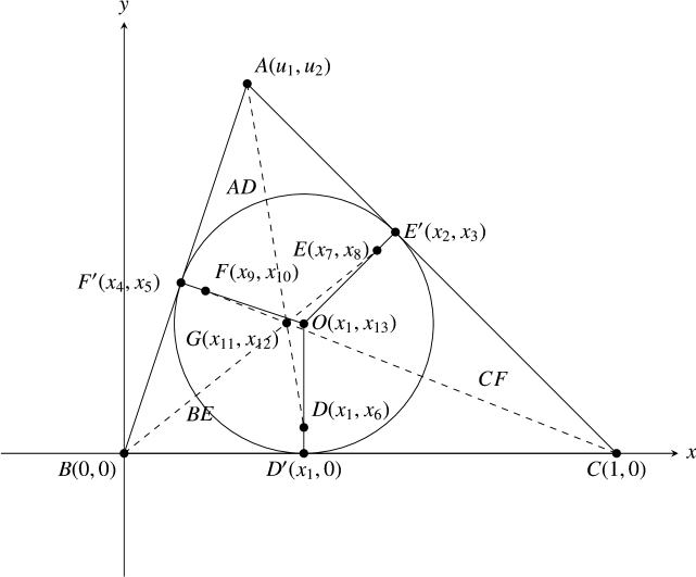
In the formulation of Theorem 1 (see Figure˜1), let $O(x_{1},x_{13})$ be the incenter and $D^{\prime}(x_{1},0)$ , $E^{\prime}(x_{2},x_{3})$ and $F^{\prime}(x_{4},x_{5})$ be the points where the incenter circle touches the sides $BC$ , $CA$ and $AB$ , respectively. Let $D(x_{1},x_{6})$ , $E(x_{7},x_{8})$ and $F(x_{9},x_{10})$ be the points on lines $OD^{\prime}$ , $OE^{\prime}$ and $OF^{\prime}$ , respectively, satisfying that, for $k\in\mathbb{R}$ , $\vv{OD}=k\vv{OD^{\prime}}$ , $\vv{OE}=k\vv{OE^{\prime}}$ and $\vv{OF}=k\vv{OF^{\prime}}$ . Let $G(x_{11},x_{12})$ be the Kariya point. Then, the hypothesis are expressed as $h_{1},\dots,h_{13}$ in Equation˜1, and the conclusion is expressed as $g_{1}$ in Equation˜2. Note that, in each equation, an arrow ( $\Longleftrightarrow$ ) followed by a comment on the right side shows the corresponding geometric condition.

\begin{split}h_{1}&=x_{1}^{2}-x_{4}^{2}-x_{5}^{2}\,\Longleftrightarrow\,BD^{\prime}=BF^{\prime},\\ h_{2}&=(1-x_{1})^{2}-(1-x_{2})^{2}-x_{3}^{2}\,\Longleftrightarrow\,CD^{\prime}=CE^{\prime},\\ h_{3}&=(u_{1}-x_{4})^{2}+(u_{2}-x_{5})^{2}-(u_{1}-x_{2})^{2}-(u_{2}-x_{3})^{2}\,\Longleftrightarrow\,AF^{\prime}=AE^{\prime},\\ h_{4}&=u_{1}x_{5}-u_{2}x_{4}\,\Longleftrightarrow\,\text{$A$, $B$ and $F^{\prime}$ are collinear,}\\ h_{5}&=u_{2}(1-x_{2})-x_{3}(1-u_{1})\,\Longleftrightarrow\,\text{$A$, $E^{\prime}$ and $C$ are collinear,}\\ h_{6}&=(x_{2}-x_{1})^{2}+(x_{3}-x_{13})^{2}-x_{13}^{2}\,\Longleftrightarrow\,OD^{\prime}=OE^{\prime},\\ h_{7}&=(x_{6}-x_{13})+kx_{13}\,\Longleftrightarrow\,\vv{OD}=k\vv{OD^{\prime}},\\ h_{8}&=(x_{7}-x_{1})-k(x_{2}-x_{1})\,\Longleftrightarrow\,\vv{OE}=k\vv{OE^{\prime}}\quad\text{(with respect to the $x$ coordinate),}\\ h_{9}&=(x_{8}-x_{13})-k(x_{3}-x_{13})\,\Longleftrightarrow\,\vv{OE}=k\vv{OE^{\prime}}\quad\text{(with respect to the $y$ coordinate),}\\ h_{10}&=(x_{9}-x_{1})-k(x_{4}-x_{1})\,\Longleftrightarrow\,\vv{OF}=k\vv{OF^{\prime}}\quad\text{(with respect to the $x$ coordinate),}\\ h_{11}&=(x_{10}-x_{13})-k(x_{5}-x_{13})\,\Longleftrightarrow\,\vv{OF}=k\vv{OF^{\prime}}\quad\text{(with respect to the $y$ coordinates),}\\ h_{12}&=(u_{2}-x_{6})(u_{1}-x_{11})-(u_{1}-x_{1})(u_{2}-x_{12})\,\Longleftrightarrow\,\text{$A$, $G$ and $D$ are collinear,}\\ h_{13}&=(1-x_{11})x_{10}-(1-x_{9})x_{12}\,\Longleftrightarrow\,\text{$C$, $G$ and $F$ are collinear.}\end{split}

(1)

g=x_{7}x_{12}-x_{8}x_{11}\,\Longleftrightarrow\,\text{$B$, $G$ and $E$ are collinear.}

(2)

Refer to caption — Fig. 1: An example of Theorem 1 with vertex formulation. See Section˜2.1.1 for details.

2.1.2 The case of Corollary 2

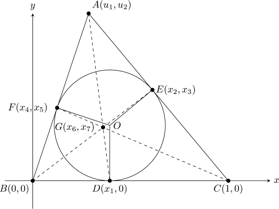
In Corollary 2 (see Figure˜2), the points $D$ , $E$ and $F$ coincides with $D^{\prime}(x_{1},0)$ , $E^{\prime}(x_{2},x_{3})$ and $F^{\prime}(x_{4},x_{5})$ , respectively, in Theorem 1. Thus, in the formulation of Corollary 2, set $D(x_{1},0)$ , $E(x_{2},x_{3})$ , $F(x_{4},x_{5})$ and $G(x_{6},x_{7})$ . Then, the hypothesis are expressed as $h_{1},\dots,h_{8}$ in Equation˜3, and the conclusion is expressed as $g$ in Equation˜4.

\begin{split}h_{1}&=x_{1}^{2}-x_{4}^{2}-x_{5}^{2}\,\Longleftrightarrow\,BD=BF,\\ h_{2}&=(u_{1}-x_{4})^{2}+(u_{2}-x_{5})^{2}-(u_{1}-x_{2})^{2}-(u_{2}-x_{3})^{2}\,\Longleftrightarrow\,AF=AE,\\ h_{3}&=(x_{2}-1)^{2}+x_{3}^{2}-(1-x_{1})^{2}\,\Longleftrightarrow\,CE=CD,\\ h_{4}&=u_{1}x_{5}-u_{2}x_{4}\,\Longleftrightarrow\,\text{$A$, $F$ and $B$ are collinear,}\\ h_{5}&=u_{2}(1-x_{2})-x_{3}(1-u_{1})\,\Longleftrightarrow\,\text{$A$, $E$ and $C$ are collinear,}\\ h_{6}&=(u_{1}-x_{1})x_{7}-(x_{6}-x_{1})u_{2}\,\Longleftrightarrow\,\text{$A$, $G$ and $D$ are collinear,}\\ h_{7}&=x_{2}x_{7}-x_{6}x_{3}\,\Longleftrightarrow\,\text{$B$, $G$ and $E$ are collinear.}\end{split}

(3)

g=(x_{4}-1)x_{7}-(x_{6}-1)x_{5}\,\Longleftrightarrow\,\text{$C$, $G$ and $F$ are collinear.}

(4)

2.2 A formulation with setting arbitrarily given points as the vertices of the base and the incenter of the triangle (incenter formulation)

In incenter formulation, without loss of generality, let $BC$ be the base of triangle $ABC$ with setting $B(0,0)$ and $C(1,0)$ . Furthermore, let $O(u_{1},u_{2})$ be the incenter of triangle $ABC$ . Formulations for Theorem 1 and Corollary 2 are shown as follows.

2.2.1 The case of Theorem 1

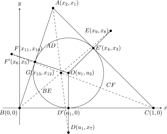
In the formulation of Theorem 1 (see Figure˜3), let $A(x_{2},x_{1})$ be the remaining vertex of the triangle, and let $D^{\prime}(u_{1},0)$ , $E^{\prime}(x_{4},x_{3})$ and $F^{\prime}(x_{6},x_{5})$ be the points where the incenter circle touches the sides $BC$ , $CA$ and $AB$ , respectively. Let $D(u_{1},x_{7})$ , $E(x_{9},x_{8})$ and $F(x_{11},x_{10})$ be the points on the lines $OD^{\prime}$ , $OE^{\prime}$ and $OF^{\prime}$ , respectively, satisfying that, for $k\in\mathbb{R}$ , $\vv{OD}=k\vv{OD^{\prime}}$ , $\vv{OE}=k\vv{OE^{\prime}}$ and $\vv{OF}=k\vv{OF^{\prime}}$ . Then, the hypothesis are expressed as $h_{1},\dots,h_{13}$ in eq.˜5, and the conclusion is expressed as $g_{1}$ in eq.˜6.

\begin{split}h_{1}&=-(u_{1}-1)^{2}x_{1}+u_{2}^{2}x_{1}+2(u_{1}-1)u_{2}(x_{2}-1)\,\Longleftrightarrow\,\tan{\angle BCO}=\tan{\angle OCA},\\ h_{2}&=x_{1}(-u_{1}^{2}+u_{2}^{2})+2u_{1}u_{2}x_{2}\,\Longleftrightarrow\,\tan{\angle CBO}=\tan{\angle OBA},\\ h_{3}&=x_{3}(x_{2}-1)-x_{1}(x_{4}-1)\,\Longleftrightarrow\,\text{$A$, $E^{\prime}$ and $C$ are collinear,}\\ h_{4}&=(x_{2}-1)(x_{4}-u_{1})+x_{1}(x_{3}-u_{2})\,\Longleftrightarrow\,\text{$OE^{\prime}$ and $CA$ intersect perpendicularly,}\\ h_{5}&=x_{1}x_{6}-x_{2}x_{5}\,\Longleftrightarrow\,\text{$A$, $F^{\prime}$ and $B$ are collinear,}\\ h_{6}&=x_{2}(x_{6}-u_{1})+x_{1}(x_{5}-u_{2})\,\Longleftrightarrow\,\text{$OF^{\prime}$ and $BA$ intersect perpendicularly,}\\ h_{7}&=x_{7}+u_{2}(k-1)\,\Longleftrightarrow\,\vv{OD}=k\vv{OD^{\prime}}\,\text{(with respect to the $y$ coordinate),}\\ h_{8}&=(x_{9}-u_{1})-(k(x_{4}-u_{1}))\,\Longleftrightarrow\,\vv{OE}=k\vv{OE^{\prime}}\,\text{(with respect to the $x$ coordinate),}\\ h_{9}&=(x_{8}-u_{2})-(k(x_{3}-u_{2}))\,\Longleftrightarrow\,\vv{OE}=k\vv{OE^{\prime}}\,\text{(with respect to the $y$ coordinate),}\\ h_{10}&=(x_{11}-u_{1})-(k(x_{6}-u_{1}))\,\Longleftrightarrow\,\vv{OF}=k\vv{OF^{\prime}}\,\text{(with respect to the $x$ coordinate),}\\ h_{11}&=(x_{10}-u_{2})-(k(x_{5}-u_{2}))\,\Longleftrightarrow\,\vv{OF}=k\vv{OF^{\prime}}\,\text{(with respect to the $y$ coordinate),}\\ h_{12}&=(x_{13}-u_{1})(x_{1}-x_{7})-(x_{12}-x_{7})(x_{2}-u_{1})\,\Longleftrightarrow\,\text{$A$, $G$ and $D$ are collinear,}\\ h_{13}&=x_{12}(x_{11}-1)-x_{10}(x_{13}-1)\,\Longleftrightarrow\,\text{$C$, $G$ and $F$ are collinear.}\\ \end{split}

(5)

g=x_{8}x_{13}-x_{9}x_{12}\,\Longleftrightarrow\,\text{$B$, $G$ and $E$ are collinear.}

(6)

2.2.2 The case of Corollary 2

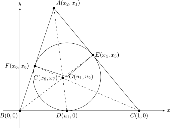
In the formulation of Corollary 2 (see fig.˜4) As in Section˜2.1.2, set $D(u_{1},0)$ , $E(x_{4},x_{3})$ and $F(x_{6},x_{5})$ . Then, the hypothesis are expressed as $h_{1},\dots,h_{7}$ in eq.˜7, and the conclusion is expressed as $g$ in eq.˜8. Note that this formulation has also been given in Chou [2, Example 336].

\begin{split}h_{1}&=u_{2}^{2}((1-x_{4})^{2}+x_{3}^{2})-(1-u_{1})^{2}((u_{1}-x_{4})^{2}+(u_{2}-x_{3})^{2})\,\Longleftrightarrow\,\tan{\angle BCO}=\tan{\angle OCA},\\ h_{2}&=u_{2}^{2}(x_{6}^{2}+x_{5}^{2})-u_{1}^{2}((u_{1}-x_{6})^{2}+(u_{2}-x_{5})^{2})\,\Longleftrightarrow\,\tan{\angle CBO}=\tan{\angle OBA},\\ h_{3}&=x_{3}(x_{2}-1)-x_{1}(x_{4}-1)\,\Longleftrightarrow\,\text{$A$, $E$ and $C$ are collinear,}\\ h_{4}&=x_{3}(x_{3}-u_{2})+(x_{4}-1)(x_{4}-u_{1})\,\Longleftrightarrow\,\text{$OE$ and $CE$ intersect perpendicularly,}\\ h_{5}&=x_{6}x_{1}-x_{2}x_{5}\,\Longleftrightarrow\,\text{$A$, $F$ and $B$ are collinear,}\\ h_{6}&=x_{5}(x_{5}-u_{2})+x_{6}(x_{6}-u_{1})\,\Longleftrightarrow\,\text{$OF$ and $BF$ intersect perpendicularly,}\\ h_{7}&=x_{8}x_{3}-x_{4}x_{7}\,\Longleftrightarrow\,\text{$B$, $G$ and $E$ are collinear,}\\ h_{8}&=(x_{8}-u_{1})x_{1}-x_{7}(x_{2}-u_{1})\,\Longleftrightarrow\,\text{$A$, $G$ and $D$ are collinear.}\end{split}

(7)

g=(x_{8}-1)x_{5}-x_{7}(x_{6}-1)\,\Longleftrightarrow\,\text{$C$, $G$ and $F$ are collinear.}

(8)

3 Proofs of Kariya’s theorem with Gröbner basis computation and Wu’s method

We review the fundamental theory of proving geometric theorem with computer algebra, following Cox et al. [4]. Assume that the hypothesis are expressed as $h_{1}(\mathbf{u},\mathbf{x}),\dots,h_{n}(\mathbf{u},\mathbf{x})$ and the conclusion is expressed as $g(\mathbf{u},\mathbf{x})$ , where $\mathbf{u}$ , $\mathbf{x}$ , $h_{1},\dots,h_{n}$ and $g$ are defined as the same as above. Proving a theorem in elementary geometry can be reduced to showing that the real zeros of the equations a $h_{1}(\mathbf{u},\mathbf{x})=\cdots=h_{n}(\mathbf{u},\mathbf{x})=0$ are also zeros of the equation $g(\mathbf{u},\mathbf{x})=0$ . This idea gives us a naive definition that one can deduce the conclusion. In what follows, let $V=\mathbf{V}(h_{1},\dots,h_{n})\subset\mathbb{R}^{m+n}$ be the affine variety defined by $h_{1},\dots,h_{n}$ and let $\mathbf{I}(V)$ be the ideal of $V$ .

Definition 3 (“follows strictly”)

The conclusion $g$ follows strictly from the hypothesis $h_{1},\dots,h_{n}$ if $g\in\mathbf{I}(V)$ .

Proposition 4

If $g\in\sqrt{\langle{h_{1},\dots,h_{n}}\rangle}$ , then $g$ follows strictly from $h_{1},\dots,h_{n}$ .

From Definition 3 and Proposition 4, a naive proof of the theorem is reduced to solving the radical membership problem. However, this condition seems too strict because the converse of Proposition 4 may not be true. In such a case, there may exist a polynomial $h(\mathbf{u})$ in the hypothesis containing only independent variables $\mathbf{u}$ , and $h(\bar{\mathbf{u}})=0$ for $\bar{\mathbf{u}}=(\bar{u}_{1},\dots,\bar{u}_{m})\in V$ , which means a degenerate case of the configuration of geometric figures [4]. To avoid such degenerate cases, we handle a subvariety of $V$ satisfying that for the points in which a defining polynomial with only independent variables is always nonzero, as in the following definition.

Definition 5 (Algebraically independent)

Let $W\subseteq R^{m+n}$ be an irreducible affine variety with the coordinates $u_{1},\dots,u_{m},x_{1},\dots,x_{n}$ . The variables $u_{1},\dots,u_{m}$ are algebraically independent on $W$ if there exist no nonzero polynomial with variables $u_{1},\dots,u_{m}$ that has zeros in $W$ , that is, $u_{1},\dots,u_{m}$ satisfy that $\mathbf{I}(W)\cap\mathbb{R}[u_{1},\dots,u_{m}]=\{0\}$ .

Then, we accept non-degenerate cases for the geometric proving with the following definition.

Definition 6 (“follows generically”)

The conclusion $g$ follows generically from the hypothesis $h_{1},\dots,h_{n}$ if

g\in\mathbf{I}(V^{\prime})\subseteq R[u_{1},\dots,u_{m},x_{1},\dots,x_{n}],

where $V^{\prime}=W_{1}\cup\cdots\cup W_{p}\subset\mathbb{R}^{m+n}$ satisfying that, for $i=1,\dots,p$ , $W_{i}$ is irreducible and $u_{1},\dots,u_{m}$ are algebraically independent on $W_{i}$ .

Initially, for deriving a proof with Definition 6, one needs to compute irreducible components of $V=\mathbf{V}(h_{1},\dots,h_{n})$ . Fortunately, we have the following proposition.

Proposition 7

Let $H=\langle{h_{1},\dots,h_{n}}\rangle$ . If there exists a nonzero polynomial $c(u_{1},\dots,u_{m})\in\mathbb{R}[u_{1},\dots,u_{m}]$ satisfying that $c\cdot g\in\sqrt{H}$ , then the conclusion $g$ follows generically from the hypothesis $h_{1},\dots,h_{n}$ .

Note that, if $g\in H$ , then $g$ and $H$ satisfy Proposition 7.

3.1 Computing a proof with Gröbner basis computation

This section explains computing a proof with Gröbner basis computation [4]. Proposition 7 tells us that computing a proof is reduced to solving the radical membership problem. We have the following corollary.

Corollary 8

Under the conditions of Proposition 7, the following are equivalent.

1.

There exists a nonzero polynomial $c(u_{1},\dots,u_{m})\in\mathbb{R}[u_{1},\dots,u_{m}]$ satisfying that $c\cdot g\in\sqrt{H}$ .
2.

Let $\tilde{H}$ be an ideal in $\mathbb{R}(u_{1},\dots,u_{m})[x_{1},\dots,x_{n}]$ generated by $h_{1},\dots,h_{n}$ . Then, we have $g\in\sqrt{\tilde{H}}$ .
3.

The reduced Gröbner basis of an ideal $\langle{h_{1},\dots,h_{n},1-yg}\rangle\subseteq\mathbb{R}(u_{1},\dots,u_{m})[x_{1},\dots,x_{n},y]$ is equal to $\{1\}$ .

Corollary 8 tells us that computing the proof is reduced to either solving the ideal membership problem $g\in H$ or computing the reduced Gröber basis of the ideal $\langle{h_{1},\dots,h_{n},1-yg}\rangle$ .

3.2 Computing a proof with Wu’s method

In this section, we explain computing proof with Wu’s method. Note that the method of computation presented here is an elementary version of Wu’s method [4], and a complete version of it can be found in other literature (for example, see Chou [2]). In Wu’s method, we first “triangulate” the polynomials corresponding to the hypothesis by pseudo-divisions. Then, we repeat pseudo-divisions on the polynomial corresponding to the conclusion by the triangulated polynomials to show that the conclusion follows from the hypothesis.

Proposition 9 (Pseudo-division [4])

Let $f,g\in k[x_{1},\ldots,x_{n},y]$ be polynomials expressed as

f=c_{p}y^{p}+\ldots+c_{1}y+c_{0},\quad g=d_{m}y^{m}+\ldots+d_{1}y+d_{0},

(9)

where $c_{i},d_{i}\in k[x_{1},\ldots,x_{n}]$ with $m\leq p$ and $d_{m}\neq 0$ . Then, there exist polynomials $q,r\in k[x_{1},\ldots,x_{n}]$ satisfying the following conditions.

1.

$r=0$ , or $\deg_{y}r<m$ and there exists a nonnegative integer $s$ satisfying $d_{m}^{s}f=qg+r$ .
2.

$r\in\langle{f,g}\rangle$ in the ring $k[x_{1},\ldots,x_{n},y]$ .

In Proposition 9, polynomials $q$ and $r$ are called a pseudoquotient and a pseudoremainder, respectively, of $f$ on pseudo-division by $g$ with respect to $y$ . The pseudoremainder $r$ is denoted by $\mathrm{prem}(f,g,y)$ .

In the algorithm of pseudo-division, $d_{m}^{s}$ is chosen such that the division is executed in the polynomial ring $k[x_{1},\ldots,x_{n}]$ . Furthermore, in place of $d_{m}^{s}$ , $d_{m}/\gcd(d_{m},c_{p},\dots,c_{0})$ can be used for avoiding the growth of degrees of coefficient polynomials [8].

In “triangulation” of the hypothesis polynomials $h_{1},\ldots,h_{n}\in k[\mathbf{u},\mathbf{x}]$ , pseudo-divisions with respect to variables $x_{n},x_{n-1}\ldots,x_{1}$ is executed repeatedly for reducing to a “triangulated” system of polynomials

\begin{split}f_{1}(x_{1}),f_{2}(x_{1},x_{2}),\dots,f_{n}(x_{1},\ldots,x_{n}).\end{split}

(10)

The order of variables used for computing $f_{1},\dots,f_{n}$ is denoted by

x_{n}\succ x_{n-1}\succ\cdots\succ x_{1},

and the set of polynomials in eq.˜10 is called an ascending chain.

Definition 10 (Irreducible ascending chain)

An ascending chain of polynomials in eq.˜10 is called irreducible if, for $i=1,\dots,n$ , $f_{i}$ is irreducible in the polynomial ring $k(u_{1},\dots,u_{m})[x_{i},\dots,x_{i}]/\langle{f_{1},\dots,f_{i-1}}\rangle$ .

Then, for the conclusion polynomial $g\in k[\mathbf{u},\mathbf{x}]$ , pseudo-division by the polynomials in the ascending chain eq.˜10 is repeated for computing polynomials $R_{n-1},\dots,R_{n-0}$ as

R_{n-1}=\mathrm{prem}(g,f_{n},x_{n}),\,R_{n-2}=\mathrm{prem}(R_{n-1},f_{n-1},x_{n-1}),\dots,R_{0}=\mathrm{prem}(R_{1},f_{1},x_{1}),

(11)

and $R_{0}$ is denoted by $\mathrm{prem}(g,f_{1},\dots,f_{n})$ . We have the following proposition.

Proposition 11

Let $\{f_{1},\dots,f_{n}\}$ be an ascending chain derived from the hypothesis polynomials $h_{1},\dots,h_{n}$ expressed as in eq.˜10, and let $g$ be the conclusion polynomial. Then, the following are equivalent.

1.

$\mathrm{prem}(g,f_{1},\dots,f_{n})=0$ .
2.

There exists a nonzero polynomial $c(\mathbf{u})\in\mathbb{R}[\mathbf{u}]$ satisfying that $c\cdot g\in\langle{f_{1},\dots,f_{n}}\rangle$ .

$\mathrm{prem}(g,h_{1},\dots,h_{n})$

In Proposition 11, note that we have $\langle{f_{1},\dots,f_{n}}\rangle\subset H$ , where $H$ is defined as in Proposition 7, since $f_{i}\in H$ . Thus, Corollary 8 and Proposition 11 tells us that, if we have $\mathrm{prem}(g,f_{1},\dots,f_{n})=0$ , then the conclusion $g$ follows generically from the hypothesis $h_{1},\dots,h_{n}$ .

4 Experiments

We have implemented an elementary version of Wu’s method on the Computer Algebra System (CAS) Risa/Asir [7], and have computed proofs of Theorem 1 and Corollary 2 with the Gröbner basis computation and Wu’s method using the vertex and the incenter formulations [9]. The test was conducted in the following environment: Intel Xeon Silver 4210 at 2.20 GHz, RAM 256 GB, Linux 5.4.0 (SMP), Asir Version 20210326.

4.1 Computing proofs with the Gröbner basis computation

This section separately explains computing proofs with the Gröbner basis computation for the vertex and the incenter formulations.

4.1.1 Computing proofs using the vertex formulation

In computing the proof of Theorem 1, for the hypothesis polynomials $h_{1},\dots,h_{13}$ in eq.˜1, we have computed a Grob̈ner basis $G_{1}$ of the ideal $I=\langle{h_{1},\dots,h_{13}}\rangle$ with respect to the degree reverse lexicographic (DegRevLex) ordering with the variable order given as

x_{6}\succ x_{7}\succ x_{8}\succ x_{9}\succ x_{10}\succ x_{11}\succ x_{12}\succ x_{1}\succ x_{2}\succ x_{3}\succ x_{4}\succ x_{5}\succ x_{13}.

(12)

Then, for the conclusion polynomial $g$ in eq.˜2, we have verified that $g\in H=\langle{h_{1},\dots,h_{13}}\rangle$ by showing that the normal form of $g$ with respect to $G_{1}$ is equal to $0$ .

In computing the proof of Corollary 2, for the hypothesis polynomials $h_{1},\dots,h_{7}$ in eq.˜3, we have computed a Grob̈ner basis $G_{2}$ of the ideal $I=\langle{h_{1},\dots,h_{7}}\rangle$ with respect to the DegRevLex ordering with the variable order given as $x_{7}\succ x_{6}\succ x_{5}\succ x_{4}\succ x_{3}\succ x_{2}\succ x_{1}$ . Then, for the conclusion polynomial $g$ in eq.˜4, we have verified that $g\in H=\langle{h_{1},\dots,h_{7}}\rangle$ by showing that the normal form of $g$ with respect to $G_{2}$ is equal to $0$ .

4.1.2 Computing proofs using the incenter formulation

In computing the proof of Theorem 1, for the hypothesis polynomials $h_{1},\dots,h_{13}$ in eq.˜5, we have computed a Grob̈ner basis $G_{3}$ of the ideal $I=\langle{h_{1},\dots,h_{13}}\rangle$ with respect to the DegRevLex ordering with the variable order given as $x_{13}\succ x_{12}\succ x_{11}\succ x_{10}\succ x_{9}\succ x_{8}\succ x_{7}\succ x_{6}\succ x_{5}\succ x_{4}\succ x_{3}\succ x_{2}\succ x_{1}$ . Then, for the conclusion polynomial $g$ in eq.˜6, we have verified that $g\in H=\langle{h_{1},\dots,h_{13}}\rangle$ by showing that the normal form of $g$ with respect to $G_{3}$ is equal to $0$ .

In computing the proof of Corollary 2, for the hypothesis polynomials $h_{1},\dots,h_{7}$ in eq.˜7, we have computed a Grob̈ner basis $G_{4}$ of the ideal $I=\langle{h_{1},\dots,h_{7}}\rangle$ with respect to the DegRevLex ordering with the variable order given as $x_{8}\succ x_{7}\succ x_{6}\succ x_{5}\succ x_{4}\succ x_{3}\succ x_{2}\succ x_{1}$ . We have computed that the normal form of the conclusion polynomial $g$ in eq.˜8 with respect $G_{4}$ is not equal to zero, and the reduced Gröbner basis of the ideal $\langle{h_{1},\dots,h_{7},1-yg}\rangle$ is not equal to $\{1\}$ . Then, by adding a constraint that $u_{1}\neq 0$ (with a new variable $y_{2}$ ), we have computed that the reduced Gröbner basis of the ideal

\langle{h_{1},\dots,h_{7},1-yg,1-y_{2}u_{1}}\rangle

(13)

equals $\{1\}$ .

4.1.3 Computing time and the variable ordering

Table˜1 shows the computing time of computing the proofs in this section. For each formulation, the table shows the computing times of the Gröbner basis and the normal form. The exception is the proof of Corollary 2 using the incenter formulation: in this case, the table shows only the computing time of the reduced Gröbner basis of the ideal in eq.˜13. In the tables below, computing time with the letter ${\dagger}$ , ${\ddagger}$ and ${\dagger}{\dagger}$ denote the average of repeatedly measured data for 10, 100, and 1000 times, respectively.

In each computation of the proof, variable ordering is defined as follows. For the proof of Theorem 1 using the vertex formulation, in the hypothesis polynomials in eq.˜1, the variables $x_{6},x_{7},x_{8},x_{9},x_{10},x_{11},x_{12}$ appear in the terms of total degree $1$ . Thus, we have defined the variable ordering as in eq.˜12 for reducing the terms in $x_{6},x_{7},x_{8},x_{9},x_{10},x_{11},x_{12}$ first. In the other cases, since the computing time of the Gröbner basis, as well as the normal form, was sufficiently small, we have defined the variable ordering as $x_{13}\succ x_{11}\succ\cdots\succ x_{1}$ for the proof of Theorem 1 and $x_{8}\succ x_{7}\succ\cdots\succ x_{1}$ for the proof of Corollary 2.

Table 1: Computing time of the proofs with Gröbner basis computation. Note that computing time with the letter

{\dagger}

, and

{\dagger}{\dagger}

denote the average of repeatedly measured data for 10 and 1000 times, respectively. See Section˜4.1.3 for details.

Formulation	Theorem	Computing time (sec.)
		Gröbner basis	The normal form
Vertex formulation	Theorem 1	$762.0^{{\dagger}}$	$0.4194^{{\dagger}}$
	Corollary 2	$0.524^{{\dagger}}$	$0.02152^{{\dagger}}$
Incenter formulation	Theorem 1	$0.05179^{{\dagger}}$	$0.007314^{{\dagger}}$
	Corollary 2	$0.002069^{{\dagger}{\dagger}}$	N/A

4.2 Computing proofs with Wu’s method

In this section, we explain computing proofs with Wu’s method separately for the vertex and the incenter formulations.

4.2.1 Computing proofs using the vertex formulation

In computing the proof of Theorem 1, we have set the order of variables as

x_{8}\succ x_{7}\succ x_{12}\succ x_{11}\succ x_{10}\succ x_{9}\succ x_{6}\succ x_{13}\succ x_{5}\succ x_{4}\succ x_{3}\succ x_{2}\succ x_{1},

(14)

and, for $h_{1},\dots,h_{13}$ in eq.˜1, computed an ascending chain as

f_{1,1}(x_{1}),f_{1,2}(x_{1},x_{2}),\dots,f_{1,13}(x_{8},x_{7},x_{12},\dots,x_{2},x_{1}).

Then, for $g$ in eq.˜2, we have computed $\mathrm{prem}(g,f_{1,1},\dots,f_{1,13})=0$ .

In computing the proof of Corollary 2, we have set the order of variables as $x_{7}\succ x_{6}\succ x_{5}\succ x_{4}\succ x_{3}\succ x_{2}\succ x_{1}$ , and, for $h_{1},\dots,h_{7}$ in eq.˜3, computed an ascending chain as

f_{2,1}(x_{1}),f_{2,2}(x_{1},x_{2}),\dots,f_{2,7}(x_{7},\dots,x_{2},x_{1}).

Then, for $g$ in eq.˜4, we have computed $\mathrm{prem}(g,f_{2,1},\dots,f_{2,7})=0$ .

4.2.2 Computing proofs using the incenter formulation

In computing the proof of Theorem 1, we have set the order of variables as $x_{13}\succ x_{12}\succ x_{11}\succ x_{10}\succ x_{9}\succ x_{8}\succ x_{7}\succ x_{6}\succ x_{5}\succ x_{4}\succ x_{3}\succ x_{2}\succ x_{1}$ , and, for $h_{1},\dots,h_{13}$ in eq.˜5, computed an ascending chain as

f_{3,1}(x_{1}),f_{3,2}(x_{1},x_{2}),\dots,f_{3,13}(x_{13},x_{12},\dots,x_{2},x_{1}).

Then, for $g$ in eq.˜6, we have computed $\mathrm{prem}(g,f_{3,1},\dots,f_{3,13})=0$ .

In computing the proof of Corollary 2, we have set the order of variables as $x_{8}\succ x_{7}\succ x_{6}\succ x_{5}\succ x_{4}\succ x_{3}\succ x_{2}\succ x_{1}$ , and, for $h_{1},\dots,h_{8}$ in eq.˜7, computed an ascending chain as

f_{4,1}(x_{1}),f_{4,2}(x_{1},x_{2}),\dots,f_{4,8}(x_{8},\dots,x_{2},x_{1}).

Then, for $g$ in eq.˜8, we have computed $\mathrm{prem}(g,f_{4,1},\dots,f_{4,8})=0$ .

4.2.3 Computing time and the variable ordering

Table˜2 shows the computing time of computing this section’s proofs. For each formulation, the table shows the total computing time for calculating the ascending chain and for computing repeated pseudo-divisons of the conclusion polynomial as in eq.˜11.

In each computation of the proof, the order of variables has been defined as follows. For the proof of Theorem 1 using vertex formulation, the conclusion polynomial $g$ in eq.˜2 has variables $x_{7},x_{8},x_{11},x_{12}$ . Furthermore, in the hypothesis polynomials in eq.˜1, there are polynomials with $x_{7}$ and $x_{8}$ of degree 1, respectively. Thus, we have aimed to eliminate $x_{7}$ and $x_{8}$ from $g$ first, then $x_{11}$ and $x_{12}$ from pseudoremainders. After that, since there exist hypothesis polynomials in eq.˜1 which have terms in $x_{11}$ , $x_{10}$ , $x_{9}$ , $x_{6}$ and $x_{13}$ of degree 1, we have aimed to eliminate these variables. As a result, we have defined the order of variables as in eq.˜14. In the other cases, since the computing time was sufficiently short, we have defined the order of variables as $x_{13}\succ x_{12}\succ\cdots\succ x_{1}$ for the proof of Theorem 1 and $x_{8}\succ x_{7}\succ\cdots\succ x_{1}$ for the proof of Corollary 2.

Table 2: Computing time of the proofs with Wu’s method. Note that computing time with the letter

{\dagger}

, and

{\dagger}{\dagger}

denote the average of repeatedly measured data for 10 and 1000 times, respectively. See Section˜4.2.3 for details.

Formulation	Theorem	Computing time (sec.)
Vertex formulation	Theorem 1	$2.952^{{\dagger}}$
	Corollary 2	$0.005355^{{\dagger}{\dagger}}$
Incenter formulation	Theorem 1	$0.00124^{{\dagger}{\dagger}}$
	Corollary 2	$0.01187^{{\dagger}{\dagger}}$

5 Computation on the Feuerbach hyperbola

For a given triangle, the Feuerbach hyperbola is a rectangular hyperbola centered at the point of contact of the nine-point circle and the incircle and passing the triangle’s vertices. Furthermore, it is known that for changing the value of $k$ in Theorem 1, the Kariya point is located on the Feuerbach hyperbola [6]. This section, shows this property with the Gröbner basis computation and Wu’s method using vertex and incenter formulations.

For $a\in\mathbb{R}$ , a rectangular hyperbola whose focus is located at $(\pm\sqrt{2}\,a,0)$ is expressed as

x^{2}-y^{2}=a^{2}.

(15)

By translating the center to $(p_{x},p_{y})$ and rotating $\theta$ counterclockwise, where $p_{x},p_{y},\theta\in\mathbb{R}$ , the hypothesis in eq.˜15 becomes as

(cx+sy-p_{x})^{2}-(-sx+cy-p_{y})^{2}=a^{2},

(16)

where $c=\cos\theta$ , $s=\sin\theta$ .

The proofs are computed as follows. From eq.˜16, let $g^{\prime}=(cx+sy-p_{x})^{2}-(-sx+cy-p_{y})^{2}-a^{2}$ with $x$ and $y$ are replaced with appropriate variables. After computing the Gröbner basis or the ascending set from the hypothesis polynomials in Theorem 1 or Corollary 2, add the constraint $c^{2}+s^{2}-1$ to the Gröbner basis or the ascending set. If the result of the reduction of $g^{\prime}$ by the set of polynomials is equal to $0$ , we see that the Kariya point is located on the Feuerbach hyperbola.

5.1 Computing the proof with Gröbner basis computation

Gröbner basis computation has been used for computing the proofs as follows.

In computing the proof with the vertex formulation, for the Gröbner basis $G_{1}$ computed in Section˜4.1.1, let $\bar{G}_{1}=\{c^{2}+s^{2}-1\}\cup G_{1}$ . Using eq.˜16, let

g^{\prime}=(cx_{11}+sx_{12}-p_{x})^{2}-(-sx_{11}+cx_{12}-p_{y})^{2}-a^{2}\Longleftrightarrow\,\text{$G(x_{11},x_{12})$ is located on the hyperbola},

and we have computed that the normal form of $g^{\prime}$ with respect to $\bar{G}_{1}$ is equal to $0$ to show $g^{\prime}\in\langle{\bar{G}_{1}}\rangle$ .

In computing the proof with the incenter formulation, for the Gröbner basis $G_{3}$ computed in Section˜4.1.2, let $\bar{G}_{3}=\{c^{2}+s^{2}-1\}\cup G_{3}$ . Using eq.˜16, let

g^{\prime}=(cx_{13}+sx_{12}-p_{x})^{2}-(-sx_{13}+cx_{12}-p_{y})^{2}-a^{2}\Longleftrightarrow\,\text{$G(x_{13},x_{12})$ is located on the hyperbola},

and we have computed that the normal form of $g^{\prime}$ with respect to $\bar{G}_{3}$ is equal to $0$ to show $g^{\prime}\in\langle{\bar{G}_{3}}\rangle$ .

5.2 Computing the proof with Wu’s method

Wu’s method has been used for computing the proofs as follows.

In computing the proof with the vertex formulation, for the hypothesis polynomials $h_{1},\dots,h_{9},$ $h_{12},h_{13}$ in eq.˜1, we have computed an ascending chain

f_{5,1}(x_{5}),f_{5,2}(x_{5},x_{13}),\dots,f_{5,11}(x_{5},\dots,x_{8},x_{10}),

with respect to the order of variables given as

x_{10}\succ x_{8}\succ x_{7}\succ x_{6}\succ x_{11}\succ x_{12}\succ x_{1}\succ x_{2}\succ x_{3}\succ x_{4}\succ x_{13}\succ x_{5}.

(17)

Then, let

g^{\prime}=(cx_{11}+sx_{12}-p_{x})^{2}-(-sx_{11}+cx_{12}-p_{y})^{2}-a^{2}\Longleftrightarrow\,\text{$G(x_{11},x_{12})$ is located on the hyperbola},

and we have computed $\mathrm{prem}(g,f_{5,1},\dots,f_{5,11})=0$ .

In computing the proof with the incenter formulation, for a hyperbola in eq.˜15, translate the center to $(p_{x},p_{y})$ and rotate $\theta$ counterclockwise, and let $c=\cos 2\theta$ , $s=\sin 2\theta$ . Let the set of hypothesis polynomials consists of $h_{1},\dots,h_{9},h_{12},g$ in eq.˜5, and

\begin{split}h_{14}&=c^{2}+s^{2}-1\quad\text{(a constraint on $\sin 2\theta$ and $\cos 2\theta$),}\\ h_{15}&=c-2p_{x}c-2p_{y}s\,\Longleftrightarrow\,\text{$B(0,0)$ and $C(1,0)$ are located on the hyperbola,}\\ h_{16}&=x_{2}^{2}c-2x_{2}p_{x}c+2x_{1}x_{2}s-2x_{2}p_{y}s-2p_{x}x_{1}s-x_{1}^{2}c+2x_{1}p_{y}c\\ &\quad\Longleftrightarrow\,\text{$B(0,0)$ and $A(x_{2},x_{1})$ are located on the hyperbola,}\\ h_{17}&=u_{1}^{2}c-2u_{1}p_{x}c+2u_{1}u_{2}s-2u_{1}p_{y}s-2p_{x}u_{2}s-u_{2}^{2}c+2u_{2}p_{y}c\\ &\quad\Longleftrightarrow\,\text{$B(0,0)$ and $O(u1,u2)$ are located on the hyperbola.}\end{split}

(18)

For the set of the hypothesis polynomials, we have computed an ascending chain

f_{6,1}(x_{1}),f_{6,2}(x_{1},x_{2}),\dots,f_{6,15}(x_{1},\dots,p_{y},p_{x}),

with respect to the order of variables as

p_{x}\succ p_{y}\succ c\succ s\succ x_{13}\succ x_{12}\succ x_{9}\succ x_{8}\succ x_{7}\succ x_{6}\succ x_{5}\succ x_{4}\succ x_{3}\succ x_{2}\succ x_{1}.

(19)

Then, let

\begin{split}g^{\prime}&=x_{13}^{2}c-2x_{13}p_{x}c+2x_{13}x_{12}s-2x_{13}p_{y}s-2p_{x}x_{12}s-x_{12}^{2}c+2x_{12}p_{y}c\\ &\quad\Longleftrightarrow\,\text{$B(0,0)$ and $G(x_{13},x_{12})$ are located on the hyperbola},\end{split}

and we have computed $\mathrm{prem}(g_{2},f_{6,1},\dots,f_{6,15})=0$ .

Note that the derivation of $h_{15},h_{16},h_{17},g_{2}$ will be explained in the Appendix.

5.3 Computing time and the variable ordering

Table˜3 shows the computing time of the proofs in this section, with Gröbner basis computation and Wu’s method, using the vertex and the incenter formulations.

The Ordering of variables is defined as follows. In the Gröbner basis computation, the order of variables used for the proof of Theorem 1 are used (see Section˜4.1.3).

In Wu’s method with the vertex formulation, the order of variables are given as in eq.˜17 by the following reason. When we compute the ascending chain, we first eliminate $x_{10}$ because the number of terms in $x_{10}$ which appear in $h_{1},\dots,h_{9},h_{12},h_{13}$ is the smallest among the variables which appear in $h_{1},\dots,h_{9},h_{12},h_{13}$ . Next, we eliminate $x_{8}$ because the number of terms in $x_{8}$ which appear in the input polynomials is the smallest among the variables which appear in the input polynomials. By repeating the procedure, we eliminate the variable in which the number of terms appearing in the polynomials is the smallest in each step in computing the ascending chain.

In Wu’s method with the incenter formulation, the order of variables is given as in eq.˜19 by the following reason. In computing the ascending chain, we first eliminate newly added variables $p_{x}$ , $p_{y}$ , $c$ , and $s$ in this order, then eliminate the rest of the variables with the same ordering as the computation for the proof of Theorem 1 (see Section˜4.2.2).

Table 3: Computing time of the proofs on Feuerbach hyperbola. Note that computing time with the letter

{\dagger}

{\ddagger}

and

{\dagger}{\dagger}

denote the average of repeatedly measured data for 10, 100, and 1000 times, respectively. See Section˜5.3 for details.

Computing method	Formulation	Computing time (sec.)
Gröbner basis	Vertex formulation	$0.01147^{{\dagger}{\dagger}}$
	Incenter formulation	$0.002255^{{\dagger}{\dagger}}$
Wu’s method	Vertex formulation	$0.1639^{{\ddagger}}$
	Incenter formulation	$2.162^{{\dagger}}$

6 Concluding remarks

In this paper, we have demonstrated computational proofs of Kariya’s theorem and its corollary with the Gröbner basis computation and Wu’s method using the vertex and the incenter formulations. Furthermore, we have demonstrated computational proofs of the property that the Kariya point is similarly located on the Feuerbach hyperbola.

Computing time (see Tables˜1 and 2) suggests that the incenter formulation is more suitable for efficient computation for the proof of Theorem 1. For the proof of Corollary 2, while using the incenter formulation made computation more efficient with Gröbner basis computation, using the vertex formulation made computation more efficient with Wu’s method, thus formulation used for better efficiency was different depending on the methods.

Future research topics on computer-assisted proof of Kariya’s theorem with computer algebra include the following.

1.

In Gröbner basis computation and Wu’s method for the proofs, other variable orderings than those used in the present paper may speed up the computation.
2.

Setting the incenter to the origin may speed up the computation using the incenter formulation.
3.

While Kariya’s theorem uses the incenter, the theorem may hold for the excenter(s).
4.

With Gröbner basis computation, the formula of Feuerbach hyperbola may be derived from the hypothesis polynomials.
5.

Although the cartesian coordinate system was used in this paper, other coordinate systems may speed up the computation. (Note that Coanda̧ et al. [3] use the barycentric coordinate system for deriving Kariya’s theorem from their theorem in a more general form.)

Acknowledgements

The research in this paper has been initiated as an undergraduate research project in the College of Mathematics, School of Science and Engineering, University of Tsukuba. The authors thank Nanako Ishii and Gaku Kuriyama for collaborating with the authors during the project.

References

[1] A. Bostan. 11154: Triangle Center X(79), Problems and Solutions. American Mathematics Monthly, 119(8):703–704, October 2012.
[2] S.-C. Chou. Mechanical Geometry Theorem Proving. D. Reidel, 1988.
[3] C. Coanda, F. Smarandache, and I. Patraşcu. A generalization of certain remarkable points of the triangle geometry. In I. Patraşcu and F. Smarandache, editors, Variance of Topics of Plane Geometry, pages 69–73. Education Publishing, 2013.
[4] D. A. Cox, J. Little, and D. O’Shea. Ideals, Varieties, and Algorithms: An Introduction to Computational Algebraic Geometry and Commutative Algebra. Springer, 4th edition, 2015.
[5] J. Kariya. Un theoreme sur le triangle. L’Enseign. Math., 6:130–132, 1904.
[6] S. N. Kiss and P. Yiu. The Touchpoints Triangles and the Feuerbach Hyperbolas. Forum Geometricorum, 14:63–86, 2014.
[7] M. Noro. A computer algebra system: Risa/Asir. In M. Joswig and N. Takayama, editors, Algebra, Geometry and Software Systems, pages 147–162. Springer, 2003.
[8] K. Shiraishi, H. Kai, and M.-T. Noda. Application of stabilized Wu’s method to robot control. In Computer algebra—algorithms, implementations and applications, volume 1295 of RIMS Kôkyûroku, pages 203–208. Kyoto Univ., 2002. (Japanese).
[9] A. Terui, A. Ito, and T. Kasai. teamsnactsukuba/kariya: Pre-submission release (v1.0) [computer software]. Zenodo, 2023. https://doi.org/10.5281/zenodo.7828998
[10] P. Yiu. The Kariya Problem and Related Constructions. Forum Geometricorum, 15:191–201, 2015.

Appendix: Derivation of $h_{15},h_{16},h_{17}$ and $g_{2}$ in Equation˜18

In the appendix, we show derivation of $h_{15},h_{16},h_{17}$ and $g_{2}$ in eq.˜18.

Before deriving the formulas, we show a transform on the hyperbola in eq.˜15. By rotating the hyperbola in eq.˜15 $\theta$ counterclockwise, we have

(x\cos\theta+y\sin\theta)^{2}-(-x\sin\theta+y\cos\theta)^{2}=a^{2}.

Expanding the left-hand side and collecting the terms with respect to $x$ and $y$ is expressed as

x^{2}(\cos^{2}\theta-\sin^{2}\theta)-2xy(2\cos\theta\sin\theta)-y^{2}(\cos^{2}\theta-\sin^{2}\theta)=a^{2}.

By applying the double angle formula, we have

x^{2}c-2xys-y^{2}c=a^{2},

where $c=\cos 2\theta$ , $s=\sin 2\theta$ . By translating the origin to $(p_{x},p_{y})$ , we have

(x-p_{x})^{2}c-2(x-p_{x})(y-p_{y})s-(y-p_{y})^{2}c=a^{2}.

(20)

Now, $h_{15}$ is derived as follows. In Figure˜3, since the hyperbola in eq.˜20 passes through $B(0,0)$ , we have

p_{x}^{2}c-2p_{x}p_{y}s-p_{y}^{2}c=a^{2}.

(21)

Furthermore, since the same hyperbola passes through $C(1,0)$ , we have

(1-p_{x})^{2}c-2(1-p_{x})p_{y}s-p_{y}^{2}c=a^{2}.

(22)

By equating the left-hand-sides of eqs.˜21 and 22, $h_{15}$ is derived.

Next, $h_{16}$ is derived as follows. In Figure˜3, since the hyperbola in eq.˜20 passes through $A(x_{2},x_{1})$ , we have

(x_{2}-p_{x})^{2}c-2(x_{2}-p_{x})(x_{1}-p_{y})s-(x_{1}-p_{y})^{2}c=a^{2}.

(23)

By equating the left-hand-sides of eqs.˜21 and 23, $h_{16}$ is derived.

Next, $h_{17}$ is derived as follows. In Figure˜3, since the hyperbola in eq.˜20 passes through $O(u_{1},u_{2})$ , we have

(u_{1}-p_{x})^{2}c-2(u_{1}-p_{x})(u_{2}-p_{y})s-(u_{2}-p_{y})^{2}c=a^{2}.

(24)

By equating the left-hand-sides of eqs.˜21 and 24, $h_{17}$ is derived.

Finally, $g_{2}$ is derived as follows. In Figure˜3, since the hyperbola in eq.˜20 passes through $G(x_{13},x_{12})$ , we have

(x_{13}-p_{x})^{2}c-2(x_{13}-p_{x})(x_{12}-p_{y})s-(x_{12}-p_{y})^{2}c=a^{2}.

(25)

By equating the left-hand-sides of eqs.˜21 and 25, $g_{2}$ is derived.