Computing finite index congruences of finitely presented semigroups and monoids

Marina Anagnostopoulou-Merkouri, Reinis Cirpons, James D. Mitchell, and Maria Tsalakou

Abstract

In this paper, we describe an algorithm for computing the left, right, or 2-sided congruences of a finitely presented semigroup or monoid with finitely many classes, and an alternative algorithm when the finitely presented semigroup or monoid is finite. We compare the two algorithms presented with existing algorithms and implementations. The first algorithm is a generalization of Sims’ low-index subgroup algorithm for finding the congruences of a monoid. The second algorithm involves determining the distinct principal congruences, and then finding all of their possible joins. Variations of this algorithm have been suggested in numerous contexts by numerous authors. We show how to utilize the theory of relative Green’s relations, and a version of Schreier’s Lemma for monoids, to reduce the number of principal congruences that must be generated as the first step of this approach. Both of the algorithms described in this paper are implemented in the GAP [29] package Semigroups [54], and the first algorithm is available in the C++ library libsemigroups [53] and in its Python bindings libsemigroups_pybind11 [52].

1 Introduction

In this paper, we are concerned with the problem of computing finite index congruences of a finitely presented semigroup or monoid. One case of particular interest is computing the entire lattice of congruences of a finite semigroup or monoid. We will present two algorithms that can perform these computations and compare them with each other and to existing algorithms and their implementations. The first algorithm is the only one of its kind, permitting the computation of finite index 1-sided and 2-sided congruences, and a host of other things (see Section 5) of infinite finitely presented semigroups and monoids. Although this first algorithm is not specifically designed to find finite index subgroups of finitely presented groups, it can be used for such computations and is sometimes faster than the existing implementations in 3Manifolds [15] and GAP [29]; see Table A.5. The second algorithm we present is, for many examples, several orders of magnitude faster than any existing method, and in many cases permits computations that were previously unfeasible. Examples where an implementation of an existing algorithm, such as that in [58], is faster are limited to those with total runtime below 1 second; see Table A.6. Some further highlights include: computing the numbers of right/left congruences of many classical examples of finite transformation and diagram monoids, see Appendix B; reproducing and extending the computations from [6] to find the number of congruences in free semigroups and monoids (see Table B.13); computational experiments with the algorithms implemented were crucial in determining the minimum transformation representation of the so-called diagram monoids in [11]; and in classifying the maximal and minimal 1-sided congruences of the full transformation monoids in [12]. In Appendix A, we present significant quantitative data exhibiting the performance of our algorithms. Appendix B provides a wealth of data generated using the implementation of the algorithms described here. For example, the sequences of numbers of minimal 1-sided congruences of a number of well-studied transformation monoids are apparent in several of the tables in Appendix B, such as Table B.12.

The question of determining the lattice of 2-sided congruences of a semigroup or monoid is classical and has been widely studied in the literature; see, for example, [47]. Somewhat more recently, this interest was rekindled by Araújo, Bentz, and Gomes in [2], Young (né Torpey) in [70], and the third author of the present article, which resulted in [23] and its numerous offshoots [7, 16, 18, 19, 20, 21, 22]. The theory of 2-sided congruences of a monoid is analogous to the theory of normal subgroups of a group, and 2-sided congruences play the same role for monoids with respect to quotients and homomorphisms. As such, it is perhaps not surprising that the theory of 2-sided congruences of semigroups and monoids is rather rich. The 2-sided congruences of certain types of semigroup are completely classified, for a small sample among many, via linked triples for regular Rees 0-matrix semigroups [35, Theorem 3.5.8], or via the kernel and trace for inverse semigroups [35, Section 5.3].

The literature relating to 1-sided congruences is less well-developed; see, for example, [7, 51]. Subgroups are to groups what 1-sided congruences are to semigroups. This accounts, at least in part, for the relative scarcity of results in the literature on 1-sided congruences. The number of such congruences can be enormous, and the structure of the corresponding lattices can be wild. For example, the full transformation monoid of degree $4$ has size $256$ and possesses $22,069,828$ right congruences¹¹1This number was computed for the first time using the algorithm described in Section 4 as implemented in the C++ library libsemigroups [53] whose authors include the authors of the present paper. It was not previously known.. Another example is that of the stylic monoids from [1], which are finite quotients of the well-known plactic monoids [44, 45]. The stylic monoid with $5$ generators has size $51$ , while the number of left congruences is $1,431,795,099$ \@footnotemark.

The purpose of this paper is to provide general computational tools for computing the 1- and 2-sided congruences of a finite, or finitely presented, monoid. There are a number of examples in the literature of such general algorithms; notable examples include [25], [70], and [4], which describes an implementation of the algorithms from [25].

The first of the two algorithms we present is a generalization of Sims’ low-index subgroup algorithm for congruences of a finitely presented monoid; see Section 5.6 in [65] for details of Sims’ algorithm; some related algorithms and applications of the low-index subgroups algorithm can be found in [32], [37], [55, Section 6], and [60]. A somewhat similar algorithm for computing low-index ideals of a finitely presented monoid with decidable word problem was given by Jura in [39] and [40] (see also [61]). We will refer to the algorithm presented here as the low-index congruence algorithm. We present a unified framework for computing various special types of congruences, including: 2-sided congruences; congruences including or excluding given pairs of elements (leading to the ability to compute specific parts of a congruence lattice); solving the word problem in residually finite semigroups or monoids; congruences such that the corresponding quotient is a group; congruences arising from 1- or 2-sided ideals; and 1-sided congruences representing a faithful action of the original monoid; see Section 5 for details. This allows us to, for example, implement a method for computing the finite index ideals of a finitely presented semigroup akin to [39, 40] by implementing a single function (Algorithm 4) which determines if a finite index right congruence is a Rees congruence.

The low-index congruence algorithm takes as input a finite monoid presentation defining a monoid $M$ , and a positive integer $n$ . It permits the congruences with up to $n$ classes to be iterated through without repetition, while only holding a representation of a single such congruence in memory. Each congruence is represented as a certain type of directed graph, which we refer to as word graphs; see Section 2 for the definition. The space complexity of this approach is $O(mn)$ where $m$ is the number of generators of the input monoid, and $n$ is the input positive integer. Roughly speaking, the low-index algorithm performs a backtracking search in a tree whose nodes are word graphs. If the monoid $M$ is finite, then setting $n=|M|$ allows us to determine all of the left, right, or 2-sided congruences of $M$ . Finding all of the subgroups of a finite group was perhaps not the original motivation behind Sims’ low-index subgroup algorithm from [65, Section 5.6]. In particular, there are likely better ways of finding all subgroups of a finite group; see, for example, [33], [36] and the references therein. On the other hand, in some sense, the structure of semigroups and monoids in general is less constrained than that of groups, and in some cases the low-index congruence algorithm is the best or only available means of computing congruences.

To compute the actual lattice of congruences obtained from the low-index congruences algorithm, we require a mechanism for computing the join or meet of two congruences given by word graphs. We show that two well-known algorithms for finite state automata can be used to do this. More specifically, a superficial modification of the Hopcroft-Karp Algorithm [34], for checking if two finite state automata recognise the same language, can be used to compute the join of two congruences. Similarly, a minor modification of the standard construction of an automaton recognising the intersection of two regular languages can be utilised to compute meets; see for example [68, Theorem 1.25]. For more background on automata theory, see [59].

As described in Section 5.6 of [65], one motivation of Sims’ low-index subgroup algorithm was to provide an algorithm for proving non-triviality of the group $G$ defined by a finite group presentation by showing that $G$ has a subgroup of index greater than $1$ . The low-index congruences algorithm presented here can similarly be used to prove the non-triviality of the monoid $M$ defined by a finite monoid presentation by showing that $M$ has a congruence with more than one class. There are a number of other possible applications: to determine small degree transformation representations of monoids (every monoid has a faithful action on the classes of a right congruence); to prove that certain relations in a presentation are irredundant; or more generally to show that the monoids defined by two presentations are not isomorphic (if the monoids defined by $\langle A\mid R\rangle$ and $\langle B\mid S\rangle$ have different numbers of congruences with $n$ classes, then they are not isomorphic). Further applications are discussed in Section 5.

The low-index congruence algorithm is implemented in the open-source C++ library libsemigroups [53], and available for use in the GAP [29] package Semigroups [54], and the Python package libsemigroups_pybind11 [52]. The low-index algorithm is almost embarrassingly parallel, and the implementation in libsemigroups [53] is parallelised using a version of the work stealing queue described in [74, Section 9.1.5]; see Section 4 and Appendix A for more details.

The second algorithm we present is more straightforward than the low-index congruence algorithm, and is a variation on a theme that has been suggested in numerous contexts, for example, in [4, 25, 70]. There are two main steps to this procedure. First, the distinct principal congruences are determined, and, second, all possible joins of the principal congruences are found. Unlike the low-index congruence algorithm, this algorithm cannot be used to compute anything about infinite finitely presented semigroups or monoids. This second algorithm is implemented in the GAP [29] package Semigroups [54].

The first step of the second algorithm, as described in, for example, [4, 25, 70], involves computing the principal congruence, of the input monoid $M$ , generated by every pair $(x,y)\in M\times M$ . Of course, in practice, if $(x,y)\in M\times M$ , then the principal congruences generated by $(x,y)$ and $(y,x)$ are the same, and so only $|M|(|M|-1)/2$ principal congruences are actually generated. In either case, this requires the computation of $O(|M|^{2})$ such principal congruences. We will show that certain of the results from [22] can be generalized to provide a sometimes smaller set of pairs $(x,y)\in M\times M$ required to generate all of the principal congruences of $M$ . In particular, we show how to compute relative Green’s $\mathscr{R}$ -class and $\mathscr{J}$ -class representatives of elements in the direct product $M\times M$ modulo its submonoid $\Delta_{M}=\{\>(m,m)\>:\>m\in M\>\}$ . Relative Green’s relations were introduced in [73]; see also [9, 30]. It is straightforward to verify that if $(x,y),(z,t)\in M\times M$ are $\mathscr{R}$ -related modulo $\Delta_{M}$ , then the principal right congruences generated by $(x,y)$ and $(z,t)$ coincide; see 7.1 i for a proof. We will show that it is possible to reduce the problem of computing relative $\mathscr{R}$ -class representatives to the problems of computing the right action of $\Delta_{M}$ on a set, and membership testing in an associated (permutation) group. The relative $\mathscr{J}$ -class representatives correspond to strongly connected components of the action of $\Delta_{M}$ on the relative $\mathscr{R}$ -classes by left multiplication, and can be found whenever the relative $\mathscr{R}$ -classes can be. In many examples, the time taken to find such relative $\mathscr{R}$ -class and $\mathscr{J}$ -class representatives is negligible when compared to the overall time required to compute the lattice of congruences, and in some examples there is a dramatic reduction in the number of principal congruences that must be generated. For example, if $M$ is the general linear monoid of $3\times 3$ matrices over the finite field $\mathbb{F}_{2}$ of order $2$ , then $|M|=512$ and so $|M|(|M|-1)/2=130,816$ . On the other hand, the numbers of relative $\mathscr{J}$ - and $\mathscr{R}$ -classes of elements of $M\times M$ modulo $\Delta_{M}$ are $44$ and $1,621$ , $M$ has $6$ and $1,621$ principal 2-sided and right congruences, respectively, and the total number of 2-sided congruences is $7$ . Another example: if $N$ is the monoid consisting of all $2\times 2$ matrices over the finite field $\mathbb{F}_{7}$ with $7$ elements with determinant $0$ or $1$ , then $|N|=721$ and so $|N|(|N|-1)/2=259,560$ , but the numbers of relative $\mathscr{J}$ - and $\mathscr{R}$ -classes are $36$ and $1,862$ , there are $7$ and $376$ principal 2-sided and right congruences, respectively, and the total number of 2-sided congruences is $10$ . Of course, there are other examples where there is no reduction in the number of principal congruences that must be generated, and as such the time taken to compute the relative Green’s classes is wasted; see Appendix A for a more thorough analysis.

One question we have not yet addressed is how to compute a (principal) congruence from its generating pairs. For the purpose of computing the lattice of congruences, it suffices to be able to compare congruences by containment. There are a number of different approaches to this: such as the algorithm suggested in [25, Algorithm 2] and implemented in [4], and that suggested in [70, Chapter 2] and implemented in the GAP [29] package Semigroups [54] and the C++ library libsemigroups [53]. The former is essentially a brute force enumeration of the pairs belonging to the congruence, and congruences are represented by the well-known disjoint sets data structure. The latter involves running two instances of the Todd–Coxeter Algorithm in parallel; see [70, Chapter 2] and [13] for more details.

We conclude this introduction with some comments about the relative merits and de-merits of the different approaches outlined above, and we refer the reader to Appendix A for some justification for the claims we are about to make.

As might be expected, the runtime of the low-index congruence algorithm is highly dependent on the input presentation, and it seems difficult (or impossible) to predict what properties of a presentation reduce the runtime. We define the length of a presentation to be the sum of the lengths of the words appearing in relations plus the number of generators. On the one hand, for a fixed monoid $M$ , long presentations appear to have an adverse impact on the performance, but so too do very short presentations. Perhaps one explanation for this is that a long presentation increases the cost of processing each node in the search tree, while a short presentation does not make it evident that certain branches of the tree contain no solutions until many nodes in the tree have been explored. If $M$ is finite, then it is possible to find a presentation for $M$ using, for example, the Froidure-Pin Algorithm [26]. In some examples, the presentations produced mechanically (i.e. non-human presentations) qualify as long in the preceding discussion. In some examples presentations from the literature (i.e. human presentations) work better than their non-human counterparts, but in other examples they qualify as short in the preceding discussion, and are worse. It seems that in many cases some experimentation is required to find a presentation for which the low-index congruence algorithm works best. On the other hand, in examples where the number of congruences is large, say in the millions, running any implementation of the second algorithm is infeasible because it requires too much space. Having said that, there are still some relatively small examples where the low-index congruences algorithm is faster than the implementations of the second algorithm in Semigroups [54] and in CREAM [58], and others where the opposite holds; see Table A.6.

One key difference between the implementation of the low-index subgroup algorithm in, say, GAP [29], and the low-index congruence algorithm in libsemigroups [53] is that the former finds conjugacy class representatives of subgroups with index at most $n\in\mathbb{N}$ . As far as the authors are aware, there is no meaningful notion of conjugacy that can be applied to the low-index congruences algorithm for semigroups and monoids in general. Despite the lack of any optimizations for groups in the implementation of the low-index congruence algorithm in libsemigroups [53], its performance is often better than or comparable to that of the implementations of Sims’ low-index subgroup algorithm in [15] and GAP [29]; see Table A.5 for more details.

The present paper is organised as follows: in Section 2 we present some preliminaries required in the rest of the paper; in Section 3 we state and prove some results related to actions, word graphs, and congruences; in Section 4 we state the low-index congruence algorithm and prove that it is correct; in Section 5 we give numerous applications of the low-index congruences algorithm; in Section 6 we show how to compute the joins and meets of congruences represented by word graphs; in Section 7 we describe the algorithm based on [22] for computing relative Green’s relations. In Appendix A, we provide some benchmarks that compare the performance of the implementations in libsemigroups [53], Semigroups [54], and CREAM [58]. Finally in Appendix B we present some tables containing statistics about the lattices of congruences of some well-known families of monoids.

2 Preliminaries

In this section we introduce some notions that are required for the latter sections of the paper.

Throughout the paper we use the symbol $\bot$ to denote an “undefined” value, and note that $\bot$ is not an element of any set except where it is explicitly included.

Let $S$ be a semigroup. An equivalence relation $\rho\subseteq S\times S$ is a right congruence if $(xs,ys)\in\rho$ for all $(x,y)\in\rho$ and all $s\in S$ . Left congruences are defined analogously, and a 2-sided congruence is both a left and a right congruence. We refer to the number of classes of a congruence as its index.

If $X$ is any set, and $\Psi:X\times S\longrightarrow X$ is a function, then $\Psi$ is a right action of $S$ on $X$ if $((x,s)\Psi,t)\Psi=(x,st)\Psi$ for all $x\in X$ and for all $s,t\in S$ . If in addition $S$ has an identity element $1_{S}$ (i.e. if $S$ is a monoid), we require $(x,1_{S})\Psi=x$ for all $x\in X$ also. Left actions are defined dually. In this paper we will primarily be concerned with right actions of monoids.

If $M$ is a monoid, and $\Psi_{0}:X_{0}\times M\longrightarrow X_{0}$ and $\Psi_{1}:X_{1}\times M\longrightarrow X_{1}$ are right actions of $M$ on sets $X_{0}$ and $X_{1}$ , then we say that $\lambda:X_{0}\longrightarrow X_{1}$ is a homomorphism of the right actions $\Psi_{0}$ and $\Psi_{1}$ if

(x,s)\Psi_{0}\lambda=((x)\lambda,s)\Psi_{1}

for all $x\in X$ and all $s\in M$ . An isomorphism of right actions is a bijective homomorphism.

Let $A$ be any alphabet and let $A^{*}$ denote the free monoid generated by $A$ (consisting of all words over $A$ with operation juxtaposition and identity the empty word $\varepsilon$ ). We define a word graph $\Gamma=(V,E)$ over the alphabet $A$ to be a digraph with set of nodes $V$ and edges $E\subseteq V\times A\times V$ . Word graphs are essentially finite state automata without initial or accept states. More specifically, if $\Gamma=(V,E)$ is a word graph over $A$ , then for any $\alpha\in V$ and any $Q_{1}\subseteq V$ , we can define a finite state automaton $(V,A,\alpha,\delta,Q_{1})$ where: the state set is $V$ ; the alphabet is $A$ ; the start state is $\alpha$ ; the transition function $\delta:V\times A\longrightarrow V$ is defined by $(\alpha,a)\delta=\beta$ whenever $(\alpha,a,\beta)\in E$ ; and $Q_{1}$ denotes the accept states.

If $(\alpha,a,\beta)\in E$ is an edge in a word graph $\Gamma$ , then $\alpha$ is the source, $a$ is the label, and $\beta$ is the target of $(\alpha,a,\beta)$ . A word graph $\Gamma$ is complete if for every node $\alpha$ and every letter $a\in A$ there is at least one edge with source $\alpha$ labelled by $a$ . A word graph $\Gamma=(V,E)$ is finite if the sets of nodes $V$ and edges $E$ are finite. A word graph is deterministic if for every node $\alpha\in V$ and every $a\in A$ there is at most one edge with source $\alpha$ and label $a$ .

If $\alpha,\beta\in V$ , then an $(\alpha,\beta)$ -path is a sequence of edges $(\alpha_{0},a_{0},\alpha_{1}),\ldots,(\alpha_{n-1},a_{n-1},\alpha_{n})\in E$ where $\alpha_{0}=\alpha$ and $\alpha_{n}=\beta$ and $a_{0},\ldots,a_{n-1}\in A$ ; $\alpha$ is the source of the path; the word $a_{0}\cdots a_{n-1}\in A^{*}$ labels the path; $\beta$ is the target of the path; and the length of the path is $n$ . We say that there exists an $(\alpha,\alpha)$ -path of length $0$ labelled by $\varepsilon$ for all $\alpha\in V$ . For $\alpha\in V$ , and $u\in A^{\ast}$ we will write $\alpha\cdot_{\Gamma}u=\beta\in V$ to mean that $u$ labels a $(\alpha,\beta)$ -path in $\Gamma$ , and $\alpha\cdot_{\Gamma}u=\bot$ if $u$ does not label a path with source $\alpha$ in $\Gamma$ . When there are no opportunities for ambiguity we will omit the subscript $\Gamma$ from $\cdot_{\Gamma}$ . If $\alpha,\beta\in V$ and there is an $(\alpha,\beta)$ -path in $\Gamma$ , then we say that $\beta$ is reachable from $\alpha$ . If $\alpha$ is a node in a word graph $\Gamma$ , then the strongly connected component of $\alpha$ is the set of all nodes $\beta$ such that $\beta$ is reachable from $\alpha$ and $\alpha$ is reachable from $\beta$ . If $\Gamma=(V,E)$ is a word graph and $\mathfrak{P}(A^{*}\times A^{*})$ denotes the power set of $A^{*}\times A^{*}$ , then the path relation of $\Gamma$ is the function $\pi_{\Gamma}:V\longrightarrow\mathfrak{P}(A^{*}\times A^{*})$ defined by $(\alpha)\pi_{\Gamma}=\{\>(u,v)\in A^{*}\times A^{*}\>:\>\alpha\cdot u\not=\bot\text{ and }\alpha\cdot u=\alpha\cdot v\>\}$ . If $\Gamma$ is a complete word graph and $\alpha$ is a node in $\Gamma$ , then $(\alpha)\pi_{\Gamma}$ is a right congruence on $A^{*}$ . If $R\subseteq A^{*}\times A^{*}$ , $\Gamma$ is a word graph, and $\pi_{\Gamma}$ is the path relation of $\Gamma$ , then we say that $\Gamma$ is compatible with $R$ if $\alpha\cdot u=\alpha\cdot v$ whenever $\alpha\cdot u\neq\bot$ and $\alpha\cdot v\neq\bot$ for all $(u,v)\in R$ and for all $\alpha\in V$ . Equivalently, if $\Gamma$ is complete, then $\Gamma$ is compatible with $R$ if and only if $R\subseteq(\alpha)\pi_{\Gamma}$ for every node $\alpha$ in $\Gamma$ . It is routine to verify that if a word graph $\Gamma$ is compatible with $R$ , then it is also compatible with the least (2-sided) congruence on $A^{*}$ containing $R$ ; we denote this congruence by $R^{\#}$ .

3 Word graphs and right congruences

In this section we establish some fundamental results related to word graphs and right congruences. It seems likely to the authors that the results presented in this section are well-known; similar ideas occur in [38], [42], [65], and probably elsewhere. However, we did not find any suitable references that suit our purpose here, particularly in Section 3.3, and have included some of the proofs of these results for completeness.

This section has three subsections: in Section 3.1 we describe the relationship between right congruences and word graphs; in Section 3.2 we present some results about homomorphisms between word graphs; and finally in Section 3.3 we give some technical results about standard word graphs.

3.1 Right congruences

Suppose that $M$ is the monoid defined by the monoid presentation $\langle A\mid R\rangle$ and $\Psi:V\times M\longrightarrow V$ is a right action of $M$ on a set $V$ . Recall that $M$ is isomorphic to the quotient of the free monoid $A^{*}$ by $R^{\#}$ . If $\theta:A^{*}\longrightarrow M$ is the surjective homomorphism with $\ker(\theta)=R^{\#}$ , then we can define a complete deterministic word graph $\Gamma=(V,E)$ over the alphabet $A$ such that $(\alpha,a,\beta)\in E$ whenever $(\alpha,(a)\theta)\Psi=\beta$ . Conversely, if $\Gamma=(V,E)$ is a complete word graph that is compatible with $R$ , then we define $\Psi:V\times M\longrightarrow V$ by

(\alpha,(w)\theta)\Psi=\beta

(3.1)

whenever $w$ labels an $(\alpha,\beta)$ -path in $\Gamma$ . It is routine to verify that the functions just described mapping a right action to a word graph, and vice versa, are mutual inverses. For future reference, we record these observations in the next proposition.

Proposition 3.1.

Let $M$ be the monoid defined by the monoid presentation $\langle A\mid R\rangle$ . Then there is a one-to-one correspondence between right actions of $M$ and complete deterministic word graphs over $A$ compatible with $R$ .

If $\Gamma_{0}=(V_{0},E_{0})$ and $\Gamma_{1}=(V_{1},E_{1})$ are word graphs over the same alphabet $A$ , then $\phi:V_{0}\longrightarrow V_{1}$ is a word graph homomorphism if $(\alpha,a,\beta)\in E_{0}$ implies $((\alpha)\phi,a,(\beta)\phi)\in E_{1}$ ; and we write $\phi:\Gamma_{0}\longrightarrow\Gamma_{1}$ . An isomorphism of word graphs $\Gamma_{0}$ and $\Gamma_{1}$ is a bijection $\phi:\Gamma_{0}\longrightarrow\Gamma_{1}$ such that both $\phi$ and $\phi^{-1}$ are homomorphisms. If $\phi:\Gamma_{0}\longrightarrow\Gamma_{1}$ is a word graph homomorphism and $w\in A^{*}$ labels an $(\alpha,\beta)$ -path in $\Gamma_{0}$ , then it is routine to verify that $w$ labels a $((\alpha)\phi,(\beta)\phi)$ -path in $\Gamma_{1}$ .

The correspondence between right actions and word graphs given in 3.1 also preserves isomorphisms, which we record in the next proposition.

Proposition 3.2.

Let $M$ be a monoid generated by a set $A$ , let $\Psi_{0}$ and $\Psi_{1}$ be right actions of $M$ , and let $\Gamma_{0}$ and $\Gamma_{1}$ be the word graphs over $A$ corresponding to these actions. Then $\Psi_{0}$ and $\Psi_{1}$ are isomorphic actions if and only if $\Gamma_{0}$ and $\Gamma_{1}$ are isomorphic word graphs.

Proof.

Assume that $\Gamma_{0}=(V_{0},E_{0})$ and $\Gamma_{1}=(V_{1},E_{1})$ are isomorphic word graphs. Then there exists a bijection $\phi:V_{0}\longrightarrow V_{1}$ . Since $\Gamma_{0}$ and $\Gamma_{1}$ are isomorphic word graphs, $w\in A^{*}$ labels an $(\alpha,\beta)$ -path in $\Gamma_{0}$ if and only if $w$ labels a $((\alpha)\phi,(\beta)\phi)$ -path in $\Gamma_{1}$ . Hence $((\alpha,(w)\theta)\Psi_{0})\phi=((\alpha)\phi,(w)\theta)\Psi_{1}$ for all $\alpha\in V_{0},w\in A^{*}$ and so $\phi$ is an isomorphism of the actions $\Psi_{0}$ and $\Psi_{1}$ .

Conversely, assume that $\Psi_{0}$ and $\Psi_{1}$ are isomorphic right actions of $M$ on sets $V_{0}$ and $V_{1}$ , respectively. Then there exists a bijective homomorphism of right actions $\lambda:V_{0}\longrightarrow V_{1}$ such that $((\alpha,s)\Psi_{0})\lambda=((\alpha)\lambda,s)\Psi_{1}$ for all $\alpha\in V_{0},s\in M$ . We will prove that $\lambda:\Gamma_{0}\longrightarrow\Gamma_{1}$ is a word graph isomorphism. It suffices to show that $(\alpha,a,\beta)\in E_{0}$ if and only if $((\alpha)\lambda,a,(\beta)\lambda)\in E_{1}$ . If $(\alpha,a,\beta)\in E_{0}$ , then $(\alpha,(a)\theta)\Psi_{0}=\beta$ and hence $((\alpha,(a)\theta)\Psi_{0})\lambda=(\beta)\lambda$ . Since $\lambda$ is an isomorphism of right actions $((\alpha,(a)\theta)\Psi_{0})\lambda=((\alpha)\lambda,(a)\theta)\Psi_{1}=(\beta)\lambda$ and so $((\alpha)\lambda,a,(\beta)\lambda)\in E_{1}$ . Similarly, it can be shown that if $((\alpha)\lambda,a,(\beta)\lambda)\in E_{1}$ , then $(\alpha,a,\beta)\in E_{0}$ and hence $\lambda$ defines a word graph isomorphism. ∎

In Section 4 we are concerned with enumerating the right congruences of a monoid $M$ subject to certain restrictions, such as those containing a given set $B\subseteq M\times M$ or those with a given number of equivalence classes. If $M$ is the monoid defined by the presentation $\langle A\mid R\rangle$ and $\rho$ is a right congruence on $M$ , then the function $\Psi:M/\rho\times M\longrightarrow M/\rho$ defined by $(x/\rho,y)\Psi=xy/\rho$ is a right action of $M$ on $M/\rho$ where $x/\rho$ is the equivalence class of $x$ in $\rho$ and $M/\rho=\{\>x/\rho\>:\>x\in M\>\}$ . It follows by 3.1 that $\rho$ corresponds to a complete deterministic word graph $\Gamma$ over $A$ compatible with $R$ . In particular, the nodes of $\Gamma$ are the classes $M/\rho$ , and the edges are $\{(x/\rho,a,(x,a)\Psi):x\in M,\ a\in A\}$ .

On the other hand, not every right action of a monoid is an action on the classes of a right congruence. For example, if $S^{1}$ is a $4\times 4$ rectangular band with an adjoined identity, then two faithful right actions of $S^{1}$ are depicted in Fig. 3.1 with respect to the generating set $\{a:=(1,1),b:=(2,2),c:=(3,3),d:=(4,4)\}\cup\{1_{S^{1}}\}$ . It can be shown that the action of $S^{1}$ on $\{0,\ldots,6\}$ shown in Fig. 3.1 corresponds to a right congruence of $S^{1}$ but that the action of $S^{1}$ on $\{0,\ldots,5\}$ does not.

Figure 3.1: Two faithful right actions of a

4\times 4

rectangular band with identity adjoined; (

a=(1,1)

b=(2,2)

c=(3,3)

d=(4,4)

and for the adjoined identity).

In a word graph $\Gamma$ corresponding to the action of a monoid $M$ on a right congruence $\rho$ , if $m\in M$ , then there exist $a_{0},\ldots,a_{n-1}\in A$ such that $m=a_{0}\cdots a_{n-1}$ , and so $m$ labels the path from $1_{M}$ to $m/\rho$ in $\Gamma$ . In particular, every node in $\Gamma$ is reachable from the node $1_{M}/\rho$ . The converse statement, that every complete deterministic word graph compatible with $R$ where every node is reachable from $1_{M}/\rho$ corresponds to a right congruence on $M$ is established in the next proposition.

If $S$ and $T$ are semigroups, $R\subseteq S\times S$ is a binary relation and $\theta:S\longrightarrow T$ is a homomorphism. Then abusing our notation somewhat we write

(R)\theta=\left\{((u)\theta,(v)\theta)\in T\times T:(u,v)\in R\right\}.

Proposition 3.3.

Let $M$ be the monoid defined by the monoid presentation $\langle A\mid R\rangle$ , let $\theta:A^{*}\longrightarrow M$ be the unique homomorphism with $\ker(\theta)=R^{\#}$ , and let $\Gamma=(V,E)$ be a word graph over $A$ that is complete, deterministic, compatible with $R$ and where every node is reachable from some $\alpha\in V$ . Then $\rho=((\alpha)\pi_{\Gamma})\theta$ is a right congruence on $M$ , where $(\alpha)\pi_{\Gamma}$ is the path relation on $\Gamma$ .

Proof.

Suppose that $((u)\theta,(v)\theta)\in\rho$ for some $(u,v)\in(\alpha)\pi_{\Gamma}$ and that $w\in A^{*}$ is arbitrary. Then $\alpha\cdot u\neq\bot$ and $\alpha\cdot u=\alpha\cdot v$ . Hence $\alpha\cdot uw=(\alpha\cdot u)\cdot w=(\alpha\cdot v)\cdot w=\alpha\cdot vw$ . Since $\Gamma$ is complete, $\alpha\cdot uw\neq\bot$ , and so $(uw,vw)\in(\alpha)\pi_{\Gamma}$ . Therefore $((uw)\theta,(vw)\theta)\in\rho$ , and $\rho$ is a right congruence. ∎

It follows from 3.3 that in order to enumerate the right congruences of $M$ it suffices to enumerate the word graphs over $A$ that are complete, deterministic, compatible with $R$ and where every node is reachable from a node $0$ . Of course, we only want to obtain every right congruence of $S$ once, for which we require the next proposition. Henceforth we will suppose that if $\Gamma=(V,E)$ is a word graph over $A$ , then $V=\{0,\ldots,n-1\}$ for some $n\geq 1$ and so, in particular, $0$ is always a node in $\Gamma$ . Moreover, we will assume that the node $0$ corresponds to the equivalence class $1_{M}/\rho$ of the identity $1_{M}$ of $M$ .

Proposition 3.4.

Let $\Gamma_{0}$ and $\Gamma_{1}$ be word graphs over $A$ corresponding to right congruences of a monoid $M$ generated by $A$ . Then $\Gamma_{0}$ and $\Gamma_{1}$ represent the same right congruence of $M$ if and only if there exists a word graph isomorphism $\phi:\Gamma_{0}\longrightarrow\Gamma_{1}$ such that $(0)\phi=0$ .

Proof.

We denote the right congruences associated to $\Gamma_{0}$ and $\Gamma_{1}$ by $\rho_{0}$ and $\rho_{1}$ , respectively.

Suppose that there exists a word graph isomorphism $\phi:\Gamma_{0}\longrightarrow\Gamma_{1}$ such that $(0)\phi=0$ and that the words $x,y\in A^{*}$ label $(0,\alpha)$ -paths in $\Gamma_{0}$ . Then $x$ and $y$ label $(0,(\alpha)\phi)$ -paths $\Gamma_{1}$ and so $\rho_{0}\subseteq\rho_{1}$ . Since $\phi^{-1}:\Gamma_{1}\longrightarrow\Gamma_{0}$ is a word graph isomorphism satisfying $(0)\phi^{-1}=0$ , it follows that $\rho_{1}\subseteq\rho_{0}$ , and so $\rho_{0}=\rho_{1}$ , as required.

Conversely, assume that $\Gamma_{0}=(V_{0},E_{0})$ and $\Gamma_{1}=(V_{1},E_{1})$ represent the same right congruence of $M$ . We define a word graph homomorphism $\phi:\Gamma_{0}\longrightarrow\Gamma_{1}$ as follows. For every $\alpha\in V_{0}$ , fix a word $w_{\alpha}\in A^{*}$ that labels a $(0,\alpha)$ -path in $\Gamma_{0}$ . We define $(\alpha)\phi$ to be the target of the path with source $0$ labelled by $w_{\alpha}$ in $\Gamma_{1}$ . If $(\alpha,a,\beta)\in E_{0}$ , then both $w_{\alpha}a$ and $w_{\beta}$ label $(0,\beta)$ -paths in $\Gamma_{0}$ , and so $(w_{\alpha}a,w_{\beta})\in(0)\pi_{\Gamma_{0}}=\rho_{0}=\rho_{1}=(0)\pi_{\Gamma_{1}}$ . Hence $((\alpha)\phi,a,(\beta)\phi)$ is an edge of $\Gamma_{1}$ . In addition, $|V_{0}|=|V_{1}|$ and it is clear that if $\alpha\neq\beta$ , then $(\alpha)\phi\neq(\beta)\phi$ and hence $\phi$ is a bijection. ∎

It follows from 3.4 that to enumerate the right congruences of a monoid $M$ defined by the presentation $\langle A\mid R\rangle$ it suffices to enumerate the complete deterministic word graphs over $A$ compatible with $R$ where every node is reachable from 0 up to isomorphism. On the face of it, this is not much of an improvement because, in general, graph isomorphism is a difficult problem. However, word graph isomorphism, in the context of 3.4, is trivial by comparison.

If the alphabet $A=\{a_{0},a_{1},\ldots,a_{n-1}\}$ and $u,v\in A^{*}$ , then we define $u\leq v$ if $|u|<|v|$ or $|u|=|v|$ and $u$ is less than or equal to $v$ in the usual lexicographic order on $A^{*}$ arising from the linear order $a_{0}<a_{1}<\cdots<a_{n-1}$ on $A$ . The order $\leq$ is called the short-lex ordering on $A^{*}$ . If $u\neq v$ and $u\leq v$ , then we write $u<v$ . If $\alpha$ is a node in a word graph $\Gamma$ and $\alpha$ is reachable from $0$ , then there is a $\leq$ -minimum word labelling a $(0,\alpha)$ -path; we denote this path by $w_{\alpha}$ .

The following definition is central to the algorithm presented in Section 4.

Definition 3.5.

A complete word graph $\Gamma=(V,E)$ over $A$ is standard if the following hold:

(i)

$\Gamma$ is deterministic;
(ii)

every node is reachable from $0\in V=\{0,\ldots,|V|-1\}$ ;
(iii)

for all $\alpha,\beta\in V$ , $\alpha<\beta$ if and only if $w_{\alpha}<w_{\beta}$ .

Proposition 3.6.

[cf. Proposition 8.1 in [65]] Let $\Gamma_{0}$ and $\Gamma_{1}$ be standard complete word graphs over the same alphabet. Then there exists a word graph isomorphism $\phi:\Gamma_{0}\longrightarrow\Gamma_{1}$ such that $(0)\phi=0$ if and only if $\Gamma_{0}=\Gamma_{1}$ .

By 3.6, every complete deterministic word graph $\Gamma$ in which every node is reachable from 0 is isomorphic to a unique standard complete word graph. It is straightforward to compute this standard word graph from the original graph by relabelling the nodes, for example, using the procedure SWITCH from [65, Section 4.7]. We refer to this process as standardizing $\Gamma$ .

Another consequence of 3.4 and 3.6 is that enumerating the right congruences of a monoid $M$ defined by a presentation $\langle A\mid R\rangle$ is equivalent to enumerating the standard complete word graphs over $A$ that are compatible with $R$ . As mentioned above, the right action of $M$ on the classes of a right congruence is isomorphic to the right action represented by the corresponding word graph $\Gamma$ . We record this in the following theorem.

Theorem 3.7.

Let $M$ be a monoid defined by a monoid presentation $\langle A\mid R\rangle$ . Then there is a one-to-one correspondence between the right congruences of $M$ and the standard complete word graphs over $A$ compatible with $R$ .

If $\rho$ is a right congruence on $M$ and $\Gamma$ is the corresponding word graph, then the right actions of $M$ on $M/\rho$ and on $\Gamma$ are isomorphic; and $\rho=((0)\pi_{\Gamma})\theta$ where $\theta:A^{*}\longrightarrow M$ is the unique homomorphism with $\ker(\theta)=R^{\#}$ and $(0)\pi_{\Gamma}$ is the path relation on $\Gamma$ .

It is possible to determine a one-to-one correspondence between the right congruences of a semigroup $S$ and certain word graphs arising from $S^{1}$ , as a consequence of 3.7.

Corollary 3.8.

Let $S$ be a semigroup defined by a semigroup presentation $\langle A\mid R\rangle$ . Then there is a one-to-one correspondence between the right congruences of $S$ and the complete word graphs $\Gamma=(V,E)$ for $S^{1}$ over $A$ compatible with $R$ such that $(v,a,0)\not\in E$ for all $v\in V$ and all $a\in A$ .

If $\rho$ is a right congruence of $S$ and $\Gamma$ is the corresponding word graph for $S^{1}$ , then the right actions of $S$ on $S/\rho$ and on $\Gamma\setminus\{0\}$ are isomorphic.

Proof.

By 3.7 it follows that there is a one-to-one correspondence between the right congruences of $S^{1}$ and the complete word graphs $\Gamma=(V,E)$ for $S^{1}$ over $A$ compatible with $R$ . In addition, there is a one-to-one correspondence between the right congruences of $S$ and the right congruences $\rho$ of $S^{1}$ such that $1_{M}/\rho=x/\rho$ if and only if $x=1_{M}$ . Since $\rho$ and $(0)\pi_{\Gamma}$ coincide it follows that there is a one-to-one correspondence between the right congruences $\rho$ of $S^{1}$ such that $1_{M}/\rho=x/\rho$ if and only if $x=1_{M}$ and the complete word graphs $\Gamma=(V,E)$ for $S^{1}$ over $A$ compatible with $R$ such that $(v,a,0)\not\in E$ for all $v\in V$ and all $a\in A$ . The argument to prove that the right actions of $S$ on $S/\rho$ and on $\Gamma\setminus\{0\}$ are isomorphic is identical to the argument in the proof of 3.7. ∎

Given 3.7, we will refer to the standard complete word graph over $A$ compatible with $R$ corresponding to a given right congruence $\rho$ as the word graph of $\rho$ .

We require the following lemma.

Lemma 3.9.

Let $S$ and $T$ be semigroup, let $R\subseteq S\times S$ , and let $\theta:S\longrightarrow T$ be a homomorphism. Then the following hold:

(i)

if $\ker(\theta)\subseteq R$ , $R$ is transitive and $u,v\in S$ are such that $(u)\theta=(u^{\prime})\theta$ and $(v)\theta=(v^{\prime})\theta$ for some $(u^{\prime},v^{\prime})\in R$ , then $(u,v)\in R$ ;
(ii)

if $\theta$ is surjective and $\ker(\theta)$ is contained in the least (left, right, or 2-sided) congruence $\rho$ on $S$ containing $R$ , then the least (left, right, or 2-sided) congruence on $T$ containing $(R)\theta$ is $(\rho)\theta$ .

Lemma 3.9(i) can be reformulated as follows.

Corollary 3.10.

If $\ker(\theta)\subseteq R$ and $R$ is transitive, then $((u)\theta,(v)\theta)\in(R)\theta$ if and only if $(u,v)\in R$ for all $u,v\in S$ .

A convenient consequence of the correspondence between right congruences $\rho$ and their word graphs $\Gamma$ allows us to determine a set of generating pairs for $\rho$ from $\Gamma$ . This method is similar to Stalling’s method for finding a generating set of a subgroup of a free group from its associated coset graph, see, for example, [41, Proposition 6.7].

Lemma 3.11.

Let $M$ be a monoid defined by a monoid presentation $\langle A\mid R\rangle$ , let $\rho$ be a right congruence of $M$ , and let $\Gamma=(V,E)$ be the word graph of $\rho$ . Then $\left\{(w_{\alpha}a,w_{\beta})\in A^{*}\times A^{*}:(\alpha,a,\beta)\in E\right\}$ generates the path relation $(0)\pi_{\Gamma}$ as a right congruence.

In particular, if $\theta:A^{*}\longrightarrow M$ is the natural homomorphism with $\ker(\theta)=R^{\#}$ , then

\left\{((w_{\alpha}a)\theta,(w_{\beta})\theta)\in M\times M:(\alpha,a,\beta)\in E\right\}

generates $\rho$ as a right congruence.

Proof.

We set $W=\{\>w_{\alpha}\>:\>\alpha\in V\>\}$ where $w_{\alpha}$ is the short-lex minimum word labelling any $(0,\alpha)$ -path in $\Gamma$ for every $\alpha\in V$ .

We denote by $\sigma$ the right congruence on $A^{*}$ generated by $S:=\left\{(w_{\alpha}a,w_{\beta})\in A^{*}\times A^{*}:(\alpha,a,\beta)\in E\right\}$ . If $(w_{\alpha}a,w_{\beta})\in S$ , then since $(\alpha,a,\beta)\in E$ , it follows that both $w_{\alpha}a$ and $w_{\beta}$ label $(0,\beta)$ -paths in $\Gamma$ . In particular, $S\subseteq(0)\pi_{\Gamma}$ and so, since $\sigma$ is the least right congruence containing $S$ and $(0)\pi_{\Gamma}$ is a right congruence, $\sigma\subseteq(0)\pi_{\Gamma}$ also.

For the converse inclusion, we will show that $(u,w_{\alpha})\in\sigma$ for every $u\in A^{\ast}$ that labels a $(0,\alpha)$ -path in $\Gamma$ . It will follow from this that $(0)\pi_{\Gamma}\subseteq\sigma$ .

Suppose that $u\in A^{\ast}$ labels a $(0,\alpha)$ -path in $\Gamma$ . We write $u=w_{\beta}v$ where $w_{\beta}$ is the longest prefix of $u$ belonging to $W$ . We proceed by induction on $|v|$ . If $|v|=0$ , then $u=w_{\beta}$ , and so $\beta=\alpha$ . Hence $u=w_{\alpha}$ and so $(u,w_{\alpha})\in\sigma$ by reflexivity. This establishes the base case.

Suppose that for some $k\geq 0$ , $(u,w_{\alpha})\in\sigma$ for all $u\in A^{*}$ such that $u$ labels a $(0,\alpha)$ -path and $u=w_{\beta}v$ where $|v|\leq k$ . Let $u=w_{\beta}v$ for some $v\in A^{*}$ with $|v|=k+1>0$ . Then we may write $v=av_{0}$ for some $a\in A$ and $v_{0}\in A^{\ast}$ with $|v_{0}|=k$ . Since $\Gamma$ is complete, there is an edge $(\beta,a,\gamma)\in E$ for some $\gamma\in V$ . Hence $(w_{\beta}a,w_{\gamma})\in S$ by definition.

If we set $u_{0}=w_{\gamma}v_{0}$ , then $u_{0}$ also labels a $(0,\alpha)$ -path in $\Gamma$ . Again we write $u_{0}=w_{\delta}v_{1}$ where $w_{\delta}$ is the maximal prefix of $u_{0}$ in $W$ and $v_{1}\in A^{*}$ . Since $w_{\gamma}$ is a prefix of $u_{0}$ and $w_{\delta}$ is maximal, $w_{\gamma}$ is a (not necessarily proper) prefix of $w_{\delta}$ . In particular, $|w_{\delta}|\geq|w_{\gamma}|$ and so $|v_{1}|\leq|v_{0}|=k$ . Hence by induction $(u_{0},w_{\alpha})\in\sigma$ . In addition $(u,u_{0})=(w_{\beta}av_{0},w_{\gamma}v_{0})\in\sigma$ , since $(w_{\beta}a,w_{\gamma})\in S\subseteq\sigma$ and $\sigma$ is a right congruence. Therefore by transitivity $(u,w_{\alpha})\in\sigma$ , as required.

Since $R^{\#}=\ker(\theta)\subseteq(0)\pi_{\Gamma}=\sigma$ (we have that $R^{\#}\subseteq(0)\pi_{\Gamma}$ since $\Gamma$ is complete and compatible with $R$ ), we can apply Lemma 3.9 ii to show that $(S)\theta=\left\{((w_{\alpha}a)\theta,(w_{\beta})\theta)\in M\times M:(\alpha,a,\beta)\in E\right\}$ generates $\rho$ as a right congruence. It follows that $(\sigma)\theta=((0)\pi_{\Gamma})\theta=\rho$ is generated by $(S)\theta$ . ∎

From this point in the paper onwards, for the purposes of describing the time or space complexity of some claims, we assume that we are using the RAM model of computation. The following corollary is probably well-known.

Corollary 3.12.

Let $M$ be a monoid defined by a monoid presentation $\langle A\mid R\rangle$ , and let $\rho$ be a right congruence on $M$ . If $\rho$ has finite index $n\in\mathbb{N}$ , then $\rho$ is finitely generated as a right congruence and a set of generating pairs for $\rho$ can be determined in $O(n^{2}|A|)$ time from the word graph associated to $\rho$ .

Proof.

This follows immediately since the generating set for $\rho$ given in Lemma 3.11 has size $n|A|$ , and it can be found by a breadth first traversal of the word graph. The breadth first traversal of the word graph has time complexity $O(n|A|)$ . To store the generating pairs $(u,v)\in A^{*}\times A^{*}$ for $\rho$ requires at most $O(n^{2}|A|)$ space and time, yielding the stated time complexity. ∎

3.2 Homomorphisms of word graphs

In this section we state some results relating homomorphisms of word graphs and containment of the associated congruences.

Lemma 3.13.

If $\Gamma_{0}=(V_{0},E_{0})$ and $\Gamma_{1}=(V_{1},E_{1})$ are deterministic word graphs on the same alphabet $A$ such that every node in $\Gamma_{0}$ and $\Gamma_{1}$ is reachable from $0\in V_{0}$ and $0\in V_{1}$ , respectively, then there exists at most one word graph homomorphism $\phi:\Gamma_{0}\longrightarrow\Gamma_{1}$ such that $(0)\phi=0$ .

Proof.

Suppose that $\phi_{0},\phi_{1}:\Gamma_{0}\longrightarrow\Gamma_{1}$ are word graph homomorphisms such that $(0)\phi_{0}=(0)\phi_{1}=0$ and $\phi_{0}\neq\phi_{1}$ . Then there exists a node $\alpha\in V_{0}$ such that $(\alpha)\phi_{0}\neq(\alpha)\phi_{1}$ . If $w$ is any word labelling a $(0,\alpha)$ -path, then, since word graph homomorphisms preserve paths, $w$ labels $(0,(\alpha)\phi_{0})$ - and $(0,(\alpha)\phi_{1})$ -paths in $\Gamma_{1}$ , which contradicts the assumption that $\Gamma_{1}$ is deterministic. ∎

Suppose that $\Gamma_{0}=(V_{0},E_{0})$ and $\Gamma_{1}=(V_{1},E_{1})$ are word graphs. At various points in the paper it will be useful to consider the disjoint union $\Gamma_{0}\sqcup\Gamma_{1}$ of $\Gamma_{0}$ and $\Gamma_{1}$ , which has set of nodes, after appropriate relabelling, $V_{0}\sqcup V_{1}$ and edges $E_{0}\sqcup E_{1}$ . If $\alpha\in V_{i}$ , then we will write $\alpha_{\Gamma_{i}}\in V_{0}\sqcup V_{1}$ if it is necessary to distinguish which graph the node belongs to. We will also abuse notation by assuming that $V_{0},V_{1}\subseteq V_{0}\sqcup V_{1}$ and $E_{0},E_{1}\subseteq E_{0}\sqcup E_{1}$ .

Corollary 3.14.

If $\Gamma_{0}=(V_{0},E_{0})$ , $\Gamma_{1}=(V_{1},E_{1})$ , and $\Gamma_{2}=(V_{2},E_{2})$ are word graphs over the same alphabet, and every node in each word graph $\Gamma_{i}$ is reachable from $0_{\Gamma_{i}}\in V_{i}$ for $i\in\{0,1,2\}$ , then there is at most one word graph homomorphism $\phi:\Gamma_{0}\sqcup\Gamma_{1}\longrightarrow\Gamma_{2}$ such that $(0_{\Gamma_{0}})\phi=(0_{\Gamma_{1}})\phi=0_{\Gamma_{2}}$ .

Proof.

Suppose that $\phi_{0},\phi_{1}:\Gamma_{0}\sqcup\Gamma_{1}\longrightarrow\Gamma_{2}$ are word graph homomorphisms such that $(0_{\Gamma_{0}})\phi=(0_{\Gamma_{1}})\phi=0_{\Gamma_{2}}$ . Then $\phi_{i}|_{\Gamma_{j}}:\Gamma_{j}\longrightarrow\Gamma_{2}$ is a word graph homomorphism for $i=0,1$ and $j=0,1$ . Hence, by Lemma 3.13, $\phi_{0}|_{\Gamma_{0}}=\phi_{1}|_{\Gamma_{0}}$ and $\phi_{0}|_{\Gamma_{1}}=\phi_{1}|_{\Gamma_{1}}$ , and so $\phi_{0}=\phi_{1}$ . ∎

The final lemma in this subsection relates word graph homomorphisms and containment of the associated congruences.

Lemma 3.15.

Let $\Gamma_{0}=(V_{0},E_{0})$ and $\Gamma_{1}=(V_{1},E_{1})$ be word graphs over an alphabet $A$ representing congruences $\rho$ and $\sigma$ on a monoid $M=\langle\>A\>\rangle$ . Then there exists a word graph homomorphism $\phi:\Gamma_{0}\longrightarrow\Gamma_{1}$ such that $(0_{\Gamma_{0}})\phi=0_{\Gamma_{1}}$ if and only if $\rho\subseteq\sigma$ .

Proof.

( $\Rightarrow$ ) If $\phi:\Gamma_{0}\longrightarrow\Gamma_{1}$ is a word graph homomorphism such that $(0_{\Gamma_{0}})\phi=0_{\Gamma_{1}}$ , and $w\in A^{*}$ labels a $(0,\alpha)$ -path in $\Gamma_{0}$ , then $w$ labels a $(0,(\alpha)\phi)$ -path in $\Gamma_{1}$ . If $(x,y)\in\rho$ , then $x$ and $y$ label $(0,\alpha)$ -paths in $\Gamma_{0}$ and so $x$ and $y$ label $(0,(\alpha)\phi)$ -paths in $\Gamma_{1}$ . Hence $(x,y)\in\sigma$ and so $\rho\subseteq\sigma$ .

( $\Leftarrow$ ) Conversely, assume that $\rho\subseteq\sigma$ . We define $\phi:\Gamma_{0}\longrightarrow\Gamma_{1}$ as follows. For every $\alpha\in V_{0}$ , we fix a word $v_{\alpha}\in A^{*}$ labelling a $(0,\alpha)$ -path. Such a path exists for every $\alpha\in V_{0}$ because every node is reachable from $0$ . We define $(\alpha)\phi=0\cdot_{\Gamma_{1}}v_{\alpha}$ for all $\alpha\in V_{0}$ . If $(\alpha,a,\beta)\in E_{0}$ , then $v_{\alpha}a$ and $v_{\beta}$ both label $(0,\beta)$ -paths, and so $(v_{\alpha}a,v_{\beta})\in\rho$ . Since $\rho\subseteq\sigma$ , it follows that $(v_{\alpha}a,v_{\beta})\in\sigma$ and so $v_{\alpha}a$ and $v_{\beta}$ both label $(0,(\beta)\phi)$ -paths in $\Gamma_{1}$ . In particular, $((\alpha)\phi,a,(\beta)\phi)$ is an edge of $\Gamma_{1}$ , and $\phi$ is a homomorphism. ∎

3.3 Standard word graphs

In this section we prove some essential results about standard word graphs.

Suppose that $\Gamma=(V,E)$ is a word graph where $V=\{0,\ldots,m-1\}$ for some $n\in\mathbb{N}$ and $E\subseteq V\times A\times V$ where $A=\{a_{0}<\cdots<a_{k-1}\}$ . The ordering on $V$ and $A$ induces the lexicographic ordering on $V\times A$ and $V\times A\times V$ , and the latter orders the edges of any word graph $\Gamma=(V,E)$ . We write $<$ for any and all of these orders.

We defined standard complete word graphs in 3.5, we now extend this definition to incomplete word graphs $\Gamma=(V,E)$ by adding the following requirement:

(iv)

if $(\alpha,a)\in V\times A$ is a missing edge in $\Gamma$ , $(\alpha,a)<(\beta,b)$ for some $(\beta,b)\in V\times A$ , and there exists $\gamma\in V$ such that $(\beta,b,\gamma)\in E$ , then $w_{\gamma}\neq w_{\beta}b$ .

An edge $(\alpha,a,\beta)\in E$ is a short-lex defining edge in $\Gamma$ if $w_{\beta}=w_{\alpha}a$ .

Lemma 3.16.

Let $\Gamma=(V,E)$ be a deterministic word graph over an alphabet $A$ , let $\alpha,\beta\in V$ , and let

(0,b_{0},\alpha_{1})=(\alpha_{0},b_{0},\alpha_{1}),\ldots,(\alpha_{n-1},b_{n-1},\alpha_{n})=(\alpha_{n-1},b_{n-1},\alpha)

be an $(\alpha,\beta)$ -path labelled by $w=b_{0}\cdots b_{n-1}\in A^{*}$ . If $w$ is the short-lex least word labelling any $(\alpha,\beta)$ -path in $\Gamma$ , then the following hold:

(i)

$\alpha_{i}=\alpha_{j}$ if and only if $i=j$ , hence the $(\alpha,\beta)$ -path labelled by $w$ does not contain duplicate edges;
(ii)

$b_{i}\cdots b_{j-1}$ is the short-lex least word labelling any $(\alpha_{i},\alpha_{j})$ -path for all $i,j\in\{0,\ldots,n\}$ such that $i<j$ .

Lemma 3.17.

Let $\Gamma=(V,E)$ be a standard word graph over the alphabet $A$ , let $\alpha\in V$ , and let

(0,b_{0},\alpha_{1})=(\alpha_{0},b_{0},\alpha_{1}),\ldots,(\alpha_{n-1},b_{n-1},\alpha_{n})=(\alpha_{n-1},b_{n-1},\alpha)

be a $(0,\alpha)$ -path labelled by $w=b_{0}\cdots b_{n-1}\in A^{*}$ . If $w$ is the short-lex least word labelling any $(0,\alpha)$ -path in $\Gamma$ , then:

(i)

every edge $(\alpha_{i},b_{i},\alpha_{i+1})$ is a short-lex defining edge;
(ii)

$\alpha_{0}<\alpha_{1}<\cdots<\alpha_{n}$ .

Proof.

For (i), let $w_{\alpha_{i}}$ be the short-lex least word labelling a $(0,\alpha_{i})$ -path for each $i\in\{0,\ldots,n\}$ . By Lemma 3.16(ii), $w_{\alpha_{i}}=b_{0}\cdots b_{i-1}$ . Hence $w_{\alpha_{i+1}}=w_{\alpha_{i}}b_{i}$ and so $(\alpha_{i},b_{i},\alpha_{i+1})$ is a short-lex defining edge as required.

For (ii), since $|w_{\alpha_{i}}|<|w_{\alpha_{i+1}}|$ , it follows that $w_{\alpha_{i}}<w_{\alpha_{i+1}}$ and so by 3.5(iii), $\alpha_{i}<\alpha_{i+1}$ for every $i$ . ∎

If $\Gamma=(V,E)$ is an incomplete word graph over $A$ , then we refer to $(\alpha,a)\in V\times A$ as a missing edge if $(\alpha,a,\beta)\not\in E$ for all $\beta\in V$ . Recall that the missing edges are ordered lexicographically according to the orders on $V$ and $A$ as defined at the start of Section 3.3.

Lemma 3.18.

Let $\Gamma=(V,E)$ be an incomplete standard word graph over the alphabet $A$ , and let $(\alpha,a)\in V\times A$ be a missing edge. Then $w_{\gamma}<w_{\alpha}a$ for all $\gamma\in V$ .

Proof.

If $\gamma=0$ , then $w_{\gamma}=\varepsilon<w_{\alpha}a$ as required. Assume that $\gamma>0$ . Then $|w_{\gamma}|\geq 1$ and, in particular, there is at least one edge on the $(0,\gamma)$ -path labelled by $w_{\gamma}$ . Let $(\beta,b,\gamma)$ be the last such edge. By Lemma 3.16(ii), $w_{\gamma}=w_{\beta}b$ , and, by 3.5(iv), $(\beta,b)\leq(\alpha,a)$ . If $(\beta,b)=(\alpha,a)$ , then $(\alpha,a)$ is not a missing edge. Hence $(\beta,b)<(\alpha,a)$ , and so, either $\beta<\alpha$ ; or $\alpha=\beta$ and $a<b$ . If $\beta<\alpha$ , then, by 3.5(iii), $w_{\beta}<w_{\alpha}$ and so $w_{\gamma}=w_{\beta}b<w_{\alpha}a$ , as required. If $\beta=\alpha$ and $b<a$ , then $w_{\gamma}=w_{\beta}b=w_{\alpha}b<w_{\alpha}a$ . ∎

Lemma 3.19.

Let $\Gamma=(V,E)$ be an incomplete standard word graph over the alphabet $A$ , let $(\alpha,a)$ be a missing edge, let $\beta\in V$ , and let $e=(\alpha,a,\beta)$ . If $\Gamma^{\prime}=(V,E\cup\{e\})$ , then the following hold:

(i)

$w_{\gamma}=w_{\gamma}^{\prime}$ for all $\gamma\in V$ where $w_{\gamma}^{\prime}$ is the short-lex least word labelling any $(0,\gamma)$ -path in $\Gamma^{\prime}$ ;
(ii)

$\Gamma^{\prime}$ is standard.

Proof.

(i). Since every path in $\Gamma$ is also a path in $\Gamma^{\prime}$ , $w^{\prime}_{\gamma}\leq w_{\gamma}$ for all $\gamma\in V$ . Let $\gamma\in V$ be arbitrary. If the $(0,\gamma)$ -path labelled by $w^{\prime}_{\gamma}$ in $\Gamma^{\prime}$ does not contain the newly added edge $e$ , then $w^{\prime}_{\gamma}$ also labels a $(0,\gamma)$ -path in $\Gamma$ and so $w_{\gamma}=w^{\prime}_{\gamma}$ .

Seeking a contradiction suppose that $(0,\gamma)$ -path labelled by $w^{\prime}_{\gamma}$ in $\Gamma$ contains the newly added edge $e$ . Then we can write $w^{\prime}_{\gamma}=uav$ where $u$ labels a $(0,\alpha)$ -path and $v$ labels a $(\beta,\gamma)$ -path in $\Gamma^{\prime}$ . By Lemma 3.16(ii), $u$ labels the short-lex least $(0,\alpha)$ -path in $\Gamma^{\prime}$ and so $u=w^{\prime}_{\alpha}$ . Since $(\alpha,a)$ was a missing edge, $\Gamma^{\prime}$ is deterministic, so by Lemma 3.16(i) in $\Gamma^{\prime}$ , the $(0,\alpha)$ -path labelled by $u$ does not contain the edge $e$ . Hence $w^{\prime}_{\alpha}$ also labels a $(0,\alpha)$ -path in $\Gamma$ and so $w^{\prime}_{\alpha}=w_{\alpha}$ . By Lemma 3.16(ii) again, $w_{\beta}^{\prime}=w_{\alpha}a$ . But now by Lemma 3.18 in $\Gamma$ , $w_{\beta}^{\prime}=w_{\alpha}a>w_{\beta}$ , which is a contradiction.

Hence the $(0,\gamma)$ -path labelled by $w^{\prime}_{\gamma}$ in $\Gamma$ does not contain $e$ for any $\gamma\in V$ , and so $w_{\gamma}=w^{\prime}_{\gamma}$ .

(ii). Clearly, parts (i) and (ii) of 3.5 hold in $\Gamma^{\prime}$ . Part (iii) of 3.5 holds by part (i) of this lemma.

To show that 3.5(iv) holds, suppose that $(\gamma,c)$ is a missing edge of $\Gamma^{\prime}$ and $(\delta,d,\zeta)\in E\cup\{e\}$ for some $\gamma,\delta,\zeta\in V$ and $c,d\in A$ such that $(\gamma,c)<(\delta,d)$ . Note that every missing edge of $\Gamma^{\prime}$ is a missing edge of $\Gamma$ also. In particular, $(\gamma,c)$ is a missing edge of $\Gamma$ .

If $(\delta,d,\zeta)\neq e$ , then, by 3.5(iv) applied to $\Gamma$ , $w_{\zeta}\neq w_{\delta}d$ . But part (i) implies that $w_{\zeta}^{\prime}=w_{\zeta}$ and $w_{\delta}^{\prime}=w_{\delta}$ , and so $w_{\zeta}^{\prime}\neq w_{\delta}^{\prime}d$ also. In particular, $\Gamma^{\prime}$ satisfies 3.5(iv) in this case.

Applying Lemma 3.18 to $\Gamma$ and $(\alpha,a)$ yields $w_{\beta}<w_{\alpha}a$ . So, if $(\delta,d,\zeta)=e=(\alpha,a,\beta)$ , then $w_{\zeta}=w_{\beta}<w_{\alpha}a=w_{\delta}d$ . Applying part (i) as in the previous case implies that $w_{\zeta}^{\prime}<w_{\delta}^{\prime}d$ . ∎

The final lemma in this section shows that the analogue of Lemma 3.19(ii) holds when the target of the missing edge is defined to be a new node.

Lemma 3.20.

Let $\Gamma=(V,E)$ be an incomplete standard word graph over the alphabet $A$ , let $(\alpha,a)\in V\times A$ be the shortlex least missing edge in $\Gamma$ , and let $e=(\alpha,a,|V|)$ . Then $\Gamma^{\prime}=(V\cup\{|V|\},E\cup\{e\})$ is standard.

Proof.

The word graph $\Gamma^{\prime}$ is deterministic since $(\alpha,a)$ is a missing edge in $\Gamma$ . Hence $\Gamma^{\prime}$ satisfies 3.5(i). Since $\Gamma$ is standard, every node in $V$ is reachable from $0$ in $\Gamma$ and $\Gamma^{\prime}$ . In particular, $\alpha$ is reachable from $0$ in $\Gamma^{\prime}$ and hence so too is $|V|$ . Thus 3.5(ii) holds for $\Gamma^{\prime}$ .

We set $V^{\prime}=V\cup\{|V|\}$ and $E^{\prime}=E\cup\{e\}$ , so that $\Gamma^{\prime}=(V^{\prime},E^{\prime})$ . As in Lemma 3.19(i), for every $\gamma\in V^{\prime}$ , we denote by $w^{\prime}_{\gamma}$ the short-lex least word labelling any $(0,\gamma)$ -path in $\Gamma^{\prime}$ . There are no edges in $E^{\prime}$ with source $|V|$ and $|V|\not\in V$ , and so if $\gamma\in V$ , then no $(0,\gamma)$ -path in $\Gamma^{\prime}$ contains the newly added edge $e$ . Therefore $w_{\gamma}=w^{\prime}_{\gamma}$ for each $\gamma\in V$ . Since $(\alpha,a,|V|)$ is the only edge with target $|V|$ , and from Lemma 3.16(ii), $w^{\prime}_{|V|}=w_{\alpha}^{\prime}a=w_{\alpha}a$ . But then Lemma 3.18 implies that $w_{\gamma}^{\prime}=w_{\gamma}<w_{\alpha}a=w_{|V|}^{\prime}$ for all $\gamma\in V$ . So, if $\gamma,\delta\in V^{\prime}$ and $\gamma<\delta$ , then either $\gamma,\delta\in V$ or $\delta=|V|$ . In both cases, $w_{\gamma}^{\prime}<w_{\delta}^{\prime}$ and so 3.5(iii) holds for $\Gamma^{\prime}$ .

To establish that 3.5(iv) holds for $\Gamma^{\prime}$ , suppose that $(\gamma,c)$ is a missing edge of $\Gamma^{\prime}$ and $(\delta,d,\zeta)\in E^{\prime}$ for some $\gamma,\delta,\zeta\in V$ and $c,d\in A$ with $(\gamma,c)<(\delta,d)$ . There are three cases to consider:

(a)

$(\gamma,c)$ is a missing edge in $\Gamma$ and $(\delta,d,\zeta)\in E$ ;
(b)

$(\gamma,c)$ is a missing edge in $\Gamma$ and $(\delta,d,\zeta)\notin E$ ;
(c)

$(\gamma,c)$ is not a missing edge in $\Gamma$ .

If (a) holds, then $w_{\zeta}\neq w_{\delta}d$ by 3.5(iv) applied to $\Gamma$ . But Lemma 3.19 implies that $w_{\zeta}^{\prime}=w_{\zeta}$ and $w_{\delta}^{\prime}\neq w_{\delta}$ and so $w_{\zeta}^{\prime}\neq w_{\delta}^{\prime}d$ in this case.

We conclude the proof by showing that neither (b) nor (c) holds.

If (b) holds, then $(\delta,d,\zeta)=e=(\alpha,a,|V|)$ . But $(\alpha,a)$ is the least missing edge of $\Gamma$ , so $(\delta,d)=(\alpha,a)\leq(\gamma,c)$ , which contradicts the assumption that $(\gamma,c)<(\delta,d)$ . Hence (b) does not hold.

If (c) holds, then $\gamma=|V|$ . Since there are no edges with source $|V|$ in $\Gamma^{\prime}$ , it follows that $\delta\in V$ and so $\delta<|V|$ . But then $(\gamma,c)=(|V|,c)>(\delta,d)$ , which again contradicts the assumption that $(\delta,d)>(\gamma,c)$ . ∎

Combining Lemma 3.19(ii) and Lemma 3.20 we obtain the following corollary.

Corollary 3.21.

Let $\Gamma=(V,E)$ be an incomplete standard word graph over the alphabet $A$ , let $(\alpha,a)$ be the short-lex least missing edge in $\Gamma$ , and let $\beta\in V\cup\{|V|\}$ . Then $\Gamma^{\prime}=(V\cup\{\beta\},E\cup\{(\alpha,a,\beta)\})$ is also standard.

4 Algorithm 1: the low-index right congruences algorithm

Throughout this section we suppose that: $\langle A\mid R\rangle$ is a fixed finite monoid presentation defining a monoid $M$ ; and that $n\in\mathbb{Z}^{+}$ is fixed. The purpose of this section is to describe a procedure for iterating through the right congruences of $M$ with at most $n$ congruence classes. This procedure is based on the Todd–Coxeter Algorithm (see for example [13], [38] or [69]) and is related to Sims’ “low-index” algorithm for computing subgroups of finitely presented groups described in Chapter 5.6 of [65].

As shown in 3.7, there is a bijective correspondence between complete standard word graphs with at most $n$ nodes that are compatible with $R$ , and the right congruences of $M$ with index at most $n$ . As we hope to demonstrate, the key advantage of this correspondence is that word graphs are inherently combinatorial objects which lend themselves nicely to various enumeration methods. The algorithm we describe in this section is a more or less classical backtracking algorithm, or depth-first search.

This section is organised as follows. We begin with a brief general description of backtracking algorithms and refining functions in Section 4.1. For a more detailed overview of backtracking search methods see [43, Section 7.2.2]. In Section 4.2 we construct a specific search tree for the problem at hand, whose nodes are standard word graphs; in Section 4.3 we introduce various refining functions that improve the performance of finding right congruences.

4.1 Backtracking search and refining functions

We start with the definition of the search space where we are performing the backtracking search. To do so we require the notion of a digraph $\mathbb{T}=(\mathbb{V},\mathbb{E})$ where $\mathbb{V}$ is the set of nodes, and $\mathbb{E}\subseteq\mathbb{V}\times\mathbb{V}$ is the set of edges. We denote such digraphs using blackboard fonts to distinguish them from the word graphs defined above.

A multitree is a digraph $\mathbb{T}=(\mathbb{V},\mathbb{E})$ such that for all $\mathbb{v},\mathbb{w}\in\mathbb{V}$ there exists at most one directed path from $\mathbb{v}$ to $\mathbb{w}$ in $\mathbb{T}$ . For a node $\mathbb{v}\in\mathbb{V}$ we write $\operatorname{Desc}(\mathbb{T},\mathbb{v})$ to denote the set of all nodes reachable from $\mathbb{v}$ in $\mathbb{T}$ .

Given a multitree $\mathbb{T}=(\mathbb{V},\mathbb{E})$ and a (possibly infinite) set $\mathbb{X}\subseteq\mathbb{V}$ , we say that $\mathbb{T}$ is a search multitree for $\mathbb{X}$ if there exists $\mathbb{v}\in\mathbb{V}$ such that $\mathbb{X}\subseteq\operatorname{Desc}(\mathbb{v})$ . We refer to any such node $\mathbb{v}$ as a root node of $(\mathbb{T},\mathbb{X})$ . Recall that the symbol $\bot$ is used to mean “undefined” and does not belong to $\mathbb{V}$ .

Definition 4.1.

A function $f:\mathbb{V}\cup\{\bot\}\longrightarrow\mathbb{V}\cup\{\bot\}$ is a refining function for $\mathbb{X}$ if the following hold for all $\mathbb{v}\in\mathbb{V}$ :

(i)

$f(\bot)=\bot$ ,
(ii)

if $f(\mathbb{v})=\bot$ , then $\operatorname{Desc}(\mathbb{v})\cap\mathbb{X}=\varnothing$ ,
(iii)

if $f(\mathbb{v})\neq\bot$ , then $\operatorname{Desc}(\mathbb{v})\cap\mathbb{X}=\operatorname{Desc}(f(\mathbb{v}))\cap\mathbb{X}$ .

For example, the identity function $\mbox{\rm id}:\mathbb{V}\cup\{\bot\}\longrightarrow\mathbb{V}\cup\{\bot\}$ is a refining function for subset of $\mathbb{V}$ .

If $\mathbb{v}\in\mathbb{V}$ , then we refer to the set

\operatorname{Kids}(\mathbb{v})=\{\mathbb{w}\in\mathbb{V}:(\mathbb{v},\mathbb{w})\in\mathbb{E}\}

as the children of $\mathbb{v}$ in $\mathbb{T}=(\mathbb{V},\mathbb{E})$ . Given algorithms for computing the refining function $f$ , testing membership in $\mathbb{X}$ , and determining the children $\operatorname{Kids}(\mathbb{v})$ of any $\mathbb{v}\in\mathbb{V}$ , the backtracking algorithm $\texttt{BacktrackingSearch}_{\mathbb{X}}(f,\mathbb{v})$ outputs the set $\operatorname{Desc}(\mathbb{v})\cap\mathbb{X}$ for any $\mathbb{v}\in\mathbb{V}$ . As a consequence $\texttt{BacktrackingSearch}_{\mathbb{X}}(f,\mathbb{v})=\mathbb{X}$ if $\mathbb{v}$ is any root node of $(\mathbb{T},\mathbb{X})$ . Pseudocode for the algorithm $\texttt{BacktrackingSearch}_{\mathbb{X}}$ is given in Algorithm 1.

Algorithm 1 -

\texttt{BacktrackingSearch}_{\mathbb{X}}

Input: A refining function $f:\mathbb{V}\cup\{\bot\}\longrightarrow\mathbb{V}\cup\{\bot\}$ for $\mathbb{X}$ and a node $\mathbb{v}\in\mathbb{V}$ .
Output: $\operatorname{Desc}(\mathbb{v})\cap\mathbb{X}$ .

S\leftarrow\varnothing

\mathbb{v}\leftarrow f(\mathbb{v})

3:if

\mathbb{v}\not=\bot

then

4: if

\mathbb{v}\in\mathbb{X}

then

S\leftarrow S\cup\{\mathbb{v}\}

6: end if

7: for

\mathbb{w}\in\operatorname{Kids}(\mathbb{v})

S\leftarrow S\cup\texttt{BacktrackingSearch}_{\mathbb{X}}(f,\mathbb{w})

[Due to the multitree property, this is a disjoint union.]

9: end for

10:end if

11:return

S

Of course, if $\mathbb{X}$ is infinite, then $\texttt{BacktrackingSearch}_{\mathbb{X}}$ will not terminate. In practice, if $\mathbb{X}$ is finite but $\mathbb{T}$ is infinite, some care is required when choosing a refining function $f:\mathbb{V}\cup\{\bot\}\longrightarrow\mathbb{V}\cup\{\bot\}$ to ensure that $\texttt{BacktrackingSearch}_{\mathbb{X}}(f,\mathbb{v})$ terminates. On the other hand if $f(\mathbb{v})\neq\bot$ for only finitely many $\mathbb{v}\in\mathbb{V}$ , then clearly, $\texttt{BacktrackingSearch}_{\mathbb{X}}$ will terminate.

$\texttt{BacktrackingSearch}_{\mathbb{X}}$ can be modified to simply count the number of elements in $\mathbb{X}$ , to apply any function to each element of $\mathbb{X}$ as it is discovered, or to search for an element of $\mathbb{X}$ with a particular property by modifying line 5 and 8.

The following properties of search multitrees and refining functions will be useful later:

Proposition 4.2.

Let $\mathbb{T}=(\mathbb{V},\mathbb{E})$ be a search multitree for $\mathbb{X}\subseteq\mathbb{V}$ . Then

(i)

If $\mathbb{Y}\subseteq\mathbb{X}$ , then $\mathbb{T}$ is also a search multitree for $\mathbb{Y}$ ;
(ii)

If $\mathbb{Y},\mathbb{Z}\subseteq\mathbb{X}$ and $f_{\mathbb{Y}}$ and $f_{\mathbb{Z}}$ are refining functions for $\mathbb{Y}$ and $\mathbb{Z}$ respectively, then $f_{\mathbb{Y}}\circ f_{\mathbb{Z}}$ is a refining function for $\mathbb{Y}\cap\mathbb{Z}$ .

4.2 The search multitree of standard word graphs

In this section, we describe the specific search multitree $\mathbb{T}=(\mathbb{V},\mathbb{E})$ required for the low-index congruences algorithm.

We define $\mathbb{V}$ to be the set of all standard word graphs over a fixed finite alphabet $A$ and we define $\mathbb{E}\subseteq\mathbb{V}\times\mathbb{V}$ to consist of the edges $(\Gamma,\Gamma^{\prime})\in\mathbb{E}$ if and only if $\Gamma=(V,E)$ , $\beta\in V\cup\{|V|\}$ , $(\alpha,a)$ is the short-lex least missing edge in $\Gamma$ , and $\Gamma^{\prime}=(V\cup\{\beta\},E\cup\{(\alpha,a,\beta)\})$ . Since every word graph over $A$ is finite by definition, the set $\mathbb{V}$ is countably infinite.

We write $\Gamma=(V,E)\subseteq\Gamma^{\prime}=(V^{\prime},E^{\prime})$ if $V\subseteq V^{\prime}$ and $E\subseteq E^{\prime}$ .

Lemma 4.3.

The digraph $\mathbb{T}$ is a multitree.

Proof.

Suppose that $\Gamma_{0},\ldots,\Gamma_{m}$ and $\Gamma_{0}^{\prime},\ldots,\Gamma_{n}^{\prime}$ are paths in $\mathbb{T}$ such that $\Gamma_{0}=\Gamma_{0}^{\prime}$ and $\Gamma_{m}=\Gamma_{n}^{\prime}$ . From the definition of $\mathbb{T}$ it follows that $\Gamma_{0}\subseteq\cdots\subseteq\Gamma_{m}$ and $\Gamma_{0}^{\prime}\subseteq\cdots\subseteq\Gamma_{n}^{\prime}$ . Seeking a contradiction suppose that $i\in\mathbb{N}$ is the least value such that $\Gamma_{i+1}\neq\Gamma_{i+1}^{\prime}$ . If $(\alpha,a)$ is the least missing edge in $\Gamma_{i}=(V_{i},E_{i})=\Gamma_{i}^{\prime}$ , then $\Gamma_{i+1}=(V_{i}\cup\{\beta\},E_{i}\cup\{(\alpha,a,\beta)\})$ and $\Gamma_{i+1}^{\prime}=(V_{i}\cup\{\beta^{\prime}\},E_{i}\cup\{(\alpha,a,\beta^{\prime})\})$ for some $\beta,\beta^{\prime}\in V_{i}\cup\{|V_{i}|\}$ with $\beta\neq\beta^{\prime}$ . It follows that $(\alpha,a,\beta),(\alpha,a,\beta^{\prime})\in\Gamma_{m}=\Gamma_{n}^{\prime}$ , and so $\Gamma_{m}$ is not deterministic, and hence not standard, which is a contradiction. ∎

We denote the set of all complete standard word graphs over $A$ by $\mathbb{X}$ . Note that, by 3.7, the word graphs in $\mathbb{X}$ are in bijective correspondence with the right congruences of the free monoid $A^{*}$ ; see Appendix B. We do not use this correspondence explicitly.

We will now show that every $\Gamma\in\mathbb{X}$ is reachable from the trivial word graph $\Xi=(\{0\},\varnothing)$ in $\mathbb{T}$ , so that $\mathbb{T}$ is a search multitree for $\mathbb{X}$ .

Lemma 4.4.

Let $\Gamma=(V,E)\in\mathbb{X}$ be any complete standard word graph over $A$ . Then there exists a sequence of standard word graphs

\Xi=\Gamma_{0},\Gamma_{1},\ldots,\Gamma_{n}=\Gamma

such that $(\Gamma_{i},\Gamma_{i+1})$ is an edge in $\mathbb{T}$ for every $i\in\{0,\ldots,n-1\}$ . In particular, $\mathbb{X}\subseteq\operatorname{Desc}(\Xi)$ , and so $\mathbb{T}$ is a search multitree for $\mathbb{X}$ .

Proof.

Suppose that we have defined $\Gamma_{0},\ldots,\Gamma_{i}$ for some $0\leq i<n$ such that $\Gamma_{0}\subsetneq\cdots\subsetneq\Gamma_{i}\subseteq\Gamma$ and $(\Gamma_{j},\Gamma_{j+1})$ is an edge in $\mathbb{T}$ for every $j\in\{0,\ldots,i-1\}$ . Let $(\alpha,a)\in V\times A$ be the least missing edge in $\Gamma_{i}=(V_{i},E_{i})$ . Since $\Gamma$ is deterministic, there exists $\beta\in V$ such that $(\alpha,a,\beta)\in E$ . We define $\Gamma_{i+1}=(V_{i}\cup\{\beta\},E_{i}\cup\{(\alpha,a,\beta)\})$ . Clearly, $(\Gamma_{i},\Gamma_{i+1})\in\mathbb{E}$ by definition and $\Gamma_{i}\subsetneq\Gamma_{i+1}\subseteq\Gamma$ .

Since $\Gamma$ is finite, and the $\Gamma_{i}$ form a strictly increasing sequence of subsets of $\Gamma$ , it follows that the sequence of $\Gamma_{i}$ is finite. ∎

If $\Gamma=(V,E)$ is an incomplete standard word graph with least missing edge $(\alpha,a)\in V\times A$ , then the children of $\Gamma$ in $\mathbb{T}$ are:

\operatorname{Kids}(\Gamma)=\{\>(V\cup\{\beta\},E\cup\{(\alpha,a,\beta)\})\>:\>\beta\in\{0,\ldots,|V|\}\>\}.

Clearly, since $\operatorname{Kids}(\Gamma)$ is finite, it can be computed in linear time in $|V|$ . Also it is possible to check if $\Gamma$ is complete in constant time by checking whether $|E|=|A||V|$ . Hence we can check whether $\Gamma$ belongs to $\mathbb{X}$ in constant time.

We conclude this subsection with some comments about the implementational issues related to $\texttt{BacktrackingSearch}_{\mathbb{X}}(f,\Gamma)$ for some refining function $f$ of $\mathbb{X}$ and word graph $\Gamma\in\mathbb{V}$ . It might appear that to iterate over $\operatorname{Kids}(\Gamma)$ in line 7 of Algorithm 1, it is necessary to copy $\Gamma$ with the appropriate edge added, so that the recursive call to $\texttt{BacktrackingSearch}_{\mathbb{X}}$ in line 8 does not modify $\Gamma$ . However, this approach is extremely memory inefficient, requiring memory proportional to the size of the search tree. This is especially bad when $\texttt{BacktrackingSearch}_{\mathbb{X}}$ is used to count the word graphs satisfying certain criteria or used to find a word graph satisfying a particular property. We briefly outline how to iterate over $\operatorname{Kids}(\Gamma)$ by modifying $\Gamma$ inplace, which requires no extra memory (other than that needed to store the additional edge). If the maximum number of nodes in any word graph $\Gamma$ that will be encountered during the search is known beforehand, then counting and random sampling of $\mathbb{X}$ within the search multitree $\mathbb{T}$ can be performed with constant space.

To do this, the underlying datastructure used to store $\Gamma$ must support the following operations: retrieving the total number of edges, adding an edge (with a potentially new node as its target), removing the most recently added edge (and any incident nodes that become isolated). It is possible to implement a datastructure where each of these operations takes constant time and space, this is the approach used in libsemigroups [53]. Of course, the refining functions $f$ may also modify $\Gamma$ inplace.

Given such a datastructure and refining functions, we can then perform the loop in lines 7-9 of Algorithm 1 as follows:

(1)

Let $k=|E|$ be the total number of edges of $\Gamma$ , let $(\alpha,a)$ be the least missing edge of $\Gamma$ and let $\beta=0$ .
(2)

Add the edge $(\alpha,a,\beta)$ to $\Gamma$ .
(3)

Set $S\leftarrow S\cup\texttt{BacktrackingSearch}_{\mathbb{X}}(f,\Gamma)$ , noting that the recursive call takes the modified $\Gamma$ as input.
(4)

If $|E|>k$ , then repeatedly remove the most recently added edge from $\Gamma$ until $|E|=k$ .
(5)

Increment $\beta$ . If $\beta>|V|$ , then terminate. Otherwise go to Step 2.

The word graph $\Gamma$ is equal to one of its children after the edge is added in Step 2. After Step 4, $\Gamma$ is restored to its original state before the recursive call was made. Note that we cannot just remove the last added edge, as the refining function $f$ may have added extra edges to $\Gamma$ in the recursive call, and these extra edges are not removed in the recursive call.

4.3 Refining functions for standard word graphs

We denote the set of complete standard word graphs over $A$

•

with at most $n$ nodes by $\mathbb{X}_{n}$ ;
•

compatible with $R\subseteq A^{*}\times A^{*}$ by $\mathbb{X}_{R}$ .

By 3.7, the word graphs in $\mathbb{X}_{n}\cap\mathbb{X}_{R}$ are precisely the word graphs of the right congruences of the monoid defined by $\langle A\mid R\rangle$ with index at most $n$ .

In this section we define the refining functions $\texttt{AtMost}_{n}$ and $\texttt{IsCompatible}_{R}$ for $\mathbb{X}_{n}$ and $\mathbb{X}_{R}$ , respectively. It follows from 4.2(ii) that $\texttt{AtMost}_{n}\circ\texttt{IsCompatible}_{R}$ is a refining function for $\mathbb{X}_{n}\cap\mathbb{X}_{R}$ . We also define two further refining functions for $\mathbb{X}_{R}$ that try to reduce the number of word graphs (or equivalently nodes in the search multitree) visited by $\texttt{BacktrackingSearch}_{\mathbb{X}_{R}}$ ; we will say more about this later.

The first refining function is $\texttt{AtMost}_{n}:\mathbb{V}\cup\{\bot\}\longrightarrow\mathbb{V}\cup\{\bot\}$ for any $n\in\mathbb{N}$ defined by

\texttt{AtMost}_{n}(\Gamma)=\begin{cases}\Gamma&\text{if }\Gamma=(V,E)\text{ and }|V|\leq n\\ \bot&\text{otherwise}\end{cases}

for every $\Gamma\in\mathbb{V}\cup\{\bot\}$ (the set of standard word graphs over $A$ and $\bot$ ). It is routine to verify that $\texttt{AtMost}_{n}$ is a refining function for $\mathbb{X}_{n}$ .

If $\Gamma=(V,E)$ is a standard word graph, then checking whether $\Gamma\in\mathbb{X}$ (i.e. $\Gamma$ is complete) can be done in constant time, and checking that $\Gamma\in\mathbb{X}_{n}$ (i.e. that $|V|\leq n$ ) also has constant time complexity. Moreover, $\texttt{AtMost}_{n}(\Gamma)\neq\bot$ for only finitely many standard word graphs $\Gamma$ over $A$ , and thus $\texttt{BacktrackingSearch}_{\mathbb{X}_{n}}(\texttt{AtMost}_{n},\mathbb{v})$ terminates and outputs $\mathbb{X}_{n}$ .

It is possible to check if a, not necessarily standard, word graph $\Gamma$ belongs to $\mathbb{X}_{n,R}$ in linear time in the length of the presentation $\langle A\mid R\rangle$ . Again since $\mathbb{X}_{n}\cap\mathbb{X}_{R}\subseteq\mathbb{X}$ , $\mathbb{T}$ is a multisearch tree for $\mathbb{X}_{n}\cap\mathbb{X}_{R}$ . This gives us an immediate, if rather inefficient, method for computing all the right congruences with index at most $n$ of a given finitely presented monoid: simply run $\texttt{BacktrackingSearch}_{\mathbb{X}_{n}}(\texttt{AtMost}_{n},\Xi)$ to obtain $\mathbb{X}_{n}$ , and then check each word graph in $\mathbb{X}_{n}$ for compatibility with $R$ .

This method would explore just as many nodes of the search tree $\mathbb{T}$ for the free monoid $\langle a,b\mid\rangle$ as it would for the trivial monoid $\langle a,b\mid a=1,b=1\rangle$ . On the other hand, when considering the trivial monoid, as soon as we define an edge leading to a node other than $0$ , both of the relations $a=1$ and $b=1$ are violated and hence there is no need to consider any of the descendants of the current node in the multitree. So that we can take advantage of this observation, we define the function $\texttt{IsCompatible}_{R}:\mathbb{V}\cup\{\bot\}\longrightarrow\mathbb{V}\cup\{\bot\}$ by

\texttt{IsCompatible}_{R}(\Gamma)=\begin{cases}\Gamma&\text{if }\Gamma\in\mathbb{V}\text{ and }\Gamma\text{ is compatible with }R\\ \bot&\text{otherwise}\end{cases}

Recall from the definition, if $(u,v)\in R$ , then $\Gamma=(V,E)$ is compatible with $(u,v)$ if $\alpha\cdot u=\alpha\cdot v$ for every $\alpha\in V$ such that $\alpha\cdot u\neq\bot$ and $\alpha\cdot v\neq\bot$ . The non-existence of a path with source $\alpha$ labelled by $u$ or $v$ , however, does not make $\Gamma$ incompatible with $(u,v)$ . So it may be possible to extend $\Gamma$ so that $u$ and $v$ do label paths with source $\alpha$ and common target $\beta$ . Hence $\texttt{IsCompatible}_{R}$ does not return $\bot$ just because some relation word does not label a path from some node in $\Gamma$ . It is straightforward to verify that $\texttt{IsCompatible}_{R}$ is a refining function for $\mathbb{X}_{R}$ .

By 4.2(ii), $\texttt{IsCompatible}_{R}\circ\texttt{AtMost}_{n}$ is a refining function for $\mathbb{X}_{n}\cap\mathbb{X}_{R}$ . Therefore the output of $\texttt{BacktrackingSearch}_{\mathbb{X}_{n}\cap\mathbb{X}_{R}}(\texttt{IsCompatible}_{R}\circ\texttt{AtMost}_{n},\Xi)$ is $\mathbb{X}_{n}\cap\mathbb{X}_{R}$ . For comparison, the number of standard word graphs visited by $\texttt{BacktrackingSearch}_{\mathbb{X}_{n}\cap\mathbb{X}_{R}}(\texttt{AtMost}_{n},\Xi)$ where $n=4$ , for the $3$ -generated plactic monoid (with the standard presentation, see [44, 45]) is $3,556,169$ . On the other hand, the number for $\texttt{BacktrackingSearch}_{\mathbb{X}_{n}\cap\mathbb{X}_{R}}(\texttt{IsCompatible}_{R}\circ\texttt{AtMost}_{n},\Xi)$ is $29,800$ . This example illustrates that it can be significantly faster to check for compatibility with $R$ at every node in the search multitree $\mathbb{T}$ rather than first finding $\mathbb{X}_{n}$ and then checking for compatibility. The extra time spent per word graph (or node in the search multitree) checking compatibility with $R$ is negligible in comparison to the saving achieved in this example.

The refiner $\texttt{IsCompatible}_{R}$ can be improved. Consider the situation where $(u,v)\in R$ with $v=v_{1}b$ for some word $v_{1}\in A^{\ast}$ and letter $b\in A$ . If there is a node $\alpha\in V$ such that $\alpha\cdot u\neq\bot$ and $\alpha\cdot v_{1}\neq\bot$ , but $\alpha\cdot v=\bot$ , then $(\alpha\cdot v_{1},b)$ is a missing edge in $\Gamma$ . There is only one choice $\alpha\cdot u$ for the target of this missing edge which will not break compatibility with $R$ . This situation is shown diagrammatically in Fig. 4.1.

Figure 4.1: Illustration of a node

\alpha

being one letter away from being compatible with the relation

(u,v_{1}b)

, including degenerate cases when one or both of

u,v_{1}

are empty words.

So, if $\Gamma^{\prime}\in\operatorname{Desc}(\Gamma)\cap\mathbb{X}_{n}\cap\mathbb{X}_{R}$ , then $(\gamma,b,\beta)$ must be an edge in $\Gamma^{\prime}$ . Of course, it is not guaranteed that $(\gamma,b,\beta)$ is such that $(\gamma,b)$ is the least missing edge of any descendent of $\Gamma$ in the search multitree $\mathbb{T}$ . However by Lemma 3.19 ii, if $\Gamma=(V,E)$ , then $\beta\in V$ and so $\Gamma^{\prime}=(V,E\cup\{(\gamma,b,\beta)\})$ is standard.

We now improve the refining function $\texttt{IsCompatible}_{R}$ by adding the ability to define edges along paths that are one letter away from fully labelling a relation word in the manner described above. We denote this new refining function for $\mathbb{X}_{R}$ by $\texttt{MakeCompatible}_{R}$ and define it in Algorithm 2.

Algorithm 2 -

\texttt{MakeCompatible}_{R}

Input: A standard word graph $\Gamma=(V,E)\in\mathbb{V}$ or $\Gamma=\bot$ .
Output: A standard word graph $\Gamma^{\prime}\in\operatorname{Desc}(\Gamma)$ or $\bot$ .

1:if

\Gamma=\bot

then

2: return

\bot

3:end if

E^{\prime}:=E

5:for

\alpha\in V

and

(u,v)\in R

6: if

u=u_{1}a

\alpha\cdot u_{1}=\beta\in V

\beta\cdot a=\bot

, and

\alpha\cdot v=\gamma\in V

then

E^{\prime}\leftarrow E^{\prime}\cup\{(\beta,a,\gamma)\}

8: else if

v=v_{1}b

\alpha\cdot v_{1}=\beta\in V

\beta\cdot b=\bot

, and

\alpha\cdot u=\gamma\in V

then

E^{\prime}\leftarrow E^{\prime}\cup\{(\beta,b,\gamma)\}

10: else if

\alpha\cdot u\neq\alpha\cdot v

then

11: return

\bot

12: end if

13:end for

14:return

\Gamma^{\prime}=(V,E^{\prime})

Lemma 4.5.

$\texttt{MakeCompatible}_{R}$ is a refining function for $\mathbb{X}_{R}$ .

Proof.

We verify the conditions in 4.1.

Clearly, $\texttt{MakeCompatible}_{R}(\bot)=\bot$ and so 4.1(i) holds. Let $\Gamma=(V,E)\in\mathbb{V}$ . If $\Gamma\neq\bot$ , then the execution of the algorithm constructs a sequence of word graphs $\Gamma=\Gamma_{0},\Gamma_{1},\ldots,\Gamma_{n}=\Gamma^{\prime}$ such that $\Gamma_{i}$ is obtained from $\Gamma_{i-1}$ by adding an edge in line 7 or line 9 of Algorithm 2, where $\Gamma^{\prime}$ is the final word graph constructed before returning in either line 11 or 14. In the final iteration of the for loop in line 5, $\Gamma^{\prime}$ is the output word graph, and so the conditions in lines 6 and 8 do not hold because no more edges are added to $\Gamma^{\prime}$ . The condition in line 10 will only hold if $\Gamma^{\prime}$ is not compatible with $R$ . Therefore $\texttt{MakeCompatible}_{R}(\Gamma)=\bot$ if and only if $\texttt{IsCompatible}_{R}(\Gamma^{\prime})=\bot$ and $\texttt{MakeCompatible}_{R}(\Gamma)=\Gamma^{\prime}$ otherwise. If $\operatorname{Desc}(\Gamma)\cap\mathbb{X}_{R}=\operatorname{Desc}(\Gamma^{\prime})\cap\mathbb{X}_{R}$ , then 4.1(ii) and (iii) both hold since $\texttt{IsCompatible}_{R}$ is a refining function for $\mathbb{X}_{R}$ .

It suffices to establish that $\operatorname{Desc}(\Gamma)\cap\mathbb{X}_{R}=\operatorname{Desc}(\Gamma^{\prime})\cap\mathbb{X}_{R}$ when $n=1$ . The claim can then be established for $n>1$ by straightforward induction. We may also assume without loss of generality $\Gamma^{\prime}$ is obtained from $\Gamma$ in line 9 of Algorithm 2. The other case when an edge is added in line 7 of Algorithm 2 is dual.

If we add an edge to $\Gamma$ in line 9, then the condition in line 8 of Algorithm 2 holds. Therefore, there exist $(u,v)\in R$ , $v_{1}\in A^{\ast}$ , $b\in A$ , and $\alpha,\beta,\gamma\in V$ such that the following hold: $\alpha\cdot v=\bot$ ; $\alpha\cdot v_{1}=\gamma$ for some $\gamma\in V$ ; $\alpha\cdot u=\beta$ for some $\beta\in V$ ; and $\Gamma^{\prime}=(V,E\cup\{(\gamma,b,\beta)\})$ .

We must show that $\operatorname{Desc}(\Gamma)\cap\mathbb{X}_{R}=\operatorname{Desc}(\Gamma^{\prime})\cap\mathbb{X}_{R}$ . Since $\Gamma^{\prime}$ contains $\Gamma$ , it is clear that $\operatorname{Desc}(\Gamma)\cap\mathbb{X}_{R}\supseteq\operatorname{Desc}(\Gamma^{\prime})\cap\mathbb{X}_{R}$ .

Let $\Gamma^{\prime\prime}\in\operatorname{Desc}(\Gamma)\cap\mathbb{X}_{R}$ . It suffices to show that $\Gamma^{\prime\prime}\in\operatorname{Desc}(\Gamma^{\prime})$ . Since $\Gamma^{\prime\prime}$ is complete, there exists $\delta\in V^{\prime\prime}$ such that $(\gamma,b,\delta)\in E^{\prime\prime}$ . Since $u$ labels an $(\alpha,\beta)$ -path in $\Gamma$ , $u$ also labels such a path in $\Gamma^{\prime\prime}$ . Likewise, $v_{1}$ labels an $(\alpha,\gamma)$ -path in $\Gamma^{\prime\prime}$ . Hence $v=v_{1}b$ labels an $(\alpha,\delta)$ -path in $\Gamma^{\prime\prime}$ . Since $(u,v)\in R$ and $\Gamma^{\prime\prime}$ is compatible with $R$ , it follows that $\beta=\delta$ and so $(\gamma,b,\beta)\in E^{\prime\prime}$ .

By the definition of $\operatorname{Desc}(\Gamma)$ there exists a sequence of word graphs

\Gamma=\Gamma_{0},\Gamma_{1},\ldots,\Gamma_{m}=\Gamma^{\prime\prime}

and of edges $e_{1}=(\alpha_{1},a_{1},\beta_{1}),e_{2}=(\alpha_{2},a_{2},\beta_{2}),\ldots,e_{m}=(\alpha_{m},a_{m},\beta_{m})$ such that $(\alpha_{i},a_{i})$ is the least missing edge of $\Gamma_{i-1}$ and $\Gamma_{i}=(V\cup\{\beta_{1},\ldots,\beta_{i}\},E\cup\{e_{1},\ldots,e_{i}\})$ for every $i\in\{1,\ldots,m\}$ .

If $j\in\{1,\ldots,m\}$ is such that $e_{j}=(\alpha_{j},a_{j},\beta_{j})=(\gamma,b,\beta)$ , then we consider the sequence of word graphs

	$\displaystyle\Gamma_{0}^{\prime}$	$\displaystyle=(V\cup\{\beta_{j}\},E\cup\{e_{j}\})=\Gamma^{\prime},$
	$\displaystyle\Gamma_{1}^{\prime}$	$\displaystyle=(V\cup\{\beta_{j},\beta_{1}\},E\cup\{e_{j},e_{1}\}),$
		$\displaystyle\vdots$
	$\displaystyle\Gamma_{j-1}^{\prime}$	$\displaystyle=(V\cup\{\beta_{j},\beta_{1},\ldots,\beta_{j-1}\},E\cup\{e_{j},e_{1},\ldots,e_{j-1}\})=\Gamma_{j},$

Suppose the least missing edge in $\Gamma_{0}^{\prime}=\Gamma^{\prime}$ is $(\alpha^{\prime}_{1},a_{1}^{\prime})$ . Every missing edge of $\Gamma_{0}^{\prime}$ is also a missing edge of $\Gamma$ , and so $(\alpha^{\prime}_{1},a_{1}^{\prime})\geq(\alpha_{1},a_{1})$ , since $(\alpha_{1},a_{1})$ is the least missing edge in $\Gamma$ . Since $\Gamma$ and $\Gamma_{0}^{\prime}$ differ by the single edge $e_{j}$ , it follows that either $j=1$ and $(\alpha^{\prime}_{1},a_{1}^{\prime})>(\alpha_{1},a_{1})=e_{j}$ ; or $j>1$ and $(\alpha^{\prime}_{1},a_{1}^{\prime})=(\alpha_{1},a_{1})$ . Similarly, if $i<j$ , then by the same argument, the least missing edge in $\Gamma_{i}^{\prime}$ is $(\alpha_{i},a_{i})$ for every $i$ . Therefore

\Gamma^{\prime}=\Gamma_{0}^{\prime},\ldots,\Gamma_{j-1}^{\prime}=\Gamma_{j},\Gamma_{j+1},\ldots,\Gamma_{m}=\Gamma^{\prime\prime}

is a path in $\mathbb{T}$ and so $\Gamma^{\prime\prime}\in\operatorname{Desc}(\Gamma^{\prime})$ , as required. ∎

It is possible that $\texttt{MakeCompatible}_{R}^{2}(\Gamma)\neq\texttt{MakeCompatible}_{R}(\Gamma)$ . To ensure that we add as many edges to $\Gamma$ as possible we could keep track of whether $\texttt{MakeCompatible}_{R}$ adds any edges to its input, and run Algorithm 2 again until no more edges are added. We denote this algorithm by $\texttt{MakeCompatibleRepeatedly}_{R}$ ; see Algorithm 3 for pseudocode.

Algorithm 3 -

\texttt{MakeCompatibleRepeatedly}_{R}

Input: A word graph $\Gamma=(V,E)\in\mathbb{V}$ or $\Gamma=\bot$ .
Output: A word graph or $\bot$ .

1:if

\Gamma=\bot

then

2: return

\bot

3:end if

\texttt{EdgesAdded}:=\textrm{True}

5:while EdgesAdded do

\texttt{EdgesAdded}\leftarrow\textrm{False}

\Gamma^{\prime}\leftarrow\texttt{MakeCompatible}_{R}(\Gamma)

8: if

\Gamma\neq\bot

and

\Gamma^{\prime}\neq\Gamma

then

\texttt{EdgesAdded}\leftarrow\textrm{True}

10: end if

11:

\Gamma\leftarrow\Gamma^{\prime}

12:end while

13:return

\Gamma

That $\texttt{MakeCompatibleRepeatedly}_{R}$ is a refining function for $\mathbb{X}_{R}$ follows by repeatedly applying 4.2(ii). Therefore both $\texttt{MakeCompatible}_{R}\circ\texttt{AtMost}_{n}$ and $\texttt{MakeCompatibleRepeatedly}_{R}\circ\texttt{AtMost}_{n}$ are refining functions for $\mathbb{X}_{R}\cap\mathbb{X}_{n}$ .

While $\texttt{MakeCompatibleRepeatedly}_{R}$ is more computationally expensive than $\texttt{MakeCompatible}_{R}$ , every edge added to $\Gamma$ by $\texttt{MakeCompatibleRepeatedly}_{R}$ reduces the number of nodes in $\mathbb{T}$ that must be traversed in $\texttt{BacktrackingSearch}_{\mathbb{X}_{R}}(f,\Xi)$ where $f$ is $\texttt{MakeCompatibleRepeatedly}_{R}$ by a factor of at least $|V|+1$ . This tradeoff seems quite useful in practice as can be seen in Appendix A.

Although in line 5 of $\texttt{MakeCompatible}_{R}$ we loop over all nodes $\alpha$ and all relations in $R$ , in practice this is not necessary. Clearly, if the word graph $(V,E)$ is compatible with $R$ , then we only need to follow those paths labelled by relations that include any new edges. A technique for doing just this is given in [13, Section 7.2], and it is this that is implemented in libsemigroups [53]. A comparison of the refining functions for $\mathbb{X}_{n}\cap\mathbb{X}_{R}$ presented in this section is given in Table 4.1

$n$	1	2	3	4
$\texttt{AtMost}_{n}$	6	165	15,989	3,556,169
$\texttt{IsCompatible}_{R}\circ\texttt{AtMost}_{n}$	6	120	1,680	29,800
$\texttt{MakeCompatible}_{R}\circ\texttt{AtMost}_{n}$	6	75	723	6,403
$\texttt{MakeCompatibleRepeatedly}_{R}\circ\texttt{AtMost}_{n}$	6	75	695	6,145

Table 4.1: Number of word graphs visited by

\texttt{BacktrackingSearch}_{\mathbb{X}_{n}\cap\mathbb{X}_{R}}(f,\Xi)

for the

3

-generated plactic monoid where

f

ranges over the refining functions of

\mathbb{X}_{n}\cap\mathbb{X}_{R}

presented in Section 4.3.

5 Applications of Algorithm 1

In this section we describe a number of applications of the low-index right congruences algorithm. Recall that $M$ is a monoid defined by the presentation $\langle A\mid R\rangle$ . Each application essentially consists of defining a refining function $f$ so that $\texttt{BacktrackingSearch}_{\mathbb{X}_{R}\cap\mathbb{X}_{n}}(f,\Xi)$ returns a particular subset of right congruences. In brief these subsets are:

(a)

left congruences;
(b)

2-sided congruences;
(c)

right congruences including, or excluding, a given subset of $A^{*}\times A^{*}$ ;
(d)

2-sided congruences $\rho$ such that the quotient $M/\rho$ is a finite group;
(e)

non-trivial right Rees congruences when $M$ has decidable word problem; and
(f)

right congruences $\rho$ where the right action of $M$ on the nodes of the word graph of $\rho$ is faithful.

with index up to $n\in\mathbb{N}$ . A further application of (c) provides a practical algorithm for solving the word problem in finitely presented residually finite monoids; this is described in Section 5.4. Each application enumerated above is described in a separate subsection below.

A further application of the implementations of the algorithms described in this section is to reproduce, and extend, some of the results from [6].

5.1 Left congruences

In Sections 3 and 4, we only considered right congruences, and, in some sense, word graphs are inherently “right handed”. It is possible to state an analogue of 3.7 for left congruences, for which we require the following notation. If $w=b_{0}\cdots b_{m-1}\in A^{*}$ , then we write $\tilde{w}$ to denote the reverse $b_{m-1}\cdots b_{0}$ of $w$ . If $R\subseteq A^{*}\times A^{*}$ is arbitrary, then we denote by $\tilde{R}$ the set of relations containing $(\tilde{u},\tilde{v})$ for all $(u,v)\in R$ .

An analogue of 3.1 holds for left actions. More specifically, if $\Psi:M\times V\longrightarrow V$ is a left action of a monoid $M$ on a set $V$ , and $\theta:A^{*}\longrightarrow M$ is as above, then the corresponding word graph is $\Gamma=(V,E)$ where $(\alpha,a,\beta)\in E$ whenever $((a)\theta,\alpha)\Psi=\beta$ . Conversely, if $\Gamma=(V,E)$ is a word graph, then we define a left action $\Psi:M\times V\longrightarrow V$ by

((w)\theta,\alpha)\Psi=\beta

whenever $\tilde{w}$ labels an $(\alpha,\beta)$ -path in $\Gamma$ .

Theorem 5.1.

Let $M$ be a monoid defined by a monoid presentation $\langle A\mid R\rangle$ . Then there is a one-to-one correspondence between the left congruences of $M$ and the standard complete word graphs over $A$ compatible with $\tilde{R}$ .

If $\rho$ is a left congruence on $M$ and $\Gamma$ is the corresponding word graph, then the left actions of $M$ on $M/\rho$ (by left multiplication) and on $\Gamma$ are isomorphic; and $\rho=(\{(\tilde{u},\tilde{v}):(u,v)\in(0)\pi_{\Gamma}\})\theta$ where $\theta:A^{*}\longrightarrow M$ is the unique homomorphism with $\ker(\theta)=R^{\#}$ and $(0)\pi_{\Gamma}$ is the path relation on $\Gamma$ .

It follows from 5.1 that the left congruences of a monoid can be enumerated using the same method for enumerating right congruences applied to $\tilde{R}$ . Some care is required here, in particular, since the corresponding word graphs are associated to right congruences on the dual of the original monoid (defined by the presentation $\langle A\mid\tilde{R}\rangle$ ), rather than to left congruences on $M$ .

5.2 2-sided congruences

The word graph corresponding to a 2-sided congruence $\rho$ of $M$ is just the right Cayley graph of $M/\rho$ with respect to $A$ . Therefore characterizing $2$ -sided congruences is equivalent to characterizing Cayley graphs. The corresponding question for groups — given a word graph $\Gamma=(V,E)$ , determine whether $\Gamma$ is the Cayley graph of a group — was investigated in [41, Theorem 8.14]. An important necessary condition, in our notation, is that $(0)\pi_{\Gamma}=(\alpha)\pi_{\Gamma}$ for all $\alpha\in V$ . In some sense, this condition states that the automorphism group of $\Gamma$ is transitive. We will next show that the corresponding condition for monoids is that $(0)\pi_{\Gamma}\subseteq(\alpha)\pi_{\Gamma}$ for all $\alpha\in V$ . This condition for monoids is, in the same sense as for groups, equivalent to the statement that for every node of the Cayley word graph there is an endomorphism mapping the identity to that node.

Lemma 5.2.

Proof.

For every $\alpha\in V$ , we denote by $w_{\alpha}$ the short-lex minimum word labelling any $(0,\alpha)$ -path in $\Gamma$ . We also denote by $\theta:A^{\ast}\longrightarrow M$ the unique surjective homomorphism with $\ker(\theta)=R^{\#}$ . Recall that, since $\Gamma$ is compatible with $R$ , $\ker(\theta)\subseteq(0)\pi_{\Gamma}$ and so, by 3.10, $(u,v)\in(0)\pi_{\Gamma}$ if and only if $((u)\theta,(v)\theta)\in((0)\pi_{\Gamma})\theta$ . Also, by 3.7, $((0)\pi_{\Gamma})\theta=\rho$ .

For the forward implication, suppose that $\rho$ is a 2-sided congruence and that $(u,v)\in(0)\pi_{\Gamma}$ . Then $((u)\theta,(v)\theta)\in((0)\pi_{\Gamma})\theta=\rho$ . Since $\rho$ is a 2-sided congruence,

((w_{\alpha})\theta\cdot(u)\theta,(w_{\alpha})\theta\cdot(v)\theta)=((w_{\alpha}u)\theta,(w_{\alpha}v)\theta)\in\rho

for all $\alpha\in V$ . In particular, again by 3.10, $(w_{\alpha}u,w_{\alpha}v)\in(0)\pi_{\Gamma}$ . Thus $0\cdot w_{\alpha}u=0\cdot w_{\alpha}\neq\bot$ . Since $0\cdot w_{\alpha}=\alpha$ , it follows that $\alpha\cdot u=\alpha\cdot v$ and so $(u,v)\in(\alpha)\pi_{\Gamma}$ as required.

For the converse implication, assume that $(0)\pi_{\Gamma}\subseteq(\alpha)\pi_{\Gamma}$ for all $\alpha\in V$ . This implies that $\Gamma$ is compatible with $(0)\pi_{\Gamma}$ and so $(0)\pi_{\Gamma}^{\#}\subseteq(\alpha)\pi_{\Gamma}$ for all $\alpha\in V$ . Therefore $(0)\pi_{\Gamma}=(0)\pi_{\Gamma}^{\#}$ is a 2-sided congruence. Since $\Gamma$ is also compatible with $R$ , $\ker(\theta)=R^{\#}\subseteq(0)\pi_{\Gamma}=(0)\pi_{\Gamma}^{\#}$ . So applying Lemma 3.9 ii yields:

\rho=(0)\pi_{\Gamma}\theta=\left((0)\pi_{\Gamma}^{\#}\right)\theta=\left(((0)\pi_{\Gamma})\theta\right)^{\#}=\rho^{\#},

and so $\rho$ is a 2-sided congruence. ∎

We can further refine Lemma 5.2 by using the generating pairs of Lemma 3.11 to yield a computationally testable condition as follows.

Theorem 5.3.

Let $M$ be the monoid defined by the monoid presentation $\langle A\mid R\rangle$ , and let $\rho$ be a right congruence on $M$ with word graph $\Gamma=(V,E)$ . Then $\rho$ is a 2-sided congruence if and only if $\Gamma$ is compatible with $\left\{(w_{\alpha}a,w_{\beta}):(\alpha,a,\beta)\in E\right\}$ where $w_{\alpha}\in A^{*}$ is the short-lex minimum word labelling any $(0,\alpha)$ -path in $\Gamma$ .

Proof.

Let $\theta:A^{\ast}\longrightarrow M$ be the unique surjective homomorphism with $\ker(\theta)=R^{\#}$ and let $X_{\Gamma}$ denote the set

\left\{(w_{\alpha}a,w_{\beta}):(\alpha,a,\beta)\in E\right\}.

( $\Rightarrow$ ) If $\rho$ is a 2-sided congruence, then by Lemma 5.2, $(0)\pi_{\Gamma}\subseteq(\alpha)\pi_{\Gamma}$ for all $\alpha\in V$ . The relation $X_{\Gamma}$ is contained in $(0)\pi_{\Gamma}$ by definition. Therefore $X_{\Gamma}\subseteq(0)\pi_{\Gamma}\subseteq(\alpha)\pi_{\Gamma}$ for all $\alpha\in V$ . Hence $\Gamma$ is compatible with $X_{\Gamma}$ as required.

( $\Leftarrow$ ) Assume that $\Gamma$ is compatible with $X_{\Gamma}$ . Then $X_{\Gamma}^{\#}\subseteq(0)\pi_{\Gamma}$ and so $(X_{\Gamma}^{\#})\theta\subseteq((0)\pi_{\Gamma})\theta=\rho$ . Since $\ker(\theta)=R^{\#}\subseteq(0)\pi_{\Gamma}$ and $(0)\pi_{\Gamma}$ is the least right congruence containing $X_{\Gamma}$ , it follows that $\ker(\theta)\subseteq X_{\Gamma}^{\#}$ . Hence $(X_{\Gamma}^{\#})\theta=((X_{\Gamma})\theta)^{\#}$ by Lemma 3.9 ii. Therefore $((X_{\Gamma})\theta)^{\#}=(X_{\Gamma}^{\#})\theta\subseteq\rho$ . But $\rho$ is generated as a right congruence by $(X_{\Gamma})\theta$ by Lemma 3.11 and so $((X_{\Gamma})\theta)^{\#}\subseteq\rho\subseteq((X_{\Gamma})\theta)^{\#}$ giving equality throughout. In particular, $\rho$ is a 2-sided congruence, as required. ∎

In 5.3 we showed there is a bijection between the 2-sided congruences of the monoid $M$ defined by $\langle A\mid R\rangle$ and the complete standard word graphs $\Gamma$ compatible with both $R$ and the set $X_{\Gamma}=\{(w_{\alpha}a,\beta):(\alpha,a,\beta)\in E\}$ . We denote by $\mathbb{Y}_{R}$ the set of complete standard word graphs corresponding to 2-sided congruences of $M$ . Recall from 3.12 that we can compute $X_{\Gamma}$ from $\Gamma=(V,E)$ in $O(|V|^{2}|A|)$ time. We can also verify that a given word graph is compatible with $X_{\Gamma}$ in $O(m\cdot|V|)$ where $m$ is the sum of the lengths of the words occurring in $X_{\Gamma}$ , using, for example, $\texttt{IsCompatible}_{X_{\Gamma}}$ .

We define the function $\texttt{TwoSidedMakeCompatibleRepeatedly}_{R}:\mathbb{V}\cup\{\bot\}\longrightarrow\mathbb{V}\cup\{\bot\}$ by

\texttt{TwoSidedMakeCompatibleRepeatedly}(\Gamma)=\begin{cases}\bot&\Gamma=\bot\\ \texttt{MakeCompatibleRepeatedly}_{X_{\Gamma}}(\Gamma)&\text{otherwise}\end{cases}

for all $\Gamma\in\mathbb{V}\cup\{\bot\}$ .

Lemma 5.4.

TwoSidedMakeCompatibleRepeatedly is a refining function for $\mathbb{Y}_{R}$ .

Proof.

On superficial inspection, it might seem that TwoSidedMakeCompatibleRepeatedly is a refining function because $\texttt{MakeCompatibleRepeatedly}_{X_{\Gamma}}$ is a refining function. However, this does not follow immediately because the set $X_{\Gamma}$ is dependent on the input word graph $\Gamma$ .

Clearly, $\texttt{TwoSidedMakeCompatibleRepeatedly}(\bot)=\bot$ so 4.1(i) holds.

If $\Gamma\subseteq\Gamma^{\prime}$ are deterministic word graphs, then $X_{\Gamma}\subseteq X_{\Gamma^{\prime}}$ and so $\mathbb{X}_{X_{\Gamma}}\supseteq\mathbb{X}_{X_{\Gamma^{\prime}}}$ . If additionally $\Gamma^{\prime}\in\mathbb{Y}_{R}$ , then $\Gamma^{\prime}\in\mathbb{X}_{X_{\Gamma^{\prime}}}\subseteq\mathbb{X}_{X_{\Gamma}}$ by 5.3. Hence, $\operatorname{Desc}(\Gamma)\cap\mathbb{Y}_{R}\subseteq\operatorname{Desc}(\Gamma)\cap\mathbb{X}_{X_{\Gamma}}$ . If $\texttt{MakeCompatibleRepeatedly}_{X_{\Gamma}}(\Gamma)=\bot$ , then $\operatorname{Desc}(\Gamma)\cap\mathbb{X}_{X_{\Gamma}}=\varnothing$ by 4.1(ii) applied to $\texttt{MakeCompatibleRepeatedly}_{X_{\Gamma}}$ . Hence $\operatorname{Desc}(\Gamma)\cap\mathbb{Y}_{R}=\varnothing$ also and so 4.1(ii) holds.

If $\texttt{MakeCompatibleRepeatedly}_{X_{\Gamma}}(\Gamma)=\Gamma^{\prime}\neq\bot$ , then $\operatorname{Desc}(\Gamma)\cap\mathbb{X}_{X_{\Gamma}}=\operatorname{Desc}(\Gamma^{\prime})\cap\mathbb{X}_{X_{\Gamma}}$ by 4.1(iii) applied to $\texttt{MakeCompatibleRepeatedly}_{X_{\Gamma}}$ . Since $\operatorname{Desc}(\Gamma^{\prime})\subseteq\operatorname{Desc}(\Gamma)$ and $\operatorname{Desc}(\Gamma)\cap\mathbb{Y}_{R}\subseteq\operatorname{Desc}(\Gamma)\cap\mathbb{X}_{X_{\Gamma}}$ , it follows that $\operatorname{Desc}(\Gamma)\cap\mathbb{Y}_{R}=\operatorname{Desc}(\Gamma^{\prime})\cap\mathbb{Y}_{R}$ , and so 4.1(iii) holds. ∎

It follows that $\texttt{BacktrackingSearch}_{\mathbb{Y}_{R}\cap\mathbb{X}_{n}}(f,\Xi)$ where $f$ is the refining function $\texttt{TwoSidedMakeCompatibleRepeatedly}\circ\texttt{MakeCompatibleRepeatedly}_{R}\circ\texttt{AtMost}_{n}$ returns $\mathbb{Y}_{R}\cap\mathbb{X}_{n}$ the set of word graphs of the 2-sided congruences of the monoid defined by $\langle A\mid R\rangle$ with index at most $n$ . As a practical comparison, the number of word graphs visited by $\texttt{BacktrackingSearch}_{\mathbb{X}_{n}\cap\mathbb{Y}_{R}}(f,\Xi)$ where $n=6$ and $f=\texttt{MakeCompatibleRepeatedly}_{R}\circ\texttt{AtMost}_{n}$ for the $3$ -generated plactic monoid is $662,550$ . On the other hand, the number of word graphs visited when using the refining function $f=\texttt{TwoSidedMakeCompatibleRepeatedly}\circ\texttt{MakeCompatibleRepeatedly}_{R}\circ\texttt{AtMost}_{n}$ is only $37,951$ .

As an example, in Table B.13 we compute the number of 2-sided congruences with index at most $n$ of the free monoid $A^{*}$ when $n$ and $|A|$ are not too large. For example, we compute the number of 2-sided congruences of $A^{*}$ up to index $22$ , $14$ , $10$ and $9$ , when $|A|=2,3,4$ , and $5$ , respectively.

5.3 Congruences including or excluding a relation

Given two elements $x$ and $y$ of the monoid $M$ defined by the finite presentation $\langle A\mid R\rangle$ , we might be interested in finding finite index right congruences containing $(x,y)$ or not containing $(x,y)$ . Suppose that $x,y\in M$ and $u,v\in A^{\ast}$ are such that $(u)\theta=x,(v)\theta=y$ where $\theta:A^{*}\longrightarrow M$ is the unique homomorphism with $\ker(\theta)=R^{\#}$ . By 3.7, if $\rho$ is a right congruence of $M$ , then $(x,y)\in\rho$ if and only if $\alpha\cdot u=a\alpha\cdot v\neq\bot$ in the word graph $\Gamma$ of $\rho$ .

For $u,v\in A^{*}$ , we denote by $\mathbb{X}_{(u,v)}$ the set of complete standard word graphs such that $0\cdot u=0\cdot v$ . Similarly, we denote by $\mathbb{X}_{\overline{(u,v)}}$ the set of complete standard word graphs such that $0\cdot u\neq 0\cdot v$ .

We also define refining functions $\texttt{Include}_{(u,v)}$ and $\texttt{Exclude}_{(u,v)}$ by

	$\displaystyle\texttt{Include}_{(u,v)}(\Gamma)$	$\displaystyle=\begin{cases}\bot&\textrm{ if }\Gamma=\bot\text{ or }0\cdot u\neq\bot,0\cdot v\neq\bot\text{ and }0\cdot u\neq 0\cdot v\\ \Gamma&\text{ otherwise}\end{cases}$
	$\displaystyle\texttt{Exclude}_{(u,v)}(\Gamma)$	$\displaystyle=\begin{cases}\bot&\text{ if }\Gamma=\bot\text{ or }0\cdot u\neq\bot,0\cdot v\neq\bot\text{ and }0\cdot u=0\cdot v\\ \Gamma&\text{ otherwise}\end{cases}$

It is routine to verify that $\texttt{Include}_{(u,v)}$ and $\texttt{Exclude}_{(u,v)}$ are refining functions for $\mathbb{X}_{(u,v)}$ and $\mathbb{X}_{\overline{(u,v)}}$ , respectively.

Composing these refining functions with $\texttt{AtMost}_{n}$ and any of the refining functions for one or 2-sided congruences from Section 4 and Section 5.2 allows us to find one or 2-sided congruences of $\langle A\mid R\rangle$ with index at most $n$ that include or exclude a given relation.

5.4 McKinsey’s algorithm

A monoid $M$ is residually finite if for all $s,t\in M$ with $s\neq t$ there exists a finite monoid $M^{\prime}$ and homomorphism $\phi:M\longrightarrow M^{\prime}$ such that $(s)\phi\neq(t)\phi$ . In [50], McKinsey gave an algorithm for deciding the word problem in finitely presented residually finite monoids. McKinsey’s Algorithm in [50] is, in fact, more general, and can be applied to residually finite universal algebras.

McKinsey’s algorithm relies on two semidecision procedures — one for testing equality in a finitely presented monoid and the other for testing inequality in a finitely generated residually finite monoid. It is well-known (and easy to show) that testing equality is semidecidable for every finitely presented monoid.

Suppose that $M$ is finitely presented by $\langle A\mid R\rangle$ and that $M$ is residually finite. There are only finitely many finite monoids $M^{\prime}$ of every size, and only finitely many possible functions from $A$ to $M^{\prime}$ . If $f:A\longrightarrow M^{\prime}$ is any such function, then it is possible to verify that $f$ extends to a homomorphism $\phi:M\longrightarrow M^{\prime}$ by checking that $M^{\prime}$ satisfies the (finite set of) relation $R$ . Clearly, if $s,t\in M$ and $(s)\phi\neq(t)\phi$ for some $\phi$ , then, since $\phi$ is a function, $s\neq t$ . It follows that it is theoretically possible to verify that $s\neq t$ by looping over the finite monoids $M^{\prime}$ , the functions $f:A\longrightarrow M^{\prime}$ , and for every $f$ that extends to a homomorphism $\phi:M\longrightarrow M^{\prime}$ , testing whether $(s)\phi\neq(t)\phi$ . Thus testing inequality in a finitely presented residually finite monoid $M$ is also semidecidable.

McKinsey’s algorithm proceeds by running semidecision algorithms for testing equality and inequality in parallel; this is guaranteed to terminate, and so the word problem for finitely presented residually finite monoids $M$ is decidable in theory. In practice, checking for equality in a finitely presented monoid $M$ with presentation $\langle A\mid R\rangle$ can be done somewhat efficiently by performing a backtracking search in the space of all elementary sequences over $R$ . On the other hand, the semidecision procedure given above for checking inequality is extremely inefficient. For example, the number of monoids of size at most $10$ up to isomorphism and anti-isomorphism is $52,993,098,927,712$ ; see [17].

The low-index congruences algorithm provides a more efficient algorithm for deciding inequality in a finitely presented residually finite monoid by utilizing the $\texttt{Exclude}_{(u,v)}$ refining function for some $u,v\in A^{*}$ . The set $\mathbb{X}_{\overline{(u,v)}}\cap\mathbb{Y}_{R,n}$ consists of exactly the 2-sided congruences on $\langle A\mid R\rangle$ with index at most $n$ such that $(u)\theta\neq(v)\theta$ (where $\theta:A^{*}\longrightarrow M$ is the natural homomorphism). Hence $(u)\theta\neq(v)\theta$ in $M$ if and only if $\mathbb{X}_{\overline{(u,v)}}\cap\mathbb{Y}_{R,n}\neq\{\bot\}$ for some $n$ . Therefore $\texttt{BacktrackingSearch}_{\mathbb{X}_{\overline{(u,v)}}\cap\mathbb{Y}_{R,n}}(\texttt{Exclude}_{(u,v)},\Xi)$ can be used to implement McKinsey’s algorithm with a higher degree of practicality.

5.5 Congruences defining groups

We say that a 2-sided congruence $\rho$ on $M$ is a group congruence if the quotient monoid $M/\rho$ is a group. A 2-sided congruence $\rho$ is a group congruence if and only if for every $x\in M$ there exists $y\in M$ such that $(xy,1_{M})\in\rho$ and $(yx,1_{M})\in\rho$ where $1_{M}\in M$ is the identity element. If $M$ is generated by $A$ , then $\rho$ is a group congruence if and only if for every $x\in A$ there exists $y\in M$ such that $(xy,1_{M})\in\rho$ and $(yx,1_{M})\in\rho$ . We say that a word graph $\Gamma$ is injective if for all $\beta\in V$ and $a\in A$ there is at most one edge in $E$ with target $\beta$ and label $a$ . This is the dual of the definition of determinism. We can decide if a finite word graph $\Gamma$ corresponds to a group congruence as follows.

Theorem 5.5.

Let $M$ be the monoid defined by the monoid presentation $\langle A\mid R\rangle$ , and let $\rho$ be a finite index 2-sided congruence on $M$ with word graph $\Gamma=(V,E)$ . Then $\rho$ is a group congruence if and only if $\Gamma$ is injective.

Proof.

Let $\theta:A^{\ast}\longrightarrow M$ be the unique surjective homomorphism with $\ker(\theta)=R^{\#}$ .

$(\Rightarrow)$ Let $(\beta,a,\alpha),(\gamma,a,\alpha)\in E$ for some $\alpha,\beta,\gamma\in V$ and $a\in A$ . Since $\rho$ defines a group there exists $y\in M$ such that $((a)\theta\cdot y,1_{M})\in\rho$ . Since $\rho$ is a 2-sided congruence, $((w_{\beta})\theta\cdot(a)\theta\cdot y,(w_{\beta})\theta)\in\rho$ and so $((w_{\beta}a)\theta\cdot y,(w_{\beta})\theta)\in\rho$ and similarly $((w_{\gamma}a)\theta\cdot y,(w_{\gamma})\theta)\in\rho$ . But $w_{\beta}a$ and $w_{\gamma}a$ both label $(0,\alpha)$ -paths in $\Gamma$ , and so $((w_{\beta}a)\theta,(w_{\gamma}a)\theta)\in\rho$ . Hence by transitivity $((w_{\beta})\theta,(w_{\gamma})\theta)\in\rho$ . Then, by 3.10 and 3.7, $(w_{\beta},w_{\gamma})\in(0)\pi_{\Gamma}$ and so $\beta=\gamma$ . We have shown that $\Gamma$ is injective.

$(\Leftarrow)$ Suppose that $a\in A$ . Since the set $\{a^{n}:n\in\mathbb{N}_{0}\}$ is infinite but $\Gamma$ has only finitely many nodes, it follows from the pigeonhole principle that there exists $\alpha\in V$ and $i,j\in\mathbb{N}_{0}$ with $i<j$ such that $a^{i}$ and $a^{j}$ both label $(0,\alpha)$ -paths in $\Gamma$ . Assume that $i$ is the least such value. If $i>0$ , then there exist $\beta,\gamma\in V$ such that $a^{i-1}$ and $a^{j-1}$ label $(0,\beta)$ - and $(0,\gamma)$ -paths respectively. It follows that $(\beta,a,\alpha),(\gamma,a,\alpha)\in E$ and so by injectivity $\beta=\gamma$ . In particular, $a^{i-1}$ and $a^{j-1}$ both label $(0,\beta)$ -paths, and this contradicts the minimality of $i$ .

Therefore $i=0$ and so $(\varepsilon,a^{j})\in(0)\pi_{\Gamma}$ . Hence, by 3.7, $(1_{M},(a)\theta^{j})\in\rho$ . In particular, if $y=(a)\theta^{j-1}$ , then $((a)\theta\cdot y,1_{M}),(y\cdot(a)\theta,1_{M})\in\rho$ . Since $\theta$ is surjective, and $a\in A$ was arbitrary, it follows that $\rho$ is a group congruence. ∎

It is possible to verify if a given word graph over $A$ is injective, or not. In particular, in the representation used in libsemigroups [53], this can be verified in time linear in $|A||V|$ . Furthermore, if $\Gamma$ is not injective, then neither is any descendent of $\Gamma$ in the search multitree $\mathbb{T}$ . Hence the following function is a refining function for the set of all word graphs corresponding to group congruences:

\texttt{IsInjective}(\Gamma)=\begin{cases}\Gamma&\text{ if }\Gamma\text{ is an injective word graph}\\ \bot&\text{ otherwise.}\end{cases}

Composing IsInjective, $\texttt{AtMost}_{n}$ , and any of the refining functions for $\mathbb{Y}_{R}$ of word graphs corresponding to 2-sided congruences of $\langle A\mid R\rangle$ , this gives us a method for computing all group congruences with index at most $n$ of the monoid presented by $\langle A\mid R\rangle$ .

5.6 Rees congruences

In this section we describe how to use the low-index right congruences algorithm to compute Rees congruences, i.e. those arising from ideals. A related algorithm for finding low-index Rees congruences is given in [39] and [40]. Like the low-index congruences algorithm, Jura’s Algorithm in [39] and [40] also uses some aspects of the Todd–Coxeter Algorithm. The algorithm presented in this section is distinct from Jura’s Algorithm. In general, the problem of computing the finite index ideals of a finitely presented monoid is undecidable; see [40] and [61, Theorem 5.5]. However, if the word problem happens to be decidable for a finitely presented monoid, then so too is the problem of computing the finite index ideals of that monoid.

Given a right ideal $I$ of a monoid $M$ , the right Rees congruence of $I$ is $\rho_{I}=\{(x,y)\in M\times M:x=y\textrm{ or }x,y\in I\}$ . The trivial congruence $\Delta_{M}$ is a right Rees congruence if and only if $M$ has a right zero; and the trivial congruence has finite index if and only if $M$ is finite. As such, we will restrict ourselves, in this section, to considering only non-trivial finite index right Rees congruence.

Let $\Gamma=(V,E)$ be a standard word graph of a right congruence of $M$ and let $\theta:A^{\ast}\longrightarrow M$ be the unique homomorphism with $\ker(\theta)=R^{\#}$ . We call a node $\omega\in V$ a sink if $(\omega,a,\omega)\in E$ for all $a\in A$ . We say that a sink $\omega$ is non-trivial if there exists an edge $(\alpha,a,\omega)\in E$ such that $(w_{\alpha}a)\theta\neq(w_{\omega})\theta$ , where as usual $w_{\alpha}\in A^{*}$ is the short-lex least word labelling a $(0,\alpha)$ -path in $\Gamma$ .

If $\Gamma$ is compatible with the relations $R$ defining $M$ , $\rho$ is the right congruence of any complete standard word graph compatible with $R$ that contains $\Gamma$ , and $\alpha\in V$ is a non-trivial sink, then the equivalence class of $\rho$ on $M$ corresponding to $\alpha$ contains at least 2 elements: $(w_{\alpha}a)\theta$ and $(w_{\omega})\theta$ . In particular, $\rho$ is non-trivial, which explains why we called $\alpha$ a non-trivial sink.

We give a criterion for deciding if a complete standard word graph corresponds to a non-trivial right Rees congruence in the next theorem.

Theorem 5.6.

Let $M$ be the monoid defined by the monoid presentation $\langle A\mid R\rangle$ , let $\rho$ be a right congruence on $M$ with word graph $\Gamma=(V,E)$ , and let $\theta:A^{\ast}\longrightarrow M$ be the unique homomorphism with $\ker(\theta)=R^{\#}$ . Then $\rho$ is a non-trivial right Rees congruence if and only if the following conditions hold:

(i)

there exists a unique non-trivial sink $\omega\in V$ ;
(ii)

if $(\alpha,a,\beta)\in E$ and $\beta\neq\omega$ , then $(w_{\alpha}a)\theta=(w_{\beta})\theta$ .

Proof.

( $\Rightarrow$ ) Let $I$ be a right ideal of $M$ such that $1<|I|$ and $I\neq M$ , and let $\rho=\rho_{I}$ be the corresponding non-trivial right Rees congruence with complete standard word graph $\Gamma=(V,E)$ . If $u\in A^{\ast}$ is such that $(u)\theta\in I$ , then since $\Gamma$ is complete, $0\cdot u=\omega$ for some $\omega\in V$ .

If $(v)\theta\in I$ for some $v\in A^{\ast}$ , then $((u)\theta,(v)\theta)\in\rho$ since $\rho$ is a right Rees congruence. By 3.10, it follows that $(u,v)\in(0)\pi_{\Gamma}$ , and so $0\cdot v=\omega$ also. Conversely, if $(u,v)\in(0)\pi_{\Gamma}$ , then $((u)\theta,(v)\theta)\in\rho$ and hence $(v)\theta\in I$ . Hence $w\in A^{\ast}$ labels a $(0,\omega)$ -path in $\Gamma$ if and only if $(w)\theta\in I$ .

In particular $(w_{\omega})\theta\in I$ and if $a\in A$ is arbitrary, then $(w_{\omega})\theta\cdot(a)\theta=(w_{\omega}a)\theta\in I$ , and so $w_{\omega}a$ also labels a $(0,\omega)$ -path in $\Gamma$ . It follows that $(\omega,a,\omega)\in E$ for all $a\in A$ and $\omega$ is a sink. To show that (i) holds, it remains to show that $\omega$ is non-trivial and unique.

To show that $\omega$ is non-trivial, consider the set

W=\{\>w\in A^{*}\>:\>(w)\theta\in I\text{ and }(w)\theta\neq(w_{\omega})\theta\>\}.

Since $|I|>1$ and $\theta$ is surjective, this set is non-empty. We set $v$ to be the short-lex least word in $W$ . Since $0\cdot v=0\cdot w_{\omega}=\omega$ , and $w_{\omega}$ is the short-lex least such word, and $v\neq w_{\omega}$ , it follows that $v>w_{\omega}\geq\varepsilon$ . Hence $v=v_{1}a$ for some $v_{1}\in A^{\ast}$ and some $a\in A$ . If $v_{1}$ labels a $(0,\alpha)$ -path in $\Gamma$ for some $\alpha\in V$ , then $(\alpha,a,\omega)\in E$ and so it suffices to show that $(w_{\alpha}a)\theta\neq(w_{\omega})\theta$ . If $(v_{1})\theta=(w_{\alpha})\theta$ , then $(w_{\alpha}a)\theta=(v_{1}a)\theta=(v)\theta$ . Since $v\in W$ , it would follow that $(w_{\alpha}a)\theta=(v)\theta\not=(w_{\omega})\theta$ and $\omega$ is non-trivial. Hence it suffices to show that $(v_{1})\theta=(w_{\alpha})\theta$ .

If $\alpha\neq\omega$ , then $0\cdot w_{\alpha}\neq\omega$ , and so $(w_{\alpha})\theta\not\in I$ . But $(w_{\alpha},v_{1})\in(0)\pi_{\Gamma}$ implies that $((w_{\alpha})\theta,(v_{1})\theta)\in\rho$ and so $(w_{\alpha})\theta=(v_{1})\theta$ since $\rho$ is a Rees congruence, as required. If $\alpha=\omega$ , then $0\cdot v_{1}=\omega$ and so $(v_{1})\theta\in I$ . Since $v_{1}<v$ and $v$ is the least element of $W$ , it follows that $v_{1}\not\in W$ and so $(v_{1})\theta=(w_{\omega})\theta=(w_{\alpha})\theta$ , as required. We have shown that $\omega$ is non-trivial.

To establish the uniqueness of $\omega$ , let $\omega^{\prime}\in V$ be a non-trivial sink. By the definition of non-trivial sinks, there exists $(\alpha,a,\omega^{\prime})\in E$ such that $(w_{\alpha}a)\theta\neq(w_{\omega^{\prime}})\theta$ . Since $0\cdot w_{\alpha}a=0\cdot w_{\omega^{\prime}}=\omega^{\prime}$ , it follows that $((w_{\alpha}a)\theta,(w_{\omega^{\prime}})\theta)\in\rho$ . If $(w_{\omega^{\prime}})\theta\not\in I$ or $(w_{\alpha}a)\theta\not\in I$ , then, since $\rho$ is a Rees congruence, $(w_{\alpha}a)\theta=(w_{\omega^{\prime}})$ , which is a contradiction. Hence $w_{\omega^{\prime}}\theta\in I$ and so $\omega=\omega^{\prime}$ .

To show that (ii) holds, let $(\alpha,a,\beta)\in E$ and $\beta\neq\omega$ . It follows that neither $0\cdot w_{\alpha}a,0\cdot w_{\beta}\neq\omega$ , and so $(w_{\alpha}a)\theta,(w_{\beta})\theta\not\in I$ . On the other hand $(w_{\alpha}a,w_{\beta})\in(0)\pi_{\Gamma}$ implies $((w_{\alpha}a)\theta,(w_{\beta})\theta)\in\rho$ and so $(w_{\alpha}a)\theta=(w_{\beta})\theta$ again since $\rho$ is a right Rees congruence.

( $\Leftarrow$ ) Let $\omega$ be the unique node satisfying condition (i) and let

I=\{(u)\theta\in M\ :\ u\in A^{*},\ 0\cdot u=\omega\}.

If $\omega=0$ , then $I=M$ , and $\rho_{I}=M\times M$ is a non-trivial Rees congruence. Hence we may suppose that $\omega\neq 0$ .

By assumption $(\omega,a,\omega)\in E$ for all $a\in A$ and so $(\varepsilon,v)\in(\omega)\pi_{\Gamma}$ for all $v\in A^{\ast}$ . Hence if $u\in A^{*}$ labels a $(0,\omega)$ -path in $\Gamma$ , then so does $uv$ for all $v\in A^{\ast}$ and so $(uv)\theta=(u)\theta\cdot(v)\theta\in I$ for all $(u)\phi\in I$ and $v\in A^{\ast}$ . Since $\theta$ is surjective, this implies that $I$ is a right ideal of $M$ . It suffices by 3.7 to show that $\rho_{I}=((0)\pi_{\Gamma})\theta$ .

Suppose that $(x,y)\in\rho_{I}$ . If $x,y\in I$ , then there exist $u,v\in A^{\ast}$ such that $x=(u)\theta$ and $y=(v)\theta$ . Hence by the definition of $I$ , both $u$ and $v$ label $(0,\omega)$ -paths in $\Gamma$ . This implies $(u,v)\in(0)\pi_{\Gamma}$ and so $(x,y)\in((0)\pi_{\Gamma})\theta$ . Otherwise, if $x=y$ , then $(x,y)\in((0)\phi_{\Gamma})\theta$ by reflexivity since $((0)\pi_{\Gamma})\theta$ is a right congruence. Hence $\rho_{I}\subseteq((0)\pi_{\Gamma})\theta$ .

For the converse, suppose that $((u)\theta,(v)\theta)\in(0)\pi_{\Gamma}\theta$ for some $u,v\in A^{*}$ such that $(u)\theta,(v)\theta\not\in I$ . We proceed by induction on $\max\{|u|,|v|\}$ . If $\max\{|u|,|v|\}=0$ , then $u=v=\varepsilon$ and so $((u)\theta,(v)\theta)\in\rho_{I}$ by reflexivity.

Suppose that for some $n\geq 1$ and for all $u,v\in A^{*}$ with $|u|,|v|<n$ , $((u)\theta,(v)\theta)\in(0)\pi_{\Gamma}\theta$ implies $((u)\theta,(v)\theta)\in\rho_{I}$ . Let $u,v\in A^{*}$ be such that $\max\{|u|,|v|\}=n>0$ and $((u)\theta,(v)\theta)\in(0)\pi_{\Gamma}\theta$ . Without loss of generality there are two cases to consider: when $v=\varepsilon$ ; and when $u\neq\varepsilon$ and $v\neq\varepsilon$ .

If $v=\varepsilon$ , then $u\neq\varepsilon$ by assumption. Hence we can write $u=u_{1}a$ for some $u_{1}\in A^{*}$ and $a\in A$ . If $0\cdot u_{1}=\alpha\in V$ , then $(u_{1},w_{\alpha})\in(0)\pi_{\Gamma}$ and so $|u_{1}|\geq|w_{\alpha}|$ . In particular, $|u_{1}|,|w_{\alpha}|\leq|u_{1}|<|u|=n$ and so by induction $((u_{1})\theta,(w_{\alpha})\theta)\in\rho_{I}$ . Thus $((u)\theta,(w_{\alpha}a)\theta)\in\rho_{I}$ . Since $(\alpha,a,0)\in E$ and $0\neq\omega$ , it follows by (ii) that $((w_{\alpha}a)\theta,(w_{0})\theta)=((w_{\alpha}a)\theta,(\varepsilon)\theta)\in\rho$ . Hence $((u)\theta,(v)\theta)=((u)\theta,(\varepsilon)\theta)\in\rho_{I}$ by transitivity.

If $u\neq\varepsilon$ and $v\neq\varepsilon$ , then we can write $u=u_{1}a$ and $v=v_{1}b$ for some $u_{1},v_{1}\in A^{*}$ and $a,b\in A$ . If $0\cdot u_{1}=\alpha$ and $0\cdot v_{1}=\beta$ , then $(u_{1},w_{\alpha}),(v_{1},w_{\beta})\in(0)\pi_{\Gamma}$ . Since $u_{1}\geq w_{\alpha}$ , it follows that $|u_{1}|,|w_{\alpha}|<|u|\leq n$ . Similarly $|v_{1}|,|w_{\beta}|<|v|\leq n$ . Hence, by induction, $((u_{1})\theta,(w_{\alpha})\theta),((v_{1})\theta,(w_{\beta})\theta)\in\rho_{I}$ and so $((u)\theta,(w_{\alpha}a)\theta),((v)\theta,(w_{\beta}b)\theta)\in\rho_{I}$ . If $0\cdot u=\gamma=0\cdot v$ , then by (ii) applied to $(\alpha,a,\gamma),(\beta,b,\gamma)\in E$ , it follows that $(w_{\alpha}a)\theta=(w_{\gamma})\theta=(w_{\beta}b)\theta$ . Thus, by transitivity, $((u)\theta,(v)\theta)\in\rho_{I}$ , and the proof is complete. ∎

Unlike in the previous subsections, the conditions of 5.6 can only be tested if a method for solving the word problem in the monoid $\langle A\mid R\rangle$ is known. Given an algorithm for solving the word problem, the non-triviality of a sink in 5.6(i) and the condition $(w_{\alpha}a)\theta=(w_{\beta})\theta$ in 5.6(ii) can both be verified computationally.

Let $\mathbb{Z}_{R}$ be the set of all standard complete word graphs corresponding to non-trivial right Rees congruences on the monoid presented by $\langle A\mid R\rangle$ . The function $\texttt{IsRightReesCongruence}_{R}$ is defined in Algorithm 4. We will show that the function $\texttt{IsRightReesCongruence}_{R}$ , is a refining function for $\mathbb{Z}_{R}$ in Lemma 5.7.

Algorithm 4 -

\texttt{IsRightReesCongruence}_{R}

Input: A word graph $\Gamma=(V,E)\in\mathbb{V}$ or $\Gamma=\bot$ .
Output: A word graph or $\bot$ .

1:if

\Gamma=\bot

then

2: return

\bot

3:end if

\omega:=\bot

5:for

(\alpha,a,\beta)\in E

6: if

(w_{\alpha}a)\theta\neq(w_{\beta})\theta

then [Since

\beta

violates condition (ii) of 5.6, it must be the case that

\beta=\omega

]

7: if

\omega=\bot

then

\omega\leftarrow\beta

9: else if

\omega\neq\beta

then

10: return

\bot

[Multiple possibilities for

\omega

detected, contradicting uniqueness]

11: end if

12: end if

13:end for

14:

E^{\prime}:=E

15:if

\omega\neq\bot

then

16: for

a\in A

17: if

\omega\cdot a=\bot

then

18:

E^{\prime}\leftarrow E^{\prime}\cup\{(\omega,a,\omega)\}

19: else if

\omega\cdot a\neq\omega

then

20: return

\bot

[

\omega

is not a sink, so cannot satisfy condition (i) of 5.6]

21: end if

22: end for

23:end if

24:return

\Gamma^{\prime}=(V,E^{\prime})

Lemma 5.7.

$\texttt{IsRightReesCongruence}_{R}$ is a refining function for $\mathbb{Z}_{R}$ .

Proof.

We verify 4.1. Clearly, $\texttt{IsRightReesCongruence}_{R}(\bot)=\bot$ and so 4.1(i) holds.

Suppose that $\Gamma\neq\bot$ and $\texttt{IsRightReesCongruence}_{R}(\Gamma)=\bot$ . Then $\texttt{IsRightReesCongruence}_{R}$ returns in line 10 or line 20 of Algorithm 4. If $\texttt{IsRightReesCongruence}_{R}$ returns $\bot$ in line 10, then there exist $(\alpha,a,\beta),(\alpha^{\prime},a^{\prime},\beta^{\prime})\in E$ such that $(w_{\alpha}a)\theta\neq(w_{\beta})\theta$ and $(w_{\alpha^{\prime}}a^{\prime})\theta\neq(w_{\beta})\theta$ . If any descendent of $\Gamma$ has a unique non-trivial sink $\omega$ , then $\omega\neq\beta$ or $\omega\neq\beta^{\prime}$ . In particular, 5.6(ii) does not hold, and so $\operatorname{Desc}(\Gamma)\cap\mathbb{Z}_{R}=\varnothing$ , and so 4.1(ii) holds.

If $\texttt{IsRightReesCongruence}_{R}$ returns $\bot$ in line 20, then there exists a unique $\omega\in V$ and $(\alpha,a,\omega)\in E$ such that $(w_{\alpha}a)\theta\neq(w_{\omega})\theta$ . The node $\omega$ is the unique node with this property for every descendent of $\Gamma$ also. But, by the condition of line 19, $\omega$ is not a sink in $\Gamma$ , and hence no descendent of $\Gamma$ contains a unique non-trivial sink. In other words, $\operatorname{Desc}(\Gamma)\cap\mathbb{Z}_{R}=\varnothing$ , and so 4.1(ii) holds.

Finally assume that $\texttt{IsRightReesCongruence}_{R}$ returns $\Gamma^{\prime}=(V,E^{\prime})$ in line 24 of Algorithm 4. We must show that $\operatorname{Desc}(\Gamma^{\prime})\cap\mathbb{Z}_{R}=\operatorname{Desc}(\Gamma)\cap\mathbb{Z}_{R}$ . Since $\Gamma^{\prime}\in\operatorname{Desc}(\Gamma)$ , certainly $\operatorname{Desc}(\Gamma^{\prime})\cap\mathbb{Z}_{R}\subseteq\operatorname{Desc}(\Gamma)\cap\mathbb{Z}_{R}$ . Suppose that $\Gamma^{\prime\prime}\in\operatorname{Desc}(\Gamma)\cap\mathbb{Z}_{R}$ . The if statement in line 15 implies that $\omega$ has been assigned a value in $\Gamma$ and therefore it is the unique non-trivial sink of every descendent of $\Gamma$ in $\mathbb{Z}_{R}$ including $\Gamma^{\prime\prime}$ . Since edges are only added to $E^{\prime}$ in line 18, it follows that $\Gamma^{\prime\prime}\in\operatorname{Desc}(\Gamma^{\prime})\cap\mathbb{Z}_{R}$ and so 4.1(iii) holds. ∎

It follows from Lemma 5.7 that $\texttt{BacktrackingSearch}_{\mathbb{Z}_{R}\cap\mathbb{X}_{n}}(f,\Xi)=\mathbb{Z}_{R}\cap\mathbb{X}_{n}$ where $f$ is $\texttt{IsRightReesCongruence}_{R}\circ\texttt{MakeCompatibleRepeatedly}_{R}\circ\texttt{AtMost}_{n}$ .

If $I$ is a right ideal of $M$ , then the Rees congruence $\rho_{I}$ is a 2-sided congruence if and only if $I$ is a 2-sided ideal of $M$ . Hence $\mathbb{Z}_{R}\cap\mathbb{Y}_{R}$ is the set of all standard complete word graphs corresponding to Rees congruences by 2-sided ideals. Combining the criteria of 5.6 and 5.3 we can computationally check if a word graph belongs to $\mathbb{Z}_{R}\cap\mathbb{Y}_{R}$ . Therefore $\texttt{BacktrackingSearch}_{\mathbb{Z}_{R}\cap\mathbb{Y}_{R}\cap\mathbb{X}_{n}}(f,\Xi)=\mathbb{Z}_{R}\cap\mathbb{Y}_{R}\cap\mathbb{X}_{n}$ where $f$ is $\texttt{IsRightReesCongruence}_{R}\circ\texttt{TwoSidedMakeCompatibleRepeatedly}\circ\texttt{MakeCompatibleRepeatedly}_{R}\circ\texttt{AtMost}_{n}$ .

5.7 Congruences representing faithful actions

If $\Psi:X\times M\longrightarrow X$ is a (right) monoid action, then every $s\in M$ induces a transformation $\Psi_{s}:X\longrightarrow X$ defined by $x\mapsto(x,s)\Psi$ . We say that $\Psi$ is faithful if $\Psi_{s}=\Psi_{t}$ implies that $s=t$ for all $s,t\in M$ . Of course, if $\Psi$ is a faithful right action of $M=\langle\>A\>\rangle$ , then $M$ and $\langle\>\Psi_{a}\mid a\in A\>\rangle$ are isomorphic monoids. Several recent papers have studied transformation representations of various classes of semigroups and monoids; see [3], [10], [11], and [49] and the references therein. The implementations of the algorithms in this paper were crucial in [11] and can be used to verify, in finitely many cases, some of the results in [49].

Recall that to every complete deterministic word graph $\Gamma=(V,E)$ compatible with $R$ we associate the right action $\Psi:V\times M\longrightarrow V$ given by $(\alpha,(w)\theta)\Psi=\alpha\cdot w$ for all $\alpha\in V,w\in A^{\ast}$ , where $\theta:A^{\ast}\longrightarrow M$ is the unique homomorphism with $\ker(\theta)=R^{\#}$ .

We require the following theorem.

Theorem 5.8 (cf. Proposition 1.2 in [71] or Chapter I, Proposition 5.24 in [42]).

Let $M$ be a monoid and let $\rho$ be a right congruence on $M$ . Then the action of $M$ on $M/\rho$ by right multiplication is faithful if and only if the only 2-sided congruence contained in $\rho$ is trivial.

A 2-sided congruence $\rho$ on a monoid $M$ is principal if there exists $(s,t)\in M\times M$ such that $s\neq t$ and $\rho$ is the least 2-sided congruence containing $(s,t)$ , i.e. $\rho=\{(s,t)\}^{\#}$ . We also refer to the pair $(s,t)$ in the preceding sentence as the generating pair of the principal congruence $\rho$ . Note that if $\rho$ is a principal 2-sided congruence, then $\rho\neq\Delta_{M}$ by definition.

Clearly, every non-trivial 2-sided congruence contains a principal 2-sided congruence. If $\rho$ is a right congruence not containing any principal 2-sided congruences, then $\rho$ contains no non-trivial 2-sided congruences. Hence, by 5.8, $M$ acts faithfully on $M/\rho$ by right multiplication. This argument establishes one implication of the next theorem.

Theorem 5.9.

Let $M$ be the monoid defined by the monoid presentation $\langle A\mid R\rangle$ , let $\theta:A^{*}\longrightarrow M$ be the natural surjective homomorphism, let $\rho$ be a right congruence on $M$ , let $\Gamma=(V,E)$ be the word graph of $\rho$ , and let $\Psi:V\times M\longrightarrow V$ be the associated right action. If $P\subseteq A^{*}\times A^{*}$ is such that $(P)\theta$ contains a generating pair for every principal 2-sided congruence of $M$ , then $\Psi$ is faithful if and only if for all $(u,v)\in P$ there exists some $\alpha\in V$ with $\alpha\cdot u\neq\alpha\cdot v$ .

Proof.

( $\Leftarrow$ ) If $(u,v)\in P$ is arbitrary, then by assumption there exists some $\alpha\in V$ such that $\alpha\cdot u\neq\alpha\cdot v$ . If $\{(u)\theta,(v)\theta)\}^{\#}\subseteq\rho$ , then $((w_{\alpha}u)\theta,(w_{\alpha}v)\theta)\in\rho$ and by 3.10 we have that $(w_{\alpha}u,w_{\alpha}v)\in(0)\pi_{\Gamma}$ . But then $\alpha\cdot u=0\cdot w_{\alpha}u=0\cdot w_{\alpha}v=\alpha\cdot v$ , a contradiction. Hence $\rho$ contains no principal 2-sided congruences, and this implication follows by the argument before the theorem.

( $\Rightarrow$ ) We prove the contrapositive. Assume that there exists $(u,v)\in P$ such that $\alpha\cdot u=\alpha\cdot v$ for all $\alpha\in V$ . Then by definition $(\alpha,(u)\theta)\Psi=(\alpha,(v)\theta)\Psi$ for all $\alpha\in V$ . In other words, $\Psi_{(u)\theta}=\Psi_{(v)\theta}$ , and since $(u)\theta\neq(v)\theta$ , $\Psi$ is not faithful. ∎

The condition of 5.9 can only be tested if it is possible to compute $P$ . On the other hand, only finite monoids can have a faithful action on a finite set. Therefore it is only meaningful to look for faithful finite index congruences of finite monoids, in which case if the set $P$ can be computed, then the condition of 5.9 can be tested. In practice there are two ways of computing a set $P$ of generating pairs for the principal congruences of $M$ . The first is computational (such as the approach described in Section 7); the second is mathematical: if a description of the lattice of congruences of a particular monoid $M$ is known (such as those given in [22]), then we can obtain a set $P$ from this description directly.

Let $\texttt{IsFaithfulRightCongruence}_{P}:\mathbb{V}\cup\{\bot\}\rightarrow\mathbb{V}\cup\{\bot\}$ be given by

\texttt{IsFaithfulRightCongruence}_{P}(\Gamma)=\begin{cases}\bot&\text{if }\Gamma=\bot\\ \bot&\text{if }\Gamma=(V,E)\text{ and there exists }(u,v)\in P\\ &\text{ such that }\alpha\cdot u=\alpha\cdot v\neq\bot\text{ for all }\alpha\in V\\ \Gamma&\text{otherwise}\end{cases}

where $P$ is a set of generating pairs for the principal congruences of $M$ . That $\texttt{IsFaithfulRightCongruence}_{P}$ is a refining function for the set of standard word graphs corresponding to faithful right congruences can be easily verified.

The primary application of faithful right congruences is in finding small transformation representations of finite monoids. Of course, every such monoid $M$ has a transformation representation of degree $|M|$ ; we refer to this as the right regular representation of $M$ . However, computing this representation requires computing the action of $M$ on itself by right multiplication, which requires all of the elements of $M$ to be stored in memory. This is only feasible when $|M|$ is relatively small; see [22, Section 1] for a more detailed discussion. If a presentation for $M$ is known, then iterating through the faithful right congruences of index at most $|M|$ using BacktrackingSearch we can find the smallest transformation representation arising from a right congruence. This is often quite slow in practice especially when $|M|$ is large. This method can be improved by modifying BacktrackingSearch to return the first faithful right congruence with index at most $|M|$ . If a faithful right congruence of index $n$ is known, then we call BacktrackingSearch to find the first faithful right congruence with index at most $n-1$ . If no such faithful right congruence exists, then $n$ is the minimum index of any faithful right congruence on $M$ . Otherwise, if a faithful right congruence with index $m<n$ is found, then we repeat this process. This is implemented in libsemigroups [53], and has been successfully employed to find transformation representations of relatively small degree for several classes of monoids where the best previous known bounds were $|M|$ ; see [11] for more details.

We provide two examples where the algorithm presented in this section returns minimal transformation representations.

Example 5.10.

Let $S_{\sigma}$ be the Rees matrix semigroup over the symmetric group of degree $4$ with matrix:

\begin{bmatrix}\sigma&\mbox{\rm id}\\ \mbox{\rm id}&\mbox{\rm id}\end{bmatrix},

where id is the identity permutation, and $\sigma\in\{(1\ 2),(1\ 2\ 3),(1\ 2\ 3\ 4)\}$ . Then the minimum degree transformation representation of $S_{(1\ 2)}$ , $S_{(1\ 2\ 3)}$ , and $S_{(1\ 2\ 3\ 4)}$ found by the algorithm described in this section are $6$ , $7$ , and $8$ . This agrees with the minimum degree transformation representation from [49, Theorem 2.19].

Example 5.11.

The opposite $S^{op}$ of a semigroup $S$ has multiplication $*$ defined by

x*y=yx

where the multiplication on the right hand side of the equality is the multiplication in $S$ . It is shown in [49, Theorem 2.2] that the minimum degree transformation of the opposite $T_{n}^{op}$ of the full transformation monoids $T_{n}$ of degree $n$ is $2^{n}$ ; and this agrees with the output of the algorithm in this section.

As expected, the algorithm in this section does not always return the minimum degree transformation representation, since such a representation does not always correspond to an action on the classes of a right congruence; see, for example, Fig. 3.1 and [10, Table 3.1 and Theorem 3.9].

In [63], the minimal degree partial permutation representation of an arbitrary inverse semigroup $S$ is given in terms of the minimal degrees of certain subgroups of $S$ . This is implemented in the Semigroups [54] package for GAP [29]. In the example of the dual symmetric inverse monoid $I_{n}^{*}$ , the output of the algorithm described in this section as an application of the low-index congruences algorithm when $n\leq 6$ agrees with the theoretical minimum found in [48] of $2^{n}-1$ , and with the output of Schein’s algorithm from [63].

Of course, as a consequence of 3.1 and 3.7, not every faithful action arises from a faithful right congruence. However, since 3.1 does give a bijection between word graphs and right actions, it may be possible to extend the backtracking search over standard word graphs given in this paper to cover a wider class of word graphs, and adapt the criterion given in 5.6 to word graphs representing faithful actions in general. This would give an algorithm for finding minimal transformation representations of finite monoids.

6 Meets and joins for congruences represented by word graphs

Although AllRightCongruences can be used to find all of the 1-sided congruences of a monoid, to compute the lattice of such congruences we require a mechanism for computing joins or meets of congruences represented by word graphs. In this section we will show that the Hopcroft-Karp Algorithm [34], for checking whether two finite state automata recognise the same language, can be used to determine the join of two congruences represented by word graphs. We will also show that the standard construction of an automaton recognising the union of two regular languages can be used to compute the meet of two congruences represented by word graphs.

6.1 The Hopcroft-Karp Algorithm for joins

In this section we present Algorithm 5 which can be used to compute the join of two congruences represented by word graphs. This is a slightly modified version of the Hopcroft-Karp Algorithm for checking whether two finite state automata recognise the same language. The key difference between Algorithm 5 and the Hopcroft-Karp Algorithm is that the inputs are word graphs rather than automata. As mentioned in the introduction a word graph is essentially an automaton without initial or accept states. The initial states of the automata that form the input to the Hopcroft-Karp Algorithm are only used at the beginning of the algorithm (when the pair consisting of the start states of the two automata are pushed into the stack). In our context, the node $0$ will play the role of the start state. Similarly the accept states are only used at the last step of the algorithm. As such the only difference between the Hopcroft-Karp Algorithm described in [34] (and [56]) and the version here are: the inputs, the values used to initialise the stack, and the return value. The time complexity of JoinWordGraphs is $O(|A|n)$ where $n=\max\{|V_{0}|,|V_{1}|\}$ .

Algorithm 5 makes use of the well-known disjoint sets data structure (originating in [27], see also [14, Chapter 21]) which provides an efficient representation of a partition of $V_{0}\sqcup V_{1}$ . We identify the disjoint sets data structure for a partition $\kappa$ of $V_{0}\sqcup V_{1}$ and the partition itself. If $\kappa$ denotes a disjoint sets data structure, then we require the following related functions:

Union $(\kappa,\alpha,\beta)$ :: unites the parts of the partition $\kappa$ containing $\alpha,\beta\in V_{0}\sqcup V_{1}$ ;
Find $(\kappa,\alpha)$ :: returns a canonical representative of the part of the partition $\kappa$ containing $\alpha$ .

Note that $\alpha,\beta\in V_{0}\sqcup V_{1}$ belong to the same part of the partition represented by our disjoint sets data structure if and only if $\texttt{Find}(\alpha)=\texttt{Find}(\beta)$ . If $\kappa$ is an equivalence relation on the nodes of a word graph $\Gamma=(V,E)$ , then we define the quotient $\Gamma/\kappa$ of $\Gamma$ by $\kappa$ to be the word graph (after an appropriate relabelling) with nodes $\{\>\alpha/\kappa\>:\>\alpha\in V\>\}$ and edges $\{\>(\alpha/\kappa,a,\beta/\kappa)\>:\>(\alpha,a,\beta)\in E\>\}$ . Note that $\Gamma/\kappa$ is not necessarily deterministic.

Algorithm 5 - JoinWordGraphs

Input: Word graph $\Gamma_{0}=(V_{0},E_{0})$ and $\Gamma_{1}=(V_{1},E_{1})$ representing right congruences $\rho_{0}$ and $\rho_{1}$ of the monoid $M$ .
Output: The word graph of the join $\rho_{0}\vee\rho_{1}$ of $\rho_{0}$ and $\rho_{1}$ .

1:Let

\kappa

be the disjoint sets data structure for

\Delta_{V_{0}\sqcup V_{1}}=\{\>(\alpha,\alpha)\>:\>\alpha\in V_{0}\sqcup V_{1}\>\}

2:Push

(0_{\Gamma_{0}},0_{\Gamma_{1}})

onto the stack

S

3:Union

(\kappa,0_{\Gamma_{0}},0_{\Gamma_{1}})

4:while

S\neq\varnothing

5: Pop

(\alpha_{0},\alpha_{1})\in V_{0}\times V_{1}

from the stack

6: for

a\in A

7: Let

\alpha_{0}^{\prime}\in V_{0}

and

\alpha_{1}^{\prime}\in V_{1}

be such that

(\alpha_{0},a,\alpha_{0}^{\prime})\in E_{0}

and

(\alpha_{1},a,\alpha_{1}^{\prime})\in E_{1}

8: Let

\gamma_{0}=\texttt{Find}(\kappa,\alpha_{0}^{\prime})

and

\gamma_{1}=\texttt{Find}(\kappa,\alpha_{1}^{\prime})

9: if

\gamma_{0}\neq\gamma_{1}

then

10: Push

(\gamma_{0},\gamma_{1})

onto the stack

S

11: Union

(\kappa,\gamma_{0},\gamma_{1})

12: end if

13: end for

14:end while

15:return

(\Gamma_{0}\sqcup\Gamma_{1})/\kappa

In order to prove the correctness of JoinWordGraphs we need the following definition. An equivalence relation $\kappa$ over $V_{0}\sqcup V_{0}$ is called right invariant if for all $a\in A$ , $(\alpha,\beta)\in\kappa$ implies $(\alpha^{\prime},\beta^{\prime})\in\kappa$ , where $\alpha^{\prime}\in V_{0}$ and $\beta^{\prime}\in V_{1}$ are such that $(\alpha,a,\alpha^{\prime})\in E_{0}$ and $(\beta,a,\beta^{\prime})\in E_{1}$ . The following result is Lemma 1 in [34].

Lemma 6.1.

Let $\kappa$ be the equivalence relation on $V_{0}\sqcup V_{1}$ in line 15 of JoinWordGraphs. Then $\kappa$ is the least right invariant equivalence relation on $V_{0}\sqcup V_{1}$ containing $(0_{\Gamma_{0}},0_{\Gamma_{1}})$ .

The next result relates right invariant equivalences on a word graph to its deterministic quotients.

Lemma 6.2.

If $\Gamma=(V,E)$ is a complete word graph and $\kappa$ is an equivalence relation on $V$ , then $\Gamma/\kappa$ is deterministic if and only if $\kappa$ is right invariant.

Proof.

( $\Rightarrow$ ) Suppose that $\kappa$ is an equivalence relation on $V$ such that $\Gamma/\kappa$ is deterministic. Suppose that $a\in A$ and that $\alpha,\beta\in V$ are arbitrary. We will prove that $(\alpha,\beta)\in\kappa$ implies that $(\alpha^{\prime},\beta^{\prime})\in\kappa$ where $(\alpha,a,\alpha^{\prime}),(\beta,a,\beta^{\prime})\in E$ are the unique edges labelled by $a$ with sources $\alpha$ and $\beta$ .

Assume that $\alpha,\beta\in V$ are such that $(\alpha,\beta)\in\kappa$ . By the definition, $(\alpha/\kappa,a,\alpha^{\prime}/\kappa)$ and $(\beta/\kappa,a,\beta^{\prime}/\kappa)$ are edges in $\Gamma/\kappa$ . Since $\Gamma/\kappa$ is deterministic and $\alpha/\kappa=\beta/\kappa$ , it follows that $\alpha^{\prime}/\kappa=\beta^{\prime}/\kappa$ and so $(\alpha^{\prime},\beta^{\prime})\in\kappa$ , as required.

( $\Leftarrow$ ) Conversely, let $\kappa$ be a right invariant equivalence relation on $V$ . The word graph $\Gamma/\kappa$ is complete by definition. If $(\alpha_{0}/\kappa,a,\beta_{0}/\kappa)$ and $(\alpha_{1}/\kappa,a,\beta_{1}/\kappa)$ are edges in $\Gamma/\kappa$ such that $(\alpha_{0},\alpha_{1})\in\kappa$ , then, since $\kappa$ is right invariant $(\beta_{0},\beta_{1})\in\kappa$ . It follows that $\Gamma/\kappa$ is deterministic. ∎

We can now show that the quotient word graph returned by JoinWordGraphs represents the join of the congruences represented by the input word graphs.

Proposition 6.3.

The word graph $(\Gamma_{0}\sqcup\Gamma_{1})/\kappa$ returned by JoinWordGraphs in Algorithm 5 is the graph of the join $\rho_{0}\vee\rho_{1}$ of congruences $\rho_{0}$ and $\rho_{1}$ represented by $\Gamma_{0}$ and $\Gamma_{1}$ respectively.

Proof.

Let $\Gamma_{0}=(V_{0},E_{0})$ and $\Gamma_{1}=(V_{1},E_{1})$ . We start by showing that if $\kappa$ is a right invariant equivalence relation on $V_{0}\sqcup V_{1}$ containing $(0_{\Gamma_{0}},0_{\Gamma_{1}})$ , then the quotient graph $(\Gamma_{0}\sqcup\Gamma_{1})/\kappa$ represents a right congruence $\tau$ of $M$ containing both $\rho_{0}$ and $\rho_{1}$ . To show that $(\Gamma_{0}\sqcup\Gamma_{1})/\kappa$ represents a right congruence of the monoid $M$ defined by the presentation $\langle A\mid R\rangle$ it suffices by 3.7 to show that $(\Gamma_{0}\sqcup\Gamma_{1})/\kappa$ is complete, deterministic, compatible with $R$ , and every node is reachable from $0_{\Gamma_{0}}/\kappa$ .

Since $\Gamma_{0}$ and $\Gamma_{1}$ are complete graphs, any quotient of $\Gamma_{0}\sqcup\Gamma_{1}$ is also complete. By Lemma 6.2, $(\Gamma_{0}\sqcup\Gamma_{1})/\kappa$ is deterministic. Since both $\Gamma_{0}$ and $\Gamma_{1}$ are compatible with $R$ , it follows that $\Gamma_{0}\sqcup\Gamma_{1}$ is also compatible with $R$ . Suppose that $\phi:\Gamma_{0}\sqcup\Gamma_{1}\longrightarrow(\Gamma_{0}\sqcup\Gamma_{1})/\kappa$ is the natural word graph homomorphism with $\ker(\phi)=\kappa$ . Then, since word graph homomorphisms preserve paths, it follows that $\operatorname{im}\phi=(\Gamma_{0}\sqcup\Gamma_{1})/\kappa$ is compatible with $R$ too. By assumption, every node in $V_{0}$ is reachable from $0_{\Gamma_{0}}$ and every node in $V_{1}$ is reachable from $0_{\Gamma_{1}}$ in ${\Gamma_{0}\sqcup\Gamma_{1}}$ , and $(0_{\Gamma_{1}},0_{\Gamma_{2}})\in\kappa$ . Thus every node in $(\Gamma_{0}\sqcup\Gamma_{1})/\kappa$ is reachable from $0_{\Gamma_{1}}/\kappa$ . It follows that $(\Gamma_{0}\sqcup\Gamma_{1})/\kappa$ represents a right congruence $\tau$ on $M$ . Again, since the homomorphism $\phi:\Gamma_{0}\sqcup\Gamma_{1}\longrightarrow(\Gamma_{0}\sqcup\Gamma_{1})/\kappa$ preserves paths, and by 3.7, the path relations $\rho_{0}=(0_{\Gamma_{0}})\pi_{\Gamma_{0}}$ and $\rho_{1}=(0_{\Gamma_{1}})\pi_{\Gamma_{1}}$ on $\Gamma_{0}$ and $\Gamma_{1}$ , respectively, are contained in the path relation $\tau=(0_{\Gamma_{0}}/\kappa)\pi_{(\Gamma_{0}\sqcup\Gamma_{1})/\kappa}$ .

Suppose that $\Gamma_{2}$ is the word graph of $\rho_{0}\vee\rho_{1}$ . Then, since $\rho_{0}\subseteq\rho_{0}\vee\rho_{1}$ and $\rho_{1}\subseteq\rho_{0}\vee\rho_{1}$ , by Lemma 3.15, there exist unique word graph homomorphisms $\theta_{0}:\Gamma_{0}\longrightarrow\Gamma_{2}$ , and $\theta_{1}:\Gamma_{1}\longrightarrow\Gamma_{2}$ such that $(0_{\Gamma_{0}})\theta_{0}=(0_{\Gamma_{1}})\theta_{1}=0_{\Gamma_{2}}$ . Clearly, $\theta_{01}:\Gamma_{0}\sqcup\Gamma_{1}\longrightarrow\Gamma_{2}$ defined by $(\alpha_{\Gamma_{i}})\theta_{01}=(\alpha_{\Gamma_{i}})\theta_{i}$ for $i\in\{0,1\}$ is a word graph homomorphism where $(0_{\Gamma_{0}})\theta_{01}=(0_{\Gamma_{1}})\theta_{01}=0_{\Gamma_{2}}$ , and this homomorphism is unique by 3.14. Since $\rho_{0}\subseteq\tau$ and $\rho_{1}\subseteq\tau$ , and $\tau$ is a right congruence, it follows that $\rho_{0}\vee\rho_{1}\subseteq\tau$ . Hence, again by Lemma 3.15, there exist a unique word graph homomorphism $\theta_{2}:\Gamma_{2}\longrightarrow(\Gamma_{0}\sqcup\Gamma_{1})/\kappa$ such that $(0_{\Gamma_{2}})\theta_{2}=0_{\Gamma_{0}}/\kappa$ ; see Fig. 6.1. We will show that $\theta_{01}=\phi$ .

Figure 6.1: The commutative diagram from the proof of 6.3.

Since the composition of word graph homomorphisms is a word graph homomorphism, it follows that $\theta_{01}\circ\theta_{2}:\Gamma_{0}\sqcup\Gamma_{1}\longrightarrow(\Gamma_{0}\sqcup\Gamma_{1})/\kappa$ is a word graph homomorphism and

(0_{\Gamma_{0}})\theta_{01}\theta_{2}=(0_{\Gamma_{1}})\theta_{01}\theta_{2}=(0_{\Gamma_{2}})\theta_{2}=0_{\Gamma_{0}}/\kappa.

But $\phi:\Gamma_{0}\sqcup\Gamma_{1}\longrightarrow(\Gamma_{0}\sqcup\Gamma_{1})/\kappa$ is also a word graph homomorphism with $(0_{\Gamma_{0}})\phi=(0_{\Gamma_{1}})\phi=0_{\Gamma_{0}}/\kappa$ , and so $\phi=\theta_{01}\circ\theta_{2}$ by 3.14. In particular, $\ker(\theta_{01})\subseteq\ker(\phi)=\kappa$ . Since $\Gamma_{2}=(\Gamma_{0}\sqcup\Gamma_{1})/\ker(\theta_{01})$ is a word graph representing a right congruence, it is deterministic. Hence, by Lemma 6.2, it follows that $\ker(\theta_{01})$ is right invariant. Also $(0_{\Gamma_{0}})\theta_{01}=(0_{\Gamma_{1}})\theta_{01}$ implies that $(0_{\Gamma_{0}},0_{\Gamma_{1}})\in\ker(\theta_{01})$ . But $\kappa$ is the least right invariant equivalence relation on $V_{0}\sqcup V_{1}$ containing $(0_{\Gamma_{0}},0_{\Gamma_{1}})$ , by Lemma 6.1, and so $\ker(\theta_{01})=\ker(\phi)=\kappa$ . It follows that $\Gamma_{2}$ and $(\Gamma_{0}\sqcup\Gamma_{1})/\kappa$ coincide, and so $(\Gamma_{0}\sqcup\Gamma_{1})/\kappa$ represents $\rho_{0}\vee\rho_{1}$ , as required. ∎

6.2 Automata intersection for meets

In this section we present a slightly modified version of a standard algorithm from automata theory for finding an automaton recognising the intersection of two regular languages. As in the previous section the key difference is that we use word graphs rather than automata.

If $\Gamma_{0}=(V_{0},E_{0})$ and $\Gamma_{1}=(V_{1},E_{1})$ are word graphs over the same alphabet $A$ , then we define a word graph $\Gamma_{2}=(V_{2},E_{2})$ where $V_{2}$ is the largest subset of $V_{0}\times V_{1}$ such that every node in $V_{2}$ is reachable from $(0,0)$ in $\Gamma_{2}$ and $((\alpha_{0},\alpha_{1}),a,(\beta_{0},\beta_{1}))\in E_{2}$ if and only if $(\alpha_{0},a,\beta_{0})\in E_{0}$ and $(\alpha_{1},a,\beta_{1})\in E_{1}$ ; we will refer to $\Gamma_{2}$ as the meet word graph of $\Gamma_{0}$ and $\Gamma_{1}$ . This is directly analogous to the corresponding construction for automata; for more details see the comments following the proof of Theorem 1.25 in [68].

Proposition 6.4.

If $\Gamma_{0}=(V_{0},E_{0})$ and $\Gamma_{1}=(V_{1},E_{1})$ are word graphs representing congruences of the monoid $M$ defined by the presentation $\langle A\mid R\rangle$ , then the meet word graph $\Gamma_{2}$ of $\Gamma_{0}$ and $\Gamma_{1}$ is a complete deterministic word graph which is compatible with $R$ and each node of $\Gamma_{2}$ is reachable from $(0,0)$ .

Proof.

The word graph $\Gamma_{2}$ is complete and deterministic since $\Gamma_{0}$ and $\Gamma_{1}$ are, and $\Gamma_{2}$ was constructed so that every node is reachable from $(0,0)$ .

It remains to prove that $\Gamma_{2}$ is compatible with the set of relations $R$ . If $w\in A^{*}$ , then, since $\Gamma_{0}$ and $\Gamma_{1}$ are complete, then for $i\in\{0,1\}$ and each node $\alpha$ in $\Gamma_{i}$ , there is a unique path in $\Gamma_{i}$ labeled by $w$ with source $\alpha$ . If $w\in A^{*}$ labels a $(\alpha_{0},\beta_{0})$ -path in $\Gamma_{0}$ and an $(\alpha_{1},\beta_{1})$ -path in $\Gamma_{1}$ , then $w$ labels a $((\alpha_{0},\alpha_{1}),(\beta_{0},\beta_{1}))$ -path in $\Gamma_{2}$ . Since $\Gamma_{0}$ is compatible with $R$ , for every $(u,v)\in R$ and for every $\alpha_{0}\in V_{0}$ there exists a $\beta_{0}\in V_{0}$ such that both $u$ and $v$ label $(\alpha_{0},\beta_{0})$ -paths in $\Gamma_{0}$ . Similarly, for every $\alpha_{1}\in V_{1}$ there is $\beta_{1}\in V_{1}$ such that $u$ and $v$ both label $(\alpha_{1},\beta_{1})$ -paths in $\Gamma_{1}$ . Hence for every $(u,v)\in R$ and every $(\alpha_{0},\alpha_{1})\in V_{2}$ there exists $(\beta_{0},\beta_{1})\in V_{2}$ such that both $u$ and $v$ label $((\alpha_{0},\alpha_{1}),(\beta_{0},\beta_{1}))$ -paths in $\Gamma_{2}$ , and so $\Gamma_{2}$ is compatible with $R$ also. ∎

Corollary 6.5.

If $\Gamma_{0}=(V_{0},E_{0})$ and $\Gamma_{1}=(V_{1},E_{1})$ are word graphs representing congruences $\rho_{0}$ and $\rho_{1}$ , respectively, of the monoid $M$ defined by the presentation $\langle A\mid R\rangle$ , then the meet word graph $\Gamma_{2}$ of $\Gamma_{0}$ and $\Gamma_{1}$ represents the meet $\rho_{0}\wedge\rho_{1}$ of $\rho_{0}$ and $\rho_{1}$ .

Proof.

By 6.4, $\Gamma_{2}$ represents a right congruence $\tau$ on $M$ . If $(\alpha,\beta)\in V_{2}$ , then by the comments after [68, Theorem 1.25] a word $w\in A^{*}$ labels a $((0,0),(\alpha,\beta))$ -path in $\Gamma_{2}$ if and only if $w$ labels a $(0,\alpha)$ -path in $\Gamma_{0}$ and a $(0,\beta)$ -path in $\Gamma_{1}$ . In other words, if $\pi_{\Gamma_{i}}$ denotes the path relation on $\Gamma_{i}$ for $i\in\{0,1,2\}$ and $u,v\in A^{*}$ are arbitrary, then $(u,v)\in(0)\pi_{\Gamma_{2}}$ if and only if $(u,v)\in(0)\pi_{\Gamma_{0}}\cap(0)\pi_{\Gamma_{1}}$ if and only if $(u/R^{\#},v/R^{\#})\in\rho_{0}\wedge\rho_{1}$ , as required. ∎

The algorithm MeetWordGraphs in Algorithm 6 can be used to construct the meet word graph $\Gamma_{2}$ from the input word graphs $\Gamma_{0}$ and $\Gamma_{1}$ . Algorithm 6 starts by constructing a graph with nodes that have the form $(\alpha,\beta,\gamma)$ for $\alpha,\beta,\gamma\in\mathbb{N}$ . These nodes get relabeled at the last step of the procedure and a standard word graph is returned by MeetWordGraphs. The triples $(\alpha,\beta,\gamma)$ belonging to $V$ in MeetWordGraphs, then the first component corresponds to a node in $\Gamma_{0}$ , the second component to a node in $\Gamma_{1}$ , and the third component labels the corresponding node in the meet word graph returned by Algorithm 6.

Algorithm 6 - MeetWordGraphs

Input: Word graphs $\Gamma_{0}=(V_{0},E_{0})$ and $\Gamma_{1}=(V_{1},E_{1})$ corresponding to the right congruences $\rho_{0}$ and $\rho_{1}$ of the monoid $M$ .
Output: The word graph of the meet $\rho_{0}\wedge\rho_{1}$ of $\rho_{0}$ and $\rho_{1}$

V=\{(0,0,0)\},E=\varnothing,n=0

2:for

(\alpha_{0},\alpha_{1},\beta)\in V

3: for

a\in A

4: Let

\alpha_{0}^{\prime}\in V_{0},\alpha_{1}^{\prime}\in V_{1}

be such that

(\alpha_{0},a,\alpha_{0}^{\prime})\in E_{0}

and

(\alpha_{1},a,\alpha_{1}^{\prime})\in E_{1}

5: if there exists

\beta^{\prime}

such that

(\alpha_{0}^{\prime},\alpha_{1}^{\prime},\beta^{\prime})\in V

then

E\leftarrow E\cup((\alpha_{0},\alpha_{1},\beta),a,(\alpha_{0}^{\prime},\alpha_{1}^{\prime},\beta^{\prime}))

7: else

n\leftarrow n+1

V\leftarrow V\cup(\alpha_{0}^{\prime},\alpha_{1}^{\prime},n)

10:

E\leftarrow E\cup((\alpha_{0},\alpha_{1},\beta),a,(\alpha_{0}^{\prime},\alpha_{1}^{\prime},n))

11: end if

12: end for

13:end for

14:Relabel every

(\alpha_{0},\alpha_{1},\beta)\in V

\beta

15:return

(V,E)

In comparison to the procedure for the construction of the intersection automaton in [68, Theorem 1.25], MeetWordGraphs includes a few extra steps so that the output word graph is standard.

Proposition 6.6.

The output of MeetWordGraphs in Algorithm 6 is a complete deterministic standard word graph which is compatible with $R$ and each node of this word graph is reachable from 0.

Proof.

Let $\Gamma_{2}$ denote the word graph obtained in Algorithm 6 before the relabelling of the nodes in line 14. It is clear that this word graph is isomorphic to the meet word graph of $\Gamma_{0}$ and $\Gamma_{1}$ and hence it follows by 6.4 that it is complete, deterministic, compatible with $R$ and each node in $\Gamma_{2}$ is reachable from 0. For every node $(\alpha,\beta,\gamma)$ the edge leaving $(\alpha,\beta,\gamma)$ labelled by $a$ is defined before the edge labelled by $b$ whenever $a<b$ . In addition, all edges with source $(\alpha_{0},\beta_{0},\gamma)$ have been defined before any edge with source $(\alpha_{1},\beta_{1},\gamma+1)$ is defined. It follows that the output word graph after the relabelling in line 14 is standard. ∎

7 Algorithm 2: principal congruences and joins

In the preceding sections we described algorithms that permit the computation of the lattice of right or left congruences of a finitely presented semigroup or monoid. In this section we consider an alternative method for computing the lattice of 1-sided or 2-sided congruences of a finite monoid.

If $M$ is a finite monoid, then the basic outline of the method considered in this section is: to compute the set of all principal congruences of $M$ ; and then compute all possible joins of the principal congruences. This approach has been considered by several authors; particularly relevant here are [4, 25, 70]. To compute the set of all principal congruences of a monoid $M$ , it suffices to compute the principal congruence generated by $(x,y)$ for every $(x,y)\in M\times M$ , and to find those pairs generating distinct congruences. This requires the computation of $O(|M|^{2})$ principal congruences. In this part of the paper, we describe a technique based on [22] for reducing the number of pairs $(x,y)\in M\times M$ that must be considered. More specifically, we perform a preprocessing step where some pairs that generate the same congruence are eliminated. The time taken by this preprocessing step is often insignificant when compared to the total time required to compute the lattice, as mentioned above, in many cases results in a significant reduction in the number of principal congruences that must be computed, and in the overall time to compute the lattice; see Appendix A for more details. Of course, there are also examples where the preprocessing step produces little or no reduction in the number of principal congruences that must be computed, and so increases the total time required to compute the lattice (the Gossip monoids [8] are class of such examples).

Recall that a submonoid $N$ of a monoid $M$ is a subset of $M$ , which is a monoid under the same operation as $M$ with the same identity element; we denote this by $N\leq M$ . If $X\subseteq M$ , then the least submonoid of $M$ containing $X$ is called the submonoid generated by $X$ and is denoted by $\langle X\rangle$ .

For the remainder of the paper, we suppose that $U$ is a monoid, $M$ is a submonoid of $U$ , and $N$ is a submonoid of $M$ . We also denote the identity element of any of these 3 monoids by $1$ . Recall that $M$ is regular if for every $x\in M$ there exists some $x^{\prime}\in M$ such that $xx^{\prime}x=x$ .

In the case that $U$ is regular, in [22], it was shown, roughly speaking, how to utilise the Green’s structure of $U$ to determine the Green’s structure of $M$ . The idea being that the structure of $U$ is “known”, in some sense. The prototypical example is when $M$ is the full transformation monoid $T_{n}$ (see [46]), consisting of all transformations on the set $\{0,\ldots,n-1\}$ for some $n$ . In this case, the Green’s structure of $U$ is known and can be used to compute the Green’s structure of any submonoid of $U$ . In this part of the paper, we will show that certain results from [22] hold in greater generality, for the so-called, relative Green’s relations.

We say that $x,y\in M$ are $\mathscr{L}^{M,N}$ -related if the sets $Nx=\{\>nx\>:\>n\in N\>\}$ and $Ny$ coincide; and we refer to $\mathscr{L}^{M,N}$ as the relative Green’s $\mathscr{L}^{M,N}$ -relation on $M$ . The relative Green’s $\mathscr{R}^{M,N}$ -relation on $M$ is defined dually. We say that $x,y\in M$ are $\mathscr{J}^{M,N}$ -related if the sets $NxN=\{\>nxn\>:\>n\in N\>\}$ and $NyN$ coincide; and we refer to $\mathscr{J}^{M,N}$ as the relative Green’s $\mathscr{J}^{M,N}$ -relation on $M$ . When $N=M$ , we recover the classical definition of Green’s relations, which are ubiquitous in the study of semigroups and monoids. For further information about Green’s relations see [35]. Relative Green’s relations were first introduced in [72, 73] and further studied in [9, 30]. It is routine to show that each of $\mathscr{L}^{M,N}$ , $\mathscr{R}^{M,N}$ , and $\mathscr{J}^{M,N}$ is an equivalence relation on $M$ ; and that $\mathscr{L}^{M,N}$ is a right congruence, and $\mathscr{R}^{M,N}$ a left congruence. We denote the $\mathscr{L}^{M,N}$ -, $\mathscr{R}^{M,N}$ -, or $\mathscr{J}^{M,N}$ -class of an element $x\in M$ by $L_{x}^{M,N}$ , $R_{x}^{M,N}$ and $J_{x}^{M,N}$ , respectively.

It may be reasonable to ask, at this point, what any of this has to do with determining the principal congruences of a monoid? This is addressed in the next proposition.

Proposition 7.1.

Let $M$ be a monoid and let $\Delta_{M}=\{(m,m):m\in M\}\leq M\times M$ . Then the following hold:

(i)

If $(x_{0},y_{0})\mathscr{R}^{M\times M,\Delta_{M}}(x_{1},y_{1})$ , then the right congruences generated by $(x_{0},y_{0})$ and $(x_{1},y_{1})$ coincide;
(ii)

If $(x_{0},y_{0})\mathscr{L}^{M\times M,\Delta_{M}}(x_{1},y_{1})$ , then the left congruences generated by $(x_{0},y_{0})$ and $(x_{1},y_{1})$ coincide;
(iii)

If $(x_{0},y_{0})\mathscr{J}^{M\times M,\Delta_{M}}(x_{1},y_{1})$ , then the 2-sided congruences generated by $(x_{0},y_{0})$ and $(x_{1},y_{1})$ coincide.

Proof.

We only prove part i, the proofs in the other cases are similar. If $(x_{0},y_{0})\mathscr{R}^{M\times M,\Delta_{M}}(x_{1},y_{1})$ , then there exists $(m,m)\in\Delta_{M}$ such that $(x_{0}m,y_{0}m)=(x_{0},y_{0})(m,m)=(x_{1},y_{1})$ . In particular, $(x_{1},y_{1})$ belongs to the right congruence generated by $(x_{0},y_{0})$ . By symmetry $(x_{0},y_{0})$ also belongs to the right congruence generated by $(x_{1},y_{1})$ and so these two congruences coincide. ∎

A corollary of 7.1 is: if $X$ is a set of $\mathscr{R}^{M\times M,\Delta_{M}}$ -class representatives in $M\times M$ , then every principal right congruence on $M$ is generated by a pair in $X$ . So, knowing $\mathscr{R}^{M\times M,\Delta_{M}}$ -class representatives in $M\times M$ , will allow us to compute the set of all principal right congruences of $M$ . By doing this we hope for two things: that we can compute the representatives efficiently and that the number of such representatives is relatively small compared to $|M\times M|$ . Analogous statements hold for principal left congruences and $\mathscr{L}^{M\times M,\Delta_{M}}$ ; and for 2-sided congruences and $\mathscr{J}^{M\times M,\Delta_{M}}$ .

The rest of this section is dedicated to showing how to can compute $\mathscr{R}^{M\times M,\Delta_{M}}$ -, and $\mathscr{J}^{M\times M,\Delta_{M}}$ -class representatives in $M\times M$ . We will not discuss $\mathscr{L}^{M\times M,\Delta_{M}}$ -classes beyond the following comments. Suppose that we can compute relative $\mathscr{R}^{M\times M,\Delta_{M}}$ -class representatives in $M\times M$ for any arbitrary monoid $M$ . Relative $\mathscr{L}^{M\times M,\Delta_{M}}$ -classes can be computed in one of two ways: by performing the dual of what is described in this section for computing relative $\mathscr{R}^{M\times M,\Delta_{M}}$ -classes; or by computing an anti-isomorphism from $\phi:M\longrightarrow M^{\dagger}$ from $M$ to its dual $M^{\dagger}$ , and computing relative $\mathscr{R}^{M^{\dagger}\times M^{\dagger},\Delta_{M^{\dagger}}}$ -class representatives in $M^{\dagger}\times M^{\dagger}$ . For the sake of simplicity, we opt for the second approach. An anti-isomorphism into a transformation monoid can be found from the left Cayley graph of $M$ . The lattice of congruences of a monoid $M$ is generally several orders of magnitude harder to determine than the left Cayley graph, and as such computing an anti-isomorphism from $M$ to a transformation monoid is an insignificant step in this process. The degree of the transformation representation of $M^{\dagger}$ obtained from the left Cayley graph of $M$ is $|M|$ . If $|M|$ is large, this can have an adverse impact on the computation of relative $\mathscr{R}^{M^{\dagger}\times M^{\dagger},\Delta_{M^{\dagger}}}$ -class representatives. However, it is possible to reduce the degree of this representation by finding a right congruence of $M^{\dagger}$ on which $M^{\dagger}$ acts faithfully using the algorithms given in Section 4.

If $U$ is a fixed regular monoid, $M$ is an arbitrary submonoid of $U$ , and $N$ an arbitrary submonoid of $N$ , then we show how to compute $\mathscr{R}^{M,N}$ -class representatives for $M$ using the structure of $U$ . Algorithm 11 in [22] describes how to obtain the $\mathscr{R}^{M,M}$ -class representatives for $M$ . We will show that, with minimal changes, Algorithm 11 from [22] can be used to compute $\mathscr{R}^{M,N}$ -class representatives for $M$ . We will then show how, as a by-product of the algorithm used to compute $\mathscr{R}^{M,N}$ -class representatives, to compute $\mathscr{J}^{M,N}$ -class representatives.

The essential idea is to represent an $\mathscr{R}^{M,N}$ -class by a group and a strongly connected component of the action of $N$ on the $\mathscr{L}^{U,U}$ -class containing elements of $M$ . We will show (in 7.8) that this representation reduces the problem of checking membership in an $\mathscr{R}^{M,N}$ -class to checking membership in the corresponding group. Starting with the $\mathscr{R}^{M,N}$ -class of the identity, new $\mathscr{R}^{M,N}$ -class representatives are computed by left multiplying the existing representatives by the generators of $N$ , and testing whether these multiples are $\mathscr{R}^{M,N}$ -related to an existing representative.

Before we can describe the algorithm and prove the results showing that it is valid, we require the following. If $\Psi:X\times M\longrightarrow X$ is a right action of $M$ on a finite set $X$ , $Y$ is any subset of $X$ , and $m\in M$ , then we define

(Y,m)\Psi=\{\>(y,m)\Psi\>:\>y\in Y\>\}

and we define $m|_{Y}:Y\longrightarrow(Y,m)\Psi$ by

(y)m|_{Y}=(y,m)\Psi

for all $y\in Y$ and all $m\in M$ . When $\Psi$ is clear from the context, we may write $x\cdot m$ and $Y\cdot m$ instead of $(x,m)\Psi$ and $(Y,m)\Psi$ , respectively. We define the stabiliser of $Y$ to be

\operatorname{Stab}_{M}(Y)=\{\>m\in M\>:\>(Y,m)\Psi=Y\>\}.

Clearly, if $m\in\operatorname{Stab}_{M}(Y)$ , then $m|_{Y}:Y\longrightarrow Y$ is a permutation of $Y$ . The quotient of the stabiliser by the kernel of its action on $Y$ , i.e. the congruence

\ker(\Psi)=\{\>(m,n)\in M\times M\>:\>m,n\in\operatorname{Stab}_{M}(Y),\ m|_{Y}=n|_{Y}\>\},

is isomorphic to $\{\>m|_{Y}\>:\>m\in\operatorname{Stab}_{M}(Y)\>\}$ which is a subgroup of the symmetric group $\operatorname{Sym}(Y)$ on $Y$ . When using the $\cdot$ notation for actions we write $\ker(\cdot)$ to denote the kernel of the action $\cdot$ . We denote the equivalence class of an element $m\in\operatorname{Stab}_{M}(Y)$ with respect to $\ker(\Psi)$ by $[m]$ . Clearly, since $N$ is a submonoid of $M$ , $\operatorname{Stab}_{N}(Y)/\ker(\Psi)$ is a subgroup of $\operatorname{Stab}_{M}(Y)/\ker(\Psi)$ .

We denote the right action of the monoid $U$ on $U$ by right multiplication by $\Phi:U\times U\longrightarrow U$ . If $L$ is a $\mathscr{L}^{U,U}$ -class of $U$ , then the group $\operatorname{Stab}_{U}(L)/\ker(\Phi)$ , and its subgroup $\operatorname{Stab}_{M}(L)/\ker(\Phi)$ , act faithfully by permutations on $L$ . The algorithms described in this part of the paper involve computing with these permutation groups using standard algorithms from computational group theory, such as the Schreier-Sims Algorithm [64, 66, 67]. The $\mathscr{L}^{U,U}$ -classes are often too large themselves for it to be practical to compute with permutations of $\mathscr{L}$ -classes directly. For many well-studied classes of monoids $U$ , such as the full transformation monoid, the symmetric inverse monoid, or the partition monoid, there are natural faithful representations of the action of $\operatorname{Stab}_{U}(L)/\ker(\Phi)$ on the $\mathscr{L}^{U,U}$ -class $L$ in a symmetric group of relatively low degree. To avoid duplication we refer the reader to [22, Section 4] for details. Throughout the rest of this paper, we will abuse notation by writing $\operatorname{Stab}_{N}(L)/\ker(\Phi)$ , to mean a faithful low-degree representation of $\operatorname{Stab}_{N}(L)/\ker(\Phi)$ when one is readily computable.

It might be worth noting that we are interested in computing $\mathscr{R}^{M\times M,\Delta_{M}}$ -class representatives, but the results in [22] apply to submonoids of $M$ when $U$ is the full transformation monoid $T_{n}$ , the partition monoid $P_{n}$ , or the symmetric inverse monoid $I_{n}$ , for example, rather than to submonoids of $U\times U$ . If a monoid $U$ is regular, then so too is $U\times U$ , and hence we may apply the techniques from [22] to compute submonoids of $U\times U$ . The missing ingredients, however, are the analogues for $U\times U$ of the results in [22, Section 4], that provide efficient faithful representations of the right action of $N$ on the $\mathscr{L}^{U,U}$ -classes containing elements of $M\leq U$ . It is possible to prove such analogues for $U\times U$ . However, in the case that $U=U_{n}$ is one of $T_{n}$ , $P_{n}$ , and $I_{n}$ , at least, this is not necessary, since $U_{n}\times U_{n}$ embeds into $U_{2n}$ . As such we may directly reuse the methods described in [22, Section 4].

In order to make practical use of $\operatorname{Stab}_{M}(L)/\ker(\Phi)$ , it is necessary that we can efficiently obtain a generating set. The following analogue of Schreier’s Lemma for monoids provides a method for doing so. If $X$ is any set and $Y\subseteq X$ , then we denote the identity function from $Y$ to $Y$ by $\mbox{\rm id}_{Y}$ .

Proposition 7.2 (cf. Proposition 2.3 in [22]).

Let $M=\langle A\rangle$ be a monoid, let $\Psi:X\times M\longrightarrow X$ be a right action of $M$ , and let $Y_{0},\ldots,Y_{n-1}\subseteq X$ be the elements of a strongly connected component of the right action of $M$ on $\mathcal{P}(X)$ induced by $\Psi$ . Then the following hold:

(i)

if $(Y_{0},u_{i})\Psi=Y_{i}$ for some $u_{i}\in M$ , then there exists $\overline{u_{i}}\in M$ such that $(Y_{i},\overline{u_{i}})\Psi=Y_{0}$ , $(u_{i}\overline{u_{i}})|_{Y_{0}}=\mbox{\rm id}_{Y_{0}}$ , and $(\overline{u_{i}}u_{i})|_{Y_{0}}=\mbox{\rm id}_{Y_{i}}$ ;
(ii)

$\operatorname{Stab}_{M}(Y_{i})/\ker(\Psi)$ and $\operatorname{Stab}_{M}(Y_{j})/\ker(\Psi)$ are conjugate subgroups of $\operatorname{Sym}(X)$ for all $i,j\in\{0,\ldots,n-1\}$ ;
(iii)

if $u_{0}=\overline{u_{0}}=1_{M}$ and $u_{i},\overline{u_{i}}\in M$ are as in part i for $i>0$ , then $\operatorname{Stab}_{M}(Y_{0})/\ker(\Psi)$ is generated by

$\{\>(u_{i}a\overline{u_{j}})|_{Y_{0}}\>:\>0\leq i,j<n,\ a\in A,\ Y_{i}\cdot a=Y_{j}\>\}.$

We require the following two right actions of $N$ . One is the action on $\mathcal{P}(U)$ induced by right multiplication, i.e. for $n\in N$ and $X\in\mathcal{P}(U)$ :

(X,n)\Phi=\{xn:x\in X\}.

(7.1)

The second right action of $N$ is that on $\mathscr{L}^{U,U}$ -classes:

(L^{U,U}_{x},n)\Psi=L^{U,U}_{xn}.

(7.2)

where $n\in N$ and $x\in M$ . The latter is an action because $\mathscr{L}^{U,U}$ is a right congruence on $U$ . The actions given in (7.1) and (7.2) coincide in the case described by the following lemma.

Lemma 7.3 (cf. Lemma 3.3 in [22]).

Let $x,y\in U$ be arbitrary. Then the $\mathscr{L}^{U,U}$ -classes $L_{x}^{U,U}$ and $L_{y}^{U,U}$ belong to the same strongly connected component of the right action $\Phi$ of $N$ defined in (7.1) if and only if they belong to the same strongly connected component of the right action $\Psi$ of $N$ defined in (7.2).

Lemma 7.3 allows us use the actions defined in (7.1) and (7.2) interchangeably within a strongly connected component of either action. We will denote both of the right actions in (7.1) and (7.2) by $\cdot$ . Although the actions in (7.1) and (7.2) are interchangeable the corresponding stabilisers are not. Indeed, the stabiliser of any $\mathscr{L}^{U,U}$ -class with respect to the action given in (7.2) is always trivial, but the stabiliser with respect to (7.1) is not. When we write $\operatorname{Stab}_{N}(X)$ or $\operatorname{Stab}_{U}(X)$ for some subset $X$ of $U$ , we will always mean the stabiliser with respect to (7.1).

We require the following result from [22] which relate to non-relative Green’s relations and classes.

Lemma 7.4 (cf. Lemma 3.6 in [22]).

Let $x\in U$ and $s,t\in\operatorname{Stab}_{U}(L_{x}^{U,U})$ be arbitrary. Then $ys=yt$ for all $y\in L_{x}^{U,U}$ if and only if there exists $y\in L_{x}^{U,U}$ such that $ys=yt$ .

We also require the following results, which are modifications of the corresponding results in [22] for relative Green’s relations and classes.

If $x,y\in U$ , then we write $L_{x}^{U,U}\sim L_{y}^{U,U}$ to denote that the $\mathscr{L}^{U,U}$ -classes $L_{x}^{U,U}$ and $L_{y}^{U,U}$ belong to the same strongly connected component of either of the right actions of $N$ defined in (7.1) or (7.2). Similarly, we write $R_{x}^{U,U}\sim R_{y}^{U,U}$ for the analogous statement for $\mathscr{R}^{U,U}$ -classes.

Recall that we do not propose acting on the $\mathscr{L}^{U,U}$ -classes directly but rather we use a more convenient isomorphic action when available. For example, if $U$ is the full transformation monoid, then the action of any submonoid $M$ of $U$ on $\mathscr{L}^{U,U}$ -classes of elements in $M$ is isomorphic to the natural right action of $M$ on the set $\{\operatorname{im}(m):m\in M\}$ ; for more examples and details see [22, Section 4]. In [22, Algorithm 1] a (simple brute force) algorithm is stated that can be used to compute the word graph corresponding to the right action of $M$ on $\{L_{x}^{U,U}:x\in M\}$ . In the present paper we must compute the word graph for the right action of $N$ on $\{L_{x}^{U,U}:x\in M\}$ . [22, Algorithm 1] relies on the fact that $L_{1}^{U,U}\cdot M=\{L_{x}^{U,U}:x\in M\}$ . Clearly, $L_{1_{U}}^{U,U}\cdot N$ is not equal to $\{L_{x}^{U,U}:x\in M\}$ in general. As such we cannot use [22, Algorithm 1] directly to compute $\{L_{x}^{U,U}:x\in M\}$ . However, we can apply [22, Algorithm 1] to compute the set $\{L_{x}^{U,U}:x\in M\}$ and subsequently compute the word graph of the action of $N$ on this set. The latter can be accomplished by repeating [22, Algorithm 1] with the generating set $A$ for $N$ , setting $C:=\{L_{x}^{U,U}:x\in M\}$ in line 1. Since $N$ is a submonoid of $M$ , the condition in line 3 never holds, and the condition in line 6 always holds.

The next result states some properties of relative Green’s relations that are required to prove the main propositions in this section.

Lemma 7.5 (cf. Lemma 3.4, Corollaries 3.8 and 3.13 in [22]).

Let $x,y\in M$ and let $s\in N$ . Then the following hold:

(i)

$L_{x}^{U,U}\sim L_{xs}^{U,U}$ if and only if $x\mathscr{R}^{M,N}xs$ ;
(ii)

if $x\mathscr{R}^{M,N}y$ and $xs\mathscr{L}^{U,U}y$ , then $xs\mathscr{R}^{M,N}y$ ;
(iii)

if $x\mathscr{R}^{M,N}y$ and $xs\mathscr{L}^{U,U}y$ , then $f:L_{x}^{U,U}\cap R_{x}^{M,N}\longrightarrow L_{y}^{U,U}\cap R_{x}^{M,N}$ defined by $t\mapsto ts$ is a bijection.

Proof.

(i). ( $\Rightarrow$ ) By assumption, $L_{xs}^{U,U}$ and $L_{x}^{U,U}$ belong to the same strongly connected component of the action of $N$ on $U/\mathscr{L}^{U,U}$ by right multiplication. Hence, by 7.2 i, there exists $\overline{s}\in N$ such that $L_{xs}^{U,U}\overline{s}=L_{x}^{U,U}$ and $s\overline{s}$ acts on $L_{x}^{U,U}$ as the identity. Hence, in particular, $xs\overline{s}=x$ and so $xs\mathscr{R}^{M,N}x$ .

( $\Leftarrow$ ) Suppose $x\mathscr{R}^{M,N}xs$ . Then there exists $t\in N$ such that $xst=x$ . It follows that $L_{x}^{U,U}\cdot s=L_{xs}^{U,U}$ and $L_{xs}^{U,U}\cdot t=L_{x}^{U,U}$ . Hence $L_{x}^{U,U}\sim L_{xs}^{U,U}$ .

(ii). Since $x\mathscr{R}^{M,N}y$ there exists $t\in N$ such that $yt=x$ . Hence $L_{x}^{U,U}\cdot s=L_{xs}^{U,U}$ and $L_{xs}^{U,U}\cdot t=L_{y}^{U,U}\cdot t=L_{yt}^{U,U}=L_{x}^{U,U}$ . In particular, $L_{x}^{U,U}\sim L_{xs}^{U,U}$ and so, by part i, $y\mathscr{R}^{M,N}x\mathscr{R}^{M,N}xs$ , as required.

(iii). Let $t\in L_{x}^{U,U}\cap R_{x}^{M,N}$ be arbitrary. Then $t\mathscr{R}^{M,N}x\mathscr{R}^{M,N}y$ and $ts\mathscr{L}^{U,U}xs\mathscr{L}^{U,U}y$ and so, by part ii, $ts\mathscr{R}^{M,N}y\mathscr{R}^{M,N}x$ . In other words, $ts\in L_{y}^{U,U}\cap R_{x}^{M,N}$ for all $t\in L_{x}^{U,U}\cap R_{x}^{M,N}$ . In particular, $x\mathscr{R}^{M,N}xs$ and so, by part i, $L_{x}^{U,U}\sim L_{xs}^{U,U}=L_{y}^{U,U}$ . Hence, by 7.2 i, there exists $\overline{s}\in N$ such that $ts\overline{s}=t$ for all $t\in L_{x}^{U,U}\cap R_{x}^{M,N}$ . Therefore $t\mapsto ts$ and $u\mapsto u\overline{s}$ are mutually inverse bijections from $L_{x}^{U,U}\cap R_{x}^{M,N}$ to $L_{y}^{U,U}\cap R_{x}^{M,N}$ and back. ∎

The next proposition allows us to decompose the $\mathscr{R}^{M,N}$ -class of $x\in M$ into the sets $R_{x}^{M,N}\cap L_{y}^{U,U}$ where the $L_{y}^{U,U}$ form a ${\sim}$ -strongly connected component with respect to $N$ .

Proposition 7.6 (cf. Proposition 3.7(a) in [22]).

Suppose that $x,y\in M$ are arbitrary. If $x\mathscr{R}^{M,N}y$ , then $L_{x}^{U,U}\sim L_{y}^{U,U}$ . Conversely, if $L_{x}^{U,U}\sim L_{y}^{U,U}$ , then there exists $z\in M$ such that $z\mathscr{R}^{M,N}x$ and $L_{z}^{U,U}=L_{y}^{U,U}$ .

Proof.

Suppose that $y\in M$ is such that $x\neq y$ . Then $y\mathscr{R}^{M,N}x$ implies that there exists $s,t\in N$ such that $xs=y$ and $yt=x$ . In particular, $xs\mathscr{R}^{M,N}x$ and so $L_{x}^{U,U}\sim L_{xs}^{U,U}=L_{y}^{U,U}$ , by Lemma 7.5 i( $\Leftarrow$ ).

If $y\in M$ is such that $L_{x}^{U,U}\sim L_{y}^{U,U}$ , then there exists $s\in N$ such that $L_{y}^{U,U}=L_{xs}^{U,U}$ and so, by Lemma 7.5 i( $\Rightarrow$ ), $x\mathscr{R}^{M,N}xs$ . ∎

The next result, when combined with 7.6, completes the decomposition of the $\mathscr{R}^{M,N}$ -class of $x\in M$ into ${\sim}$ -strongly connected component with respect to $N$ and a group, by showing that $L_{x}^{U,U}\cap R_{x}^{M,N}$ is a group with the operation defined in part i of the next proposition.

Proposition 7.7 (cf. Proposition 3.9 in [22]).

Suppose that $x\in M$ and there exists $x^{\prime}\in U$ where $xx^{\prime}x=x$ (i.e. $x$ is regular in $U$ ). Then the following hold:

(i)

$L_{x}^{U,U}\cap R_{x}^{M,N}$ is a group under the multiplication $*$ defined by $s\ast t=sx^{\prime}t$ for all $s,t\in L_{x}^{U,U}\cap R_{x}^{M,N}$ and its identity is $x$ ;
(ii)

$\phi:\operatorname{Stab}_{N}(L_{x}^{U,U})/\ker(\cdot)\longrightarrow L_{x}^{U,U}\cap R_{x}^{M,N}$ defined by $([s])\phi=xs$ , for all $s\in\operatorname{Stab}_{N}(L_{x}^{U,U})$ , is an isomorphism;
(iii)

$\phi^{-1}:L_{x}^{U,U}\cap R_{x}^{M,N}\longrightarrow\operatorname{Stab}_{N}(L_{x}^{U,U})/\ker(\cdot)$ is defined by $(s)\phi^{-1}=[x^{\prime}s]$ for all $s\in L_{x}^{U,U}\cap R_{x}^{M,N}$ .

Proof.

We begin by showing that $x$ is an identity under the multiplication $*$ of $L_{x}^{U,U}\cap R_{x}^{M,N}$ . Since $x^{\prime}x\in L_{x}^{U,U}$ and $xx^{\prime}\in R_{x}^{U,U}$ are idempotents, it follows that $x^{\prime}x$ is a right identity for $L_{x}^{U,U}$ and $xx^{\prime}$ is a left identity for $R_{x}^{M,N}\subseteq R_{x}^{U,U}$ . So, if $s\in L_{x}^{U,U}\cap R_{x}^{M,N}$ is arbitrary, then

x*s=xx^{\prime}s=s=sx^{\prime}x=s*x,

as required.

We will prove that part (b) holds, which implies part (a).

$\phi$ is well-defined. If $s\in M$ and $s\in\operatorname{Stab}_{N}(L_{x}^{U,U})$ , then $xs\mathscr{L}^{U,U}x$ . Hence, by Lemma 7.5 ii, $xs\mathscr{R}^{M,N}x$ and so $(s)\phi=xs\in L_{x}^{U,U}\cap R_{x}^{M,N}$ . If $t\in\operatorname{Stab}_{N}(L_{x}^{U,U})$ is such that $[t]=[s]$ , then, by Lemma 7.4, $xt=xs$ .

$\phi$ is surjective. Let $s\in L_{x}^{U,U}\cap R_{x}^{M,N}$ be arbitrary. Then $xx^{\prime}s=x*s=s$ since $x$ is the identity of $L_{x}^{U,U}\cap R_{x}^{M,N}$ . It follows that

L_{x}^{U,U}\cdot x^{\prime}s=L^{U,U}_{s}=L^{U,U}_{x}

and so $x^{\prime}s\in\operatorname{Stab}_{U}(L_{x}^{U,U})$ . Since $x\mathscr{R}^{M,N}s$ , there exists $u\in N$ such that $xu=s=xx^{\prime}s$ . It follows that $u\in\operatorname{Stab}_{N}(L_{x}^{U,U})$ and, by Lemma 7.4, $[u]=[x^{\prime}s]$ . Thus $(u)\phi=xu=s$ and $\phi$ is surjective.

$\phi$ is a homomorphism. Let $s,t\in\operatorname{Stab}_{N}(L_{x}^{U,U})$ . Then, since $xs\in L_{x}^{U,U}$ and $x^{\prime}x$ is a right identity for $L_{x}^{U,U}$ ,

([s])\phi*([t])\phi=xs*xt=xsx^{\prime}xt=xst=([st])\phi=([s][t])\phi,

as required.

$\phi$ is injective. Let $\theta:L_{x}^{U,U}\cap R_{x}^{M,N}\longrightarrow\operatorname{Stab}_{N}(L_{x}^{U,U})/\ker(\cdot)$ be defined by $(y)\theta=[x^{\prime}y]$ for all $y\in L_{x}^{U}\cap R_{x}^{S}$ . We will show that $\phi\theta$ is the identity mapping on $\operatorname{Stab}_{N}(L_{x}^{U,U})/\ker(\cdot)$ , which implies that $\phi$ is injective, that $(y)\theta\in\operatorname{Stab}_{N}(L_{x}^{U,U})/\ker(\cdot)$ for all $y\in L_{x}^{U,U}\cap R_{x}^{M,N}$ (since $\phi$ is surjective), and also proves part (c) of the proposition. If $s\in\operatorname{Stab}_{N}(L_{x}^{U,U})$ , then $([s])\phi\theta=(xs)\theta=[x^{\prime}xs]$ . But $xx^{\prime}xs=xs$ and so $[x^{\prime}xs]=[s]$ by Lemma 7.4. Therefore, $([s])\phi\theta=[s]$ , as required. ∎

Finally, we combine the preceding results to test membership in an $\mathscr{R}^{M,N}$ -class.

Proposition 7.8.

Suppose that $x\in M$ and there is $x^{\prime}\in U$ with $xx^{\prime}x=x$ . If $y\in U$ is arbitrary, then $y\mathscr{R}^{M,N}x$ if and only if $y\mathscr{R}^{U,U}x$ , $L_{y}^{U,U}\sim L_{x}^{U,U}$ , and $[x^{\prime}yv]\in\operatorname{Stab}_{N}(L_{x}^{U,U})/\ker(\cdot)$ where $v\in N$ is any element such that $L_{y}^{U}\cdot v=L_{x}^{U}$ .

Proof.

( $\Rightarrow$ ) Since $R_{x}^{M,N}\subseteq R_{x}^{U,U}$ , $y\mathscr{R}^{U,U}x$ and from 7.6, $L_{y}^{U,U}\sim L_{x}^{U,U}$ . Suppose that $v\in N$ is such that $L_{y}^{U}\cdot v=L_{x}^{U}$ . Then, by Lemma 7.5 iii, $yv\in L_{x}^{U,U}\cap R_{x}^{M,N}$ and so, by 7.7 iii, $[x^{\prime}yv]\in\operatorname{Stab}_{N}(L_{x}^{U,U})/\ker(\cdot)$ .

( $\Leftarrow$ ) Since $y\in R_{x}^{U,U}$ and $xx^{\prime}$ is a left identity in its $\mathscr{R}^{U,U}$ -class, it follows that $xx^{\prime}y=y$ . Suppose that $v\in N$ is any element such that $L_{y}^{U}\cdot v=L_{x}^{U}$ (such an element exists by the assumption that $L_{y}^{U,U}\sim L_{x}^{U,U}$ ). Then, by assumption, $[x^{\prime}yv]\in\operatorname{Stab}_{N}(L_{x}^{U,U})/\ker(\cdot)$ and so by 7.7 ii, $yv=x\cdot x^{\prime}yv\in L_{x}^{U,U}\cap R_{x}^{M,N}$ . But $L_{y}^{U,U}\sim L_{yv}^{U,U}$ , and so, by Lemma 7.5 i, $y\mathscr{R}^{M,N}yv$ , and so $x\mathscr{R}^{M,N}yv\mathscr{R}^{M,N}y$ , as required. ∎

We have shown that analogues of all the results required to prove the correctness of [22, Algorithm 11] hold for relative Green’s relations in addition to their non-relative counterparts. For the sake of completeness, we state a version of Algorithm 11 from [22] that computes the set $\mathfrak{R}$ of $\mathscr{R}^{M,N}$ -class representatives and the word graph $\Gamma$ of the left action (by left multiplication) of $N$ on $\mathfrak{R}$ ; see Algorithm 7. We require the word graph $\Gamma$ to compute $\mathscr{J}^{M,N}$ -class representatives in the next section, it is not required for finding the $\mathscr{R}^{M,N}$ -class representatives. The algorithm presented in Algorithm 7 is simplified somewhat from Algorithm 11 from [22] because we only require the representatives and the word graph, and not the associated data structures.

Algorithm 7 (cf. Algorithm 11 in [22]) Enumerate

\mathscr{R}^{M,N}

-class representatives

1:A monoid

M

and a submonoid

N:=\langle\>A\>\rangle

where

A:=\{a_{0},\ldots,a_{m-1}\}

2:The set

\mathfrak{R}

\mathscr{R}^{M,N}

-classes representatives of elements in

M

and the word graph

\Gamma

of the action of

N

\mathfrak{R}

3:set

\mathfrak{R}:=(r_{0}:=1_{M})

where

1_{M}\in M

is the identity of

M

[initialise the list of

\mathscr{R}^{M,N}

-class representatives]

\Gamma:=(V,E)

where

V:=\{0\}

and

E:=\varnothing

[initialise the word graph of the action of

N

\mathfrak{R}

]

5:find

(L_{1_{M}}^{U,U})\cdot M=\{\>L_{x}^{U,U}\>:\>x\in M\>\}

[Algorithm 1 from [22]]

6:compute the action of

N

(L_{1_{M}}^{U,U})\cdot M

[use the modified version of Algorithm 1 from [22] discussed above]

7:find the strongly connected components of

(L_{1_{M}}^{U,U})\cdot M

[standard graph theory algorithm]

8:set

z_{0},\ldots,z_{k-1}\in M

to be representatives of

\mathscr{L}^{U,U}

-classes in each strongly connected component

9:find generating sets for the groups

\operatorname{Stab}_{N}(L_{z_{n}}^{U,U})/\ker(\cdot)

n\in\{0,\ldots,k-1\}

[Algorithm 4 in [22]]

10:

i:=0

11:while

i<|\mathfrak{R}|

do [loop over: existing

\mathscr{R}

-representatives]

12:

j:=0

13: while

j<m

do [loop over: generators of

N

]

14: find

n\in\{0,\ldots,k-1\}

such that

L_{z_{n}}^{U,U}\sim L_{a_{j}r_{i}}^{U,U}

15: find

u\in N

such that

L_{z_{n}}^{U,U}\cdot u=L_{a_{j}r_{i}}^{U,U}

[Algorithm 2 in [22]]

16: find

\overline{u}\in U^{1}

such that

L_{a_{j}r_{i}}^{U,U}\cdot\overline{u}=L_{z_{n}}^{U,U}

and

z_{n}u\overline{u}=z_{n}

17: for

r_{l}\in\mathfrak{R}

with

(r_{l},a_{j}r_{i})\in\mathscr{R}^{U,U}

and

(r_{l},z_{n})\in\mathscr{L}^{U,U}

18: if

[r_{l}^{\prime}a_{j}r_{i}\overline{u}]\in\operatorname{Stab}_{N}(L_{r_{l}}^{U,U})/\ker(\cdot)=\operatorname{Stab}_{N}(L_{z_{n}}^{U,U})/\ker(\cdot)

then[

a_{j}r_{i}\mathscr{R}^{M,N}r_{l}

by 7.8]

19:

\Gamma\leftarrow(V,E\cup\{(i,a_{j},l)\})

[update the word graph for the action of

N

\mathfrak{R}

]

20: go to line 9

21: end if

22: end for[

a_{j}r_{i}\overline{u}

is a new

\mathscr{R}^{M,N}

-representative]

23:

\Gamma\leftarrow(V\cup\{|\mathfrak{R}|\},E\cup\{(i,a_{j},|\mathfrak{R}|)\})

[update the word graph]

24: Append

r_{|\mathfrak{R}|}:=a_{j}r_{i}\overline{u}

\mathfrak{R}

[update the set of

\mathscr{R}^{M,N}

-representatives]

25:

j:=j+1

26: end while

27:

i:=i+1

28:end while

29:return

\mathfrak{R}

\Gamma

The next proposition shows that relative $\mathscr{J}^{M,N}$ -classes correspond to strongly connected components of the word graph output by Algorithm 7.

Proposition 7.9.

Let $x,y\in M$ . Then $x\mathscr{J}^{M,N}y$ if and only if $R_{x}^{M,N}$ and $R_{y}^{M,N}$ belong to the same strongly connected component of the action of $N$ on the $\mathscr{R}^{M,N}$ -classes of $M$ by left multiplication.

Proof.

This follows almost immediately since $\mathscr{D}^{M,N}=\mathscr{L}^{M,N}\circ\mathscr{R}^{M,N}=\mathscr{J}^{M,N}$ , because $M$ and $N$ are finite. ∎

It follows from 7.9 that we can compute $\mathscr{J}^{M,N}$ -class representatives by using Algorithm 7 to find the word graph $\Gamma$ , and then using one of the standard algorithms from graph theory to compute the strongly connected components of $\Gamma$ .

References

[1] A. Abram and C. Reutenauer “The stylic monoid” In Semigroup Forum 105.1 Springer ScienceBusiness Media LLC, 2022, pp. 1–45 DOI: 10.1007/s00233-022-10285-3
[2] João Araújo, Wolfram Bentz and Gracinda M.. Gomes “Congruences on direct products of transformation and matrix monoids” In Semigroup Forum Springer Nature, 2018 DOI: 10.1007/s00233-018-9931-8
[3] João Araújo and Friedrich Wehrung “Embedding properties of endomorphism semigroups” In Fundamenta Mathematicae 202.2, 2009, pp. 125–146 URL: http://eudml.org/doc/286492
[4] João Araújo et al. “CREAM: a Package to Compute [Auto, Endo, Iso, Mono, Epi]-morphisms, Congruences, Divisors and More for Algebras of Type $(2^{n},1^{n})$ ”, 2022 eprint: arXiv:2202.00613
[5] Robert E. Arthur and N. Ruškuc “Presentations for Two Extensions of the Monoid of Order-Preserving Mappings on a Finite Chain” In Southeast Asian Bulletin of Mathematics 24.1 Springer ScienceBusiness Media LLC, 2000, pp. 1–7 DOI: 10.1007/s10012-000-0001-1
[6] Alex Bailey, Martin Finn-Sell and Robert Snocken “Subsemigroup, ideal and congruence growth of free semigroups” In Israel Journal of Mathematics 215.1, 2016, pp. 459–501 DOI: 10.1007/s11856-016-1384-8
[7] Matthew David George Kenworthy Brookes “Lattices of congruence relations for inverse semigroups”, 2020 URL: https://etheses.whiterose.ac.uk/29077/
[8] Andries E. Brouwer, Jan Draisma and Bart J. Frenk “Lossy Gossip and Composition of Metrics” In Discrete & Computational Geometry 53.4 Springer ScienceBusiness Media LLC, 2015, pp. 890–913 DOI: 10.1007/s00454-015-9666-1
[9] Alan J. Cain, Robert Gray and Nik Ruškuc “Green index in semigroups: generators, presentations, and automatic structures” In Semigroup Forum 85.3 Springer ScienceBusiness Media LLC, 2012, pp. 448–476 DOI: 10.1007/s00233-012-9406-2
[10] Peter J. Cameron et al. “Minimum degrees of finite rectangular bands, null semigroups, and variants of full transformation semigroups” In Combinatorial Theory 3.3 California Digital Library (CDL), 2023 DOI: 10.5070/c63362799
[11] Reinis Cirpons, James East and James D. Mitchell “Transformation representations of diagram monoids”, 2024 eprint: arXiv:2411.14693
[12] Reinis Cirpons, James D. Mitchell and Yann Péresse “Maximal and minimal one sided congruences of the full transformation monoid”, 2025
[13] T… Coleman, J.. Mitchell, F.. Smith and M. Tsalakou “The Todd–Coxeter algorithm for semigroups and monoids” In Semigroup Forum 108.3 Springer ScienceBusiness Media LLC, 2024, pp. 536–593 DOI: 10.1007/s00233-024-10431-z
[14] Thomas H Cormen, Charles E Leiserson, Ronald L Rivest and Clifford Stein “Introduction to Algorithms”, The MIT Press London, England: MIT Press, 2009
[15] Marc Culler, Matthias Goerner and Nathan Dunfield “3manifolds/low_index”, 2025 URL: https://github.com/3-manifolds/low_index
[16] Yang Dandan, Victoria Gould, Thomas Quinn-Gregson and Rida-E Zenab “Semigroups with finitely generated universal left congruence” In Monatshefte für Mathematik 190.4 Springer ScienceBusiness Media LLC, 2019, pp. 689–724 DOI: 10.1007/s00605-019-01274-w
[17] Andreas Distler and Tom Kelsey “The monoids of orders eight, nine & ten” In Annals of Mathematics and Artificial Intelligence 56.1 Springer ScienceBusiness Media LLC, 2009, pp. 3–21 DOI: 10.1007/s10472-009-9140-y
[18] James East and Nik Ruškuc “Classification of congruences of twisted partition monoids” In Advances in Mathematics 395 Elsevier BV, 2022, pp. 108097 DOI: 10.1016/j.aim.2021.108097
[19] James East and Nik Ruškuc “Congruence Lattices of Ideals in Categories and (Partial) Semigroups” In Memoirs of the American Mathematical Society 284.1408 American Mathematical Society (AMS), 2023 DOI: 10.1090/memo/1408
[20] James East and Nik Ruškuc “Congruences on Infinite Partition and Partial Brauer Monoids” In Moscow Mathematical Journal 22.2 National Research University, Higher School of Economics (HSE), 2022, pp. 295–372 DOI: 10.17323/1609-4514-2022-22-2-295-372
[21] James East and Nik Ruškuc “Properties of congruences of twisted partition monoids and their lattices” In Journal of the London Mathematical Society 106.1 Wiley, 2022, pp. 311–357 DOI: 10.1112/jlms.12574
[22] James East, Attila Egri-Nagy, James D. Mitchell and Yann Péresse “Computing finite semigroups” In Journal of Symbolic Computation 92 Elsevier BV, 2019, pp. 110–155 DOI: 10.1016/j.jsc.2018.01.002
[23] James East, James D. Mitchell, Nik Ruškuc and Michael Torpey “Congruence lattices of finite diagram monoids” In Advances in Mathematics 333 Elsevier BV, 2018, pp. 931–1003 DOI: 10.1016/j.aim.2018.05.016
[24] Vitor H Fernandes “On the cyclic inverse monoid on a finite set” In Asian-Eur. J. Math. World Scientific Pub Co Pte Ltd, 2024
[25] Ralph Freese “Computing congruences efficiently” In Algebra universalis 59.3-4 Springer ScienceBusiness Media LLC, 2008, pp. 337–343 DOI: 10.1007/s00012-008-2073-1
[26] Véronique Froidure and Jean-Éric Pin “Algorithms for computing finite semigroups” In Foundations of computational mathematics (Rio de Janeiro, 1997) Berlin: Springer, 1997, pp. 112–126
[27] Bernard A. Galler and Michael J. Fisher “An improved equivalence algorithm” In Communications of the ACM 7.5 Association for Computing Machinery (ACM), 1964, pp. 301–303 DOI: 10.1145/364099.364331
[28] Olexandr Ganyushkin and Volodymyr Mazorchuk “Classical Finite Transformation Semigroups” Springer London, 2009 DOI: 10.1007/978-1-84800-281-4
[29] “GAP – Groups, Algorithms, and Programming, Version 4.14.0”, 2024 The GAP Group URL: https://www.gap-system.org
[30] R. Gray and N. Ruškuc “Green index and finiteness conditions for semigroups” In Journal of Algebra 320.8 Elsevier BV, 2008, pp. 3145–3164 DOI: 10.1016/j.jalgebra.2008.07.008
[31] Peter M. Higgins “Combinatorial results for semigroups of order-preserving mappings” In Mathematical Proceedings of the Cambridge Philosophical Society 113.2 Cambridge University Press (CUP), 1993, pp. 281–296 DOI: 10.1017/s0305004100075964
[32] D.F. Holt and Sarah Rees “Testing for isomorphism between finitely presented groups” In Groups, Combinatorics and Geometry, London Mathematical Society Lecture Note Series Cambridge University Press, 1992, pp. 459–475
[33] Derek F Holt, Bettina Eick and Eamonn A O’Brien “Handbook of computational group theory”, Discrete Mathematics and Its Applications Philadelphia, PA: Chapman & Hall/CRC, 2005
[34] J. Hopcroft and R. Karp “A Linear Algorithm for Testing Equivalence of Finite Automata”, 1971
[35] John M. Howie “Fundamentals of semigroup theory” Oxford Science Publications 12, London Mathematical Society Monographs. New Series New York: The Clarendon Press Oxford University Press, 1995, pp. x+351
[36] Alexander Hulpke “Calculating Subgroups with GAP” In Group Theory and Computation Springer Singapore, 2018, pp. 91–106 DOI: 10.1007/978-981-13-2047-7˙5
[37] Alexander Hulpke “Representing Subgroups of Finitely Presented Groups by Quotient Subgroups” In Experimental Mathematics 10.3 A K Peters, Ltd., 2001, pp. 369–382
[38] Andrzej Jura “Coset enumeration in a finitely presented semigroup” In Canad. Math. Bull. 21.1, 1978, pp. 37–46
[39] Andrzej Jura “Determining ideals of a given finite index in a finitely presented semigroup” In Demonstratio Mathematica 11.3 De Gruyter Open, 1978, pp. 813–828
[40] Andrzej Jura “Some remarks on non-existence of an algorithm for finding all ideals of a given finite index in a finitely presented semigroup” In Demonstratio Mathematica 13 De Gruyter Open, 1980, pp. 573–578
[41] Ilya Kapovich and Alexei Myasnikov “Stallings Foldings and Subgroups of Free Groups” In Journal of Algebra 248.2, 2002, pp. 608–668 DOI: 10.1006/jabr.2001.9033
[42] Mati Kilp, Ulrich Knauer and Alexander V. Mikhalev “Monoids, Acts and Categories: With Applications to Wreath Products and Graphs. A Handbook for Students and Researchers” DE GRUYTER, 2000 DOI: 10.1515/9783110812909
[43] Donald Knuth “The Art of Computer Programming: Combinatorial Algorithms, Volume 4B” Addison-Wesley Professional, 2022
[44] Donald E. Knuth “Permutations, matrices, and generalized Young tableaux” In Pacific J. Math. 34, 1970, pp. 709–727 URL: http://projecteuclid.org.ezproxy.st-andrews.ac.uk/euclid.pjm/1102971948
[45] Alain Lascoux and Marcel-P. Schützenberger “Le monoïde plaxique” In Noncommutative structures in algebra and geometric combinatorics (Naples, 1978) 109, Quad. “Ricerca Sci.” CNR, Rome, 1981, pp. 129–156
[46] S.A. Linton, G. Pfeiffer, E.F. Robertson and N. Ruškuc “Groups and actions in transformation semigroups” In Mathematische Zeitschrift 228.3 Springer ScienceBusiness Media LLC, 1998, pp. 435–450 DOI: 10.1007/pl00004628
[47] Anatolii Ivanovich Mal’tsev “Symmetric groupoids” In Matematicheskii Sbornik 73.1 Russian Academy of Sciences, Steklov Mathematical Institute of Russian …, 1952, pp. 136–151
[48] Victor Maltcev “On a new approach to the dual symmetric inverse monoid $\mathscr{I}_{X}^{*}$ ” In Internat. J. Algebra Comput. 17.3, 2007, pp. 567–591 DOI: 10.1142/S0218196707003792
[49] Stuart Margolis and Benjamin Steinberg “On the minimal faithful degree of Rhodes semisimple semigroups” In Journal of Algebra 633 Elsevier BV, 2023, pp. 788–813 DOI: 10.1016/j.jalgebra.2023.06.032
[50] J… McKinsey “The Decision Problem for Some Classes of Sentences Without Quantifiers” In The Journal of Symbolic Logic 8.2 Association for Symbolic Logic, 1943, pp. 61–76 URL: http://www.jstor.org/stable/2268172
[51] John Meakin “One-sided congruences on inverse semigroups” In Transactions of the American Mathematical Society 206 American Mathematical Society (AMS), 1975, pp. 67–67 DOI: 10.1090/s0002-9947-1975-0369580-9
[52] James Mitchell and Chinmaya Nagpal and Maria Tsalakou “libsemigroups_pybind11 v0.10.1” Zenodo, 2023 DOI: 10.5281/ZENODO.7307278
[53] James Mitchell et al. “libsemigroups C++ library for semigroups and monoids” Zenodo, 2025 DOI: 10.5281/zenodo.1437752
[54] James Mitchell et al. “Semigroups package for GAP” Zenodo, 2023 DOI: 10.5281/zenodo.592893
[55] J. Neubüser “An elementary introduction to coset table methods in computational group theory” In Groups - St Andrews 1981, London Mathematical Society Lecture Notes Series Cambridge University Press, 1982, pp. 1–45 DOI: 10.1017/CBO9780511661884.004
[56] Daphne Norton “Algorithms for testing equivalence of finite automata, with a grading tool for JFLAP”, 2009
[57] OEIS Foundation Inc. “The On-Line Encyclopedia of Integer Sequences” Published electronically at http://oeis.org, 2024
[58] Rui Barradas Pereira “The CREAM GAP Package - Algebra CongRuences, Endomorphisms and AutomorphisMs”, 2022 URL: https://gitlab.com/rmbper/cream
[59] Jean-Éric Pin “Mathematical Foundations of Automata Theory” Université Paris Laboratoire d’Informatique Algorithmique: Fondements et Applications, 2022 URL: https://www.irif.fr/~jep/PDF/MPRI/MPRI.pdf
[60] Emmanuel Rauzy “Computability of finite quotients of finitely generated groups” In Journal of Group Theory 25.2 Walter de Gruyter GmbH, 2021, pp. 217–246 DOI: 10.1515/jgth-2020-0029
[61] N. Ruškuc and R.M. Thomas “Syntactic and Rees Indices of Subsemigroups” In Journal of Algebra 205.2, 1998, pp. 435–450 DOI: https://doi.org/10.1006/jabr.1997.7392
[62] Nikola Ruškuc “Semigroup presentations”, 1995 URL: https://hdl.handle.net/10023/2821
[63] Boris M. Schein “The Minimal Degree of a Finite Inverse Semigroup” In Transactions of the American Mathematical Society 333.2 American Mathematical Society, 1992, pp. 877–888 URL: http://www.jstor.org/stable/2154068
[64] Ákos Seress “Permutation group algorithms” 152, Cambridge Tracts in Mathematics Cambridge: Cambridge University Press, 2003, pp. x+264 DOI: 10.1017/CBO9780511546549
[65] Charles C. Sims “Computation with Finitely Presented Groups”, Encyclopedia of Mathematics and its Applications Cambridge University Press, 1994 DOI: 10.1017/CBO9780511574702
[66] Charles C. Sims “Computation with permutation groups” In Proceedings of the second ACM symposium on Symbolic and algebraic manipulation - SYMSAC ’71 ACM Press, 1971 DOI: 10.1145/800204.806264
[67] Charles C. Sims “Computational methods in the study of permutation groups” In Computational Problems in Abstract Algebra Elsevier, 1970, pp. 169–183 DOI: 10.1016/b978-0-08-012975-4.50020-5
[68] Michael Sipser “Introduction to the Theory of Computation” Boston, MA: Course Technology, 2013
[69] J.. Todd and H… Coxeter “A practical method for enumerating cosets of a finite abstract group” In Proceedings of the Edinburgh Mathematical Society 5.01 Cambridge University Press (CUP), 1936, pp. 26–34 DOI: 10.1017/s0013091500008221
[70] Michael Torpey “Semigroup congruences : computational techniques and theoretical applications” University of St Andrews, 2019 DOI: 10.17630/10023-17350
[71] E.. Tully “Representation of a semigroup by transformations acting transitively on a set” In Amer. J. Math. 83, 1961, pp. 533–541
[72] A. Wallace “Relative ideals in semigroups, I (Faucett’s Theorem)” In Colloquium Mathematicum 9.1 Institute of Mathematics, Polish Academy of Sciences, 1962, pp. 55–61 DOI: 10.4064/cm-9-1-55-61
[73] A.. Wallace “Relative Ideals in Semigroups. II” In Acta Mathematica Academiae Scientiarum Hungaricae 14.1-2 Springer ScienceBusiness Media LLC, 1963, pp. 137–148 DOI: 10.1007/bf01901936
[74] Anthony Williams “C++ Concurrency in Action, 2E” New York, NY: Manning Publications, 2019

Appendix A Performance comparison

In this section we present some data related to the performance of the low-index congruences algorithm as implemented in libsemigroups [53] and Algorithm 7 as implemented in version 5.3.0 of Semigroups [54] for GAP [29] by the authors. We compare the performance of our implementations in libsemigroups [53] and Semigroups [54] with the algorithm from [25] implemented in CREAM [58] and with earlier versions of Semigroups [54] which do not contain the optimizations described in Section 7. It may be worth bearing in mind that the input to the algorithms implemented in CREAM [58] is the multiplication table of a semigroup or monoid, and that these multiplication tables were computed using the methods in the Semigroups [54] package. The input to the low-index algorithm is the presentation of a semigroup or monoid and the input for Algorithm 7 is a black-box multiplication monoid and a set of generators of a submonoid.

A.1 A parallel implementation of the low-index congruences algorithm

In Fig. A.1 we present some data related to the performance of the parallel implementation of the low-index congruences algorithm in libsemigroups [53]. It can be seen in Fig. A.1 that, in these examples, doubling the number of threads, more or less, halves the execution time up to 4 threads (out of 8) on the left, and 16 threads (out of 64) on the right. Although the performance continues to improve after these numbers of threads, it does not continue to halve the runtime. The degradation in performance might be a consequence of using too many resources on the host computer, or due to there being insufficient work for the threads in the chosen examples.

Refer to caption — Figure A.1: Comparison of the performance of the parallel implementation of low-index congruences algorithm in libsemigroups [53] for 128 randomly chosen 2-generated 1-relation monoid presentations where the lengths of the relation words is $10$ . The times, indicated by crosses, are the means of the times taken in 100 trials to compute the right congruences with up to $5$ classes (inclusive). For comparison, the solid lines indicate half the time taken for corresponding computation written using the same colour. The mean number of congruences computed per presentation was $189,589$ (left) and $204,739$ (right). The graph on the left was produced using a 2021 MacBook Air with 4 cores (each with 2 threads of execution) and on the right using a cluster of 64 2.3GHz AMD Opteron 6376 cores with 512GB of RAM.

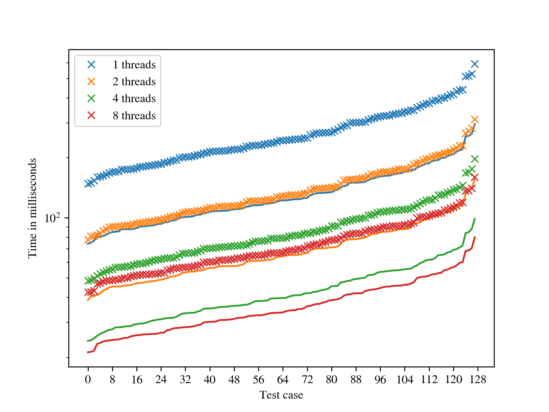
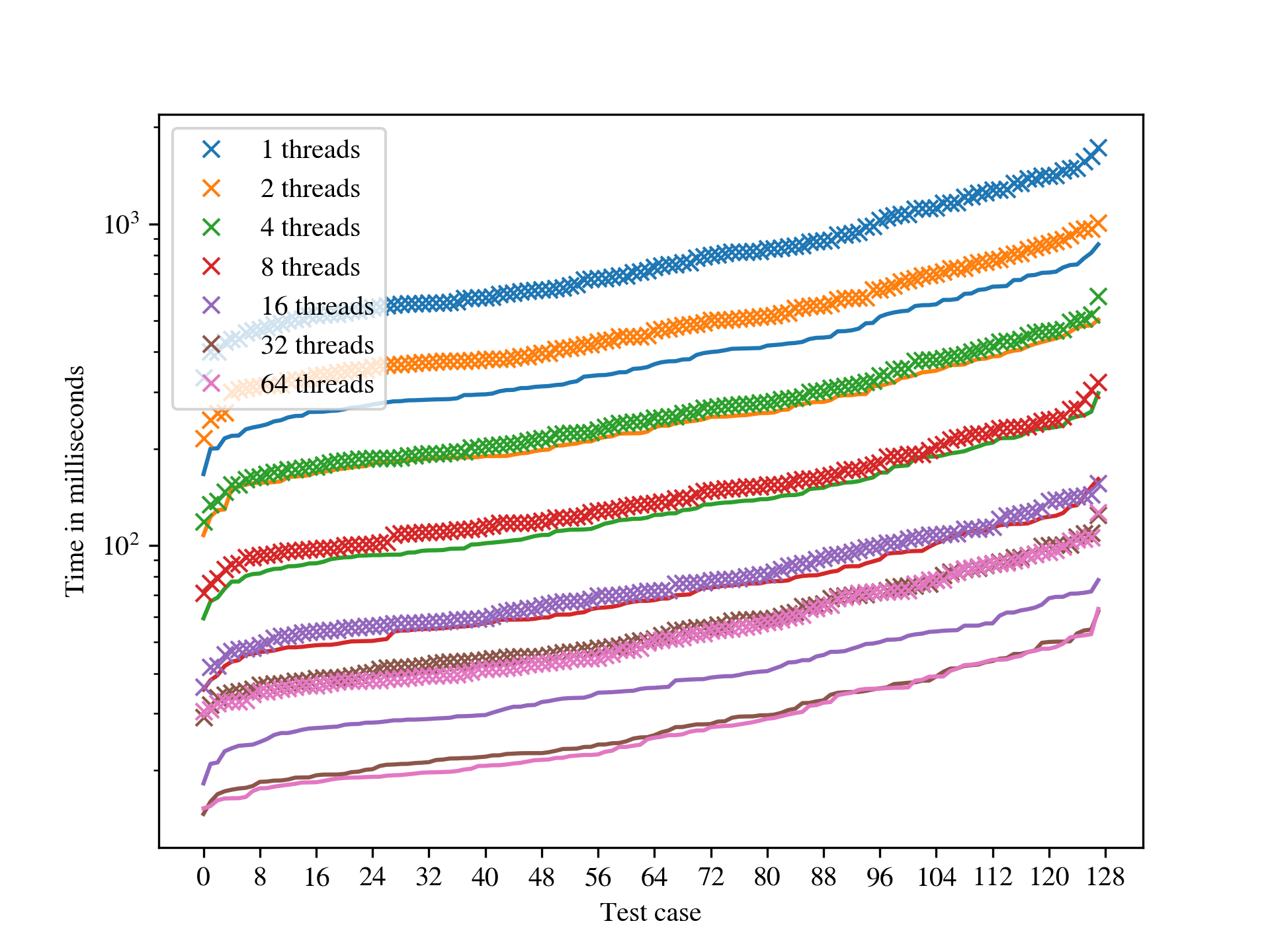
A.2 The impact of presentation length on the low-index congruences algorithm

In this section we present some experimental evidence about how the length of a presentation impacts the performance of the low-index congruences algorithm. If $\mathcal{P}=\langle A\mid R\rangle$ is a monoid presentation, then we refer to the sum $\sum_{(u,v)\in R}|u|+|v|$ of the lengths of the relation words in $R$ as the length of $\mathcal{P}$ . In Fig. A.2, a comparison of the length of a presentation for the full transformation monoid $T_{4}$ versus the runtime of the implementation of the low-index congruences algorithm in libsemigroups [53] is given. In Fig. 2(a), the initial input presentations were Iwahori’s presentation from [28, Theorem 9.3.1] for the full transformation monoid $T_{4}$ , and a complete rewriting system for $T_{4}$ output from the Froidure-Pin Algorithm [26]. Both initial presentations contain many redundant relations, these were removed $5$ at a time, and the time to compute the number of left congruences of $T_{4}$ with at most $16$ classes is plotted for each resulting presentation. We also attempted to perform the same computation with input Aizenstat’s presentation from [62, Ch. 3, Prop 1.7] (which has length $162$ ), but the computation was extremely slow.

In Fig. 2(b) and Fig. 2(c), a similar approach is taken. The initial input presentations in Fig. 2(b) and Fig. 2(c) were Fernandes’ presentations from [24, Theorems 2.6 and 2.7], respectively, and the outputs of the Froidure-Pin Algorithm [26] with the corresponding generating sets.

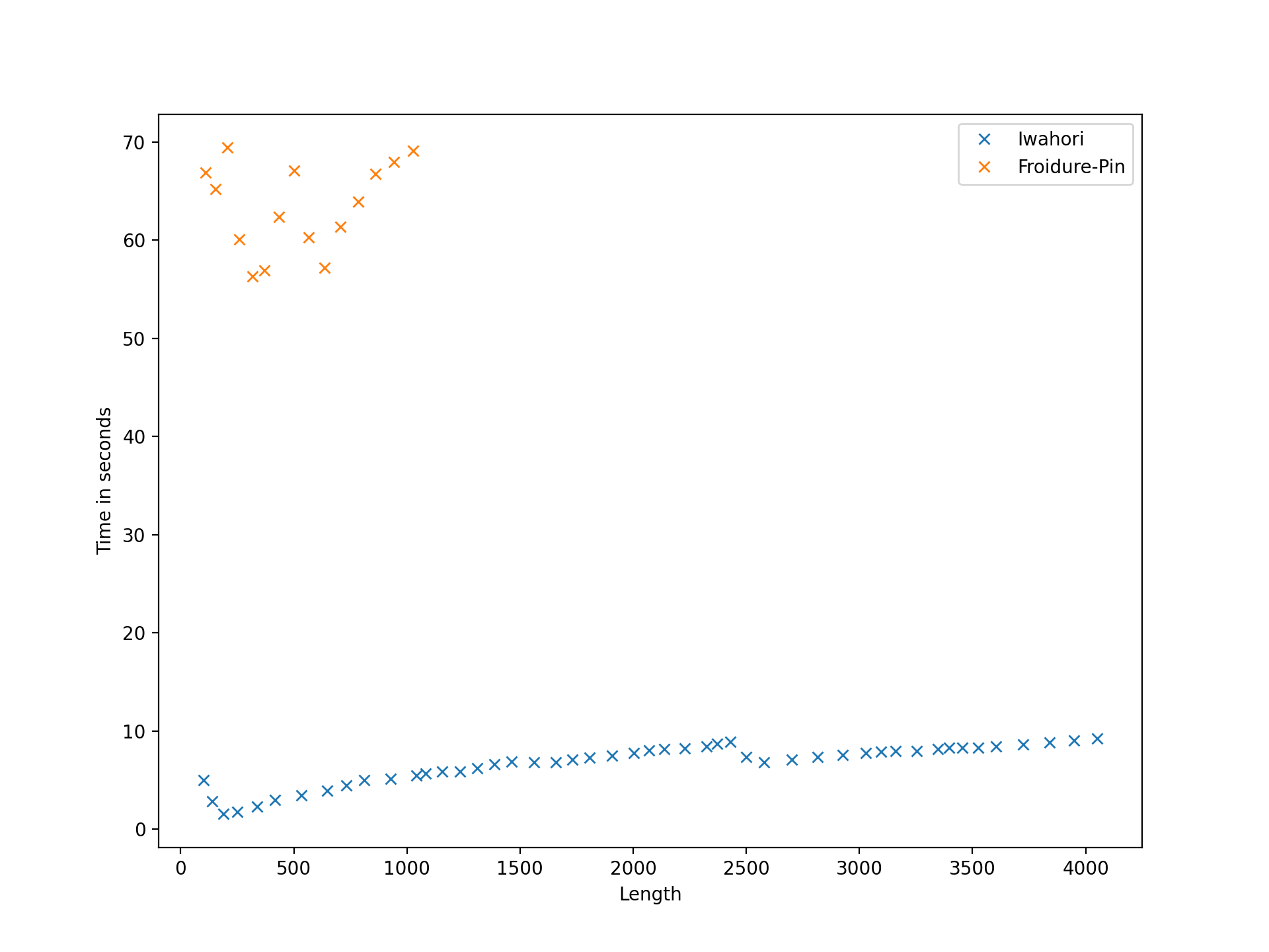
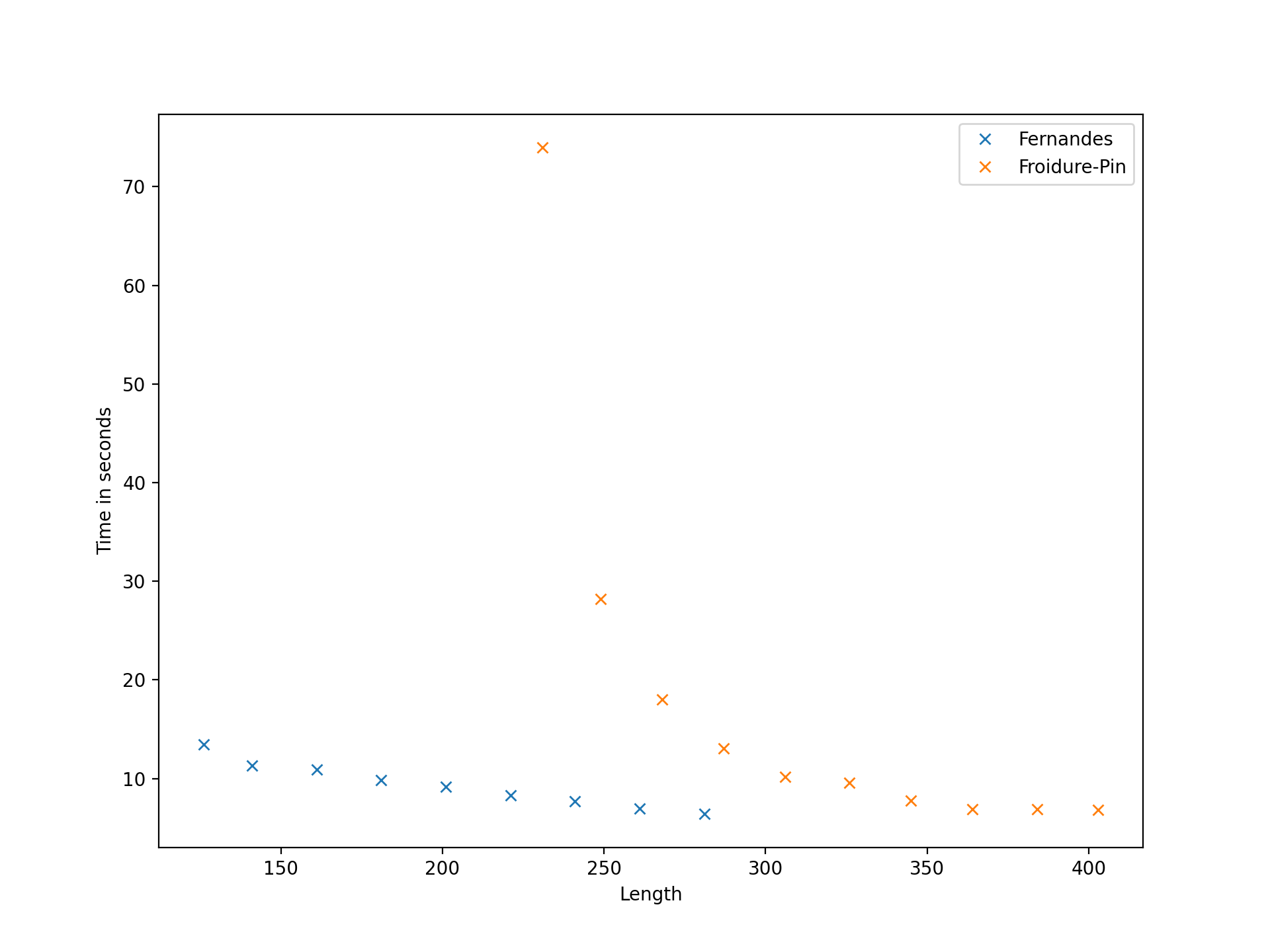
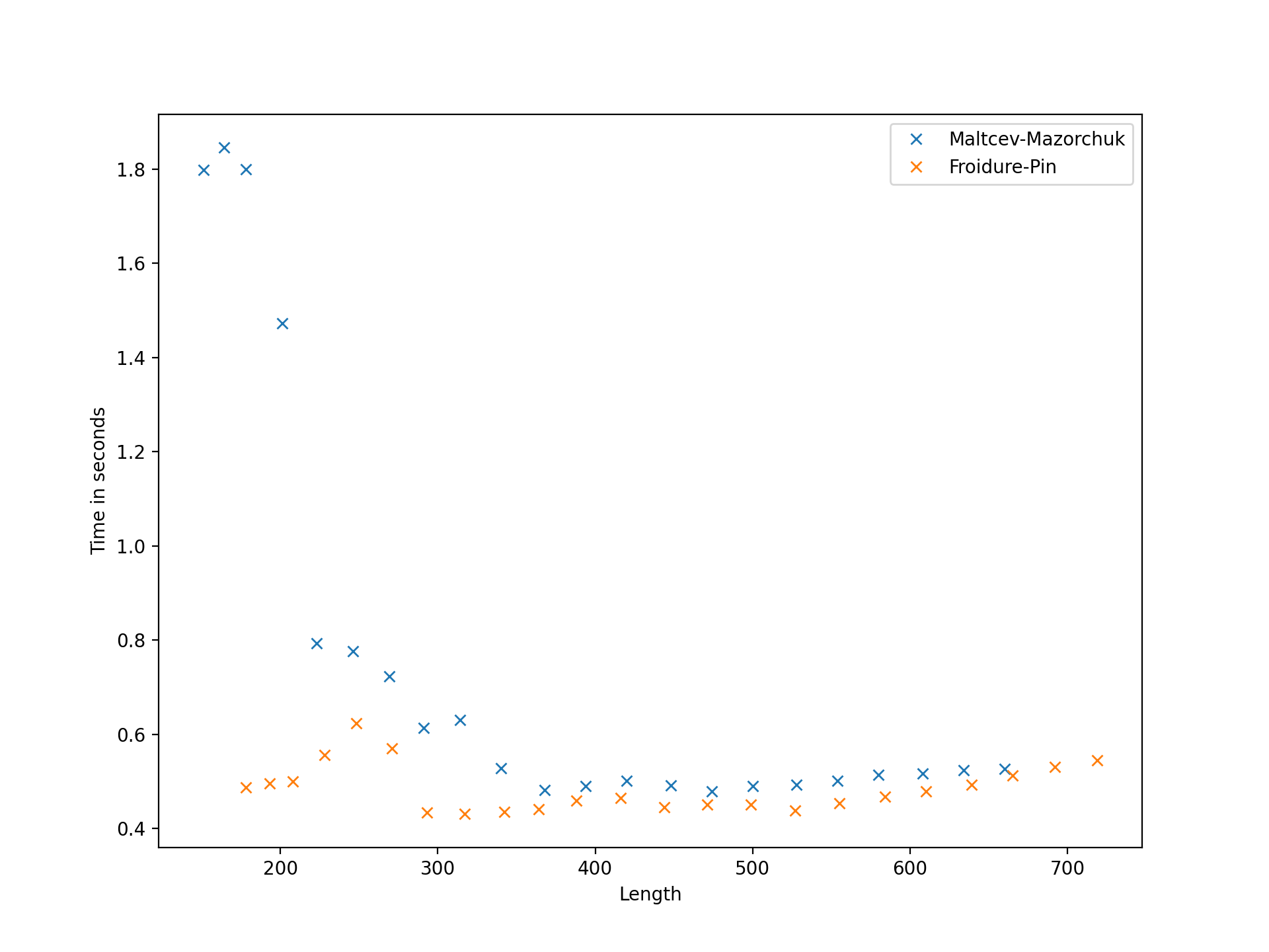
The outcome is mixed: in all of these examples the “human” presentations provide better performance than their “non-human” counterparts; for $T_{n}$ shorter means faster up to a point; for the first presentation for $\mathcal{CI}_{n}$ shorter means slower; for the second presentation for $\mathcal{CI}_{n}$ shorter means faster. There is only a single value for the computer generated presentation for $\mathcal{CI}_{n}$ with the second generating set because it was not straightforward to find redundant relations in this presentation. It might be worth noting that although the length of this presentation is ${\sim}16,000$ , the time taken is still considerably less than the fastest time using the first presentation.

A.3 1-sided congruences on finite monoids

In this section we present some data about the relative performance of the implementation of low-index congruences algorithm, Algorithm 7, and [25] in libsemigroups [53], Semigroups [54], and CREAM [58], respectively; see Tables B.1, A.1, A.2, A.3, and A.4.

Again, the outcome is somewhat mixed. Generally in the examples presented in this section, the low-index congruence algorithm as implemented in libsemigroups [53] is fastest for finding all right congruences, followed by CREAM [58] for the small examples, and Algorithm 7 from Semigroups [54] for larger values. For finding only principal congruences, again CREAM [58] is faster for smaller examples, and Semigroups [54] is faster for larger examples.

Given that CREAM [58] is tool for arbitrary finite algebras of type $(2^{m},1^{n})$ (i.e. with a finite number of binary and unary operations), it might be expected that specialised algorithms (such as those in this article) for semigroups and monoids would always perform better. There are two possible reasons for this. Firstly, as mentioned above, for some examples, the number of pairs output by Algorithm 7 is more or less the same as the maximum possible number; see Fig. A.3(a), Fig. A.4(a) and Fig. A.5(a). As such running Algorithm 7 prior to finding principal congruences, and then computing the joins, can increase the overall runtime. Secondly, the implementation in CREAM [58] is written almost entirely in C, and the main loop of the corresponding implementation in Semigroups [54] is written in the interpreted GAP [29] language. Specifically, the main loops in the implementation of Algorithm 7 in Semigroups [54], and the code for determining the set of principal congruences are written in GAP [29]. The code for forming all joins in Semigroups [54] is written in C++. Interpreted languages typically incur a performance penalty when compared to compiled languages.

$n$	low-index		Algorithm 7		Algorithm 7 + joins
$n$	mean	s.d.	mean	s.d.	mean	s.d.
1	$2.2\times 10^{-6}$	$1.8\times 10^{-6}$	$5.0\times 10^{-4}$	$2.0\times 10^{-4}$	$8.0\times 10^{-4}$	$4.0\times 10^{-4}$
2	$4.39\times 10^{-6}$	$0.14\times 10^{-6}$	$1.6\times 10^{-4}$	$0.3\times 10^{-4}$	$2.2\times 10^{-4}$	$1.1\times 10^{-4}$
3	$1.3\times 10^{-5}$	$0.2\times 10^{-5}$	$5.8\times 10^{-4}$	$0.7\times 10^{-4}$	$1.0\times 10^{-3}$	$0.4\times 10^{-3}$
4	$9.20\times 10^{-4}$	$0.10\times 10^{-4}$	$5.5\times 10^{-3}$	$0.8\times 10^{-3}$	$1.1\times 10^{-2}$	$0.2\times 10^{-2}$
5	$22.500\times 10^{0}$	$0.012\times 10^{0}$	$7.0\times 10^{-2}$	$0.6\times 10^{-2}$	Exceeded available memory
6	Exceeded available time		$1.23\times 10^{0}$	$0.11\times 10^{0}$	Exceeded available memory
7	Exceeded available time		$3.0\times 10^{1}$	$0.2\times 10^{1}$	Exceeded available memory

Table A.1: Runtimes in seconds for the low-index congruence algorithm (1 thread); Algorithm 7; and Algorithm 7 and all joins of principal right congruences of the Catalan monoids. For the low-index congruences algorithm, the values are the means of

100

trials using the presentation output by the Froidure-Pin Algorithm[26]. The values for Algorithm 7 (and all joins) are the means of

200

trials.

$n$	principal		all
$n$	mean	s.d.	mean	s.d.
1	$6\times 10^{-5}$	$4\times 10^{-5}$	$9.7\times 10^{-5}$	$3.0\times 10^{-4}$
2	$7\times 10^{-5}$	$3\times 10^{-5}$	$6.0\times 10^{-5}$	$4.0\times 10^{-5}$
3	$9\times 10^{-5}$	$6\times 10^{-5}$	$9.8\times 10^{-5}$	$6.0\times 10^{-5}$
4	$2.2\times 10^{-4}$	$1.1\times 10^{-4}$	$4.5\times 10^{-3}$	$1.0\times 10^{-3}$
5	$2.0\times 10^{-3}$	$0.7\times 10^{-3}$	Exceeded available memory
6	Seg. fault		Seg. fault
7	Seg. fault		Seg. fault

Table A.2: The means of runtimes (in seconds) for

200

trials of CreamPrincipalCongruences and CreamAllCongruences from CREAM [58] applied to the Catalan monoids (1 thread).

$n$	low-index		Algorithm 7		Algorithm 7 + joins
$n$	mean	s.d.	mean	s.d.	mean	s.d.
1	$2.2\times 10^{-6}$	$1.8\times 10^{-6}$	$5.0\times 10^{-4}$	$2.0\times 10^{-4}$	$8.0\times 10^{-4}$	$4.0\times 10^{-4}$
2	$5.6\times 10^{-6}$	$0.8\times 10^{-6}$	$1.0\times 10^{-3}$	$0.2\times 10^{-3}$	$1.0\times 10^{-3}$	$0.2\times 10^{-3}$
3	$4.9\times 10^{-5}$	$0.1\times 10^{-5}$	$4.31\times 10^{-3}$	$0.09\times 10^{-3}$	$4.6\times 10^{-3}$	$0.3\times 10^{-3}$
4	$3.555\times 10^{-2}$	$0.009\times 10^{-2}$	$3.9\times 10^{-2}$	$0.5\times 10^{-2}$	$5.1\times 10^{-2}$	$0.5\times 10^{-2}$
5	$3.364\times 10^{1}$	$0.004\times 10^{1}$	$5.33\times 10^{-1}$	$0.08\times 10^{-1}$	$2.763\times 10^{1}$	$0.012\times 10^{1}$
6	Exceeded available time		$9.39\times 10^{0}$	$0.19\times 10^{0}$	Exceeded available memory
7	Exceeded available time		$2.95\times 10^{2}$	-	Exceeded available memory

Table A.3: Runtimes in seconds for low-index congruences algorithm (1 thread); Algorithm 7; and Algorithm 7 and all joins of principal right congruences of the monoids

O_{n}

of order preserving transformations on

\{1,\ldots,n\}

. For the low-index congruences algorithm, the values are the means of

100

trials using the presentation from [5, Section 2] for

n\geq 3

and using the output of the Froidure-Pin Algorithm [26] for

n<3

. The values for Algorithm 7 (and all joins) are the means of

200

trials.

$n$	principal		all
$n$	mean	s.d.	mean	s.d.
1	$6\times 10^{-5}$	$4\times 10^{-5}$	$9.7\times 10^{-5}$	$3.0\times 10^{-4}$
2	$2.7\times 10^{-4}$	$0.6\times 10^{-4}$	$1.2\times 10^{-4}$	$0.1\times 10^{-4}$
3	$1.72\times 10^{-4}$	$0.06\times 10^{-4}$	$2.05\times 10^{-4}$	$0.05\times 10^{-4}$
4	$1.475\times 10^{-3}$	$0.015\times 10^{-3}$	$1.435\times 10^{-2}$	$0.007\times 10^{-2}$
5	$1.112\times 10^{-1}$	$0.011\times 10^{-1}$	$3.08\times 10^{1}$	$0.14\times 10^{1}$
6	$1.6\times 10^{1}$	$0.1\times 10^{1}$	Exceeded available memory
7	Seg. fault		Seg. fault

Table A.4: The means of runtimes (in seconds) for

200

trials of CreamAllPrincipalCongruences and CreamAllCongruences from CREAM [58] applied to the monoids

O_{n}

of order preserving transformations of

\{1,\ldots,n\}

(1 thread).

A.4 Low index subgroups

In this section, we compare the performance of: the implementation of the low-index congruences algorithm in libsemigroups [53]; the function LowIndexSubgroups in GAP [29]; the function permutation_reps from the C++ library 3Manifolds [15]; see Table A.5. The authors thank Derek Holt for suggesting the examples in this section. It is important to note that the implementation in libsemigroups [53] has no optimizations for groups, and that the inputs to libsemigroups [53] are monoid presentations; while the input to [15] and GAP [29] are group presentations. For details of the particular presentations used please see https://github.com/libsemigroups/libsemigroups/tree/main/benchmarks/sims.

group	index	subgroups	3manifolds [15]	GAP [29]	libsemigroups [53]
$(2,3,7)$ -triangle	$50$	$1,747$	$8.94\times 10^{-2}$	$4.20\times 10^{1}$	$1.76\times 10^{-1}$
4-generated braid group	$12$	$21$	$9.87\times 10^{-1}$	$1.11\times 10^{0}$	$2.02\times 10^{-1}$
modular group	$23$	$109,859$	$3.79\times 10^{-1}$	$1.26\times 10^{2}$	$4.39\times 10^{-1}$
fundamental group of K11n34	$7$	$52$	$7.01\times 10^{-1}$	$1.50\times 10^{0}$	$1.06\times 10^{0}$
Heineken	$8$	$3$	$2.26\times 10^{0}$	$9.5\times 10^{-1}$	$1.81\times 10^{0}$
fundamental group of K15n12345	$7$	$40$	$4.47\times 10^{-1}$	$2.12\times 10^{0}$	$6.33\times 10^{-1}$
fundamental group of o9 $\mbox{}_{15405}$	$9$	$38$	$2.10\times 10^{0}$	$1.65\times 10^{0}$	$1.68\times 10^{0}$

Table A.5: The time to determine subgroups up to some index for some groups. All times are in seconds. The indicated times are the mean values of between

10

and

100

trials. Standard deviations not included due to lack of space. Note that both 3manifolds [15] and libsemigroups [53] can be multithreaded with a corresponding decrease in the runtime. The fastest times are highlighted in green, the next fastest in orange, and the slowest in red.

A.5 2-sided congruences of finite monoids

In this section we present a comparison of the performance of computing the distinct 2-sided principal congruences of a selection of finite monoids. We compare several different versions of Semigroups [54] for GAP [29] that contain different optimisations. Semigroups [54] v3.4.1 contains none of the optimisations from the present paper, v4.0.2 uses Algorithm 7 where possible, and v5.3.0 uses Algorithm 7 and some further improvements to the code for finding distinct principal congruences. All computations in this section are single-threaded. We would have liked to include a comparison with CREAM [58] also, but unfortunately CREAM [58] suffers a segmentation fault (i.e. abnormal termination of the entire GAP [29] programme) on almost every input with more than approximately $400$ elements. This could have been circumvented, but due to time limitations, it was not. See Fig. A.3, Fig. A.4, Fig. A.5, and Table A.6.

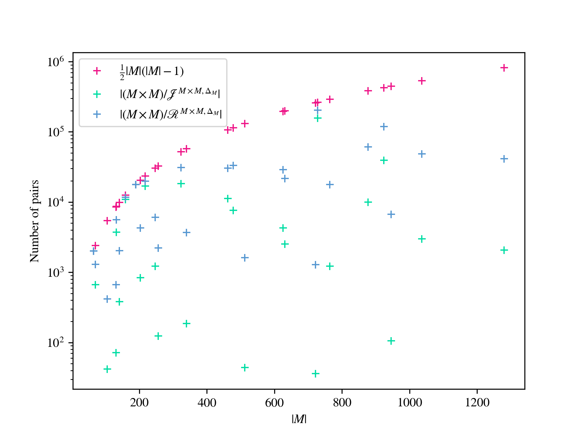
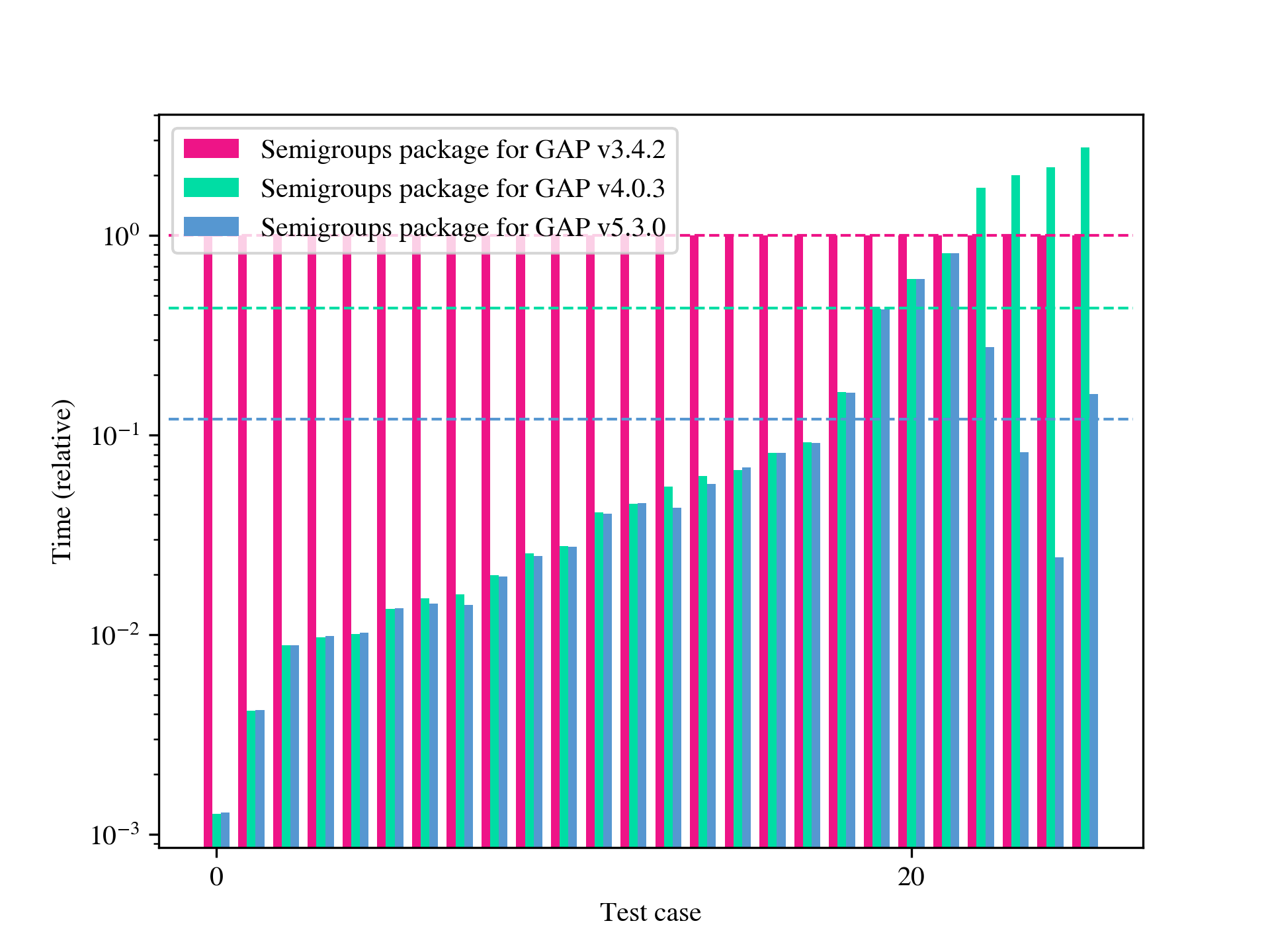
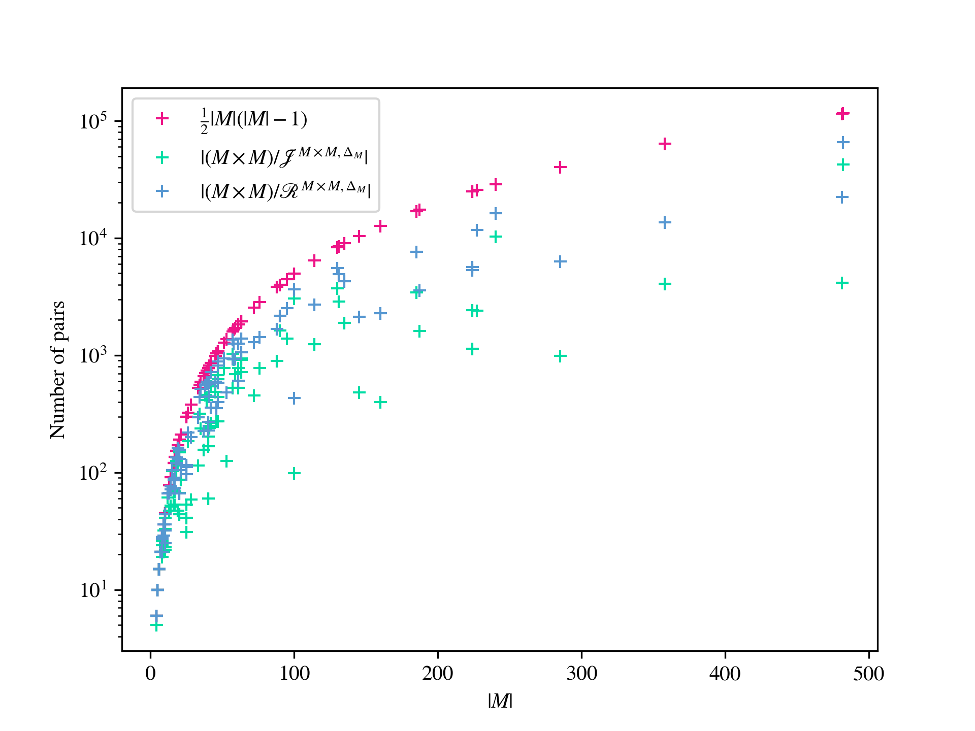
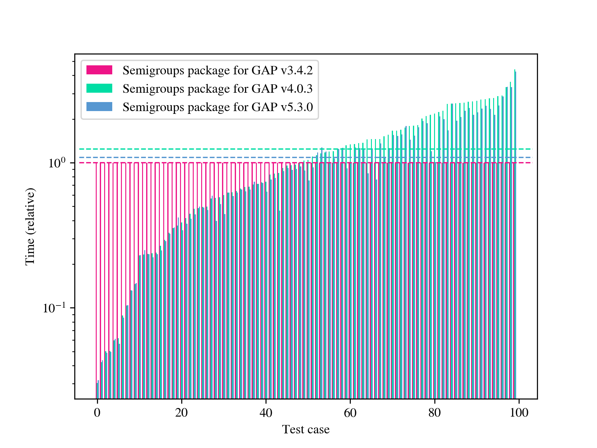
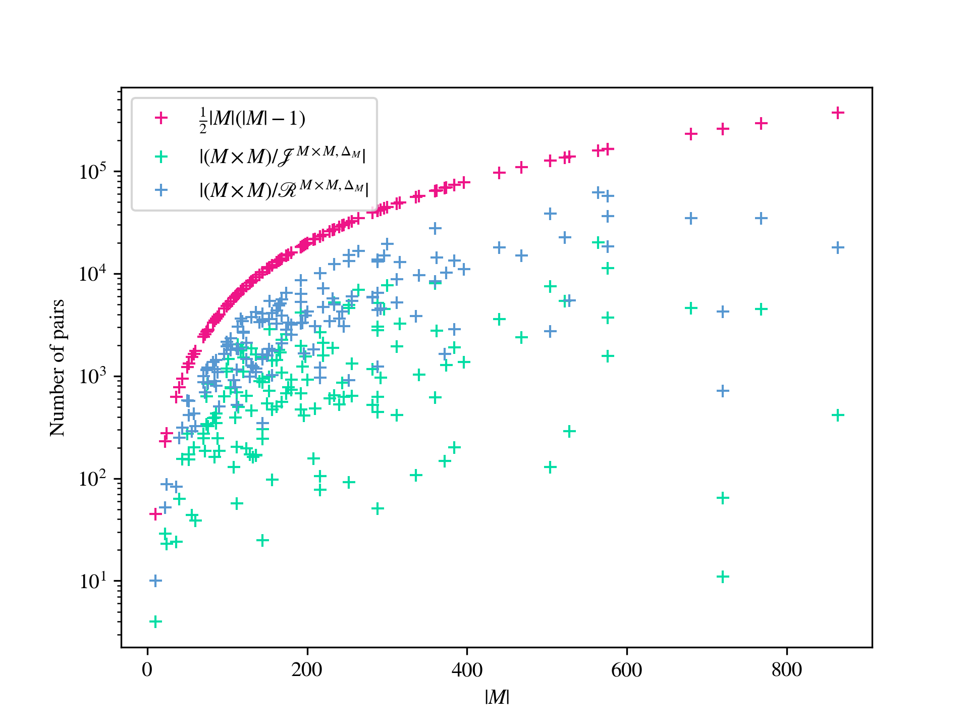
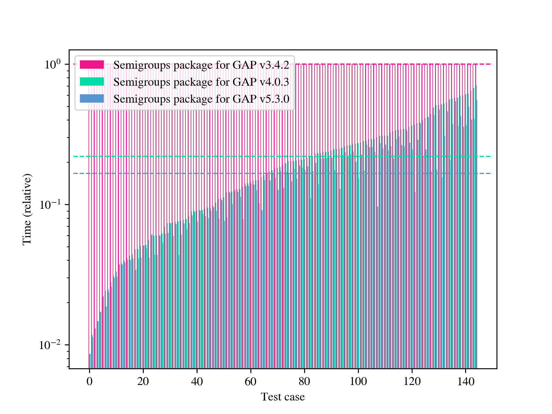
Monoid = $M_{n}$	$n$	$\|M_{n}\|$	$\|\mathcal{L}\|$	CREAM [58]		Semigroups [54]		libsemigroups [53]
Monoid = $M_{n}$	$n$	$\|M_{n}\|$	$\|\mathcal{L}\|$	mean	s.d.	mean	s.d.	mean	s.d.
Gossip	$3$	$11$	$84$	$6.0\times 10^{-4}$	$1.0\times 10^{-4}$	$5.2\times 10^{-3}$	$0.2\times 10^{-3}$	$1.87\times 10^{-4}$	$0.08\times 10^{-4}$
Jones	$4$	$14$	$9$	$5.0\times 10^{-4}$	$1.0\times 10^{-4}$	$1.2\times 10^{-2}$	$0.2\times 10^{-2}$	$3.5\times 10^{-5}$	$0.2\times 10^{-5}$
Brauer	$2$	$3$	$3$	$3.7\times 10^{-4}$	$0.6\times 10^{-4}$	$2.1\times 10^{-3}$	$0.4\times 10^{-3}$	$3.8\times 10^{-6}$	$0.4\times 10^{-6}$
Partition	$2$	$15$	$13$	$4.5\times 10^{-4}$	$0.8\times 10^{-4}$	$6.9\times 10^{-3}$	$0.9\times 10^{-3}$	$3.4\times 10^{-5}$	$0.5\times 10^{-5}$
Full PBR	$1$	$16$	$167$	$1.4\times 10^{-3}$	$0.2\times 10^{-3}$	$1.2\times 10^{-2}$	$0.2\times 10^{-2}$	$2.73\times 10^{-4}$	$0.07\times 10^{-4}$
Symmetric group	$4$	$24$	$4$	$1.4\times 10^{-3}$	$0.3\times 10^{-3}$	$4.0\times 10^{-3}$	$0.3\times 10^{-3}$	$5.5\times 10^{-5}$	$0.8\times 10^{-5}$
Full transformation	$3$	$27$	$7$	$1.6\times 10^{-3}$	$0.3\times 10^{-3}$	$5.3\times 10^{-3}$	$0.6\times 10^{-3}$	$8.6\times 10^{-5}$	$0.9\times 10^{-5}$
Symmetric inverse	$3$	$34$	$7$	$3.8\times 10^{-3}$	$0.4\times 10^{-3}$	$8.7\times 10^{-3}$	$0.9\times 10^{-\ 3}$	$9.6\times 10^{-5}$	$0.4\times 10^{-5}$
Jones	$5$	$42$	$6$	$7.5\times 10^{-3}$	$0.2\times 10^{-3}$	$9.0\times 10^{-2}$	$8.0\times 10^{-2}$	$3.8\times 10^{-4}$	$0.1\times 10^{-4}$
Motzkin	$3$	$51$	$10$	$1.5\times 10^{-2}$	$0.1\times 10^{-2}$	$1.4\times 10^{-1}$	$0.9\times 10^{-1}$	$8.2\times 10^{-3}$	$0.05\times 10^{-3}$
Partial transformation	$3$	$64$	$7$	$3.8\times 10^{-2}$	$0.1\times 10^{-2}$	$2.0\times 10^{-2}$	$1.0\times 10^{-2}$	$1.96\times 10^{-3}$	$0.02\times 10^{-3}$
Partial brauer	$3$	$76$	$16$	$6.8\times 10^{-2}$	$0.5\times 10^{-2}$	$5.4\times 10^{-2}$	$0.3\times 10^{-2}$	$5.06\times 10^{-3}$	$0.05\times 10^{-3}$
Brauer	$4$	$105$	$19$	$2.52\times 10^{-1}$	$0.06\times 10^{-1}$	$2.0\times 10^{-2}$	$0.1\times 10^{-2}$	$4.3\times 10^{-3}$	$0.1\times 10^{-3}$
Symmetric group	$5$	$120$	$3$	$4.60\times 10^{-1}$	$0.08\times 10^{-1}$	$2.9\times 10^{-2}$	$0.3\times 10^{-2}$	$1.27\times 10^{-2}$	$0.01\times 10^{-2}$
Jones	$6$	$132$	$10$	$7.14\times 10^{-1}$	$0.08\times 10^{-1}$	$1.001\times 10^{0}$	$0.007\times 10^{0}$	$6.22\times 10^{-3}$	$0.03\times 10^{-3}$
Partition	$3$	$203$	$16$	$4.08\times 10^{0}$	$0.02\times 10^{0}$	$2.7\times 10^{-1}$	$0.2\times 10^{-1}$	$2.82\times 10^{-2}$	$0.02\times 10^{-2}$
Symmetric inverse	$4$	$209$	$11$	$4.65\times 10^{0}$	$0.02\times 10^{0}$	$7.0\times 10^{-2}$	$0.5\times 10^{-2}$	$4.34\times 10^{-3}$	$0.04\times 10^{-3}$
Full transformation	$4$	$256$	$11$	$9.65\times 10^{0}$	$0.05\times 10^{0}$	$7.7\times 10^{-2}$	$0.4\times 10^{-2}$	$1.007\times 10^{-1}$	$0.006\times 10^{-1}$
Motzkin	$4$	$323$	$11$	$2.54\times 10^{1}$	$0.01\times 10^{1}$	$8.9\times 10^{0}$	$0.1\times 10^{0}$	$3.38\times 10^{1}$	$0.03\times 10^{1}$
Jones	$7$	$429$	$7$	$8.56\times 10^{1}$	$0.02\times 10^{1}$	$1.72\times 10^{1}$	$0.02\times 10^{1}$	$1.54\times 10^{-1}$	$0.02\times 10^{-1}$

Table A.6: Performance comparison of CREAM [58], the algorithm described in Section 7 as implemented in the Semigroups [54] package for GAP [29], and the algorithm described in Section 5.2 as implemented in libsemigroups [53] for computing all 2-sided congruences (1 thread). All times are in seconds, and the fastest times are highlighted in green, the next fastest in orange, and the slowest in red.

Appendix B Congruence statistics

In this appendix we provide the numbers of finite index congruences of some well-known finite and infinite finitely presented monoids in a number of tables. By searching for these numbers in the [57] and in the literature, it appears that many of them were not previously known.

$n$	$\|C_{n}\|$	principal	minimal	all
1	1	0	0	1
2	2	1	0	2
3	5	8	3	11
4	14	67	6	575
5	42	641	10	5,295,135
6	132	6,790	15	?
7	429	76,568	21	?
⋮	⋮	⋮	⋮	⋮
$n$	$(2n)!/(n!(n+1)!)$	?	$(n+1)(n+2)/2$ ?	?
	A000108	OEIS	OEIS	OEIS

Table B.1: The numbers of principal, minimal, and all right congruences of the Catalan monoids

C_{n}

[31] for some small values of

n

		left congruences
$n$	$\|O_{n}\|$	principal	minimal	all
1	1	0	0	1
2	3	2	1	3
3	10	18	3	31
4	35	138	6	2,634
5	126	1,055	10	6,964,196
6	462	8,234	15	?
7	1,716	?	?	?
⋮	⋮	⋮	⋮	⋮
$n$	$\binom{2n+1}{n+1}$	?	$n(n+1)/2$ ?	?
	A001700	OEIS	A253145	OEIS

right congruences
principal	minimal	all
0	0	1
3	3	5
18	6	25
116	10	385
853	15	37,951
6,707	21
54,494	28	?
⋮	⋮	⋮
?	$n(n+1)/2$ ?	?
OEIS	A253145	OEIS

Table B.2: The numbers of principal, minimal, and all left and right congruences of the monoids

O_{n}

of order-preserving transformations of an

n

-chain for some small values of

n

		left congruences
$n$	$\|OR_{n}\|$	principal	minimal	all
1	1	0	0	1
2	4	3	1	4
3	17	27	3	94
4	66	222	6	32,571
5	247	1,831	10	?
6	918	15,137	15	?
⋮	⋮	⋮	⋮	⋮
$n$	$\binom{2n}{n}$	?	$n(n+1)/2$ ?	-
	A045992	OEIS	OEIS	OEIS

right congruences
principal	minimal	all
0	0	1
4	4	7
25	9	54
176	16	1,335
1,382	25	?
11,575	36	?
⋮	⋮	⋮
?	$n^{2}$ ?	?
OEIS		OEIS

Table B.3: The numbers of principal, minimal, and all left and right congruences of the monoids

OR_{n}

of order-preserving or -reversing transformations of an

n

-chain for some small values of

n

		left congruences
$n$	$\|PO_{n}\|$	principal	minimal	all
1	2	1	0	2
2	8	8	3	9
3	38	67	6	142
4	192	653	10	16,239
5	1,002	7,314	15	?
⋮	⋮	⋮	⋮	⋮
$n$	$2\sum_{k=0}^{n-1}\binom{n-1}{k}\binom{n+k}{k}$	?	?	?
	A002003	OEIS	OEIS	OEIS

right congruences
principal	minimal	all
1	0	2
12	6	18
172	28	10,036
2,612	120	?
40,074	496	?
⋮	⋮	⋮
?	?	?
OEIS	OEIS	OEIS

Table B.4: The numbers of principal, minimal, and all left and right congruences of the monoids

PO_{n}

of partial order-preserving transformations of an

n

-chain for some small values of

n

		left congruences
$n$	$\|POR_{n}\|$	principal	minimal	all
1	2	1	0	2
2	9	9	3	11
3	54	79	6	306
4	323	874	10	104,400
5	1,848	?	?	?
⋮	⋮	⋮	⋮	⋮
$n$	$2\|PO_{n}\|-(1+\sum_{k=1}^{n}\binom{n}{k}n)$	?	?	?
	OEIS	OEIS	OEIS	OEIS

right congruences
principal	minimal	all
1	0	2
13	6	23
191	28	35,598
3,195	120	?
54,785	496	?
⋮	⋮	⋮
?	?	?
OEIS	OEIS	OEIS

Table B.5: The numbers of principal, minimal, and all left and right congruences of the monoids

POR_{n}

of partial order-preserving or -reversing transformations of an

n

-chain for some small values of

n

$n$	$\|POI_{n}\|$	principal	minimal	all
1	2	1	0	2
2	6	7	3	8
3	20	46	6	99
4	70	330	10	8,146
5	252	2,602	15	18,732,669
6	924	21,900	21	?
⋮	⋮	⋮	⋮	⋮
$n$	$\binom{2n}{n}$	?	$(n+1)(n+2)/2$	-
	A000984	OEIS	A253145	OEIS

$n$	$\|PODI_{n}\|$	principal	minimal	all
1	2	1	0	2
2	7	8	3	10
3	30	56	6	232
4	123	453	10	64,520
5	478	4,032	15	?
6	1,811	37,410	21	?
⋮	⋮	⋮	⋮	⋮
$n$		?	$(n+1)(n+2)/2$	?
	OEIS	OEIS	OEIS	OEIS

Table B.6: The numbers of principal, minimal, and all left/right congruences of the monoids

POI_{n}

and

PODI_{n}

of order-preserving, and order-preserving and -reversing, respectively, partial permutations of an

n

-chain for some small values of

n

$n$	$\|POPI_{n}\|$	principal	minimal	all
1	2	1	0	2
2	7	8	3	10
3	31	56	6	220
4	141	460	10	57,357
5	631	4,322	15	?
⋮	⋮	⋮	⋮	⋮
$n$		?	$(n+1)(n+2)/2$ ?	?
	A289719	OEIS	OEIS	OEIS

$n$	$\|PORI_{n}\|$	principal	minimal	all
1	2	1	0	2
2	7	8	3	10
3	34	59	6	274
4	193	506	10	188,740
5	1,036	5,347	15	?
⋮	⋮	⋮	⋮	⋮
$n$		?	$(n+1)(n+2)/2$ ?	?
	A289720	OEIS	OEIS	?

Table B.7: The numbers of principal, minimal, and all left/right congruences of the monoids

POPI_{n}

and

PORI_{n}

of orientation-preserving, and orientation-preserving or -reversing, respectively, partial permutations of an

n

-chain for some small values of

n

		left congruences
$n$	$\|PT_{n}\|$	principal	minimal	all
1	2	1	1	2
2	9	9	3	11
3	64	84	6	371
4	625	1,086	10	335,497
⋮	⋮	⋮	⋮	⋮
$n$	$(n+1)^{n}$	?	$n(n+1)/2$ ?	?
	A289720	OEIS	OEIS	?

right congruences
principal	minimal	all
1	1	2
13	6	23
237	28	92,703
6,398	120	?
⋮	⋮	⋮
?	?	?
OEIS	OEIS	OEIS

Table B.8: The numbers of principal, minimal, and all left and right congruences of the monoids

PT_{n}

of all partial transformations on an

n

-set.

		left congruences
$n$	$\|T_{n}\|$	principal	minimal	all
1	1	0	0	1
2	4	3	1	4
3	27	32	3	120
4	256	370	6	120,121
5	3,125	5,892	10	?
⋮	⋮	⋮	⋮	⋮
$n$	$n^{n}$	?	$n(n+1)/2$ ?	?
	A000312	OEIS	OEIS	OEIS

right congruences
principal	minimal	all
0	0	1
4	4	7
44	16	287
900	64	22,069,828
28,647	256	?
⋮	⋮	⋮
?	$2^{2n-2}$	?
OEIS	OEIS	OEIS

Table B.9: The numbers of principal, minimal, and all left and right congruences of the monoids

T_{n}

of all transformations on an

n

-set.

$n$	$\|I_{n}\|$	principal	minimal	all
1	2	1	1	2
2	7	8	3	10
3	34	59	6	274
4	209	516	10	195,709
5	1,546	5,667	15	?
⋮	⋮	⋮	⋮	⋮
$n$	$\sum_{k=0}^{n}\binom{n}{k}^{2}k!$	?	$n(n+1)/2$ ?	?
	A002720	OEIS	OEIS	OEIS

Table B.10: The numbers of principal, minimal, and all left and right congruences of the symmetric inverse monoids

I_{n}

of all partial permutations on an

n

-set.

$n$	$\|J_{n}\|$	principal	minimal	all
1	1	0	0	1
2	2	1	1	2
3	5	6	3	9
4	14	30	7	79
5	42	118	15	2,157
6	132	602	29	4,326,459
7	429	2,858	105	?
⋮	⋮	⋮	⋮	⋮
$n$	$(2n)!/(n!(n+1)!)$	?	?	?
	A002720	OEIS	OEIS	OEIS

$n$	$\|B_{n}\|$	principal	minimal	all
1	1	0	0	1
2	3	2	1	3
3	15	16	6	48
4	105	142	18	103,406
5	945	1,636	120	?
⋮	⋮	⋮	⋮	⋮
$n$	$(2n-1)!!$	?	?	?
	A001147	OEIS	OEIS	OEIS

Table B.11: The numbers of principal, minimal, and all left and right congruences of the Jones (or Temperley-Lieb) monoids

J_{n}

and the Brauer monoids

B_{n}

of degree

n

$n$	$\|M_{n}\|$	principal	minimal	all
1	2	1	1	2
2	9	18	6	37
3	51	188	18	15,367
4	323	2,332	66	?
⋮	⋮	⋮	⋮	⋮
$n$	$(2n)!/(n!(n+1)!)\sum_{k=0}^{n}\binom{2n}{2k}$	?	?	?
	A026945	OEIS	OEIS	OEIS

$n$	$\|I_{n}^{*}\|$	principal	minimal	all
1	1	0	0	1
2	3	2	1	3
3	25	26	9	108
4	339	627	49	?
⋮	⋮	⋮	⋮	⋮
$n$	?	?	$(2^{n}-1)^{2}$ ?	?
	A026945	OEIS	OEIS	?

Table B.12: The numbers of principal, minimal, and all left and right congruences of the Motzkin monoids

M_{n}

and the dual symmetric inverse monoids

I_{n}^{*}

of degree

n

	2	3	4	5	6	7	8	9	10	11	12
1	1	1	1	1	1	1	1	1	1	1	1
2	7	15	31	63	127	255	511	1023	2047	4095	8191
3	27	102	351	1146	3627	11262	34511	105186	318627	962022	2898351
4	94	616	3346	16360	75034	330256	1414066	5940760	24627274	101123296	412378786
5	275	3126	26483	189420	1220045	7335126	42061343	233221440	1261948865	6705793626	35151482003
6	833	16914	222425	2289148	20263055	162391586	1214730797	8646767880	59332761467	396002654398
7	2307	91072	1927625	28829987	349842816	3703956326	35686022019	321211486801
8	6488	491767	36892600	995133667	17898782992	257691084789	3222193441904
9	18207	2583262	955309568	457189474269
10	52960	14222001	12834025602
11	156100	87797807
12	462271	676179934
13	1387117	7373636081
14	4330708	120976491573
15	14361633
16	51895901
17	209067418
18	955165194
19	4777286691
20	24434867465
21	114830826032
22	499062448513

Table B.13: Numbers of 2-sided congruences of the free monoids; see also [6, Appendix C] for the corresponding results in the free semigroup. The columns correspond to the number of generators and the rows to the index of the congruences, so that the value in row

i

and column

j

is the number of 2-sided congruences with index at most

i

of the free monoid with

j

-generators.

$n$	index $\leq 2$	index $\leq 3$	index $\leq 4$	index $\leq 5$	index $\leq 6$	index $\leq 7$	index $\leq 8$
3	29	484	6,896	103,204	1,773,360	35,874,182	849,953,461
4	67	2,794	106,264	4,795,980	278,253,841	20,855,970,290	-
5	145	14,851	1,496,113	198,996,912	37,585,675,984	-	-
6	303	77,409	20,526,128	7,778,840,717	-	-	-
7	621	408,024	281,600,130	-	-	-	-
8	1,259	2,201,564	-	-	-	-	-
$a_{n}$	$2a_{n-1}+2n+3$	?	?	?	?	?	?

Table B.14: The number of left and right congruences of the Plactic monoid with

n

-generators for some small values of

n