22email: dachen.cn@hotmail.com 33institutetext: Jean-Marie Mirebeau 44institutetext: Department of Mathematics, Centre Borelli, ENS Paris-Saclay, CNRS, University Paris-Saclay, 91190, Gif-sur-Yvette, France.
44email: jean-marie.mirebeau@math.u-psud.fr
55institutetext: Minglei Shu 66institutetext: Shandong Artificial Intelligence Institute, Qilu University of Technology (Shandong Academy of Sciences), 250014 Jinan, China.
66email: shuml@sdas.org
77institutetext: Laurent D. Cohen 88institutetext: University Paris Dauphine, PSL Research University, CNRS, UMR 7534, CEREMADE, 75016 Paris, France
88email: cohen@ceremade.dauphine.fr
Computing Geodesic Paths Encoding a Curvature Prior for Curvilinear Structure Tracking
Abstract
In this paper, we introduce an efficient method for computing curves minimizing a variant of the Euler-Mumford elastica energy, with fixed endpoints and tangents at these endpoints, where the bending energy is enhanced with a user defined and data-driven scalar-valued term referred to as the curvature prior. In order to guarantee that the globally optimal curve is extracted, the proposed method involves the numerical computation of the viscosity solution to a specific static Hamilton-Jacobi-Bellman (HJB) partial differential equation (PDE). For that purpose, we derive the explicit Hamiltonian associated to this variant model equipped with a curvature prior, discretize the resulting HJB PDE using an adaptive finite difference scheme, and solve it in a single pass using a generalized Fast-Marching method. In addition, we also present a practical method for estimating the curvature prior values from image data, designed for the task of accurately tracking curvilinear structure centerlines. Numerical experiments on synthetic and real image data illustrate the advantages of the considered variant of the elastica model with a prior curvature enhancement in complex scenarios where challenging geometric structures appear.
Keywords:
Variant of the Euler-Mumford Elastica Model Curvature Prior Second-order Geodesic Path Fast-Marching Method Curvilinear Structure Tracking1 Introduction
Computing globally optimal geodesic curves, in domains equipped with complex metric cost functions, is a task efficiently achieved by solving the so-called eikonal equation, which is at the foundation of a line of works in the modeling of curvilinear shapes (Sethian, 1999; Peyré et al, 2010). Second-order geodesic models featuring curvature regularization allow imposing particular geometric priors (e.g. rigidity and smoothness) to the minimal geodesic paths, whose computation hence has become a core step to numerous practical applications. Typical examples include image analysis (Chen et al, 2017; Bekkers et al, 2015a), computer vision problems involving visual curve completion (Ben-Shahar and Ben-Yosef, 2014; Parent and Zucker, 1989) and perceptual grouping (Bekkers et al, 2018; Wertheimer, 1938), the study of optical illusions (Franceschiello et al, 2019), and robot motion planing (Mirebeau and Portegies, 2019; Kimmel and Sethian, 2001). This work is motivated by the fact that curvilinear structures exhibit significant geometric features such as orientation and curvature, which can be leveraged as crucial cues for computing geodesic paths to efficiently delineate these elongated shapes.
Approaches to computing globally optimal paths connecting two disjoint sets can be backtracked to Dijkstra’s shortest path algorithm (Dijkstra, 1959) in a finite graph. However, such a discrete setting may lead to metrication errors, especially for applications in image analysis. In order to address this issue, Cohen and Kimmel introduced a minimal geodesic model (Cohen and Kimmel, 1997) founded in a continuous PDE domain, and established the connection between the minimization of an energy defined as a weighted curve length (Caselles et al, 1997) and the viscosity solution to a static first-order HJB PDE. As a consequence, the computation of minimal geodesic paths is transferred to numerically solving the HJB PDE, which is efficiently addressed via Sethian’s pioneering work (Sethian, 1996, 1999) the Fast-Marching method.
The original geodesic model (Cohen and Kimmel, 1997) measures the length of regular curves in an isotropic manner, using weights depending on the local curve position but not on its orientation, which limits its practical applications. The introduction of anisotropic geometric models, and measures of path length depending on the orientation in a user-defined manner, is an important extension to the original geodesic model, which has deeply extended its applicable scope, leading to successful applications in image analysis and computer vision (Melonakos et al, 2008). For instance, curvilinear structure tracking can take advantage of anisotropic Riemannian models, by enhancing the geodesic metric with anisotropy features extracted from the elongated structures present in the processed image (Parker et al, 2002; Benmansour and Cohen, 2011; Jbabdi et al, 2008). Chen et al (2016) proposed to address the region-based active contour problem (Mumford and Shah, 1989) by computing the minimal geodesic path associated to a Randers metric (Randers, 1941) featuring a data-driven drift term. For geodesic models involving anisotropic metrics, the classical Fast-Marching method (Sethian, 1996) is no longer suitable for estimating the solutions to the respective HJB PDEs (Sethian and Vladimirsky, 2001, 2003). In order to bridge this gap, Mirebeau introduced variants of the Fast-Marching method which rely on adaptive stencil systems depending on the associated metrics, based on either the geometric tool of Lattice basis reduction (Mirebeau, 2014b, a) or the Voronoi’s first reduction technique (Mirebeau, 2019, 2018). In practice, those state-of-the-art generalized anisotropic Fast-Marching methods can address various anisotropic geodesic models, while achieving sufficient accuracy and requiring a low computational cost.


Second-order geodesic models, which use the path curvature as a regularizer of the weighted curve length, can be regarded as limit cases of anisotropic models defined over the configuration space of positions and orientations, see (Chen et al, 2017; Duits et al, 2018; Bekkers et al, 2015a; Mirebeau, 2018) for significant examples. Following the optimal control framework, the Euler-Mumford elastica, Reeds–Shepp car and Dubins car problems are respectively connected to the associated HJB PDEs, yielding efficient Fast-Marching schemes for finding curvature-penalized optimal curves (Mirebeau, 2018). An extension of these models allows computing curves which are boundaries of convex shapes, by controlling the sign of the curvature and the winding number of the path (Chen et al, 2021). In these works, the curvature penalization is regarded as a regularization term, whose importance is delicately balanced with an image data term, following the general principles of data fitting.
In practice, unfortunately, striking a good balance between the curvature regularization and the image data terms remains a challenging problem for these second-order geodesic models (Chen et al, 2017; Duits et al, 2018; Mirebeau, 2018), particularly in the presence of crossing structures, strongly bent segments, and complex image background content. In general, assigning high importance weights to curvature regularization usually corresponds to optimal paths favoring low curvature. On the other hand, such a setting may in turn introduce a bias to the underlying strongly curved segments, thus giving rise to unexpected results. Fig. 1 illustrates an example in an aerial image, where the goal is to extract a road joining two given points (red and blue dots), see Fig. 1a. In Fig. 1b, one can see that the geodesic path derived from the classical Euler-Mumford elastica model (Chen et al, 2017; Mirebeau, 2018) suffers from a shortcut problem, due to the unbalanced importance of the weights associated to the curvature regularization and to the image data. This shortcoming of the classical elastica model prevents its practical applications in complex scenarios. An alternative approach, explored in this paper and motivated by the drawback as mentioned above, is to compute geodesic paths whose curvature approximates some data-driven prior reference values and more generally to introduce data information in the new curvature term. An additional contribution is a collection of techniques to estimate these prior curvature values from the image data, and to extend and preprocess them for their use as an enhancement to the geodesic model. Fig. 1c illustrates an optimal path from the variant of the elastica model, equipped with a suitable curvature prior which enables the accurate extraction of the target road.
In (Mirebeau and Portegies, 2019), the authors illustrated how geodesic paths with a type of curvature prior could be computed using a modification of the Hamiltonian Fast-Marching (HFM) method (Mirebeau, 2018, 2019). However, the mathematical PDE framework, the construction of the numerical scheme, and the application scope of the geodesic models with embedded curvature prior were not investigated. In this paper, we describe the Hamiltonian of a variant of the Euler-Mumford elastica model featuring a curvature prior enhancement, and we illustrate related objects known as control sets. The Hamiltonian of this variant of the classical elastica model, referred to as the curvature prior elastica model, is then discretized, leading to a numerical method for solving the corresponding static first-order HJB PDE, and thus computing the globally optimal geodesic paths. Finally, we introduce a practical method for estimating the curvature prior values, designed to improve the performance of tracking curvilinear structures from challenging image data.
The remainder of this manuscript is organized as follows. We first review the classical Euler-Mumford elastica model, including the expression of the associated HJB PDE which is posed over the configuration space of positions and orientations, and the computation of the relevant minimal geodesic paths. Then we present the core of this work: the derivation of the Hamiltonian of a variant of the elastica model equipped with a curvature prior, the relevant static HJB PDE, and its implementation in the application of curvilinear structure tracking. Eventually, we present experimental results conducted on both synthetic and real images.
2 The Euler-Mumford Elastica Model
2.1 Background
The celebrated Euler-Mumford elastica model (Mumford, 1994; Nitzberg, 1990) characterizes smooth curves which minimize a functional featuring a length term and a bending energy term, in other words a curvature penalization. Let be the curvature of a smooth curve with non-vanishing velocity, where is a bounded domain. Given a data-driven cost function , the energy functional considered in the classical Euler-Mumford elastica model reads
| (1) |
where is the first-order derivative of the curve , and denotes the standard Euclidean norm over the space . The constant parameter controls the relative importance of the bending energy term , which penalizes curvature, w.r.t. the penalization of path length. By construction, Eq. 1 is invariant under smooth increasing re-parametrizations of the curve , and the second argument of is the unit tangent vector to the path. In the special case where is constant, the curves for which Eq. 1 is extremal correspond to the rest positions of elastic rods of suitable length (with their endpoints clamped), however this physical interpretation is lost for non-constant .


2.2 Reformulation via Orientation Lifting
A widely used strategy for addressing the classical Euler-Mumford elastica optimal curve problem is to lift a planar smooth curve into the higher dimensional configuration space of positions and orientations, see (Chen et al, 2017; Duits et al, 2018; Chambolle and Pock, 2019), where denotes the angular domain. In other words with periodic boundary conditions, and we can parametrize the unit circle via the unit vector for any angle . Furthermore, we denote by the tangent vector space to , and by the dual vector space of . Recall that is a smooth curve with non-vanishing velocity. Following the literature (Chen et al, 2017; Mirebeau, 2018; Duits et al, 2018), an orientation-lifted curve , whose physical projection is the given planar curve , can be constructed by introducing an angular function such that
| (2) |
This leads to an alternative representation of the curvature
| (3) |
Inserting this expression of the curvature into the energy defined in Eq. 1 yields an equivalent formula, measured along an orientation-lifted curve whose components and obey Eq. 2:
| (4) |
where is a positive cost function defined by
For the task of curvilinear structure tracking, as considered in this work, the value of should be relatively low in case the physical position is inside a curvilinear structure and the direction matches its local geometry at the position , i.e. is approximately tangent to its centerline at . Fig. 2 shows an example for the cost function derived from an image that consists of curvilinear structures. The construction and the numerical computation of is presented in Eq. 25 below, and relies on a tool known as the orientation score.
2.3 Elastica Metric and Control Sets
The energy formulated in Eq. 4 can be expressed in terms of a degenerate geodesic metric (Chen et al, 2017; Mirebeau, 2018), denoted by and referred to as the elastica metric. For any point and any non-zero vector this elastica metric is defined as
| (5) |
Note that this metric is not symmetric, since in general in view of the non-linear constraint , and thus the corresponding distance defined below (see Eq. 11) is likewise non-symmetric. Such asymmetric objects are often referred to as quasi-metrics and quasi-distances, but the prefix “quasi-” is dropped in this paper for the sake of readability.
Several mathematical objects can be attached to such a metric. The control sets , for all points , allow visualizing the geometry, see Fig. 3, and are defined as
| (6) |
The Hamiltonian is involved in the numerical computation of optimal geodesic paths through the HJB PDE, as formulated in next subsection, and is defined for any co-vector as
| (7) |
In the special case of the elastica metric, one can use Eq. 5 to obtain the explicit expressions of the control sets and Hamiltonian, see (Mirebeau, 2018) for the details of this computation. Specifically, for any point one has
| (8) |
For any co-vector one obtains
| (9) |
The following equivalent expression of the Hamiltonian, in integral form, is established in Mirebeau (2018)
| (10) |
where is the positive part of the Euclidean scalar product . Here and below we denote the vector for any angle and any scalar , and observe that in particular .
2.4 Computing Elastica Geodesic Paths
Consider a fixed source point and an arbitrary target point , thus defining initial and final planar endpoints and tangent path directions. The classical Euler-Mumford elastica geodesic model (Chen et al, 2017; Mirebeau, 2018) aims to track a minimal geodesic path which links from the source point to the target point (i.e. , ) and minimizes the energy formulated in Eq. 4. For that purpose, we first consider the set of all Lipschitz continuous curves as the search space of geodesic paths. The minimization of the energy yields a geodesic distance map , defined as
| (11) |
The geodesic distance map is a potentially discontinuous viscosity solution to the first-order static HJB PDE (Bardi and Capuzzo-Dolcetta, 2008)
| (12) |
where denotes the differential of the geodesic distance map . Outflow boundary conditions are applied on .
A reversely parametrized minimal geodesic path , starting from a given target point and going back to the source point , can be obtained by solving the following gradient descent ordinary differential equation (ODE), known as the geodesic backtracking ODE
| (13) |
with initial condition , and where . By construction, this path is well-defined up to the minimal arrival time , and is the source point. The reparametrization yields a minimal geodesic path such that and .
3 Curvature Prior Elastica Model: A Variant of the Classical Euler-Mumford Elastica Model
In this section, we present a variant of the Euler-Mumford elastica geodesic model, favoring minimal geodesic paths whose curvature remains close to a prior reference value, defined pointwise. For comparison, the classical Euler-Mumford elastica model (Chen et al, 2017), which favors geodesic paths of low curvature, corresponds to the special case where these prior values are defined as zero uniformly over the domain .
3.1 Formalism
We begin by formulating a new curvature penalization term, which involves a scalar-valued function . For a smooth curve with curvature , we consider
| (14) |
where the angle reflects the tangent path direction for all , see Eq. 2. In this model, the function is referred to as the curvature prior map. For the purposes of curvilinear structure tracking, as considered in this paper the value may be defined as the curvature of a reference curve passing nearby the position , with a tangent orientation close to , and obtained using an independent skeletonization procedure, see Eq. 24.
We consider the variant of the Euler-Mumford elastic energy involving the curvature prior map and defined as:
| (15) |
For an orientation-lifted curve satisfying Eq. 2, the corresponding quantity is defined as
| (16) |
The energy leads to a new metric (Mirebeau and Portegies, 2019)
| (17) |
where , and where , with the convention . The energy can therefore be reformulated as
Path globally minimizing this energy can be obtained, similarly to the classical case and following the general principles of optimal control, by applying the geodesic backtracking ODE to the viscosity solution of a HJB PDE, both involving a suitably modified Hamiltonian described in the next section.


3.2 Transformation of the Hamiltonian and Control Set
In order to describe our variant of the classical elastica model with curvature prior, we briefly adopt a more general point of view. A (sub-Finslerian) metric on the domain is a mapping , obeying for any , , , satisfying , and such that the control sets defined by Eq. 6 are non-empty, convex, compact, and depend continuously on the base point w.r.t. the Hausdorff distance (Chen et al, 2017). Some control sets obeying these properties are illustrated in the right column of Fig. 3, where the corresponding Hamiltonian is defined by Eq. (7).
Proposition 1
Let be a metric on the domain , let be a linear invertible map depending continuously on the parameter , and let for all . Then is a metric on , and the corresponding control sets and Hamiltonian are obtained from those of the metric denoted and as follows
Proof
The expression of the transformed control set follows from the series of equivalences:
By linearity of , the set is like non-empty, convex, and compact. In addition, the set depends continuously on the point , by continuity of and . Noting that and that , by linearity of , we obtain as announced that is a metric. Finally, the announced expression of the Hamiltonian follows from the computation
which concludes the proof. ∎
Proposition 2
The considered variant of the classical elastica model, equipped with a continuous curvature prior map , defines a metric with explicit expression in Eq. 17, with control sets
| (18) |
for all , and whose Hamiltonian reads
for all co-vectors . Recall that . This Hamiltonian can also be written as:
| (19) |
where is defined for any as
Proof
Let us fix in the following. Consider the linear map defined for all as
For clarity, let us also provide the matrix of this operator in the canonical basis of the three-dimensional space
| (20) |
Then depends continuously on the point , and is invertible in view of the triangular form of its matrix. Since , indeed compare Eq. 17 with Eq. 5, the variant of the elastica model equipped with the curvature prior defines a valid metric whose control sets and Hamiltonian can be expressed in terms of those of the classical Euler-Mumford elastica model, see Proposition 1. More precisely, noting the equivalence and using the characterization of established in Section 2.3, we obtain Eq. 18. From Eq. 20, we can easily compute the inverse and the transposed inverse mappings, namely
Note that
and likewise that
Evaluating Eq. 9 and Eq. 10 at , and using the previous identities, we obtain the announced expressions of the Hamiltonian , which concludes the proof.
The integral form of the Hamiltonian , formulated in Eq. 19 can be approximated using the -point Fejer quadrature rule for any positive integer , following (Mirebeau, 2018). This yields
| (21) |
where we denoted by the weights of the Fejer quadrature rule at the angles , for any . This approximation plays a crucial role in the HFM method, as presented in next section.


4 Application to Tracking Curvilinear Structures
Geodesic paths are considered as a powerful tool for interactive curvilinear structure tracking (Cohen and Kimmel, 1997; Li and Yezzi, 2007; Péchaud et al, 2009; Liao et al, 2018; Chen et al, 2019). Following the spirit of this line of works, we propose a fast and reliable method for computing a curvature prior map from image data, allowing the curvature prior elastica model to accurately extract curvilinear structures of interest. This computation method, presented in the remainder of this section, consists of two main steps: (I) the generation of a set of disjoint curvilinear structure centerlines, and (II) the estimation of the tangent direction and curvature associated with those disjoint centerlines.
4.1 Generation of the Disjoint Centerlines
Centerlines serve as an effective descriptor for curvilinear structures, by which geometric features such as their tangent direction and curvature properties can be estimated. A broad variety of approaches have been introduced to handle the task of extracting centerlines from curvilinear structure networks which usually include complex junctions, e.g. (Kaul et al, 2012; Cetin et al, 2012; Türetken et al, 2016). Among those methods, the skeletonization schemes, adopted in this work, provide a powerful way for producing centerlines as the skeletons of the pre-segmented curvilinear structures (Kimmel et al, 1995; Siddiqi et al, 2002; Lam et al, 1992).
Let represent the binary segmentation of curvilinear structures contained in an image, where implies that the position belongs to a curvilinear structure, while indicates a background position . We compute the skeleton or medial axis of the elongated shapes , and remove all the junction points of these skeleton structures, yielding disjoint skeleton segments, where is a positive integer. After applying a curve smoothing procedure to regularize these skeleton segments, we obtain a family of smooth curves , indexed by , as the parametrization of the regularized skeleton segments. In what follows we refer to these curves as candidate centerlines.
In practice, we rely on morphological filters (Lam et al, 1992), which benefit from a low computational complexity, to generate skeletons from pre-segmentation data. Fig. 4 illustrates an example for constructing the candidate centerlines using a synthetic image. Fig. 4b visualizes the corresponding binary segmentation map . In Fig. 4c, the candidate centerlines are illustrated using different colors, and arrows indicate their directions. The curvature of these candidate centerlines is depicted in Fig. 4d.
Note that a curvilinear structure of interest usually corresponds to the concatenation of several candidate centerlines, together with the crucial curves connecting pairs of adjacent centerlines. For this reason, the skeletonization process is not an appropriate solution to the curvilinear structure tracking problem considered, but rather an efficient descriptor for extracting the geometric features of parts of the curvilinear structures.
4.2 Construction of the Curvature Prior Map
We propose to estimate the curvature prior map using the computed candidate centerlines , whose curvature and unit normal are respectively denoted by and , for .
Let be a bounded constant. Consider the mapping , depending on the curve parameter and the deviation from , defined as
for any and . The bounding constraint on the parameter implies that the mappings are injective, and each of them parametrizes a tubular neighborhood of width surrounding the candidate centerline
However, such a tubular neighborhood may intersect with a distinct one , i.e. , when their centerlines and are close to each other. In order to tackle this problem, we partition the domain into a series of disjoint regions for
| (22) |
where denotes the Euclidean distance between and the candidate centerline . These regions are also known as the Voronoi cells. Accordingly, for each a modified tubular neighborhood can be constructed by
| (23) |
which satisfies for any . In practice, the construction of the Voronoi cells can be efficiently implemented by propagating an unsigned Euclidean distance map simultaneously from all the candidate centerlines Saye and Sethian (2011, 2012).
We consider two scalar-valued functions and using all the candidate centerlines , , such that for any physical position , one respectively has
The function extends the curvature of the candidate centerlines to their respective neighborhood regions of width . Furthermore, for a physical position , the angles and correspond to the two possible orientations that the elongated structure should have at the position . With these definitions, the curvature prior map can be generated in terms of the estimated functions and . More precisely, we define the curvature prior map for any point as follows
| (24) |
where stands for the sign of a scalar value . In the first line of Eq. 24, for any physical position we set if the angular position is closer to in the sense of the Euclidean scalar product of the vectors and , and if is closer to .
4.3 Computation of the Cost Function
The multi-orientation data-driven cost function should have low values when both (i) the physical position is close to the centerline of a curvilinear structure, and (ii) the direction closely aligns with the tangent of this centerline at the physical position . For that purpose and following (Chen et al, 2017; Duits et al, 2018; Bekkers et al, 2015a), we build the cost function for any point as follows
| (25) |
where is a positive weighting parameter, and where is an orientation score map usually taken as an efficient tool in image analysis (Franken and Duits, 2009; Hummel and Zucker, 1983; Bekkers et al, 2014; Parent and Zucker, 1989). This map carries the curvilinear appearance and anisotropy features, and obeys , . In this work, the steerable optimally oriented flux filter (Law and Chung, 2008) is chosen as the curvilinear feature extractor in order to compute the orientation score . We refer to (Chen et al, 2017) for more details on the computation of the orientation score map from image data involving curvilinear structures.

4.4 Initialization and Geodesic Paths Tracking
The curvilinear structure tracking method can be implemented in an interactive manner, requiring a source point and a target point as initialization. In our model, we assume that the physical positions and are provided by the user. Furthermore, the corresponding angles and can be either given by the user in complex scenarios, or be estimated from the cost function as
| (26) |
In addition to the points and as described above, we generate another pair of source and target points and . In other words, and (resp. and ) share the same physical position but different angular positions. In this case, the goal is to find a minimal geodesic path from the source point set to the target point set , as considered in (Chen et al, 2017). For that purpose, a geodesic distance map is estimated by solving the HJB PDE
for all , with the boundary condition for any point , which is a straightforward generalization of the single source case described in Eq. 28. The geodesic of interest is backtracked, as described in Eq. 13, from the point of the target set whose geodesic distance value is smallest, and by the nature of the viscosity solution the backtracking procedure ends at the point of the seed set which is closest w.r.t. the metric. For computational efficiency, the procedure for estimating the respective geodesic distances can be terminated immediately once either point of the target set is reached by the fast marching front, and this optimization is valid since the fast marching front advances monotonically. Note that this geodesic path tracking procedure allows the user not to distinguish between the source and target points, which is convenient in practice.


5 Experimental Results
In this section, we present numerical results obtained with the introduced curvature prior elastica model. Our experiments are meant to illustrate the influence of the curvature prior term , and for that purpose we perform qualitative and quantitative comparisons with the classical elastica model (Chen et al, 2017; Mirebeau, 2018), on curvilinear structure tracking tasks applied to both synthetic and real images. In the remainder of this section, both geodesic models are configured using the identical setting, except for the curvature prior term which is set to for the classical elastica model.
Fig. 5 illustrates several geodesic paths from the curvature prior elastica geodesic model where the term is set as a constant function with different values. The cost function is set as . The orientation-lifted source point is shown as a red dot at the position equipped with an arrow pointing in the direction , and likewise for the target point in blue. In this figure, the planar physical projections of four distinct geodesic paths corresponding to different values of are illustrated. The blue line corresponds to the geodesic path from the classical elastica model (i.e. ). As the value of increases, we observe in this figure that the portions of these geodesic paths surrounding the target point feature turns with diminishing turning radius.


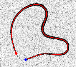


Fig. 6 illustrates a geodesic path computed using the curvature prior elastica model, where the curvature prior term is estimated pointwise from a given smooth curve as described in Eq. 24, and the cost function is constant. The given reference curve is shown on Fig. 6a, and connects an endpoint to another one , with tangent directions and shown as red and blue arrows respectively. The blue solid line in Fig. 6b illustrates the physical projection of the geodesic path obtained using the variant of the elastica model, equipped with the estimated curvature prior map described above, from the source point to the target point . In Fig. 6b, the reference smooth curve is shown in red and dashed. When the curvature penalization parameter is sufficiently large, as in this experiment where we use , the physical projection of the computed geodesic path should be almost overlaid onto the reference smooth curve, since they have almost identical curvature (recall that by construction the energy functional penalizes the square of their curvature difference), and since they share their endpoints and tangents at these endpoints. More precisely, the physical projection of the computed geodesic path converges to the reference curve as , and to a straight line joining the endpoints as . The computed geodesic path shown in Fig. 6b indeed well approximates the given reference curve, illustrating the effectiveness of the curvature prior in the considered variant of the classical elastica model.
5.1 Qualitative Comparison
In Fig. 7, we compare results obtained with the classical elastica model, and with the curvature prior elastica model, on five synthetic images. A common feature for the curvilinear structures in those images is that each of them involves strongly bent segments. The first column of Fig. 7 shows the initialization information for each synthetic image, where the blue and red dots together with the arrows stand for the source and target points respectively used to define the sets and . Columns and illustrate the physical projections of the computed geodesic paths from the classical elastica model and the curvature prior elastica model, respectively. More specifically, in column of rows to , we can observe that the physical projections of the geodesic paths from the classical elastica model are trapped into a shortcut problem, i.e. the projected paths travel along non-target regions. The reason is that the “correct” path features strongly curved segments whose squared curvature accumulate and lead to a high value of the classical elastica energy, hence it is not selected by this model. In contrast, in column of the same rows, the curvature prior elastica model indeed leads to accurate extraction of the target structures, even through the two endpoints of the structures in rows and are very close to each other. In rows and , each of the curvilinear structures is interrupted by an almost straight segment with slightly stronger appearance features, i.e. with higher values of the orientation score along this segment, yielding challenging crossing structures. In these tests, the physical projections of the geodesic paths from the classical elastica model pass through the interrupting segments, yielding a short branches combination problem (chen2018minimal), i.e. the obtained geodesic paths travel different segments not belonging to the targets. In contrast, the curvature prior elastica model produces satisfactory results which are able to accurately delineate the target curvilinear structures, as shown in column .


Fundus vessel tracking is a task of fundamental importance in retinal imaging and the relevant disease diagnosis. In Fig. 8, we compare the curvature prior elastica model to the classical elastica model in patches of retinal fundus images, chosen from the IOSTAR dataset (Zhang et al, 2016). In this experiment, the goal is to extract artery blood vessels, given two endpoints of each target vessel, as shown in the left column of Fig. 8. In a typical retinal fundus image, the major artery vessels usually exhibit weaker appearance features than those of the nearby vein vessels, and often cross over vein vessels yielding junction structures. An additional difficulty is that the target artery vessels also consist of segments with strong tortuosity. For the classical Euler-Mumford elastica model, one needs to assign a low importance weight to the curvature term, in order to avoid the underlying shortcut problem at those segments. However, this in turn encourages the computed paths to pass through the stronger neighboring vein vessels (whose cost is lower), thus increasing the risk of the short branches combination problem, see the center column of Fig. 8. In contrast, the minimization of the energy (16) defining the curvature prior elastica model favors optimal geodesic paths whose curvature is close to , allowing to handle scenarios where challenging structures such as crossings and strongly bent segments appear, see the right column of Fig. 8.
Another practical application for geodesic models is road tracking from aerial images, as demonstrated in Fig. 9. In this experiment, the centerlines of the objective roads have high Euclidean length, and simultaneously feature segments with low turning radii, as shown in Fig. 9a. We can see that the classical elastica model generates tracking results which suffer from a shortcut problem, see the center column of Fig. 9. In contrast, accurate results derived from the curvature prior elastica model are observed in the right column of Fig. 9, thanks to the use of the curvature prior term which alleviates difficulties associated to the complex scenarios.
| Elastica Model | Curvature Prior Elastica Model | |||||
|---|---|---|---|---|---|---|
| Ave. | Std. | Ave. | Std. | |||
5.2 Quantitative Comparison
We perform a quantitative evaluation of the performance and stability of the classical elastica model and of the curvature prior elastica model on synthetic images, when one varies the parameters and involved in these models, see Eqs. (16) and (25). These parameters determine the balance between the image data and the curvature regularization. The test data are generated by incorporating different levels of additive Gaussian noise to the original binary images of those shown in Fig. 7. More specifically, we add zero-mean Gaussian noise with levels of normalized variance values between and to each clean image, producing test images. Both geodesic models are configured by choosing parameters and , thus yielding runs per test image. In each test, the accuracy of the curvilinear structure tracking is measured using the Jaccard score between two bounded regions , defined as
| (27) |
where represents the area of the region . In our case, the regions and are defined as tubular neighborhoods with a fixed radius of grid points along the ground truth centerline and the physical projection of the computed geodesic path, respectively. Table 1 shows the quantitative results comparing the classical elastica model and the curvature prior elastica model, in terms of the Jaccard score between the ground truth centerlines and the physical projections of geodesic paths, see (27). In each row of Table 1, the average (Ave.) and standard deviation (Std.) values of , which are derived from runs w.r.t. different values of the parameters and . Overall, the results from the classical Euler-Mumford elastica model in general exhibit low average values of , and large standard deviation, reflecting the fact that various shortcut and short branches combination problems occur in most of the tests. In contrast, we observe much higher average values of using the curvature prior elastica model, and a smaller standard deviation, illustrating its ability to accurately and robustly extract curvilinear structures in the presence of strongly bent segments and junctions.
6 Conclusion and Discussion
In this work, we present a nonlinear HJB PDE approach to numerically compute the curve which globally minimizes a variant of the classical Euler-Mumford elastica energy, involving a curvature prior enhancement. The main contributions include (i) the establishment of the explicit expression of the Hamiltonian of the curvature prior elastica model, in such way that globally optimal paths can be characterized using the HJB PDE framework, (ii) the design of a finite differences scheme based on the HFM method for estimating the numerical solution to the associated HJB PDE, and (iii) the introduction of an efficient and robust method for computing the curvature prior in the context of curvilinear structure tracking. Numerical experiments indeed demonstrate promising results in medical and aerial images.
From the modeling standpoint, rather than penalizing the difference to a given curvature prior as proposed here, an alternative interesting route would be to penalize the variation of curvature along the path. The latter approach indeed appears to be appropriate and reasonable in relevant applications; for instance it would naturally address the shortcut problem, a segmentation artefact which usually involves sharp turns. For that purpose, one may for instance introduce in the elastica energy defined in (15) the squared derivative of the path curvature. However, this defines a third-order geodesic model, which raises substantial numerical difficulties. A closely related problem considered in the literature is the computation of geodesic paths with bounded derivative of curvature, however the approach Bakolas and Tsiotras (2009) cannot take into account a data-driven cost function, which is required by image processing applications. Another related problem is the penalization of torsion, a quantity which is also defined in terms of the third-order derivatives of the path, and is approximated in Ulen et al (2015) with the torsion of some local Bezier interpolations of the path. In the HJB PDE framework, considered in this paper, the computation of minimal geodesic paths for third-order planar models as considered here would involve the numerical solution of a strongly anisotropic PDE posed on the four dimensional domain , which implies an increased computational cost. We regard it as an opportunity for future research.
We have introduced a practical method for computing the curvature prior , using a set of reconstructed piecewise smooth centerlines which reflect the geometry of curvilinear structures in the image. In our work, those centerlines are numerically generated by applying a skeletonization procedure on the segmented curvilinear structures. A proper integration of the voting method Rouchdy and Cohen (2013) and of the keypoints detection method Benmansour and Cohen (2009); Kaul et al (2012) might be an alternative way for constructing the centerlines, where the dependency on the segmentation process can be removed. Furthermore, the estimation of the curvature of curves or surfaces from an orientation score map could also be investigated for computing , e.g. Bekkers et al (2015b). Unfortunately, the orientation score values around the positions where complex junctions appear usually lack reliability, thus requiring additional procedures to alleviate this problem.
We have established in Proposition 1 a general theoretical framework for deriving the Hamiltonian and control set of a curvature-penalized geodesic model equipped with a curvature prior enhancement, and have shown its application to the Euler-Mumford elastica model. This framework can also be exploited to generalize the Reeds-Sheep forward model Duits et al (2018) and the Dubins car model Mirebeau (2018). Finally, we intend to use the curvature-penalized geodesic models with curvature prior enhancement to address various image segmentation problems.
Appendix A Finite Difference Scheme for the Hamiltonian
We introduce here the numerical scheme for estimating the geodesic distance map associated to the Hamiltonian based on the state-of-the-art HFM method Mirebeau (2018, 2019). Recall that the distance map is the unique viscosity solution to the static HJB PDE
| (28) |
with the same point source and outflow boundary conditions as in (12). We discretize this PDE over the Cartesian grid
where is the grid scale, which is chosen so that is a positive integer for periodicity. Note that , where represents the number of angles discretized in the orientation dimension. We fix in the numerical experiments of this paper.
Given a non-zero vector and a relaxation parameter , a crucial ingredient of the HFM method Mirebeau (2018) is an approximation of the form
| (29) |
for any co-vector , where is a non-negative weight, and is an offset having integer coordinates, for each where is a positive integer. The construction of these weights and offsets relies on Selling’s decomposition of positive quadratic forms Mirebeau (2014b), with in dimension , and . In practice, we use .
By applying the approximation scheme in (29) to the terms of (21), we obtain the following expression
| (30) |
For the sake of readability, we leverage the abbreviations and to denote and , respectively. Combining (21) with (30) yields the following approximation of the Hamiltonian
| (31) |
The set of all offsets, at a given discretization point , is known as the stencil of the HFM method and defines the neighborhood system of this numerical scheme, see Fig. 10.


Now we can discretize the introduced Hamiltonian using a first order upwind finite difference scheme Mirebeau (2018)
| (32) |
for any discretization point and any offset . Since the offset has integer coordinates by construction, one has , and therefore the r.h.s. of (32) only involves values of the unknown geodesic distance map on the discretization grid . Finally, we obtain a finite differences discrete counterpart of the HJB PDE defined in (28)
| (33) |
for all , with boundary condition .
The HFM method computes the numerical solution to the discretized HJB PDE (see (33)) in an efficient single-pass wavefront propagation manner, using a generalization of the original Fast-Marching method Sethian (1999). Assuming that the computation is performed on a finite subset of the Cartesian grid , containing points, the computation complexity for estimating the solution to (33) is , where is the discretization parameter as used in (21), and as observed below (29). In practice, the choice is a good compromise between numerical accuracy and computation cost. Furthermore, the computation time of the HFM method can be deeply speeded up by exploiting a GPU-implemented scheme for estimating the geodesic distances, as proposed in (Mirebeau et al, 2023). The codes for the HFM method associated with the variant of the Euler-Mumford elastica model equipped with a curvature prior, involving the construction for the stencils, the computation for the geodesic distance map and the numerical solution to the geodesic backtracking ODE, can be downloaded from https://github.com/Mirebeau/HamiltonFastMarching.
References
- Bakolas and Tsiotras (2009) Bakolas E, Tsiotras P (2009) On the generation of nearly optimal, planar paths of bounded curvature and bounded curvature gradient. In: 2009 American Control Conference, 2009 American Control Conference, pp 385–390, DOI 10.1109/acc.2009.5160269
- Bardi and Capuzzo-Dolcetta (2008) Bardi M, Capuzzo-Dolcetta I (2008) Optimal control and viscosity solutions of Hamilton-Jacobi-Bellman equations. Birkhäuser Boston, MA, DOI 10.1007/978-0-8176-4755-1
- Bekkers et al (2014) Bekkers E, Duits R, Berendschot T, ter Haar Romeny B (2014) A multi-orientation analysis approach to retinal vessel tracking. Journal of Mathematical Imaging and Vision 49:583–610
- Bekkers et al (2015a) Bekkers EJ, Duits R, Mashtakov A, Sanguinetti GR (2015a) A PDE approach to data-driven sub-Riemannian geodesics in SE(2). SIAM J Imag Sci 8(4):2740–2770
- Bekkers et al (2015b) Bekkers EJ, Zhang J, Duits R, ter Haar Romeny BM (2015b) Curvature based biomarkers for diabetic retinopathy via exponential curve fits in se (2). In: Proc. Ophthalmic Medical Image Analysis International Workshop, University of Iowa, vol 2
- Bekkers et al (2018) Bekkers EJ, Chen D, Portegies JM (2018) Nilpotent approximations of sub-Riemannian distances for fast perceptual grouping of blood vessels in 2D and 3D. J Math Imag Vis 60(6):882–899
- Ben-Shahar and Ben-Yosef (2014) Ben-Shahar O, Ben-Yosef G (2014) Tangent bundle elastica and computer vision. IEEE Trans Pattern Anal Mach Intell 37(1):161–174
- Benmansour and Cohen (2009) Benmansour F, Cohen LD (2009) Fast object segmentation by growing minimal paths from a single point on 2D or 3D images. J Math Imaging Vis 33(2):209–221
- Benmansour and Cohen (2011) Benmansour F, Cohen LD (2011) Tubular structure segmentation based on minimal path method and anisotropic enhancement. Int J Comput Vis 92(2):192–210
- Caselles et al (1997) Caselles V, Kimmel R, Sapiro G (1997) Geodesic active contours. Int J Comput Vis 22(1):61–79
- Cetin et al (2012) Cetin S, Demir A, Yezzi A, Degertekin M, Unal G (2012) Vessel tractography using an intensity based tensor model with branch detection. IEEE Trans Med Imag 32(2):348–363
- Chambolle and Pock (2019) Chambolle A, Pock T (2019) Total roto-translational variation. Numer Math 142(3):611–666
- Chen et al (2016) Chen D, Mirebeau JM, Cohen LD (2016) Finsler geodesics evolution model for region based active contours. In: Proc. BMVC
- Chen et al (2017) Chen D, Mirebeau JM, Cohen LD (2017) Global minimum for a Finsler elastica minimal path approach. Int J Comput Vis 122(3):458–483
- Chen et al (2019) Chen D, Zhang J, Cohen LD (2019) Minimal paths for tubular structure segmentation with coherence penalty and adaptive anisotropy. IEEE Trans Image Process 28(3):1271–1284
- Chen et al (2021) Chen D, Cohen LD, Mirebeau JM, Tai XC (2021) An elastica geodesic approach with convexity shape prior. In: Proc. ICCV, pp 6900–6909
- Cohen and Kimmel (1997) Cohen LD, Kimmel R (1997) Global minimum for active contour models: A minimal path approach. Int J Comput Vis 24(1):57–78
- Dijkstra (1959) Dijkstra EW (1959) A note on two problems in connexion with graphs. Numer Math 1(1):269–271
- Duits et al (2018) Duits R, Meesters SP, Mirebeau JM, Portegies JM (2018) Optimal paths for variants of the 2D and 3D Reeds–Shepp car with applications in image analysis. J Math Imag Vis 60(6):816–848
- Franceschiello et al (2019) Franceschiello B, Mashtakov A, Citti G, Sarti A (2019) Geometrical optical illusion via sub-riemannian geodesics in the roto-translation group. Differ Geom Appl 65:55–77
- Franken and Duits (2009) Franken E, Duits R (2009) Crossing-preserving coherence-enhancing diffusion on invertible orientation scores. Int J Comput Vis 85:253–278
- Hummel and Zucker (1983) Hummel RA, Zucker SW (1983) On the foundations of relaxation labeling processes. IEEE Trans Pattern Anal Mach Intell (3):267–287
- Jbabdi et al (2008) Jbabdi S, Bellec P, Toro R, Daunizeau J, Pélégrini-Issac M, Benali H (2008) Accurate anisotropic fast marching for diffusion-based geodesic tractography. Int J Biomed Imaging 2008:2
- Kaul et al (2012) Kaul V, Yezzi A, Tsai Y (2012) Detecting curves with unknown endpoints and arbitrary topology using minimal paths. IEEE Trans Pattern Anal Mach Intell 34(10):1952–1965
- Kimmel and Sethian (2001) Kimmel R, Sethian JA (2001) Optimal algorithm for shape from shading and path planning. J Math Imaging Vis 14:237–244
- Kimmel et al (1995) Kimmel R, Shaked D, Kiryati N, Bruckstein AM (1995) Skeletonization via distance maps and level sets. Comput Vis Image Underst 62(3):382–391
- Lam et al (1992) Lam L, Lee SW, Suen CY (1992) Thinning methodologies-A comprehensive survey. IEEE Trans Pattern Anal Mach Intell 14(09):869–885
- Law and Chung (2008) Law MWK, Chung ACS (2008) Three Dimensional Curvilinear Structure Detection Using Optimally Oriented Flux. In: Proc. ECCV, pp 368–382
- Li and Yezzi (2007) Li H, Yezzi A (2007) Vessels as 4-D curves: Global minimal 4-D paths to extract 3-D tubular surfaces and centerlines. IEEE Trans Med Imag 26(9):1213–1223
- Liao et al (2018) Liao W, Wörz S, Kang CK, Cho ZH, Rohr K (2018) Progressive minimal path method for segmentation of 2D and 3D line structures. IEEE Trans Pattern Anal Mach Intell 40(3):696–709
- Melonakos et al (2008) Melonakos J, Pichon E, Angenent S, Tannenbaum A (2008) Finsler active contours. IEEE Trans Pattern Anal Mach Intell 30(3):412–423
- Mirebeau (2014a) Mirebeau JM (2014a) Anisotropic fast-marching on cartesian grids using lattice basis reduction. SIAM J Numer Anal 52(4):1573–1599
- Mirebeau (2014b) Mirebeau JM (2014b) Efficient fast marching with Finsler metrics. Numer Math 126(3):515–557
- Mirebeau (2018) Mirebeau JM (2018) Fast-marching methods for curvature penalized shortest paths. J Math Imag Vis 60(6):784–815
- Mirebeau (2019) Mirebeau JM (2019) Riemannian fast-marching on Cartesian grids, using Voronoi’s first reduction of quadratic forms. SIAM J Numer Anal 57(6):2608–2655
- Mirebeau and Portegies (2019) Mirebeau JM, Portegies J (2019) Hamiltonian fast marching: A numerical solver for anisotropic and non-holonomic eikonal pdes. Image Processing On Line 9:47–93
- Mirebeau et al (2023) Mirebeau JM, Gayraud L, Barrère R, Chen D, Desquilbet F (2023) Massively parallel computation of globally optimal shortest paths with curvature penalization. Concurrency Computat, Pract Exper 35(2):e7472
- Mumford (1994) Mumford D (1994) Elastica and computer vision. in Algebraic Geometry and Its Applications (C. L. Bajaj, Ed.), Springer-Verlag, New York, pages 491-506
- Mumford and Shah (1989) Mumford D, Shah J (1989) Optimal approximations by piecewise smooth functions and associated variational problems. Commun Pure Appl Math 42(5):577–685
- Nitzberg (1990) Nitzberg D M Mumford (1990) The 2.1-D Sketch*. In: Proc. ICCV, pp 138–144
- Parent and Zucker (1989) Parent P, Zucker SW (1989) Trace inference, curvature consistency, and curve detection. IEEE Trans Pattern Anal Mach Intell 11(8):823–839
- Parker et al (2002) Parker GJ, Wheeler-Kingshott CA, Barker GJ (2002) Estimating distributed anatomical connectivity using fast marching methods and diffusion tensor imaging. IEEE Trans Med Imag 21(5):505–512
- Péchaud et al (2009) Péchaud M, Keriven R, Peyré G (2009) Extraction of tubular structures over an orientation domain. In: Proc. CVPR, pp 336–342
- Peyré et al (2010) Peyré G, Péchaud M, Keriven R, Cohen LD (2010) Geodesic methods in computer vision and graphics. Foundations and Trends in Computer Graphics and Vision 5(3–4):197–397
- Randers (1941) Randers G (1941) On an asymmetrical metric in the four-space of general relativity. Phys Rev 59(2):195
- Rouchdy and Cohen (2013) Rouchdy Y, Cohen LD (2013) Geodesic voting for the automatic extraction of tree structures. Methods and applications. Comput Vis Image Underst 117(10):1453–1467
- Saye and Sethian (2012) Saye R, Sethian JA (2012) Analysis and applications of the Voronoi implicit interface method. J Comput Phys 231(18):6051–6085
- Saye and Sethian (2011) Saye RI, Sethian JA (2011) The voronoi implicit interface method for computing multiphase physics. Proc Nat Acad Sci 108(49):19,498–19,503
- Sethian (1996) Sethian JA (1996) A fast marching level set method for monotonically advancing fronts. Proc Nat Acad Sci 93(4):1591–1595
- Sethian (1999) Sethian JA (1999) Fast marching methods. SIAM Review 41(2):199–235
- Sethian and Vladimirsky (2001) Sethian JA, Vladimirsky A (2001) Ordered upwind methods for static Hamilton–Jacobi equations. Proc Nat Acad Sci 98(20):11,069–11,074
- Sethian and Vladimirsky (2003) Sethian JA, Vladimirsky A (2003) Ordered upwind methods for static Hamilton–Jacobi equations: Theory and algorithms. SIAM J Numer Anal 41(1):325–363
- Siddiqi et al (2002) Siddiqi K, Bouix S, Tannenbaum A, Zucker SW (2002) Hamilton-jacobi skeletons. Int J Comput Vis 48(3):215–231
- Türetken et al (2016) Türetken E, Benmansour F, Andres B, Głowacki P, Pfister H, Fua P (2016) Reconstructing curvilinear networks using path classifiers and integer programming. IEEE Trans Pattern Anal Mach Intell 38(12):2515–2530
- Ulen et al (2015) Ulen J, Strandmark P, Kahl F (2015) Shortest paths with higher-order regularization. IEEE Trans Pattern Anal Mach Intell 37(12):2588–2600
- Wertheimer (1938) Wertheimer M (1938) Laws of organization in perceptual forms (partial translation). In: A sourcebook of Gestalt Psychology, Kegan Paul, Trench, Trubner & Company, pp 71–88
- Zhang et al (2016) Zhang J, Dashtbozorg B, Bekkers E, Pluim JP, Duits R, ter Haar Romeny BM (2016) Robust retinal vessel segmentation via locally adaptive derivative frames in orientation scores. IEEE Trans Med Imag 35(12):2631–2644