Computing the nc-rank via discrete convex optimization on CAT(0) spaces

Masaki HAMADA and Hiroshi HIRAI
Department of Mathematical Informatics,
Graduate School of Information Science and Technology,
The University of Tokyo, Tokyo, 113-8656, Japan.
masaki

\_

hamada@mist.i.u-tokyo.ac.jp
hirai@mist.i.u-tokyo.ac.jp

Abstract

In this paper, we address the noncommutative rank (nc-rank) computation of a linear symbolic matrix

A=A_{1}x_{1}+A_{2}x_{2}+\cdots+A_{m}x_{m},

where each $A_{i}$ is an $n\times n$ matrix over a field ${\mathbb{K}}$ , and $x_{i}$ $(i=1,2,\ldots,m)$ are noncommutative variables. For this problem, polynomial time algorithms were given by Garg, Gurvits, Oliveira, and Wigderson for ${\mathbb{K}}={\mathbb{Q}}$ , and by Ivanyos, Qiao, and Subrahmanyam for an arbitrary field ${\mathbb{K}}$ . We present a significantly different polynomial time algorithm that works on an arbitrary field ${\mathbb{K}}$ . Our algorithm is based on a combination of submodular optimization on modular lattices and convex optimization on CAT(0) spaces.

Keywords: Edmonds’ problem, noncommutative rank, CAT(0) space, proximal point algorithm, submodular function, modular lattice, $p$ -adic valuation, Euclidean building

1 Introduction

The present article addresses rank computation of a linear symbolic matrix— a matrix of the following form:

A=A_{1}x_{1}+A_{2}x_{2}+\cdots+A_{m}x_{m},

(1.1)

where each $A_{i}$ is an $n\times n$ matrix over a field ${\mathbb{K}}$ , $x_{i}$ $(i=1,2,\ldots,m)$ are variables, and $A$ is viewed as a matrix over ${\mathbb{K}}(x_{1},x_{2},\ldots,x_{m})$ . This problem, sometimes called Edmonds’ problem, has fundamental importance in a wide range of applied mathematics and computer science; see [36]. Edmonds’ problem (on large field ${\mathbb{K}}$ ) is a representative problem that belongs to RP—the class of problems having a randomized polynomial time algorithm—but is not known to belong to P. The existence of a deterministic polynomial time algorithm for Edmonds’ problem is one of the major open problems in theoretical computer science.

In 2015, Ivanyos, Qiao, and Subrahmanyam [29] introduced a noncommutative formulation of the Edmonds’ problem, called the noncommutative Edmonds’ problem. In this formulation, linear symbolic matrix $A$ is regarded as a matrix over the free skew field ${\mathbb{K}}(\langle x_{1},\ldots,x_{m}\rangle)$ , which is the “most generic” skew field of fractions of noncommutative polynomial ring ${\mathbb{K}}\langle x_{1},\ldots,x_{m}\rangle$ . The rank of $A$ over the free skew field is called the noncommutative rank, or nc-rank, which is denoted by $\mathop{\rm nc\mbox{-}rank}A$ . Contrary to the commutative case, the noncommutative Edmonds’ problem can be solved in polynomial time.

Theorem 1.1 ([17, 30]).

The nc-rank of a matrix $A$ of form (1.1) can be computed in polynomial time.

As well as the result, the algorithms for nc-rank are stimulating subsequent researches. The first polynomial time algorithm is due to Garg, Gurvits, Oliveira, and Wigderson [17] for the case of ${\mathbb{K}}={\mathbb{Q}}$ . They showed that Gurvits’ operator scaling algorithm [19], which was designed for solving a special class (Edmonds-Rado class) of Edmonds’ problem, can solve nc-singularity testing (i.e., testing whether $n=\mathop{\rm nc\mbox{-}rank}A$ ) in polynomial time. The operator scaling algorithm has rich connections to various fields of mathematical sciences. Particularly, nc-singularity testing can be formulated as a geodesically-convex optimization problem on Riemannian manifold $GL_{n}({\mathbb{R}})/O_{n}({\mathbb{R}})$ , and the operator scaling can be viewed as a minimization algorithm on it; see [2]. For explosive developments after [17], we refer to e.g., [9] and the references therein.

Ivanyos, Qiao, and Subrahmanyam [29, 30] developed the first polynomial time algorithm for the nc-rank that works on an arbitrary field ${\mathbb{K}}$ . Their algorithm is viewed as a “vector-space generalization” of the augmenting path algorithm in the bipartite matching problem. This indicates a new direction in combinatorial optimization, since Edmonds’ problem generalizes several important combinatorial optimization problems. Inspired by their algorithm, [27] developed a combinatorial polynomial time algorithm for a certain algebraically constraint 2-matching problem in a bipartite graph, which corresponds to the (commutative) Edmonds’ problem for a linear symbolic matrix in [32]. Also, a noncommutative algebraic formulation that captures weighted versions of combinatorial optimization problems was studied in [25, 26, 40].

The main contribution of this paper is a significantly different polynomial time algorithm for computing the nc-rank on an arbitrary field ${\mathbb{K}}$ . While describing the above algorithms and validity proofs is rather tough work, the algorithm and proof presented in this paper are conceptually simple, elementary, and relatively short. Further, it is also relevant to the following two cutting edge issues in discrete and continuous optimization:

•

submodular optimization on a modular lattice.
•

convex optimization on a CAT(0) space.

A submodular function $f$ on a lattice ${\cal L}$ is a function $f:{\cal L}\to{\mathbb{R}}$ satisfying $f(p)+f(q)\geq f(p\vee q)+f(p\wedge q)$ for $p,q\in{\cal L}$ . Submodular functions on Boolean lattice $\{0,1\}^{n}$ are well-studied, and have played central roles in the developments of combinatorial optimization; see [15]. They are correspondents of convex functions (discrete convex functions) in discrete optimization; see [37]. Optimization of submodular functions beyond Boolean lattices, particularly on modular lattices, is a new research area that has just started; see [16, 24, 34] on this subject.

A CAT(0) space is a (non-manifold) generalization of nonpositively curved Riemannian manifolds; see [8]. While CAT(0) spaces have been studied mainly in geometric group theory, their effective utilization in applied mathematics has gained attention; see e.g.,[6]. A CAT(0) space is a uniquely-geodesic metric space, and convexity concepts are defined along unique geodesics. Theory of algorithms and optimization on CAT(0) spaces is now being pioneered; see e.g., [3, 4, 5, 22, 41].

Our algorithm is obtained as a combination of these new optimization approaches. We hope that this will bring new interactions to the nc-rank literature. While it is somehow relevant to geodesically-convex optimization mentioned above, we deal with optimization on combinatorially-defined non-manifold CAT(0) spaces. The most important implication of our result is that convex optimization algorithms on such spaces can be a tool of showing polynomial time complexity.

Outline.

Let us outline our algorithm. As shown by Fortin and Reutenauer [14], the nc-rank is given by the optimum value of an optimization problem:

Theorem 1.2 ([14]).

Let $A$ be a matrix of form (1.1). Then $\mathop{\rm nc\mbox{-}rank}A$ is equal to the optimal value of the following problem:

	$\displaystyle{\rm FR}:\quad{\rm Min.}$		$\displaystyle 2n-r-s$
	$\displaystyle{\rm s.t.}$		$SAT$ has an $r\times s$ zero submatrix,
			$\displaystyle S,T\in GL_{n}({\mathbb{K}}).$

As in [29, 30], our algorithm is designed to solve this optimization problem. This problem FR can also be formulated as an optimization problem on the modular lattice of vector subspaces in ${\mathbb{K}}^{n}$ , as follows. Regard each matrix $A_{i}$ as a bilinear form ${\mathbb{K}}^{n}\times{\mathbb{K}}^{n}\to{\mathbb{K}}$ by

A_{i}(x,y):=x^{\top}A_{i}y\quad(x,y\in{\mathbb{K}}^{n}).

Then the condition of FR says that there is a pair of vector subspaces $U$ and $V$ of dimension $r$ and $s$ , respectively, that annihilates all bilinear forms, i.e., $A_{i}(U,V):=\{0\}$ . The objective function is written as $2n-\dim U-\dim V$ . Therefore, FR is equivalent to the following problem (maximum vanishing subspace problem; MVSP):

	$\displaystyle{\rm MVSP}:\quad{\rm Min.}$		$\displaystyle-\dim X-\dim Y$
	$\displaystyle{\rm s.t.}$		$\displaystyle A_{i}(X,Y)=\{0\}\quad(i=1,2,\ldots,m),$
			$\displaystyle X,Y:\mbox{vector subspaces of ${\mathbb{K}}^{n}$}.$

It is a basic fact that the family ${\cal L}$ of all vector subspaces in $\mathbb{K}^{n}$ forms a modular lattice with respect to the inclusion order. Hence, MVSP is an optimization problem over ${\cal L}\times{\cal L}$ . Further, by reversing the order of the second ${\cal L}$ , it can be viewed as a submodular function minimization (SFM) on modular lattice ${\cal L}\times{\cal L}$ ; see Proposition 3.2 in Section 3.1.

Contrary to the Boolean case, it is not known generally whether a submodular function on a modular lattice can be minimized in polynomial time. The reason of polynomial-time solvability of SFM on Boolean lattice $\{0,1\}^{n}$ is the Lovász extension [35]— a piecewise-linear interpolation $\bar{f}:[0,1]^{n}\to{\mathbb{R}}$ of function $f:\{0,1\}^{n}\to{\mathbb{R}}$ such that $\bar{f}$ is convex if and only if $f$ is submodular. For SFM on a modular lattice, however, such a good convex relaxation to $\mathbb{R}^{n}$ is not known.

A recent study [24] introduced an approach of constructing a convex relaxation of SFM on a modular lattice, where the domain of the relaxation is a CAT(0) space. The construction is based on the concept of an orthoscheme complex [7]. Consider the order complex $K({\cal L})$ of ${\cal L}$ , and endow each simplex with a specific Euclidean metric. The resulting metric space $K({\cal L})$ is called the orthoscheme complex of ${\cal L}$ , and is dealt with as a continuous relaxation of ${\cal L}$ . The details are given in Section 2.2.2. Figure 1 illustrates the orthoscheme complex of a modular lattice with rank $2$ , which is obtained by gluing Euclidean isosceles right triangles along longer edges.

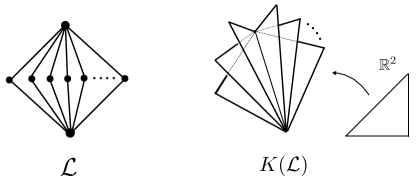
Refer to caption — Figure 1: An orthoscheme complex

The orthoscheme complex of a modular lattice was shown to be CAT(0) [10]. This enables us to consider geodesically-convexity for functions on $K({\cal L})$ . In this setting, a submodular function $f:{\cal L}\to{\mathbb{R}}$ is characterized by the convexity of its piecewise linear interpolation, i.e., Lovász extension $\bar{f}:K({\cal L})\to{\mathbb{R}}$ [24]. According to this construction, we obtain an exact convex relaxation of MVSP in a CAT(0)-space.

Our proposed algorithm is obtained by applying the splitting proximal point algorithm (SPPA) to this convex relaxation. SPPA is a generic algorithm that minimizes a convex function of a separable form $\sum_{i=1}^{N}f_{i}$ , where each $f_{i}$ is a convex function. Each iteration of the algorithm updates the current point $x$ to its resolvent of $f_{i}$ — a minimizer of $y\mapsto f_{i}(y)+(1/\lambda)d(y,x)^{2}$ , where $i$ is chosen cyclically. Bačák [4] showed that SPPA generates a sequence convergent to a minimizer of $f$ (under a mild assumption). Subsequently, Ohta and Pálfia [39] proved a sublinear convergence of SPPA.

The main technical contribution is to show that SPPA is applicable to the convex relaxation of MVSP and becomes a polynomial time algorithm for MVSP: We provide an equivalent convex relaxation of MVSP with a separable objective function $\sum_{i}f_{i}$ , and show that the resolvent of each $f_{i}$ can be computed in polynomial time. By utilizing the sublinear convergence estimate, a polynomial number of iterations for SPPA identifies an optimal solution of MVSP.

Compared with the existing algorithms, this algorithm has advantages and drawbacks. As mentioned above, our algorithm and its validity proof are relatively simple. Particularly, it can be uniformly written for an arbitrary field ${\mathbb{K}}$ , where only the requirement for ${\mathbb{K}}$ is that arithmetic operations is executable. No care is needed for a small finite field, whereas the algorithm in [29, 30] needs a field extension. On the other hand, our algorithm is very slow; see Theorem 3.3. This is caused by using a generic and primitive algorithm (SPPA) for optimization on CAT(0) spaces. We believe that this will be naturally improved in future developments.

The problematic point of our algorithm is bit-complexity explosion for the case of ${\mathbb{K}}={\mathbb{Q}}$ . Our algorithm updates feasible vector subspaces in MVSP, and can cause an exponential increase of the bit-size representing bases of those vector subspaces. To resolve this problem and make use of the advantage in finite fields, we propose a reduction of nc-rank computation on ${\mathbb{Q}}$ to that on $GF(p)$ . This reduction is an application of the $p$ -adic valuation on ${\mathbb{Q}}$ . We consider a weighted version of the nc-rank, which was introduced by [25] for ${\mathbb{K}}(t)$ and is definable for an arbitrary field with a discrete valuation. The corresponding optimization problem MVMP is a discrete convex optimization on a representative CAT(0) space—the Euclidean building for $GL_{n}({\mathbb{Q}})$ (or $GL_{n}({\mathbb{Q}}_{p})$ ). This may be viewed as a $p$ -adic counterpart of the above geodesically-convex optimization approach on $GL_{n}({\mathbb{R}})/O_{n}({\mathbb{R}})$ for nc-singularity testing on ${\mathbb{Q}}$ . By using an obvious relation of the $p$ -adic valuation of a nonzero integer and its bit-length in base $p$ , we show that nc-singularity testing on ${\mathbb{Q}}$ reduces to a polynomial number of nc-rank computation over the residue field $GF(p)$ , in which the required bit-length is polynomially bounded.

Organization.

The rest of this paper is organized as follows. In Section 2, we present necessary backgrounds on convex optimization on CAT(0) space, modular lattices, and submodular functions. In Section 3, we present our algorithm and show its validity. In Section 4, we present the $p$ -adic reduction for nc-rank computation on ${\mathbb{Q}}$ .

Original motivation: Block triangularization of a partitioned matrix.

The original version [21] of this paper dealt with block triangularization of a matrix with the following partition structure:

A=\left(\begin{array}[]{ccccc}A_{11}&A_{12}&\cdots&A_{1\nu}\\ A_{21}&A_{22}&\cdots&A_{2\nu}\\ \vdots&\vdots&\ddots&\vdots\\ A_{\mu 1}&A_{\mu 2}&\cdots&A_{\mu\nu}\end{array}\right),

where $A_{\alpha\beta}$ is an $n_{\alpha}\times m_{\beta}$ matrix over field ${\mathbb{K}}$ for $\alpha\in[\mu]$ and $\beta\in[\nu]$ . Consider the following block triangularization

A\mapsto PEAFQ=\left[\begin{array}[]{ccccc}\vrule\lx@intercol\hfil\hfil\lx@intercol&&&\\ \cline{1-1}\cr&\vrule\lx@intercol\hfil\hfil\lx@intercol&&\text{\huge$*$}\\ \cline{2-3}\cr&&&\vrule\lx@intercol\hfil\hfil\lx@intercol&\\ \cline{4-4}\cr\text{\huge$O$}&&&&\vrule\lx@intercol\hfil\hfil\lx@intercol\\ \cline{5-5}\cr\end{array}\right],

where $P$ and $Q$ are permutation matrices and $E$ and $F$ are regular transformations “within blocks,” i.e., $E$ and $F$ are block diagonal matrices with block diagonals $E_{\alpha}\in GL_{n_{\alpha}}({\mathbb{K}})$ $(\alpha\in[\mu])$ and $F_{\beta}\in GL_{m_{\beta}}({\mathbb{K}})$ $(\beta\in[\mu])$ , respectively. Such a block triangularization was addressed by Ito, Iwata, and Murota [31] for motivating analysis on physical systems with (restricted) symmetry. The most effective block triangularization is determined by arranging a maximal chain of maximum-size zero-blocks exposed in $EAF$ , where the size of a zero block is defined as the sum of row and column numbers. This generalizes the classical Dulmage-Mendelsohn decomposition for bipartite graphs and Murota’s combinatorial canonical form for layered mixed matrices; see [23, 37].

Finding a maximum-size zero-block is nothing but FR (or MVSP) for the linear symbolic matrix obtained by multiplying variable $x_{\alpha\beta}$ to $A_{\alpha\beta}$ ; see [25, Appendix] for details. The original version of our algorithm was designed for this zero-block finding. Later, we found that this is essentially nc-rank computation. This new version improves analysis (on Theorem 3.3), simplifies the arguments, particularly the proof of Theorem 3.9, and includes the new section for the $p$ -adic reduction.

2 Preliminaries

Let $[n]$ denote $\{1,2,\ldots,n\}$ . Let ${\mathbb{R}}$ , ${\mathbb{Q}}$ , ${\mathbb{Z}}$ denote the sets of real, rational, and integer numbers, respectively. Let $1_{X}$ denote the vector in ${\mathbb{R}}^{n}$ such that $(1_{X})_{i}=1$ if $i\in X$ and zero otherwise. The $i$ -unit vector $1_{\{i\}}$ is simply written as $1_{i}$ .

2.1 Convex optimization on CAT(0)-spaces

2.1.1 CAT(0)-spaces

Let $K$ be a metric space with distance function $d$ . A path in $K$ is a continuous map $\gamma:[0,1]\to L$ , where its length is defined as $\sup\sum_{i=0}^{N-1}d(\gamma(t_{i}),\gamma(t_{i+1}))$ over $0=t_{0}<t_{1}<t_{2}<\cdots<t_{N}=1$ and $N>0$ . If $\gamma(0)=x$ and $\gamma(1)=y$ , then we say that a path $\gamma$ connects $x,y$ . A geodesic is a path $\gamma$ satisfying $d(\gamma(s),\gamma(t))=d(\gamma(0),\gamma(1))|s-t|$ for every $s,t\in[0,1]$ . A geodesic metric space is a metric space $K$ in which any pair of two points is connected by a geodesic. Additionally, if a geodesic connecting any points is unique, then $K$ is called uniquely geodesic.

We next introduce a CAT(0) space. Informally, it is defined as a geodesic metric space in which any triangle is not thicker than the corresponding triangle in Euclidean plane. We here adopt the following definition. A geodesic metric space $K$ is said to be CAT(0) if for every point $x\in K$ , every geodesic $\gamma:[0,1]\to K$ and $t\in[0,1]$ , it holds

d(x,\gamma(t))^{2}\leq(1-t)d(x,\gamma(0))^{2}+td(x,\gamma(1))^{2}-t(1-t)d(\gamma(0),\gamma(1))^{2}.

(2.1)

The following property of a CAT(0) space is a basis of introducing convexity.

Proposition 2.1 ([8, Proposition 1.4]).

A CAT $(0)$ -space is uniquely geodesic.

Suppose that $K$ is a CAT $(0)$ space. For points $x,y$ in $K$ , let $[x,y]$ denote the image of a unique geodesic $\gamma$ connecting $x,y$ . For $t\in[0,1]$ , the point $p$ on $[x,y]$ with $d(x,p)/d(x,y)=t$ is formally written as $(1-t)x+ty$ .

A function $f:K\to{\mathbb{R}}$ is said to be convex if for all $x,y\in K,t\in[0,1]$ it satisfies

f((1-t)x+ty)\leq(1-t)f(x)+tf(y).

If it satisfies a stronger inequality

f((1-t)x+ty)\leq(1-t)f(x)+tf(y)-\frac{\kappa}{2}t(1-t)d(x,y)^{2}

for some $\kappa>0$ , then $f$ is said to be strongly convex with parameter $\kappa>0$ . In this paper, we always assume that a convex function is continuous. A function $f:K\to{\mathbb{R}}$ is said to be $L$ -Lipschitz with parameter $L\geq 0$ if for all $x,y\in K$ it satisfies

|f(x)-f(y)|\leq Ld(x,y).

Lemma 2.2.

For any $z\in K$ , the function $x\mapsto d(z,x)^{2}$ is strongly convex with parameter $\kappa=2$ , and is $L$ -Lipschitz with $L=2\mathop{\rm diam}K$ , where $\mathop{\rm diam}K:=\sup_{x,y\in K}d(x,y)$ denotes the diameter of $K$

The former follows directly from the definition (2.1) of CAT(0)-space. The latter follows from $d(z,x)^{2}-d(z,y)^{2}\leq(d(z,x)+d(z,y))(d(z,x)-d(z,y))=(d(z,x)+d(z,y))d(x,y)\leq(2\mathop{\rm diam}K)d(x,y)$ .

2.1.2 Proximal point algorithm

Let $K$ be a complete CAT(0)-space (which is also called an Hadamard space). For a convex function $f:K\to{\mathbb{R}}$ and $\lambda>0$ the resolvent of $f$ is a map $J_{\lambda}^{f}:K\to K$ defined by

J_{\lambda}^{f}(x):=\mathop{\rm argmin}_{y\in K}\left(f(y)+\frac{1}{2\lambda}d(x,y)^{2}\right)\quad(x\in K).

Since the function $y\mapsto f(y)+\frac{1}{2\lambda}d(x,y)^{2}$ is strongly convex with parameter $1/\lambda>0$ , the minimizer is uniquely determined, and $J_{\lambda}^{f}$ is well-defined; see [5, Proposition 2.2.17].

The proximal point algorithm (PPA) is to iterate updates $x\leftarrow J_{\lambda}^{f}(x)$ . This simple algorithm generates a sequence converging to a minimizer of $f$ under a mild assumption; see [3, 5]. The splitting proximal point algorithm (SPPA) [4, 5], which we will use, minimizes a convex function $f:K\to{\mathbb{R}}$ represented as the following form

f:=\sum_{i=1}^{m}f_{i},

where each $f_{i}:K\to{\mathbb{R}}$ is a convex function. Consider a sequence $(\lambda_{k})_{k=1,2,\ldots,}$ satisfying

\sum_{k=0}^{\infty}\lambda_{k}=\infty,\quad\sum_{k=0}^{\infty}\lambda_{k}^{2}<\infty.

Splitting Proximal Point Algorithm (SPPA)

$\bullet$

Let $x_{0}\in K$ be an initial point.

$\bullet$

For $k=0,1,2,\ldots$ , repeat the following:

x_{km+i}:=J_{\lambda_{k}}^{f_{i}}(x_{km+i-1})\quad(i=1,2,\ldots,m).

Bačák [4] showed that the sequence generated by SPPA converges to a minimizer of $f$ if $K$ is locally compact. Ohta and Pálfia [39] proved sublinear convergence of SPPA if $f$ is strongly convex and $K$ is not necessarily locally compact.

Theorem 2.3 ([39]).

Suppose that $f$ is strongly convex with parameter $\epsilon>0$ and each $f_{i}$ is $L$ -Lipschitz. Let $x^{*}$ be the unique minimizer of $f$ . Define the sequence $(\lambda_{k})$ by

\lambda_{k}:=1/\epsilon(k+1).

Then the sequence $(x_{\ell})$ generated by SPPA satisfies

d(x_{km},x^{*})^{2}=O\left(\frac{\log k}{k}\frac{L^{2}m^{2}}{\epsilon^{2}}\right)\quad(k=1,2,\ldots).

2.2 Geometry of modular lattices

We use basic terminologies and facts in lattice theory; see e.g., [18]. A lattice ${\cal L}$ is a partially ordered set in which every pair $p,q$ of elements has meet $p\wedge q$ (greatest common lower bound) and join $p\vee q$ (lowest common upper bound). Let $\preceq$ denote the partial order, where $p\prec q$ means $p\preceq q$ and $p\neq q$ . A pairwise comparable subset of ${\cal L}$ , arranged as $p_{0}\prec p_{1}\prec\cdots\prec p_{k}$ , is called a chain (from $p_{0}$ to $p_{k}$ ), where $k$ is called the length. In this paper, we only consider lattices in which any chain has a finite length. Let ${\bf 0}$ and ${\bf 1}$ denote the minimum and maximum elements of ${\cal L}$ , respectively. The rank $r(p)$ of element $p$ is defined as the maximum length of a chain from ${\bf 0}$ to $p$ . The rank of lattice ${\cal L}$ is defined as the rank of ${\bf 1}$ . For elements $p,q$ with $p\preceq q$ the interval $[p,q]$ is the set of elements $u$ with $p\preceq u\preceq q$ . Restricting $\preceq$ to $[p,q]$ , the interval $[p,q]$ is a lattice with maximum $q$ and minimum $p$ . If $p\neq q$ and $[p,q]=\{p,q\}$ , we say that $q$ covers $p$ and denote $p\prec:q$ or $q:\succ p$ . For two lattices ${\cal L},{\cal M}$ , their direct product ${\cal L}\times{\cal M}$ becomes a lattice, where the partial order on ${\cal L}\times{\cal M}$ is defined by $(p,p^{\prime})\preceq(q,q^{\prime})\Leftrightarrow p\preceq q,p^{\prime}\preceq q^{\prime}$ .

A lattice ${\cal L}$ is called modular if for every triple $x,a,b$ of elements with $x\preceq b$ , it holds $x\vee(a\wedge b)=(x\vee a)\wedge b$ . A modular lattice satisfies the Jordan-Dedekind chain condition. This is, the lengths of maximal chains of every interval are the same. Also, we often use the following property:

p\prec:p^{\prime}\ \Rightarrow\ p\wedge q=p^{\prime}\wedge q\ \ \mbox{or}\ \ p\wedge q\prec:p^{\prime}\wedge q.

(2.2)

This can be seen from the definition of modular lattices, and holds also when replacing $\wedge$ by $\vee$ .

A modular lattice ${\cal L}$ is said to be complemented if every element can be represented as a join of atoms, where an atom is an element of rank $1$ . It is known that for a complemented modular lattice, every interval is complemented modular, and a lattice obtained by reversing the partial order is also complemented modular. The product of two complemented modular lattices is also complemented modular.

A canonical example of a complemented modular lattice is the family ${\cal L}$ of all subspaces of a vector space $U$ , where the partial order is the inclusion order with $\wedge=\cap$ , and $\vee=+$ . Another important example is a Boolean lattice—a lattice isomorphic to the poset $2^{[n]}$ of all subsets of $[n]$ with respect to the inclusion order $\subseteq$ .

2.2.1 Frames—Boolean sublattices in a complemented modular lattice

Let ${\cal L}$ be a complemented modular lattice of rank $n$ , and let $r$ denote the rank function of ${\cal L}$ . A complemented modular lattice is equivalent to a spherical building of type A [1]. We consider a lattice-theoretic counterpart of an apartment, which is a maximal Boolean sublattice of ${\cal L}$ .

A base is a set of $n$ atoms $a_{1},a_{2},\ldots,a_{n}$ with $a_{1}\vee a_{2}\vee\cdots\vee a_{n}={\bf 1}$ . The sublattice $\langle a_{1},a_{2},\ldots,a_{n}\rangle$ generated by a base $\{a_{1},a_{2},\ldots,a_{n}\}$ is called a frame, which is isomorphic to a Boolean lattice $2^{[n]}$ by the map

X\mapsto\bigvee_{i\in X}a_{i}.

Lemma 2.4 (see e.g.,[18]).

Let ${\cal L}$ be a complemented modular lattice of rank $n$ .

(1)

For chains ${\cal C},{\cal D}$ in $\cal L$ , there is a frame ${\cal F}\subseteq{\cal L}$ containing $\cal C$ and $\cal D$ .

(2)

For a frame ${\cal F}$ and an ordering $a_{1},a_{2},\ldots,a_{n}$ of its basis, define map $\varphi_{a_{1},a_{2},\ldots,a_{n}}:{\cal L}\to{\cal F}$ by

p\mapsto\bigvee\{a_{i}\mid i\in[n]:p\wedge(a_{1}\vee a_{2}\vee\cdots\vee a_{i}):\succ p\wedge(a_{1}\vee a_{2}\vee\cdots\vee a_{i-1})\}.

(2.3)

Then $\varphi_{a_{1},a_{2},\ldots,a_{n}}$ is a retraction to ${\cal F}$ such that it is rank-preserving (i.e., $r(p)=r(\varphi(p))$ ) and order-preserving (i.e., $p\preceq q\Rightarrow\varphi(p)\preceq\varphi(q)$ ).

This is nothing but a part of the axiom of building, where the map in (2) is essentially a canonical retraction to an apartment.

Proof.

We show (1) by the induction on $n$ . Suppose that ${\cal C}=({\bf 0}=p_{0}\prec p_{1}\prec\cdots\prec p_{n}={\bf 1})$ and ${\cal D}=({\bf 0}=q_{0}\prec q_{1}\prec\cdots\prec q_{n}={\bf 1})$ . Consider the maximal chains ${\cal C}^{\prime},{\cal D}^{\prime}$ from ${\bf 0}$ to $p_{n-1}$ , where ${\cal C}^{\prime}:=({\bf 0}=p_{0}\prec p_{1}\prec\cdots\prec p_{n-1})$ and ${\cal D}^{\prime}$ consists of $q_{i}^{\prime}:=p_{n-1}\wedge q_{i}$ $(i=0,1,\ldots,n)$ . Note that the maximality of ${\cal D}^{\prime}$ follows from (2.2). By induction, there is a frame $\langle a_{1},a_{2},\ldots,a_{n-1}\rangle$ of the interval $[{\bf 0},p_{n-1}]$ (that is a complemented modular lattice of rank $n-1$ ) such that it contains ${\cal C}^{\prime},{\cal D}^{\prime}$ . Consider the first index $j$ such that $q_{j}\not\preceq p_{n-1}$ . Then $q^{\prime}_{i}=q_{i}$ for $i<j$ , and $q_{j}^{\prime}=q_{j-1}$ . For $i\geq j$ , by $p_{n-1}\vee q_{j}={\bf 1}$ and modularity, it holds that $q_{i}$ covers $q_{i}^{\prime}$ . Again by modularity, it must hold $q_{i}^{\prime}\vee q_{j}=q_{i}$ for $i\geq j$ . By complementality, we can choose an atom $a_{n}$ such that $q_{j-1}\vee a_{n}=q_{j}$ . Now $\langle a_{1},a_{2},\ldots,a_{n}\rangle$ is a frame as required.

(2). By (2.2), $\{p\wedge(a_{1}\vee\cdots\vee a_{i})\}_{i}$ is a maximal chain from ${\bf 0}$ to $p$ . From this and the chain condition, the rank-preserving property follows. Suppose that $p\preceq q$ and $p\wedge b\prec:p\wedge b^{\prime}$ for $b\prec:b^{\prime}$ . Then $[p\wedge b,b]\ni q\wedge b\preceq q\wedge b^{\prime}\in[p\wedge b,b^{\prime}]$ . By (2.2) and the chain condition from $p\wedge b$ to $b^{\prime}$ , it must hold $q\wedge b\prec:q\wedge b^{\prime}$ . This means that any index $i$ appeared in (2.3) for $p$ also appears in that for $q$ . Then, the order-preserving property follows. ∎

Suppose that ${\cal L}$ is the lattice of all vector subspaces of ${\mathbb{K}}^{n}$ , and that we are given two chains ${\cal C}$ and ${\cal D}$ of vector subspaces, where each subspace $X$ in the chains is given by a matrix $B$ with ${\rm Im}\,B=X$ (or $\ker B=X$ ). The above proof can be implemented by Gaussian elimination, and obtain vectors $a_{1},a_{2},\ldots,a_{n}$ with ${\cal C},{\cal D}\subseteq\langle a_{1},a_{2},\ldots,a_{n}\rangle$ in polynomial time.

2.2.2 The orthoscheme complex of a modular lattice

Let ${\cal L}$ be a modular lattice of rank $n$ . Let $K({\cal L})$ denote the geometric realization of the order complex of ${\cal L}$ . That is, $K({\cal L})$ is the set of all formal convex combinations $x=\sum_{p\in{\cal L}}\lambda(p)p$ of elements in ${\cal L}$ such that the support $\{p\in{\cal L}\mid\lambda(p)\neq 0\}$ of $x$ is a chain of ${\cal L}$ . Here “convex” means that the coefficients $\lambda(p)$ are nonnegative reals and $\sum_{p\in{\cal L}}\lambda(p)=1$ . A simplex corresponding to a chain $\cal C$ is the subset of points whose supports belong to $\cal C$ .

We next introduce a metric on $K({\cal L})$ . For a maximal simplex $\sigma$ corresponding to a maximal chain ${\cal C}=p_{0}\prec p_{1}\prec\cdots\prec p_{n}$ , define a map $\varphi_{\sigma}:\sigma\to{\mathbb{R}}^{n}$ by

\varphi_{\sigma}(x)=\sum_{i=1}^{n}\lambda_{i}1_{[i]}\quad(x=\sum_{i=0}^{n}\lambda_{i}p_{i}\in\sigma).

(2.4)

This is a bijection from $\sigma$ to the $n$ -dimensional simplex of vertices $0,1_{[1]},1_{[2]},1_{[3]},\ldots,1_{[n]}$ . This simplex is called the $n$ -dimensional orthoscheme. The metric $d_{\sigma}$ on each simplex $\sigma$ of $K({\cal L})$ is defined by

d_{\sigma}(x,y):=\|\varphi_{\sigma}(x)-\varphi_{\sigma}(y)\|_{2}\quad(x,y\in\sigma).

(2.5)

Accordingly, the length $d(\gamma)$ of a path $\gamma:[0,1]\to K({\cal L})$ is defined as the supremum of $\sum_{i=0}^{N-1}d_{\sigma_{i}}(\gamma(t_{i}),\gamma(t_{i+1}))$ over all $0=t_{0}<t_{1}<t_{2}<\cdots<t_{N}=1$ and $N\geq 1$ , in which $\gamma([t_{i},t_{i+1}])$ belongs to a simplex $\sigma_{i}$ for each $i$ . Then the metric $d(x,y)$ on $K({\cal L})$ is defined as the infimum of $d(\gamma)$ over all paths $\gamma$ connecting $x,y$ . The resulting metric space $K({\cal L})$ is called the orthoscheme complex of ${\cal L}$ [7]. By Bridson’s theorem [8, Theorem 7.19], $K({\cal L})$ is a complete geodesic metric space. Basic properties of the orthoscheme complex of a modular lattice are summarized as follows.

Proposition 2.5.

(1)

[10] For a modular lattice ${\cal L}$ , the orthoscheme complex $K({\cal L})$ is a complete CAT(0) space.

(2)

[7, 10] For two modular lattices ${\cal L},{\cal M}$ , the orthoscheme complex $K({\cal L}\times{\cal M})$ is isometric to $K({\cal L})\times K({\cal M})$ with metric given by

d((x,y),(x^{\prime},y^{\prime})):=\sqrt{d(x,x^{\prime})^{2}+d(y,y^{\prime})^{2}}\quad((x,y),(x^{\prime},y^{\prime})\in K({\cal L})\times K({\cal M})).

(3)

[7, 10] For a Boolean lattice ${\cal L}=2^{[n]}$ , the orthoscheme complex $K({\cal L})$ is isometric to the $n$ -cube $[0,1]^{n}\subseteq{\mathbb{R}}^{n}$ , where the isometry is given by

$x=\sum_{i}\lambda_{i}X_{i}\mapsto\sum_{i}\lambda_{i}1_{X_{i}}.$ (2.6)
(4)
[10] For a complemented modular lattice ${\cal L}$ of rank $n$ and a frame ${\cal F}$ of ${\cal L}$ with an ordering $a_{1},a_{2},\ldots,a_{n}$ of its basis, the map $\varphi=\varphi_{a_{1},a_{2},\ldots,a_{n}}:{\cal L}\to{\cal F}$ is extended to $\bar{\varphi}:K({\cal L})\to K({\cal F})$ by

$x=\sum_{i}\lambda_{i}p_{i}\mapsto\sum_{i}\lambda_{i}\varphi(p_{i}).$

Then $\bar{\varphi}$ is a nonexpansive retraction from $K({\cal L})$ to $K({\cal F})$ . In particular,
- (4-1)
  
  $K({\cal F})\simeq[0,1]^{n}$ is an isometric subspace of $K({\cal L})$ , and
- (4-2)
  
  $\mathop{\rm diam}K({\cal L})=\sqrt{n}$ .

For a complemented modular lattice ${\cal L}$ , the CAT(0)-property of $K({\cal L})$ is equivalent to the CAT(1)-property of the corresponding spherical building, as shown in [20].

The isometry between $K({\cal L})\times K({\cal M})$ and $K({\cal L}\times{\cal M})$ .

The isometry from $K({\cal L}\times{\cal M})$ to $K({\cal L})\times K({\cal M})$ (Proposition 2.5 (2)) is given by

z=\sum_{i}\lambda_{i}(p_{i},q_{i})\mapsto\left(\sum_{i}\lambda_{i}p_{i},\sum_{i}\lambda_{i}q_{i}\right).

The inverse map is constructed as follows: For $(x,y)=(\sum_{i}\mu_{i}p_{i},\sum_{j}\nu_{j}q_{j})=:(x^{\prime},y^{\prime})$ , choose maximum $p_{i},q_{j}$ with $\mu_{i}\neq 0$ , $\nu_{j}\neq 0$ , set $z\leftarrow z+\min(\mu_{i},\nu_{j})(p_{i},q_{j})$ , $(x^{\prime},y^{\prime})\leftarrow(x^{\prime},y^{\prime})-\min(\mu_{i},\nu_{j})(p_{i},q_{j})$ , repeat it from $z=0$ until $(x^{\prime},y^{\prime})=(0,0)$ . The resulting $z$ satisfies $\varphi(z)=(x,y)$ .

The ${\cal F}$ -coordinate of a frame ${\cal F}$ .

A frame ${\cal F}=\langle a_{1},a_{2},\ldots,a_{n}\rangle$ is isomorphic to Boolean lattice $2^{[n]}$ by $a_{i_{1}}\vee a_{i_{2}}\vee\cdots\vee a_{i_{k}}\mapsto\{i_{1},i_{2},\ldots,i_{k}\}$ . Further, the subcomplex $K({\cal F})$ is viewed as an $n$ -cube $[0,1]^{n}$ , and a point $x$ in $K({\cal F})$ is viewed as $x=(x_{1},x_{2},\ldots,x_{n})\in[0,1]^{n}$ via isometry $(\ref{eqn:F-coordinate})$ . This $n$ -dimensional vector $(x_{1},x_{2},\ldots,x_{n})$ is called the ${\cal F}$ -coordinate of $x$ . From ${\cal F}$ -coordinate $(x_{1},x_{2},\ldots,x_{n})$ , the original expression of $x$ is recovered by sorting $x_{1},x_{2},\ldots,x_{n}$ in decreasing order as: $x_{i_{1}}\geq x_{i_{2}}\geq\cdots\geq x_{i_{n}}$ , and letting

x=(1-x_{i_{1}}){\bf 0}+\sum_{k=1}^{n}(x_{i_{k}}-x_{i_{k+1}})(a_{i_{1}}\vee a_{i_{2}}\vee\cdots\vee a_{i_{k}}),

(2.7)

where $x_{i_{n+1}}:=0$ .

2.2.3 Submodular functions and Lovász extensions

Let ${\cal L}$ be a modular lattice. A function $f:{\cal L}\to{\mathbb{R}}$ is said to be submodular if

f(p)+f(q)\geq f(p\wedge q)+f(p\vee q)\quad(p,q\in{\cal L}).

For a function $f:{\cal L}\to{\mathbb{R}}$ , the Lovász extension $\overline{f}:K({\cal L})\to{\mathbb{R}}$ is defined by

\overline{f}(x):=\sum_{i}\lambda_{i}f(p_{i})\quad(x=\sum_{i}\lambda_{i}p_{i}\in K({\cal L})).

In the case of ${\cal L}=2^{[n]}$ , this definition of the Lovász extension coincides with the original one [15, 35] by $K({\cal L})\simeq[0,1]^{n}$ (Proposition 2.5 (3)).

Proposition 2.6.

Let ${\cal L}$ be a modular lattice of rank $n$ . For a function $f:{\cal L}\to{\mathbb{R}}$ , we have the following.

(1)

[24] $f$ is submodular if and only if the Lovász extension $\overline{f}$ is convex.
(2)

The Lovász extension $\overline{f}$ is $L$ -Lipschitz with $L=2\sqrt{n}\max_{p\in{\cal L}}|f(p)|.$
(3)

Suppose that $f$ is integer-valued. For $x\in K({\cal L})$ , if $\overline{f}(x)-\min_{p\in{\cal L}}f(p)<1$ , then a minimizer of $f$ exists in the support of $x$ .

Proof.

(1) [sketch]. For two points $x,y\in K({\cal L})$ , there is a frame ${\cal F}$ such that $K({\cal F})$ contains $x,y$ . Since $K({\cal F})$ is an isometric subspace of $K({\cal L})$ (Proposition 2.5 (4)), the geodesic $[x,y]$ belongs to $K({\cal F})$ . Hence, a function on $K({\cal L})$ is convex if and only if it is convex on $K({\cal F})$ for every frame ${\cal F}$ . For any frame ${\cal F}$ , the restriction of a submodular function $f:{\cal L}\to{\mathbb{R}}$ to ${\cal F}$ is a usual submodular function on Boolean lattice ${\cal F}\simeq 2^{[n]}$ . Hence $\overline{f}:K({\cal F})\to{\mathbb{R}}$ is viewed as the usual Lovász extension by $[0,1]^{n}\simeq K({\cal F})$ , and is convex.

(2). We first show that the restriction $\overline{f}|_{\sigma}$ of $\overline{f}$ to any maximal simplex $\sigma$ is $L$ -Lipschitz with $L\leq 2\sqrt{n}\max_{p\in{\cal L}}|f(p)|$ . Suppose that $\sigma$ corresponds to a chain ${\bf 0}=p_{0}\prec p_{1}\prec\cdots\prec p_{n}={\bf 1}$ . Let $x=\sum_{k}\lambda_{k}p_{k}$ and $y=\sum_{k}\mu_{k}p_{k}$ be points in $\sigma$ . Define $u,v\in{\mathbb{R}}^{n}$ by

u_{k}:=\lambda_{k}+\lambda_{k+1}+\cdots+\lambda_{n},\quad v_{k}:=\mu_{k}+\mu_{k+1}+\cdots+\mu_{n}.

By (2.4) and (2.5), we have $d_{\sigma}(x,y)=\|u-v\|_{2}.$ Let $C:=\max_{p\in{\cal L}}|f(p)|$ . Then we have

	$\displaystyle\|\overline{f}(x)-\overline{f}(y)\|=\left\|\sum_{k=0}^{n}(\lambda_{k}-\mu_{k})f(p_{k})\right\|\leq C\sum_{k=0}^{n}\|\lambda_{k}-\mu_{k}\|$
	$\displaystyle=C\sum_{k=0}^{n}\|u_{k}-u_{k+1}-(v_{k}-v_{k+1})\|\leq 2C\sum_{k=1}^{n}\|u_{k}-v_{k}\|\leq 2\sqrt{n}C\\|u-v\\|_{2},$

where we let $u_{0}=v_{0}:=1$ and $u_{n+1}=v_{n+1}:=0$ . Thus, $\overline{f}|_{\sigma}$ is $2\sqrt{n}C$ -Lipschitz.

Next we show that $\overline{f}$ is $2\sqrt{n}C$ -Lipschitz. For any $x,y\in K({\cal L})$ , choose the geodesic $\gamma$ between $x$ and $y$ , and $0=t_{0}<t_{1}<\cdots<t_{m}=1$ such that $\gamma([t_{i},t_{i+1}])$ belongs to simplex $\sigma_{i}$ . Then we have

|\overline{f}(x)-\overline{f}(y)|\leq\sum_{i=1}^{m}|\overline{f}(\gamma(t_{i}))-\overline{f}(\gamma(t_{i-1}))|\leq 2\sqrt{n}C\sum_{i=1}^{m}d_{\sigma_{i}}(\gamma(t_{i}),\gamma(t_{i-1}))=2\sqrt{n}Cd(x,y).

(3). Let $f^{*}:=\min_{p\in{\cal L}}f(p)$ , and let $x=\sum_{i}\lambda_{i}p_{i}$ . Suppose to the contrary that all $p_{i}$ ’s satisfy $f(p_{i})>f^{*}$ . Then $f(p_{i})\geq f^{*}+1$ . Hence $\overline{f}(x)=\sum_{i}\lambda_{i}f(p_{i})\geq\sum_{i}\lambda_{i}(f^{*}+1)=f^{*}+1$ . However this contradicts $\overline{f}(x)-f^{*}<1$ . ∎

3 Algorithm

3.1 Nc-rank is submodular minimization

Consider MVSP for a linear symbolic matrix $A=\sum_{i=1}^{m}A_{i}x_{i}$ . Let us formulate MVSP as an unconstrained submodular function minimization over a complemented modular lattice. Let ${\cal L}$ and ${\cal M}$ denote the lattices of all vector subspaces of $\mathbb{K}^{n}$ , where the partial order of ${\cal L}$ is the inclusion order and the partial order of ${\cal M}$ is the reverse inclusion order. Let $R_{i}=R_{A_{i}}:{\cal L}\times{\cal M}\to{\mathbb{Z}}$ be defined by

R_{i}(X,Y):=\mathop{\rm rank}A_{i}|_{X\times Y}\quad((X,Y)\in{\cal L}\times{\cal M}),

where $A_{i}|_{X\times Y}:X\times Y\to\mathbb{K}$ is the restriction of $A_{i}$ to $X\times Y$ . Then the condition $A_{i}(X,Y)=\{0\}$ in MVSP can be written as $R_{i}(X,Y)=0$ . By using $R_{i}$ as a penalty term, consider the following unconstrained problem:

	$\displaystyle{\rm MVSP}_{R}:\quad{\rm Min.}$		$\displaystyle-\dim X-\dim Y+(2n+1)\sum_{i=1}^{m}R_{i}(X,Y)$
	$\displaystyle{\rm s.t.}$		$\displaystyle(X,Y)\in{\cal L}\times{\cal M}.$

Then it is easy to see:

Lemma 3.1.

Any optimal solution of MVSP_R is optimal to MVSP.

Proposition 3.2.

The objective function of MVSP_R is submodular on ${\cal L}\times{\cal M}$ .

Proof.

Submodularity of $X\mapsto-\dim X$ and $Y\mapsto-\dim Y$ directly follows from $\dim X+\dim X^{\prime}=\dim(X\cap X^{\prime})+\dim(X+X^{\prime})$ . Thus it suffices to verify that $R=R_{i}:{\cal L}\times{\cal M}\to{\mathbb{Z}}$ is submodular:

R(X,Y)+R(X^{\prime},Y^{\prime})\geq R(X\cap X^{\prime},Y+Y^{\prime})+R(X+X^{\prime},Y\cap Y^{\prime}).

Note that an equivalent statement appeared in [32, Lemma 4.2].

By Lemma 2.4, there is a base $\{a_{1},a_{2},\ldots,a_{n}\}$ of ${\cal L}$ with $X,X^{\prime},X\cap X^{\prime},X+X^{\prime}\subseteq\langle a_{1},a_{2},\ldots,a_{n}\rangle$ , and there is a base $\{b_{1},b_{2},\ldots,b_{n}\}$ of ${\cal M}$ with $Y,Y^{\prime},Y\cap Y^{\prime},Y+Y^{\prime}\subseteq\langle b_{1},b_{2},\ldots,b_{n}\rangle$ . Consider the matrix representation $A=(A(a_{i},b_{j}))$ with respect to these bases. For $I,J\subseteq[n]$ , let $A[I,J]$ be the submatrix of $A$ with row set $I$ and column set $J$ . Submodularity of $R$ follows from the rank inequality

\mathop{\rm rank}A[I,J]+\mathop{\rm rank}A[I^{\prime},J^{\prime}]\geq\mathop{\rm rank}A[I\cap I^{\prime},J\cup J^{\prime}]+\mathop{\rm rank}A[I\cup I^{\prime},J\cap J^{\prime}].

See [37, Proposition 2.1.9]. ∎

Thus, MVSP_R has a convex relaxation on CAT(0) space $K({\cal L}\times{\cal M})=K({\cal L})\times K({\cal M})$ with objective function $g$ that is the Lovász extension

g(x,y):=-\overline{\dim}(x)-\overline{\dim}(y)+(2n+1)\sum_{i=1}^{m}\overline{R_{i}}(x,y).

(3.1)

3.2 Splitting proximal point algorithm for nc-rank

We apply SPPA to the following perturbed version of the convex relaxation:

	$\displaystyle\quad{\rm Min.}$		$\displaystyle-\overline{\dim}(x)-\overline{\dim}(y)+(2n+1)\sum_{i=1}^{m}\overline{R_{i}}(x,y)+(1/8n)(d(\mathbf{0},x)^{2}+d(\mathbf{0},y)^{2})$
	$\displaystyle{\rm s.t.}$		$\displaystyle(x,y)\in K({\cal L})\times K({\cal M}).$

We regard the objective function $\tilde{g}$ as $\sum_{i=1}^{m+2}f_{i}$ , where $f_{i}$ is defined by

f_{i}(x,y):=\left\{\begin{array}[]{cl}-\overline{\dim}(x)+(1/8n)d(\mathbf{0},x)^{2}&{\rm if}\ k=m+1,\\ -\overline{\dim}(y)+(1/8n)d(\mathbf{0},y)^{2}&{\rm if}\ k=m+2,\\ (2n+1)\overline{R_{i}}(x,y)&{\rm if}\ 1\leq i\leq m\end{array}\right.

Theorem 3.3.

Let $(z_{\ell})$ be the sequence obtained by SPPA applied to $\tilde{g}=\sum_{i=1}^{m+2}f_{i}$ with $\epsilon:=1/2n$ . For $\ell=\Omega(n^{12}m^{5}\log nm)$ , the support of $z_{\ell}=(x_{\ell},y_{\ell})$ contains a minimizer of MVSP.

Proof.

We first show that $f_{i}$ is $L$ -Lipschitz with $L=O(n^{5/2}).$ By Lemma 2.2, Proposition 2.5 (4-2), and Proposition 2.6 (2), the Lipschitz constants of $\overline{\dim}$ and $d({\bf 0},\cdot)^{2}$ are $O(n^{3/2})$ and $O(\sqrt{n})$ , respectively. Therefore, if $i=m+1$ or $m+2$ , then the Lipschitz constant of $f_{i}$ is $O(n^{3/2})$ . The Lipschitz constant of other $f_{i}$ is $O(n^{5/2})$ .

The objective function is strongly convex with parameter $1/2n$ . Let $\tilde{z}$ denote the minimizer of $\tilde{g}$ . By Theorem 2.3, we have

\displaystyle\tilde{g}(z_{k(m+2))})-\tilde{g}(\tilde{z})\leq(m+2)Ld(z_{k(m+2)},\tilde{z})=O\left(\sqrt{\frac{\log k}{k}}n^{6}m^{2}\right).

Thus, for $k=\Omega(n^{12}m^{4}\log nm)$ , it holds $\tilde{g}(z_{k(m+2)})-\tilde{g}(\tilde{z})<1/2$ .

Let $z^{*}$ be a minimizer of $g$ of (3.1). Then we have $g(z_{k(m+2)})-g(z^{*})=g(z_{k(m+2)})-g(\tilde{z})+g(\tilde{z})-g(z^{*})\leq\tilde{g}(z_{k(m+2)})-\tilde{g}(\tilde{z})+(1/8n)d(\mathbf{0},\tilde{z})^{2}+\tilde{g}(\tilde{z})-\tilde{g}(z^{*})+(1/8n)d(\mathbf{0},z^{*})^{2}\leq\tilde{g}(z_{k(m+2)})-\tilde{g}(\tilde{z})+1/2<1$ . By Proposition 2.6 (3), the support of $z_{k(m+2)}$ contains a minimizer of MVSP. ∎

Thus, after a polynomial number of iterations, a minimizer $(X^{*},Y^{*})$ of MVSP exists in the support of $z_{\ell}$ . Our remaining task is to show that the resolvent of each summand $f_{i}$ can be computed in polynomial time.

3.2.1 Computation of the resolvent for $f_{i}=-\overline{\dim}+(1/8n)d(\mathbf{0},\cdot)^{2}$

First we consider the resolvent of $-\overline{\dim}+(1/8n)d(\mathbf{0},\cdot)^{2}$ . This is an optimization problem over the orthoscheme complex of a single lattice. It suffices to consider the following problem.

	$\displaystyle{\rm P1:\quad Min}.$		$\displaystyle-\overline{\dim}(x)+\epsilon d(\mathbf{0},x)^{2}+\frac{1}{2\lambda}d(x,x^{0})^{2}$
	$\displaystyle{\rm s.t.}$		$\displaystyle x\in K({\cal L}),$

where $\epsilon,\lambda>0$ , and $x^{0}\in K({\cal L})$ .

Lemma 3.4.

Suppose that $x^{0}$ belongs to a maximal simplex $\sigma$ . Then the minimizer $x^{*}$ of P1 exists in $\sigma$ .

Proof.

Let $x^{0}=\sum_{i=0}^{n}\lambda_{i}p_{i}$ for the maximal chain $\{p_{i}\}$ of $\sigma$ . Let $x^{*}=\sum_{i}\mu_{i}q_{i}$ be the unique minimizer of P1. Consider a frame ${\cal F}=\langle a_{1},a_{2},\ldots,a_{n}\rangle$ containing chains $\{p_{i}\}$ and $\{q_{i}\}$ . Notice $K({\cal F})\simeq[0,1]^{n}$ . Let $(x^{0}_{1},x^{0}_{2},\ldots,x^{0}_{n})$ and $(x^{*}_{1},x^{*}_{2},\ldots,x^{*}_{n})$ be the ${\cal F}$ -coordinates of $x^{0}$ and $x^{*}$ , respectively. By (2.6), it holds $\overline{\dim}(x)=\sum_{i}x_{i}$ , since $x=\sum_{k=0}^{n}\lambda_{k}a_{i_{1}}\vee a_{i_{2}}\vee\cdots\vee a_{i_{k}}\simeq\sum_{k}\lambda_{k}1_{\{i_{1},i_{2},\ldots,i_{k}\}}$ . Hence the objective function of P1 is written as

-\sum_{i=1}^{n}x_{i}+\epsilon\sum_{i=1}^{n}x_{i}^{2}+\frac{1}{2\lambda}\sum_{i=1}^{n}(x_{i}-x^{0}_{i})^{2}.

We can assume that $p_{i}=a_{1}\vee a_{2}\vee\cdots\vee a_{i}$ by relabeling. Then $x^{0}_{1}\geq x^{0}_{2}\geq\cdots\geq x^{0}_{n}$ . Suppose that $x^{0}_{i}>x^{0}_{i+1}$ . Then $x^{*}_{i}\geq x^{*}_{i+1}$ must hold. If $x^{*}_{i}<x^{*}_{i+1}$ , then interchanging the $i$ -coordinate and $(i+1)$ -coordinate of $x^{*}$ gives rise to another point in $K({\cal F})$ having a smaller objective value. This is a contradiction to the optimality of $x^{*}$ . Suppose that $x^{0}_{i}=x^{0}_{i+1}$ . If $x^{*}_{i}\neq x^{*}_{i+1}$ , then replace both $x_{i}^{*}$ and $x_{i+1}^{*}$ by $(x^{*}_{i}+x^{*}_{i+1})/2$ to decrease the objective value, which is a contradiction. Thus $x^{*}_{1}\geq x^{*}_{2}\geq\cdots\geq x^{*}_{n}$ . By (2.7), the original coordinate is written as $x^{*}=(1-x^{*}_{1}){\bf 0}+\sum_{i=1}^{n}(x^{*}_{i}-x^{*}_{i+1})(a_{1}\vee a_{2}\vee\cdots\vee a_{i})=\sum_{i}(x^{*}_{i}-x^{*}_{i+1})p_{i}$ (with $x_{0}^{*}=1$ and $x^{*}_{n+1}=0$ ). This means that $x^{*}$ belongs to $\sigma$ . ∎

As in the proof, to solve P1, consider (implicitly) a frame ${\cal F}$ containing the chain $\{p_{i}\}$ for $x^{0}=\sum_{i}\lambda_{i}p_{i}$ , and the following Euclidean convex optimization problem:

	$\displaystyle{\rm P1^{\prime}:\quad Min}.$		$\displaystyle-\sum_{i=1}^{n}x_{i}+\epsilon\sum_{i=1}^{n}x_{i}^{2}+\frac{1}{2\lambda}\sum_{i=1}^{n}(x_{i}-x^{0}_{i})^{2}$
	$\displaystyle{\rm s.t.}$		$\displaystyle 0\leq x_{i}\leq 1\quad(1\leq i\leq n),$

where $x$ and $x^{0}$ are represented in the ${\cal F}$ -coordinate. Then the optimal solution $x^{*}$ of P1^′ is obtained coordinate-wise. Specifically, $x^{*}_{i}$ is $0$ , $1$ , or $(x_{i}^{0}+\lambda)/(1+2\epsilon\lambda)$ for each $i$ . According to (2.7), the expression in $K({\cal L})$ is recovered.

Theorem 3.5.

The resolvent of $f_{i}=-\overline{\dim}+(1/4n)d(\mathbf{0},\cdot)^{2}$ is computed in polynomial time.

3.2.2 Computation of the resolvent for $f_{i}=(2n+1)\overline{R_{i}}$

Next we consider the computation of the resolvent of $(2n+1)\overline{R_{i}}$ . It suffices to consider the following problem for $R=R_{A_{i}}$ :

	$\displaystyle{\rm P2:\quad Min.}$		$\displaystyle\overline{R}(x,y)+\frac{1}{2\lambda}(d(x,x^{0})^{2}+d(y,y^{0})^{2})$
	$\displaystyle{\rm s.t.}$		$\displaystyle(x,y)\in K({\cal L})\times K({\cal M}),$

where $\lambda>0$ , $x^{0}\in K({\cal L})$ , and $y^{0}\in K({\cal M})$ . As in the case of P1, we reduce P2 to a convex optimization over $[0,1]^{2n}$ by choosing a special frame $\langle e_{1},e_{2},\ldots,e_{n},f_{1},f_{2},\ldots,f_{n}\rangle$ of ${\cal L}\times{\cal M}$ .

For $X\in{\cal L}$ , let $X^{\bot}$ denote the subspace in ${\cal M}$ defined by

X^{\bot}:=\{y\in{\mathbb{K}}^{n}\mid A_{i}(x,y)=0\ (x\in X)\}.

Namely $X^{\bot}$ is the orthogonal subspace of $X$ with respect to the bilinear form $A_{i}$ . For $Y\in{\cal M}$ , let $Y^{\bot}\in{\cal L}$ be defined analogously. Let $U_{0}\in{\cal L}$ and $V_{0}\in{\cal M}$ denote the left and right kernels of $A_{i}$ , respectively:

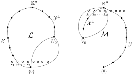
	$\displaystyle U_{0}$	$\displaystyle:=$	$\displaystyle\{x\in{\mathbb{K}}^{n}\mid A_{i}(x,y)=0\ (y\in{\mathbb{K}}^{n})\}.$
	$\displaystyle V_{0}$	$\displaystyle:=$	$\displaystyle\{y\in{\mathbb{K}}^{n}\mid A_{i}(x,y)=0\ (x\in{\mathbb{K}}^{n})\}.$

Let $k:=\mathop{\rm rank}A_{i}$ . An orthogonal frame ${\cal F}=\langle e_{1},e_{2},\ldots,e_{n},f_{1},f_{2},\ldots,f_{n}\rangle$ is a frame of ${\cal L}\times{\cal M}$ satisfying the following conditions:

•

$\langle e_{1},e_{2},\ldots,e_{n}\rangle$ is a frame of ${\cal L}$ .
•

$\langle f_{1},f_{2},\ldots,f_{n}\rangle$ is a frame of ${\cal M}$ .
•

$e_{k+1}\vee e_{k+2}\vee\cdots\vee e_{n}=U_{0}$ .
•

$f_{1}\vee f_{2}\vee\cdots\vee f_{k}=V_{0}$ ( $\Leftrightarrow$ $f_{1}\cap f_{2}\cap\cdots\cap f_{k}=V_{0}$ ).
•

$f_{i}={e_{i}}^{\bot}$ for $i=1,2,\ldots,k$ .

Figure 2 is an intuitive illustration of an orthogonal frame.

Proposition 3.6.

Let ${\cal F}=\langle e_{1},e_{2},\ldots,e_{n},f_{1},f_{2},\ldots,f_{n}\rangle$ be an orthogonal frame. The restriction of the Lovász extension $\overline{R}$ to $K({\cal F})\simeq[0,1]^{n}\times[0,1]^{n}$ can be written as

\overline{R}(x,y)=\sum_{i=1}^{k}\max\{0,x_{i}-y_{i}\},

(3.2)

where $(x_{1},x_{2},\ldots,x_{n})$ is the $\langle e_{1},e_{2},\ldots,e_{n}\rangle$ -coordinate of $x$ and $(y_{1},y_{2},\ldots,y_{n})$ is the $\langle f_{1},f_{2},\ldots,f_{n}\rangle$ -coordinate of $y$ .

Proposition 3.7.

Let ${\cal X}$ and ${\cal Y}$ be maximal chains of ${\cal L}$ and ${\cal M}$ , respectively. Then there exists an orthogonal frame ${\cal F}=\langle e_{1},e_{2},\ldots,e_{n},f_{1},f_{2},\ldots,f_{n}\rangle$ satisfying

{\cal X}\cup{\cal Y}^{\bot}\subseteq\langle e_{1},e_{2},\ldots,e_{n}\rangle,\ {\cal X}^{\bot}\cup{\cal Y}\subseteq\langle f_{1},f_{2},\ldots,f_{n}\rangle.

(3.3)

Such a frame can be found in polynomial time.

Proposition 3.8.

Let ${\cal X}$ and ${\cal Y}$ be maximal chains corresponding to maximal simplices containing $x^{0}$ and $y^{0}$ , respectively. For an orthogonal frame ${\cal F}$ satisfying $(\ref{eqn:XuYbot})$ , the minimizer $(x^{*},y^{*})$ of P2 exists in $K({\cal F})$ .

The above three propositions are proved in Section 3.2.3. Assuming these, we proceed the computation of the resolvent. For an orthogonal frame satisfying (3.3), the problem P2 is equivalent to

	$\displaystyle{\rm P2^{\prime}:\quad Min.}$		$\displaystyle\sum_{i=1}^{k}\max\{0,x_{i}-y_{i}\}+\frac{1}{2\lambda}\left\{\sum_{i=1}^{m}(x_{i}-x^{0}_{i})^{2}+\sum_{i=1}^{n}(y_{i}-y^{0}_{i})^{2}\right\}$
	$\displaystyle{\rm s.t.}$		$\displaystyle 0\leq x_{i}\leq 1,0\leq y_{i}\leq 1\quad(0\leq i\leq n).$

Again this problem is easily solved coordinate-wise. Obviously $x^{*}_{i}=x^{0}_{i}$ and $y^{*}_{i}=y^{0}_{i}$ for $i>k$ . For $i\leq k$ , $(x^{*}_{i},y^{*}_{i})$ is the minimizer of the $2$ -dimensional problem. Obviously this can be solved in constant time.

Theorem 3.9.

The resolvent of $f_{i}=(2n+1)\overline{R_{i}}$ is computed in polynomial time.

Remark 3.10 (Bit complexity).

In the above SPPA, the required bit-length for coefficients of $z\in K({\cal L}\times{\cal M})$ is bounded polynomially in $n,m$ . Indeed, the transformation between the original coordinate and an ${\cal F}$ -coordinate corresponds to multiplying a triangular matrix consisting of $0,\pm 1$ entries; see (2.7). In each iteration $k$ , the optimal solution of quadratic problem P1^′ or P2^′ is obtained by adding (fixed) rational functions in $n,m,k$ to (current points) $x_{i}^{0},y_{i}^{0}$ and multiplying a (fixed) $2\times 2$ rational matrix in $n,m,k$ . Consequently, the bit increase is polynomially bounded.

On the other hand, in the case of ${\mathbb{K}}={\mathbb{Q}}$ , we could not exclude the possibility of an exponential increase of the bit-length for the basis of a vector subspace appearing in the algorithm.

3.2.3 Proofs of Propositions 3.6, 3.7, and 3.8

We start with basic properties of $(\cdot)^{\bot}$ , which follow from elementary linear algebra.

Lemma 3.11.

(1)

If $X\subseteq X^{\prime}$ , then $X^{\bot}\supseteq{X^{\prime}}^{\bot}$ and $\dim{X}^{\bot}-\dim{X^{\prime}}^{\bot}\leq\dim X^{\prime}-\dim X$ .
(2)

$(X+X^{\prime})^{\bot}=X^{\bot}\cap{X^{\prime}}^{\bot}$ .
(3)

$X^{\bot\bot}\supseteq X$ .
(4)

$X\mapsto X^{\bot}$ induces an isomorphism between $[U_{0},{\mathbb{K}}^{n}]$ and $[{\mathbb{K}}^{n},V_{0}]$ with inverse $Y\mapsto Y^{\bot}$ . In particular, $X^{\bot\bot\bot}=X^{\bot}$ .

An alternative expression of $R$ by using $(\cdot)^{\bot}$ is given.

Lemma 3.12.

$R(X,Y)=\dim Y-\dim Y\cap X^{\bot}=\dim X-\dim X\cap Y^{\bot}$ .

Proof.

Consider bases $\{a_{1},a_{2},\ldots,a_{\ell}\}$ of $X$ and $\{b_{1},b_{2},\ldots,b_{\ell^{\prime}}\}$ of $Y$ . We can assume that $\{a_{k^{\prime}+1},a_{k^{\prime}+2},\ldots,a_{\ell^{\prime}}\}$ is a base of $Y\cap X^{\bot}$ . Consider the matrix representation $(A_{i}(a_{i^{\prime}},b_{j^{\prime}}))$ of $A_{i}|_{X\times Y}$ with respect to these bases. Its submatrix of $k^{\prime}+1,k^{\prime}+2,\ldots,\ell^{\prime}$ -th columns is a zero matrix. On the other hand, the submatrix of $1,2,\ldots,k^{\prime}$ -th columns must have the column-full rank $k^{\prime}$ . Thus, the rank $R(X,Y)$ of $A_{i}|_{X\times Y}$ is $k^{\prime}=\ell^{\prime}-(\ell^{\prime}-k^{\prime})=r(Y)-r(Y\cap X^{\bot})$ . The second expression is obtained similarly. ∎

Proof of Proposition 3.6.

An orthogonal frame $\langle e_{1},e_{2},\ldots,e_{n},f_{1},f_{2},\ldots,f_{n}\rangle$ is naturally identified with Boolean lattice $2^{[2n]}\simeq 2^{[n]}\times 2^{[n]}$ . Notice that ${e_{i}}^{\bot}=f_{i}$ if $i\leq k$ and ${e_{i}}^{\bot}={\mathbb{K}}^{n}$ if $i>k$ . The latter fact follows from $e_{i}\subseteq U_{0}\Rightarrow{e_{i}}^{\bot}\supseteq U_{0}^{\bot}={\mathbb{K}}^{n}$ . By Lemma 3.11 (2), we have $X^{\bot}=X\cap\{1,2,\ldots,k\}$ for $X\in 2^{[n]}$ . By Lemma 3.12 and $\dim Y=n-|Y|$ for $Y\in 2^{[n]}\simeq\langle f_{1},f_{2},\ldots,f_{n}\rangle$ (with inclusion order reversed), we have

R(X,Y)=|Y\cup(X\cap[k])|-|Y|=|(X\setminus Y)\cap[k]|.

Identify $2^{[n]}\times 2^{[n]}$ with $\{0,1\}^{n}\times\{0,1\}^{n}$ by $(X,Y)\mapsto(1_{X},1_{Y})$ . Then $R$ is also written as

R(x,y)=\sum_{i=1}^{k}\max\{0,x_{i}-y_{i}\}\quad((x,y)\in\{0,1\}^{n}\times\{0,1\}^{n}).

Observe that the Lovász extension of $(x_{i},y_{i})\mapsto\max\{0,x_{i}-y_{i}\}$ is obtained simply by extending the domain to $[0,1]^{2}$ . Hence, we obtain the desired expression.

Proof of Proposition 3.7.

By Lemma 2.4, we can find (in polynomial time) a frame $\langle e_{1},e_{2},\ldots,e_{n}\rangle$ containing two chains ${\cal X}$ and ${\cal Y}^{\bot}$ . Suppose that ${\cal X}=\{X_{i}\}_{i=0}^{n}$ and ${\cal Y}=\{Y_{i}\}_{i=0}^{n}$ . We can assume that $e_{k+1}\vee e_{k+2}\vee\cdots\vee e_{n}={Y_{0}}^{\bot}=U_{0}$ . Let $f_{i}:={e_{i}}^{\bot}$ for $i=1,2,\ldots,k$ . Then $f_{1}\vee f_{2}\vee\cdots\vee f_{n}=V_{0}$ holds, since, by Lemma 3.11 (2), we have $V_{0}=(e_{1}\vee e_{2}\vee\cdots\vee e_{n})^{\bot}={e_{1}}^{\bot}\vee{e_{2}}^{\bot}\vee\cdots\vee{e_{n}}^{\bot}=f_{1}\vee f_{2}\vee\cdots f_{k}\vee{\mathbb{K}}^{n}\vee\cdots\vee{\mathbb{K}}^{n}=f_{1}\vee f_{2}\vee\cdots\vee f_{k}$ .

Consider the chain ${\cal Y}^{\bot\bot}$ in ${\cal M}$ . Then ${\cal Y}^{\bot\bot}\subseteq\langle f_{1},f_{2},\ldots,f_{k}\rangle$ since each $Y_{i}^{\bot}$ is the join of a subset of $e_{1},e_{2},\ldots,e_{n}$ . Taking $(\cdot)^{\bot}$ as above, $Y_{i}^{\bot\bot}$ is represented as the join of a subset of $f_{1},f_{2},\ldots,f_{k}$ . Consider a consecutive pair $Y_{i-1},Y_{i}$ in ${\cal Y}$ . Consider ${Y_{i-1}}^{\bot\bot}$ and ${Y_{i}}^{\bot\bot}$ . Then, by Lemma 3.11 (3), ${Y_{i-1}}^{\bot\bot}\preceq Y_{i-1}$ and ${Y_{i}}^{\bot\bot}\preceq Y_{i}$ . Suppose that ${Y_{i-1}}^{\bot\bot}\neq{Y_{i}}^{\bot\bot}$ . Then ${Y_{i-1}}^{\bot\bot}\prec:{Y_{i}}^{\bot\bot}$ (by (2.2) and Lemma 3.11 (1)). Thus, for some $f_{j}$ $(1\leq j\leq k)$ , it holds ${Y_{i}}^{\bot\bot}=f_{j}\vee{Y_{i-1}}^{\bot\bot}$ . Here $f_{j}\not\preceq Y_{i-1}$ must hold. Otherwise ${Y_{i-1}}^{\bot\bot}\succeq{f_{j}}^{\bot\bot}={e_{j}}^{\bot\bot\bot}=f_{j}$ , which contradicts ${Y_{i-1}}^{\bot\bot}\prec:{Y_{i}}^{\bot\bot}=f_{j}\vee{Y_{i-1}}^{\bot\bot}$ . Also, $f_{j}\preceq Y_{i}^{\bot\bot}\preceq Y_{i}$ . Thus $Y_{i}=Y_{i-1}\vee f_{j}$ . Therefore, for each $i$ with ${Y_{i-1}}^{\bot\bot}={Y_{i}}^{\bot\bot}$ , we can choose an atom $f$ with $Y_{i}=f\vee Y_{i-1}$ to add to $f_{1},f_{2},\ldots,f_{k}$ , and obtain a required frame $\langle f_{1},f_{2},\ldots f_{n}\rangle$ (containing ${\cal X}^{\bot}$ and ${\cal Y}$ ).

Proof of Proposition 3.8.

Consider retractions $\varphi:=\varphi_{e_{n},e_{n-1},\ldots,e_{k+1},e_{1},e_{2},\ldots,e_{k}}:{\cal L}\to\langle e_{1},e_{2},\ldots,e_{n}\rangle$ and $\phi:=\varphi_{f_{1},f_{2},\ldots,f_{n}}:{\cal M}\to\langle f_{1},f_{2},\ldots,f_{n}\rangle$ ; see Lemma 2.4 (2) for definition. Define a retraction $(\bar{\varphi},\bar{\phi}):K({\cal L})\times K({\cal M})\to K(\langle e_{1},\ldots,e_{n},f_{1},\ldots,f_{n}\rangle)$ by

(\bar{\varphi},\bar{\phi})(x,y):=(\bar{\varphi}(x),\bar{\phi}(y))\quad((x,y)\in K({\cal L})\times K({\cal M}))

Our goal is to show that $(\bar{\varphi},\bar{\phi})$ does not increase the objective value of P2.

First we show

(\phi(Y))^{\bot}=\varphi(Y^{\bot})\quad(Y\in{\cal M}).

(3.4)

Indeed, letting $F_{i}:=f_{1}\vee f_{2}\vee\cdots\vee f_{i}$ and $E_{i}:=e_{1}\vee e_{2}\vee\cdots\vee e_{i}$ , we have

$\displaystyle(\phi(Y))^{\bot}$	$\displaystyle=$	$\displaystyle\left(\bigvee\{f_{i}\mid i\in[n]:Y\wedge F_{i}:\succ Y\wedge F_{i-1}\}\right)^{\bot}$
	$\displaystyle=$	$\displaystyle\left(V_{0}\wedge\bigvee\{f_{i}\mid i\in[n]:Y\wedge F_{i}:\succ Y\wedge F_{i-1}\}\right)^{\bot}$
	$\displaystyle=$	$\displaystyle\left(\bigvee\{f_{i}\mid i\in[k]:Y\wedge F_{i}:\succ Y\wedge F_{i-1}\}\right)^{\bot}$
	$\displaystyle=$	$\displaystyle\left(\bigvee\{f_{i}\mid i\in[k]:(Y\wedge V_{0})\wedge F_{i}:\succ(Y\wedge V_{0})\wedge F_{i-1}\}\right)^{\bot}$
	$\displaystyle=$	$\displaystyle\bigvee\{U_{0}\vee e_{i}\mid i\in[k]:Y^{\bot}\wedge(U_{0}\vee E_{i}):\succ Y^{\bot}\wedge(U_{0}\vee E_{i-1})\}=\varphi(Y^{\bot}).$

The second equality follows from $(V_{0}+Z)^{\bot}=V_{0}^{\bot}\cap Z^{\bot}={\mathbb{K}}^{n}\cap Z^{\bot}=Z^{\bot}$ . The third from the modularity: Let $A:=\bigvee\{f_{i}\mid i\in[k]:Y\wedge F_{i}:\succ Y\wedge F_{i-1}\}$ and $B:=\bigvee\{f_{i}\mid i\in[n]\setminus[k]:Y\wedge F_{i}:\succ Y\wedge F_{i-1}\}$ . Then $V_{0}\wedge B={\mathbb{K}}^{n}$ and $Y=A\vee B$ . Thus we have $A=(V_{0}\wedge B)\vee A=V_{0}\wedge Y$ . The forth follows from $f_{i}\preceq V_{0}$ for $i\in[k]$ . The fifth follows from Lemma 3.11 (4). Note that by $Y^{\bot}\succeq U_{0}$ each atom $e_{i}$ with $i\geq k+1$ is taken in the join of the definition (2.3) of $\varphi=\varphi_{e_{n},e_{n-1},\ldots,e_{k+1},e_{1},e_{2},\ldots,e_{k}}$ .

Next we show

R(\varphi(X),\phi(Y))\leq R(X,Y)\quad(X\in{\cal L},Y\in{\cal M}).

(3.5)

Indeed, for $r=\dim$ , we have $R(\varphi(X),\phi(Y))=r(\varphi(X))-r(\varphi(X)\wedge\phi(Y)^{\bot})=r(X)-r(\varphi(X)\wedge\varphi(Y^{\bot}))\leq r(X)-r(\varphi(X\wedge Y^{\bot}))=r(X)-r(X\wedge Y^{\bot})=R(X,Y).$ In the second equality, we use (3.4) and rank-preserving property of $\varphi$ . The inequality follows from order-preserving property $\varphi(X)\wedge\varphi(Y^{\bot})\succeq\varphi(X\wedge Y^{\bot})$ .

By (3.5), we have $R(\bar{\varphi}(x),\bar{\phi}(y))\leq R(x,y)$ ; recall the isometry between $K({\cal L}\times{\cal M})$ and $K({\cal L})\times K({\cal M})$ (Section 2.2.2). Since $\bar{\varphi}$ and $\bar{\phi}$ are nonexpansive retractions (Proposition 2.5)), we have $d(x^{0},x)\geq d(\bar{\varphi}(x^{0}),\bar{\varphi}(x))=d(x^{0},\bar{\varphi}(x))$ and $d(y^{0},y)\geq d(\bar{\phi}(y^{0}),\bar{\phi}(y))=d(y^{0},\bar{\phi}(y))$ . Thus, $(\bar{\varphi},\bar{\phi})$ has a desired property to prove the statement.

4 A $p$ -adic approach to nc-rank over ${\mathbb{Q}}$

In this section, we consider nc-rank computation of $A=\sum_{i=1}^{m}A_{i}x_{i}$ , where each $A_{i}$ is a matrix over ${\mathbb{Q}}$ . Specifically, we assume that each $A_{i}$ is an integer matrix. As remarked in Remark 3.10, the algorithm in the previous section has no polynomial guarantee for the length of bits representing bases of vector subspaces. Instead of controlling bit sizes, we consider to reduce nc-rank computation over ${\mathbb{Q}}$ to that over $GF(p)$ (for small $p$ ).

For simplicity, we deal with nc-singularity testing of $A$ . Here $A$ is called nc-singular if $\mathop{\rm nc\mbox{-}rank}A<n$ , and called nc-regular if $\mathop{\rm nc\mbox{-}rank}A=n$ . We utilize a relationship between nc-rank and the ordinary rank (on arbitrary field ${\mathbb{K}}$ ). For a positive integer $d$ , the $d$ -blow up $A^{\{d\}}$ of $A$ is a linear symbolic matrix defined by

A^{\{d\}}:=\sum_{i=1}^{m}A_{i}\otimes X_{i},

where $\otimes$ denotes the Kronecker product and $X_{i}=(x_{i,jk})$ is a $d\times d$ matrix with variable entries $x_{i,jk}$ $(i\in[m],j,k\in[d])$ .

Lemma 4.1 ([28, 33]).

A matrix $A$ of form (1.1) is nc-regular if and only if there is a positive integer $d$ such that $A^{\{d\}}$ is regular.

There is an upper bound of such a $d$ . Derksen and Makam[13] proved a polynomial (linear) bound $d\leq n-1$ by utilizing the regularity lemma $d|\mathop{\rm rank}A^{\{d\}}$ in [29]. Such bounds play an essential role in the validity of the algorithms of [17, 29, 30]. Interestingly, our reduction presented below does not use any bound of $d$ .

Fix an arbitrary prime number $p>1$ . Let $v_{p}:{\mathbb{Q}}\to{\mathbb{Z}}\cup\{\infty\}$ denote the $p$ -adic valuation:

v_{p}(u):=k\ {\rm if}\ u=p^{k}a/b,

where $a,b$ are nonzero integers prime to $p$ , and we let $v_{p}(0):=\infty$ . Every rational $u\in{\mathbb{Q}}$ is uniquely represented as the $p$ -adic expansion

u=\sum_{i=k}^{\infty}a_{i}p^{i},

(4.1)

where $k=v_{p}(u)$ and $a_{i}\in\{0,1,2,\ldots,p-1\}$ . The leading (nonzero) coefficient $a_{k}$ is given as the solution of $a=bx\mod p$ . Then $u-a_{k}p^{k}$ is divided by $p^{k+1}$ . Repeating the same procedure for $u-a_{k}p^{k}$ , we obtain the subsequent coefficients in (4.1).

The $2$ -adic expansion of a nonnegative integer $z$ is the same as the binary expression of $z$ , where $v_{2}(z)$ is equal to the number of consecutive zeros from the first bit. This interpretation holds for an arbitrary prime $p$ . In particular, the $p$ -adic valuation of a nonzero integer is bounded by the bit-length in base $p$ :

v_{p}(z)\leq\log_{p}|z|\quad(z\in{\mathbb{Z}}\setminus\{0\}).

(4.2)

The $p$ -adic valuation $v_{p}$ on ${\mathbb{Q}}$ is extended to ${\mathbb{Q}}(x_{1},x_{2},\ldots,x_{m})$ as follows. For a polynomial $f\in{\mathbb{Q}}[x_{1},x_{2},\ldots,x_{m}]$ , define $v_{p}(f)$ by

v_{p}(f):=\min\{v(a)\mid\mbox{$a$ is the coefficient of a term of $f$}\}.

(4.3)

Accordingly, the valuation of a rational function $f/g$ is defined as $v_{p}(f)-v_{p}(g)$ . This is called the Gauss extension of $v_{p}$ .

Our algorithm for testing nc-singularity is based on the following problem (maximum vanishing submodule problem; MVMP):

	$\displaystyle\mbox{MVMP:}\quad{\rm Max}.$		$\displaystyle-v_{p}\det P-v_{p}\det Q$
	$\displaystyle{\rm s.t.}$		$\displaystyle v_{p}(PAQ)_{ij}\geq 0\quad(i,j\in[n]),$
			$\displaystyle P,Q\in GL_{n}({\mathbb{Q}}).$

This problem is definable for an arbitrary field with a discrete valuation, and the following arguments are applicable for such a field, while [25] introduced MVMP for the rational function field with one valuable.

MVMP is also a discrete convex optimization on a CAT(0) space. Indeed, its domain can be viewed as the vertex set (the set of lattices, certain submodules of ${\mathbb{Q}}^{n}$ ) of the Euclidean building for $GL_{n}({\mathbb{Q}})$ , and the objective function is an L-convex function; see [25, 26]. A Euclidean building is a representative space admitting a CAT(0)-metric.

The optimal value of MVMP is denoted by $v_{p}\mathop{\rm Det}^{\prime}A\in{\mathbb{Z}}\cup\{\infty\}$ , where we let $v_{p}\mathop{\rm Det}^{\prime}A:=\infty$ if MVMP is unbounded. The motivation behind this notation $v_{p}\mathop{\rm Det}^{\prime}A$ is explained in Remark 4.6.

For a feasible solution $(P,Q)$ of MVMP, consider the $p$ -adic expansion of $PA_{i}Q=\sum_{k=0}^{\infty}(PA_{i}Q)^{(k)}p^{k}$ for each $i$ . The leading matrix $(PA_{i}Q)^{(0)}$ consists of values $0,1,\ldots,p-1$ and is considered in $GF(p)$ . Then we can consider the linear symbolic matrix

(PAQ)^{(0)}:=\sum_{i=1}^{m}(PA_{i}Q)^{(0)}x_{i}

over $GF(p)$ .

Lemma 4.2.

For a feasible solution $(P,Q)$ of MVMP, the following hold:

(1)

$-v_{p}\det P-v_{p}\det Q\leq v_{p}\det A$ . In particular, $v_{p}\mathop{\rm Det}^{\prime}A\leq v_{p}\det A$ .
(2)

If $(PAQ)^{(0)}$ is regular, then $v_{p}\det A=-v_{p}\det P-v_{p}\det Q=v_{p}\mathop{\rm Det}^{\prime}A$ .

Proof.

They follow from $0\leq v_{p}\det PAQ=v_{p}\det P+v_{p}\det Q+v_{p}\det A$ . The inequality holds in equality precisely when the leading matrix $(PAQ)^{(0)}$ is regular. ∎

The following algorithm for MVMP is due to [25], which originated from Murota’s combinatorial relaxation algorithm [37] and can be viewed as an descent algorithm on the Euclidean building. For an integer vector $z\in{\mathbb{Z}}$ , let $(p^{z})$ denote the diagonal matrix with diagonals $p^{z_{1}},p^{z_{2}},\ldots,p^{z_{n}}$ in order.

Algorithm: Val-Det
0:: Let $(P,Q):=(I,I)$ .
1:: Solve FR (or MVSP) for $(PAQ)^{(0)}$ , and obtain optimal matrices $S,T\in GL_{n}(GF(p))$ such that $S(PAQ)^{(0)}T$ has an $r\times s$ zero submatrix in its upper-left corner.
2:: If $(PAQ)^{(0)}$ is nc-singular, i.e., $n<r+s$ , then let $(P,Q)\leftarrow((p^{-1_{[r]}})SP,QT(p^{1_{[n]\setminus[s]}}))$ and go to step 1. Otherwise stop.

The initial $(P,Q)$ in step 0 is feasible with objection value $0$ , as each $A_{i}$ is an integer matrix. In step 2, $S,T$ are regarded as matrices in $GL_{n}({\mathbb{Q}})$ with entries in $\{0,1,\ldots,p-1\}$ . Observe that each entry in the $r\times s$ upper-left submatrix of $SPAQT$ is divided by $p$ . Thus, the update in step 2 keeps the feasibility of $(P,Q)$ . Further, it strictly increases the objective value: $-v_{p}\det(p^{-1_{[r]}})SP-v_{p}\det QT(p^{1_{[n]\setminus[s]}})=(r+s-n)-v_{p}\det P-v_{p}\det Q$ . Note that $\det S$ and $\det T$ cannot be divided by $p$ , since $S$ and $T$ are invertible in modulo $p$ . Therefore, nc-regularity of $(PAQ)^{(0)}$ is a necessary condition for optimality of $(P,Q)$ . In fact, it is sufficient.

Proposition 4.3 ([26]).

A feasible solution $(P,Q)$ is optimal if and only if $(PAQ)^{(0)}$ is nc-regular. In this case, it holds $v_{p}\mathop{\rm Det}^{\prime}A=(1/d)v_{p}\det A^{\{d\}}$ for some $d>0$ .

Proof.

As in [26, Lemma 4.2 (1)], one can show $v_{p}\mathop{\rm Det}^{\prime}A=(1/d)v_{p}\mathop{\rm Det}^{\prime}A^{\{d\}}$ for all $d$ . By Lemma 4.2, $v_{p}\mathop{\rm Det}^{\prime}A\leq(1/d)v_{p}\det A^{\{d\}}$ holds for all $d$ .

Suppose that $(PAQ)^{(0)}$ is nc-regular. It suffices to show $v_{p}\mathop{\rm Det}^{\prime}A\geq(1/d)v_{p}\det A^{\{d\}}$ for some $d$ . By Lemma 4.1, for some $d>0$ , $((PAQ)^{(0)})^{\{d\}}=((PAQ)^{\{d\}})^{(0)}=((P\otimes I)A^{\{d\}}(Q\otimes I))^{(0)}$ is regular. Observe that $(P\otimes I,Q\otimes I)$ is feasible to MVMP for $A^{\{d\}}$ . By Lemma 4.2 (2), we have $v_{p}\det A^{\{d\}}=-v_{p}\det P\otimes I-v_{p}\det Q\otimes I=-d(v_{p}\det P+v_{p}\det Q)\leq dv_{p}\mathop{\rm Det}^{\prime}A$ . ∎

From the proof and Lemma 4.1, we have:

Corollary 4.4.

$A$ is nc-regular if and only if $v_{p}\mathop{\rm Det}^{\prime}A<\infty$ .

Therefore, Val-Det does not terminate if $A$ is nc-singular. A stopping criterion guaranteeing nc-singularity of $A$ is obtained as follows:

Proposition 4.5.

Suppose that each $A_{i}$ consists of integer entries whose absolute values are at most $D$ . If $A$ is nc-regular, then $v_{p}\mathop{\rm Det}^{\prime}A=O(n\log_{p}nD)$ . Thus, $\Omega(n\log_{p}nD)$ iterations of Val-Det certify nc-singularity of $A$ .

Proof.

Suppose that $A$ is nc-regular. By Proposition 4.3, $v_{p}\mathop{\rm Det}^{\prime}A=(1/d)v_{p}\det A^{\{d\}}$ for some $d$ . We estimate $v_{p}\det A^{\{d\}}$ . The following argument is a sharpening of the proof of [26, Lemma 4.9]. Rewrite $A^{\{d\}}$ as

A^{\{d\}}=\sum_{i\in[m],j,k\in[d]}A_{i,jk}x_{i,jk},

where $A_{i,jk}$ is an $nd\times nd$ block matrix with block size $n$ such that the $(j,k)$ -th block equals to $A_{i}$ and other blocks are zero. By multilinearity of determinant, we have

\det A^{\{d\}}=\sum_{\alpha_{1},\alpha_{2},\ldots,\alpha_{nd}}\pm\det A[\alpha_{1},\alpha_{2},\ldots,\alpha_{nd}]x_{\alpha_{1}}x_{\alpha_{2}}\cdots x_{\alpha_{nd}},

where $\alpha_{\gamma}$ $(\gamma\in[nd])$ ranges over $\{(i,jk)\}_{i\in[m],j\in[d]}$ if $\gamma$ belongs to the $k$ -th block (i.e., $k=\lceil\gamma/d\rceil)$ and $A[\alpha_{1},\alpha_{2},\ldots,\alpha_{nd}]$ is the $nd\times nd$ matrix with the $\gamma$ -th column chosen from $A_{k,ij}$ with $\alpha_{\gamma}=(k,ij)$ . A monomial in this expression is written as $a_{z}\prod x_{k,ij}^{z_{k,ij}}$ for a nonnegative vector $z=(z_{i,jk})\in{\mathbb{Z}}^{md^{2}}$ with $\sum_{i,j}z_{i,jk}=n$ $(k\in[d])$ . The coefficient $a_{z}$ is given by

a_{z}=\sum_{\alpha_{1},\alpha_{2},\ldots,\alpha_{nd}}\pm\det A[\alpha_{1},\alpha_{2},\ldots,\alpha_{nd}],

where $\alpha_{1},\alpha_{2},\ldots,\alpha_{nd}$ are taken so that $(i,jk)$ appears $z_{i,jk}$ times. The total number of such indices is

\prod_{k=1}^{d}\frac{n!}{\prod_{i,j}z_{i,jk}!}\leq n^{nd}.

From Hadamard’s inequality and the fact that each column of $A[\alpha_{1},\alpha_{2},\ldots,\alpha_{nd}]$ has at most $n$ nonzero entries with absolute values at most $D$ , we have

|a_{z}|\leq n^{nd}(n^{1/2}D)^{nd}\leq n^{3nd/2}D^{nd}.

(4.4)

Therefore, the bit length of $a_{z}$ in base $p$ is bounded by $O(nd\log_{p}nD)$ . By (4.2), we have $v_{p}\det A^{\{d\}}=O(nd\log nD)$ . Thus, $v_{p}\mathop{\rm Det}^{\prime}A=O(n\log_{p}nD)$ . ∎

For $p=2$ , the algorithm Val-Det is executed as follows. Instead of updating $(P,Q)$ , update $A$ as $A\leftarrow(p^{-1_{[r]}})SAT(p^{1_{[n]\setminus[s]}})$ . Then, $A^{(0)}$ is computed as $(A_{i})^{(0)}=A_{i}\mod 2$ . In step 2, $S,T$ are $0,1$ matrices such that all entries of the $r\times s$ corner of each $SA_{i}T$ are divided by $2$ . Hence, the next $A_{i}$ is again an integer matrix. The bit-length bound of each entry in $A_{i}$ increases by $O(\log_{2}n)$ (starting from the initial bound $O(\log_{2}D)$ ). Therefore, until detecting nc-singularity of $A$ , the required bit-length is $O(n\log_{2}n\log_{2}nD)$ .

Remark 4.6 (Valuations on the free skew field).

As shown by Cohn [11, Corollary 4.6], any valuation $v$ on a field ${\mathbb{K}}$ is extended to the free skew field ${\mathbb{K}}(\langle x_{1},\ldots,x_{m}\rangle)$ . Then we can consider the valuation $v\mathop{\rm Det}A$ of the Dieudonne determinant $\mathop{\rm Det}A$ of $A$ . If the extension $v$ is discrete and coincides with the Gauss extension (4.3) on ${\mathbb{K}}\langle x_{1},x_{2},\ldots,x_{m}\rangle$ , then one can show by precisely the same argument in [25] that $v\mathop{\rm Det}A$ is given by MVMP. Such an extension seems always exist; in this case, $v_{p}\mathop{\rm Det}^{\prime}=v_{p}\mathop{\rm Det}$ . We verified the existence of an extension with the latter property (by adapting Cohn’s argument in [11, Section 4]). However we could not prove the discreteness. Note that the arguments in this section is independent of the existence issue.

Acknowledgments

We thank Kazuo Murota, Satoru Iwata, Satoru Fujishige, Yuni Iwamasa for helpful comments, and thank Koyo Hayashi for careful reading. The work was partially supported by JSPS KAKENHI Grant Numbers 25280004, 26330023, 26280004, 17K00029, and JST PRESTO Grant Number JPMJPR192A, Japan.

References

[1] P. Abramenko and K. S. Brown, Buildings—Theory and Applications. Springer, New York, 2008.
[2] Z. Allen-Zhu, A. Garg, Y. Li, R. Oliveira, and A. Wigderson. Operator scaling via geodesically convex optimization, invariant theory and polynomial identity testing. preprint, 2017, the conference version in STOC 2018.
[3] M. Bačák, The proximal point algorithm in metric spaces. Israel Journal of Mathematics 194 (2013), 689–701.
[4] M. Bačák, Computing medians and means in Hadamard spaces. SIAM Journal on Optimization 24 (2014), 1542–1566.
[5] M. Bačák, Convex Analysis and Optimization in Hadamard Spaces. De Gruyter, Berlin, 2014.
[6] L. J. Billera, S. P. Holmes, and K. Vogtmann: Geometry of the space of phylogenetic trees. Advances in Applied Mathematics 27 (2001), 733–767.
[7] T. Brady and J. McCammond, Braids, posets and orthoschemes. Algebraic and Geometric Topology 10 (2010), 2277–2314.
[8] M. R. Bridson and A. Haefliger, Metric Spaces of Non-positive Curvature. Springer-Verlag, Berlin, 1999.
[9] P. Bürgisser, C. Franks, A. Garg, R. Oliveira, M. Walter, and A. Wigderson, Towards a theory of non-commutative optimization: geodesic first and second order methods for moment maps and polytopes. preprint, 2019, the conference version in FOCS 2019.
[10] J. Chalopin, V. Chepoi, H. Hirai, and D. Osajda. Weakly modular graphs and nonpositive curvature. Memoirs of the AMS, to appear.
[11] P. M. Cohn, The construction of valuations of skew fields. Journal of the Indian Mathematical Society 54 (1989) 1–45.
[12] P. M. Cohn, Skew fields. Cambridge University Press, Cambridge, 1995.
[13] H. Derksen and V. Makam, Polynomial degree bounds for matrix semi-invariants. Advances in Mathematics 310 (2017), 44–63.
[14] M. Fortin and C. Reutenauer, Commutative/non-commutative rank of linear matrices and subspaces of matrices of low rank. Séminaire Lotharingien de Combinatoire 52 (2004), B52f.
[15] S. Fujishige, Submodular Functions and Optimization, 2nd Edition. Elsevier, Amsterdam, 2005.
[16] S. Fujishige, T Király, K. Makino, K. Takazawa, and S. Tanigawa, Minimizing Submodular Functions on Diamonds via Generalized Fractional Matroid Matchings. EGRES Technical Report (TR-2014-14), (2014).
[17] A. Garg, L. Gurvits, R. Oliveira, and A. Wigderson, Operator scaling: theory and applications. Foundations of Computational Mathematics (2019).
[18] G. Grätzer, Lattice Theory: Foundation. Birkhäuser, Basel, 2011.
[19] L. Gurvits, Classical complexity and quantum entanglement. Journal of Computer and System Sciences 69 (2004), 448–484.
[20] T. Haettel, D. Kielak, and P. Schwer, The 6-strand braid group is CAT(0). Geometriae Dedicata 182 (2016), 263–286.
[21] M. Hamada and H. Hirai, Maximum vanishing subspace problem, CAT(0)-space relaxation, and block-triangularization of partitioned matrix. preprint, 2017.
[22] K. Hayashi, A polynomial time algorithm to compute geodesics in CAT(0) cubical complexes. Discrete & Computational Geometry, to appear.
[23] H. Hirai, Computing DM-decomposition of a partitioned matrix with rank-1 blocks. Linear Algebra and Its Applications 547 (2018), 105–123.
[24] H. Hirai, L-convexity on graph structures. Journal of the Operations Research Society of Japan 61 (2018), 71–109.
[25] H. Hirai, Computing the degree of determinants via discrete convex optimization on Euclidean buildings. SIAM Journal on Applied Geometry and Algebra 3 (2019), 523–557.
[26] H. Hirai and M. Ikeda, A cost-scaling algorithm for computing the degree of determinants, preprint, 2020.
[27] H. Hirai and Y. Iwamasa, A combinatorial algorithm for computing the rank of a generic partitioned matrix with $2\times 2$ submatrices. preprint, 2020, the conference version in IPCO 2020.
[28] P. Hrubeš and A. Wigderson, Non-commutative arithmetic circuits with division. Theory of Computing 11 (2015), 357–393.
[29] G. Ivanyos, Y. Qiao, and K. V. Subrahmanyam, Non-commutative Edmonds’ problem and matrix semi-invariants. Computational Complexity 26 (2017) 717–763.
[30] G. Ivanyos, Y. Qiao, and K. V. Subrahmanyam, Constructive noncommutative rank computation in deterministic polynomial time over fields of arbitrary characteristics. Computational Complexity 27 (2018), 561–593.
[31] H. Ito, S. Iwata, and K. Murota, Block-triangularizations of partitioned matrices under similarity/equivalence transformations. SIAM Journal on Matrix Analysis and Applications 15 (1994), 1226–1255.
[32] S. Iwata and K. Murota, A minimax theorem and a Dulmage-Mendelsohn type decomposition for a class of generic partitioned matrices. SIAM Journal on Matrix Analysis and Applications 16 (1995), 719–734.
[33] D. S. Kaliuzhnyi-Verbovetskyi and V. Vinnikov, Noncommutative rational functions, their difference-differential calculus and realizations. Multidimensional Systems and Signal Processing 23 (2012), 49–77.
[34] F. Kuivinen, On the complexity of submodular function minimisation on diamonds. Discrete Optimization, 8 (2011), 459–477.
[35] L. Lovász, Submodular functions and convexity. In A. Bachem, M. Grötschel, and B. Korte (eds.): Mathematical Programming—The State of the Art (Springer-Verlag, Berlin, 1983), 235–257.
[36] L. Lovász, Singular spaces of matrices and their application in combinatorics. Boletim da Sociedade Brasileira de Matemática 20 (1989), 87–99.
[37] K. Murota, Matrices and Matroids for Systems Analysis. Springer-Verlag, Berlin, 2000.
[38] K. Murota, Discrete Convex Analysis. SIAM, Philadelphia, 2004.
[39] S. Ohta and M. Pálfia, Discrete-time gradient flows and law of large numbers in Alexandrov spaces. Calculus of Variations and Partial Differential Equations 54 (2015) 1591–1610.
[40] T. Oki, Computing the maximum degree of minors in skew polynomial matrices. preprint, 2019, the conference version in ICALP 2020.
[41] M. Owen, Computing geodesic distances in tree space. SIAM Journal on Discrete Mathematics 25 (2011), 1506–1529.

Computing the nc-rank via discrete convex optimization on CAT(0) spaces

Abstract

1 Introduction

Theorem 1.1 ([17, 30]).

Outline.

Theorem 1.2 ([14]).

Organization.

Original motivation: Block triangularization of a partitioned matrix.

2 Preliminaries

2.1 Convex optimization on CAT(0)-spaces

2.1.1 CAT(0)-spaces

Proposition 2.1 ([8, Proposition 1.4]).

Lemma 2.2.

2.1.2 Proximal point algorithm

Theorem 2.3 ([39]).

2.2 Geometry of modular lattices

2.2.1 Frames—Boolean sublattices in a complemented modular lattice

Lemma 2.4 (see e.g.,[18]).

Proof.

2.2.2 The orthoscheme complex of a modular lattice

Proposition 2.5.

The isometry between K​(ℒ)×K​(ℳ)K({\cal L})\times K({\cal M}) and K​(ℒ×ℳ)K({\cal L}\times{\cal M}).

The ℱ{\cal F}-coordinate of a frame ℱ{\cal F}.

2.2.3 Submodular functions and Lovász extensions

Proposition 2.6.

Proof.

3 Algorithm

3.1 Nc-rank is submodular minimization

Lemma 3.1.

Proposition 3.2.

Proof.

3.2 Splitting proximal point algorithm for nc-rank

Theorem 3.3.

Proof.

3.2.1 Computation of the resolvent for fi=−dim¯+(1/8​n)​d​(𝟎,⋅)2f_{i}=-\overline{\dim}+(1/8n)d(\mathbf{0},\cdot)^{2}

Lemma 3.4.

Proof.

Theorem 3.5.

3.2.2 Computation of the resolvent for fi=(2​n+1)​Ri¯f_{i}=(2n+1)\overline{R_{i}}

Proposition 3.6.

Proposition 3.7.

Proposition 3.8.

Theorem 3.9.

Remark 3.10 (Bit complexity).

3.2.3 Proofs of Propositions 3.6, 3.7, and 3.8

Lemma 3.11.

Lemma 3.12.

Proof.

Proof of Proposition 3.6.

Proof of Proposition 3.7.

Proof of Proposition 3.8.

4 A pp-adic approach to nc-rank over ℚ{\mathbb{Q}}

Lemma 4.1 ([28, 33]).

Lemma 4.2.

Proof.

Proposition 4.3 ([26]).

Proof.

Corollary 4.4.

Proposition 4.5.

Proof.

Remark 4.6 (Valuations on the free skew field).

Acknowledgments

References

The isometry between $K({\cal L})\times K({\cal M})$ and $K({\cal L}\times{\cal M})$ .

The ${\cal F}$ -coordinate of a frame ${\cal F}$ .

3.2.1 Computation of the resolvent for $f_{i}=-\overline{\dim}+(1/8n)d(\mathbf{0},\cdot)^{2}$

3.2.2 Computation of the resolvent for $f_{i}=(2n+1)\overline{R_{i}}$

4 A $p$ -adic approach to nc-rank over ${\mathbb{Q}}$