Concentration and regularization of random graphs
Abstract.
This paper studies how close random graphs are typically to their expectations. We interpret this question through the concentration of the adjacency and Laplacian matrices in the spectral norm. We study inhomogeneous Erdös-Rényi random graphs on vertices, where edges form independently and possibly with different probabilities . Sparse random graphs whose expected degrees are fail to concentrate; the obstruction is caused by vertices with abnormally high and low degrees. We show that concentration can be restored if we regularize the degrees of such vertices, and one can do this in various ways. As an example, let us reweight or remove enough edges to make all degrees bounded above by where . Then we show that the resulting adjacency matrix concentrates with the optimal rate: . Similarly, if we make all degrees bounded below by by adding weight to all edges, then the resulting Laplacian concentrates with the optimal rate: . Our approach is based on Grothendieck-Pietsch factorization, using which we construct a new decomposition of random graphs. We illustrate the concentration results with an application to the community detection problem in the analysis of networks.
1. Introduction
Many classical and modern results in probability theory, starting from the Law of Large Numbers, can be expressed as concentration of random objects about their expectations. The objects studied most are sums of independent random variables, martingales, nice functions on product probability spaces and metric measure spaces. For a panoramic exposition of concentration phenomena in modern probability theory and related fields, the reader is referred to the books [25, 9].
This paper studies concentration properties of random graphs. The first step of such study should be to decide how to interpret the statement that a random graph concentrates near its expectation. To do this, it will be useful to look at the graph through the lens of the matrices classically associated with , namely the adjacency and Laplacian matrices.
Let us first build the theory for the adjacency matrix ; the Laplacian will be discussed in Section 1.5. We may say that concentrates about its expectation if is close to its expectation in some natural matrix norm; we interpret the expectation of as the weighted graph with adjacency matrix . Various matrix norms could be of interest here. In this paper, we study concentration in the spectral norm. This automatically gives us a tight control of all eigenvalues and eigenvectors, according to Weyl’s and Davis-Kahan perturbation inequalities (see [5, Sections III.2 and VII.3]).
Concentration of random graphs interpreted this way, and also of general random matrices, has been studied in several communities, in particular in random matrix theory, combinatorics and network science.
We will study random graphs generated from an inhomogeneous Erdös-Rényi model , where edges are formed independently with given probabilities , see [7]. This is a generalization of the classical Erdös-Rényi model where all edge probabilities equal . Many popular graph models arise as special cases of , such as the stochastic block model, a benchmark model in the analysis of networks [22] discussed in Section 1.7, and random subgraphs of given graphs.
Often, the question of interest is estimating some features of the probability matrix from random graphs drawn from . Concentration of adjacency matrix and Laplacian matrix around their expectations, when it holds, guarantees that such features can be recovered. As an example of this use of our concentration results, we will show that if has a block structure, the blocks can be accurately estimated from a single realization of even when the average vertex degree is bounded.
1.1. Dense graphs concentrate
The cleanest concentration results are available for the classical Erdös-Rényi model in the dense regime. In terms of the expected degree , we have with high probability that
| (1.1) |
see [16, 44, 28]. Since , we see that the typical deviation here behaves like the square root of the magnitude of expectation – just like in many other classical results of probability theory. In other words, dense random graphs concentrate well.
The lower bound on density in (1.1) can be essentially relaxed all the way down to . Thus, with high probability we have
| (1.2) |
This result was proved in [15] based on the method developed by J. Kahn and E. Szemeredi [17]. More generally, (1.2) holds for any inhomogeneous Erdös-Rényi model with maximal expected degree . This generalization can be deduced from a recent result of S. Bandeira and R. van Handel [4, Corollary 3.6], while a weaker bound follows from concentration inequalities for sums of independent random matrices [35]. Alternatively, an argument in [15] can be used to prove (1.2) for a somewhat larger but still useful value
| (1.3) |
see [27, 12]. The same can be obtained by using Seginer’s bound on random matrices [20]. As we will see shortly, our paper provides an alternative and completely different approach to general concentration results like (1.2).
1.2. Sparse graphs do not concentrate
In the sparse regime, where the expected degree is bounded, concentration breaks down. According to [24], a random graph from satisfies with high probability that
| (1.4) |
where denotes the maximal degree of the graph (a random quantity). So in this regime we have , which shows that sparse random graphs do not concentrate.
What exactly makes the norm abnormally large in the sparse regime? The answer is, the vertices with too high degrees. In the dense case where , all vertices typically have approximately the same degrees . This no longer happens in the sparser regime ; the degrees do not cluster tightly about the same value anymore. There are vertices with too high degrees; they are captured by the second inequality in (1.4). Even a single high-degree vertex can blow up the norm of the adjacency matrix. Indeed, since the norm of is bounded below by the Euclidean norm of each of its rows, we have .
1.3. Regularization enforces concentration
If high-degree vertices destroy concentration, can we “tame” these vertices? One proposal would be to remove these vertices from the graph altogether. U. Feige and E. Ofek [15] showed that this works for – the removal of the high degree vertices enforces concentration. Indeed, if we drop all vertices with degrees, say, larger than , the the remaining part of the graph satisfies
| (1.5) |
with high probability, where denotes the adjacency matrix of the new graph. The argument in [15] is based on the method developed by J. Kahn and E. Szemeredi [17]. It extends to the inhomogeneous Erdös-Rényi model with defined in (1.3), see [27, 12]. As we will see, our paper provides an alternative and completely different approach to such results.
Although the removal of high degree vertices solves the concentration problem, such solution is not ideal, since those vertices are in some sense the most important ones. In real-world networks, the vertices with highest degrees are “hubs” that hold the network together. Their removal would cause the network to break down into disconnected components, which leads to a considerable loss of structural information.
Would it be possible to regularize the graph in a more gentle way – instead of removing the high-degree vertices, reduce the weights of their edges just enough to keep the degrees bounded by ? The main result of our paper states that this is true. Let us first state this result informally; Theorem 2.1 provides a more general and formal statement.
Theorem 1.1 (Concentration of regularized adjacency matrices).
Consider a random graph from the inhomogeneous Erdös-Rényi model , and let . For all high degree vertices of the graph (say, those with degrees larger than ), reduce the weights of the edges incident to them in an arbitrary way, but so that all degrees of the new (weighted) graph become bounded by . Then, with high probability, the adjacency matrix of the new graph concentrates:
Moreover, instead of requiring that the degrees become bounded by , we can require that the norms of the rows of the new adjacency matrix become bounded by .
1.4. Examples of graph regularization
The regularization procedure in Theorem 1.1 is very flexible. Depending on how one chooses the weights, one can obtain as partial cases several results we summarized earlier, as well as some new ones.
-
1.
Do not do anything to the graph. In the dense regime where , all degrees are already bounded by with high probability. This means that the original graph satisfies . Thus we recover the result of U. Feige and E. Ofek (1.2), which states that dense random graphs concentrate well.
-
2.
Remove all high degree vertices. If we remove all vertices with degrees larger than , we recover another result of U. Feige and E. Ofek (1.5), which states that the removal of the high degree vertices enforces concentration.
-
3.
Remove just enough edges from high-degree vertices. Instead of removing the high-degree vertices with all of their edges, we can remove just enough edges to make all degrees bounded by . This milder regularization still produces the concentration bound (1.5).
-
4.
Reduce the weight of edges proportionally to the excess of degrees. Instead of removing edges, we can reduce the weight of the existing edges, a procedure which better preserves the structure of the graph. For instance, we can assign weight to the edge between vertices and , choosing where is the degree of vertex . One can check that this makes the norms of all rows of the adjacency matrix bounded by . By Theorem 1.1, such regularization procedure leads to the same concentration bound (1.5).
1.5. Concentration of Laplacian
So far, we have looked at random graphs through the lens of their adjacency matrices. A different matrix that captures the geometry of a graph is the (symmmetric, normalized) Laplacian matrix, defined as
| (1.6) |
Here is the identity matrix and is the diagonal matrix with degrees on the diagonal. The reader is referred to [13] for an introduction to graph Laplacians and their role in spectral graph theory. Here we mention just two basic facts: the spectrum of is a subset of , and the smallest eigenvalue is always zero.
Concentration of Laplacians of random graphs has been studied in [35, 11, 39, 23, 18]. Just like the adjacency matrix, the Laplacian is known to concentrate in the dense regime where , and it fails to concentrate in the sparse regime. However, the obstructions to concentration are opposite. For the adjacency matrices, as we mentioned, the trouble is caused by high-degree vertices. For the Laplacian, the problem lies with low-degree vertices. In particular, for the graph is likely to have isolated vertices; they produce multiple zero eigenvalues of , which are easily seen to destroy the concentration.
In analogy to our discussion of adjacency matrices, we can try to regularize the graph to “tame” the low-degree vertices in various ways, for example remove the low-degree vertices, connect them to some other vertices, artificially increase the degrees in the definition (1.6) of Laplacian, and so on. Here we will focus on the following simple way of regularization proposed in [3] and analyzed in [23, 18]. Choose and add the same number to all entries of the adjacency matrix , thereby replacing it with
in the definition (1.6) of the Laplacian. This regularization raises all degrees to . If we choose , the regularized graph does not have low-degree vertices anymore.
The following consequence of Theorem 1.1 shows that such regularization indeed forces Laplacian to concentrate. Here we state this result informally; Theorem 4.1 provides a more formal statement.
Theorem 1.2 (Concentration of the regularized Laplacian).
Consider a random graph from the inhomogeneous Erdös-Rényi model , and let . Choose a number . Then, with high probability, the regularized Laplacian concentrates:
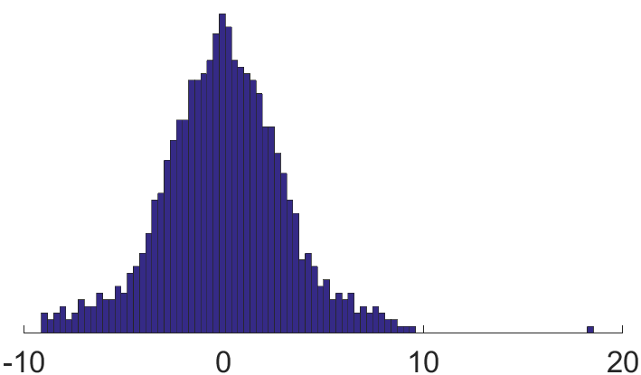
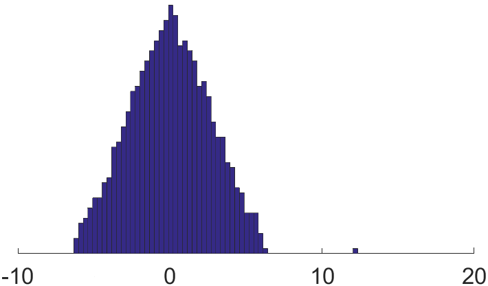
1.6. A numerical experiment
To conclude our discussion of various ways to regularize sparse graphs, let us illustrate the effect of regularization by a numerical experiment. Consider an inhomogeneous Erdös-Rényi graph with vertices, of which have expected degrees and percent have expected degrees . We then regularize the graph by reducing the weights of edges proportionally to the excess of degrees – just as we described in Section 1.4 item 4, except that we use the overall average degree (approximately ) instead of (which results in a more severe weight reduction suitable for our illustration purpose).
Figure 1 shows the histogram of the spectrum of (left) and (right). As we can see, the high degree vertices lead to the long tails in the histogram of the eigenvalues, and regularization shrinks these tails toward the bulk.
1.7. Application: community detection in networks
Concentration of random graphs has an important application to statistical analysis of networks, in particular to the problem of community detection. A common way of modeling communities in networks is the stochastic block model [22], which is a special case of the inhomogeneous Erdös-Rényi model considered in this paper. For the purpose of this example, we focus on the simplest version of the stochastic block model , also known as the balanced planted partition model, defined as follows. The set of vertices is divided into two subsets (communities) of size each. Edges between vertices are drawn independently with probability if they are in the same community and with probability otherwise.
The community detection problem is to recover the community labels of vertices from a single realization of the random graph model. A large literature exists on both the recovery algorithms and the theory establishing when a recovery is possible [14, 33, 34, 32, 1, 29, 8]. There are methods that perform better than a random guess (i.e. the fraction of misclassified vertices is bounded away from as with high probability) under the condition
and no method can perform better than a random guess if this condition is violated.
Moreover, strong consistency, or exact recovery (labeling all vertices correctly with high probability) is possible when the expected degree is of order or larger and and are sufficiently separated, see [32, 30, 6, 20, 10]. Weak consistency (the fraction of mislabeled vertices going to 0 with high probability) is achievable if and only if
see [32]. Many of these results hold in the non-asymptotic regime, for graphs of fixed size . Thus, for any there exists (which only depends on ) such that one can recover communities up to mislabeled vertices as long as
In particular, recovery of communities is possible even for very sparse graphs – those with bounded expected degrees. Several types of algorithms are known to succeed in this regume, including non-backtracking walks [33, 29, 8], spectral methods [12] and methods based on semidefinite programming [19, 31].
As an application of the new concentration results, we show that the regularized spectral clustering [3, 23], one of the simplest most popular algorithms for community detection, can recover communities in the sparse regime. In general, spectral clustering works by computing the leading eigenvectors of either the adjacency matrix or the Laplacian or their regularized versions, and running the -means clustering algorithm on these eigenvectors to recover the node labels. In the simple case of the model , one can simply assign nodes to communities based on the sign (positive or negative) of the corresponding entries of the eigenvector corresponding to the second smallest eigenvalue of regularized Laplacian matrix (or the regularized adjacency matrix ).
Let us briefly explain how our concentration results validate regularized spectral clustering. If the concentration of random graphs holds and is close to , then the standard perturbation theory (Davis-Kahan theorem below) shows that is close to , and in particular, the signs of these two eigenvectors must agree on most vertices. An easy calculation shows that the signs of recover the communities exactly: this vector is a positive constant on one community and a negative constant on the other. Therefore, the signs of must recover the communities up to a small fraction of misclassified vertices.
Before stating our result, let us quote a simple version of the Davis-Kahan theorem perturbation theorem (see e.g. [5, Theorem VII.3.2]).
Theorem 1.3 (Davis-Kahan theorem).
Let be symmetric matrices such that the second smallest eigenvalues of and have multiplicity one and they are of distance at least from the remaining eigenvalues of and . Denote by and the eigenvectors of and corresponding to the second largest eigenvalues of and , respectively. Then
Corollary 1.4 (Community detection in sparse graphs).
Let and . Let be the adjacency matrix drawn from the stochastic block model . Assume that
| (1.7) |
where and is an appropriately large absolute constant. Choose to be the average degree of the graph, i.e. where are vertex degrees. Then with probability at least , we have
In particular, the signs of the entires of correctly estimate the partition into the two communities, up to at most misclassified vertices.
1.8. Organization of the paper
In Section 2, we state a formal version of Theorem 1.1. We show there how to deduce this result from a new decomposition of random graphs, which we state as Theorem 2.6. We prove this decomposition theorem in Section 3. In Section 4, we state and prove a formal version of Theorem 1.2 about the concentration of the Laplacian. We conclude the paper with Section 5 where we propose some questions for further investigation.
Acknowledgement
The authors are grateful to Ramon van Handel for several insightful comments on the preliminary version of this paper.
2. Full version of Theorem 1.1, and reduction to a graph decomposition
In this section we state a more general and quantitative version of Theorem 1.1, and we reduce it to a new form of graph decomposition, which can be of interest on its own.
Theorem 2.1 (Concentration of regularized adjacency matrices).
Consider a random graph from the inhomogeneous Erdös-Rényi model , and let . For any , the following holds with probability at least . Consider any subset consisting of at most vertices, and reduce the weights of the edges incident to those vertices in an arbitrary way. Let be the maximal degree of the resulting graph. Then the adjacency matrix of the new (weighted) graph satisfies
Moreover, the same bound holds for being the maximal norm of the rows of .
In this result and in the rest of the paper, denote absolute constants whose values may be different from line to line.
Remark 2.2 (Theorem 2.1 implies Theorem 1.1).
The subset of vertices in Theorem 2.1 can be completely arbitrary. So let us choose the high-degree vertices, say those with degrees larger than . There are at most such vertices with high probability; this follows by an easy calculation, and also from Lemma 3.5. Thus we immediately deduce Theorem 1.1.
Remark 2.3 (Tight upper bound).
Remark 2.4 (Method to prove Theorem 2.1).
One may wonder if Theorem 2.1 can be proved by developing an -net argument similar to the method of J. Kahn and E. Szemeredi [17] and its versions [2, 15, 27, 12]. Although we can not rule out such possibility, we do not see how this method could handle a general regularization. The reader familiar with the method can easily notice an obstacle. The contribution of the so-called light couples becomes hard to control when one changes, and even reduces, the individual entries of (the weights of edges).
We will develop an alternative and somewhat simpler approach, which will be able to handle a general regularization of random graphs. It sheds light on the specific structure of graphs that enables concentration. We are going to identify this structure through a graph decomposition in the next section. But let us pause briefly to mention the following useful reduction.
Remark 2.5 (Reduction to directed graphs).
Our arguments will be more convenient to carry out if the adjacency matrix has all independent entries. To be able to make this assumption, we can decompose into the upper-triangular and a lower-triangular parts, both of which have independent entries. If we can show that each of these parts concentrate about its expectation, it would follow that concentrate about by triangle inequality.
In other words, we may prove Theorem 2.1 for directed inhomogeneous Erdös-Rényi graphs, where edges between any vertices and in any direction appear indepednently with probabilities . In the rest of the argument, we will only work with such random directed graphs.
2.1. Graph decomposition
In this section, we reduce Theorem 2.1 to the following decomposition of inhomogeneous Erdös-Rényi directed random graphs. This decomposition may have an independent interest. Throughout the paper, we denote by the matrix which coincides with a matrix on a subset of edges and has zero entries elsewhere.
Theorem 2.6 (Graph decomposition).
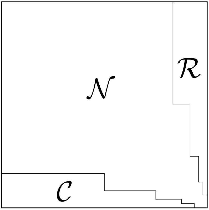
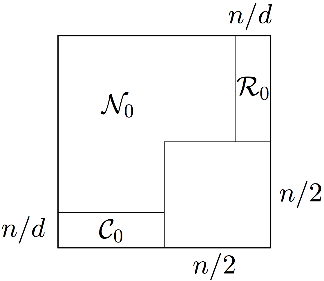
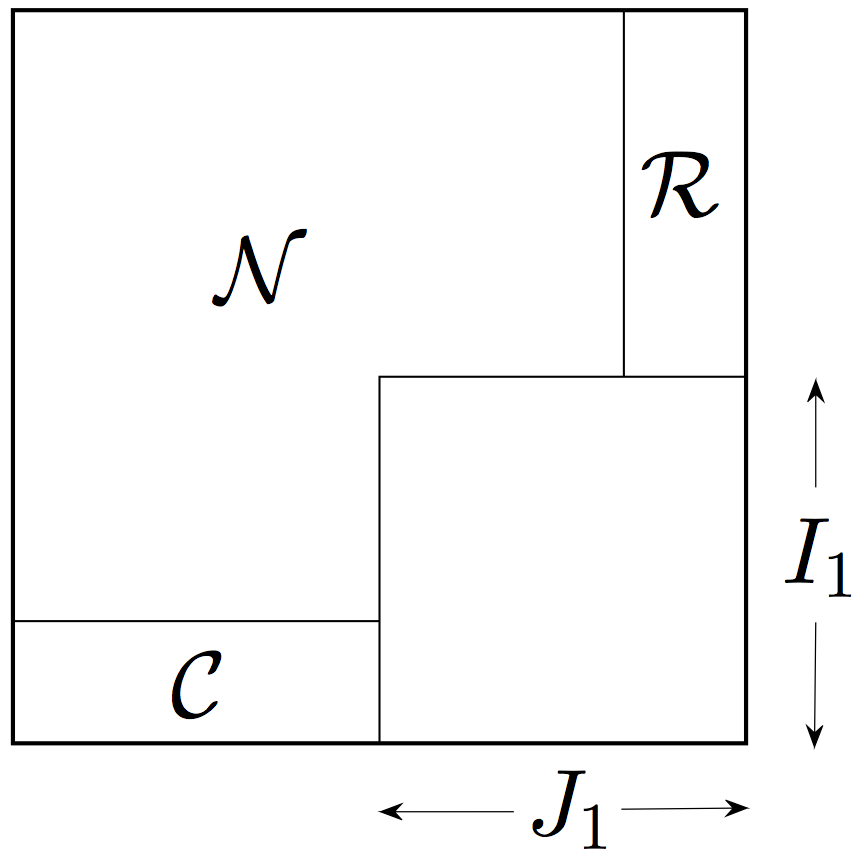
Consider a random directed graph from the inhomogeneous Erdös-Rényi model, and let be as in (1.3). For any , the following holds with probability at least . One can decompose the set of edges into three classes , and so that the following properties are satisfied for the adjacency matrix .
-
•
The graph concentrates on , namely .
-
•
Each row of and each column of has at most ones.
Moreover, intersects at most columns, and intersects at most rows of .
Figure 2 illustrates a possible decomposition Theorem 2.6 can provide. The edges in form a big “core” where the graph concentrates well even without regularization. The edges in and can be thought of (at least heuristically) as those attached to high-degree vertices.
2.2. Deduction of Theorem 2.1
First, let us explain informally how the graph decomposition could lead to Theorem 2.1. The regularization of the graph does not destroy the properties of , and in Theorem 2.6. Moreover, regularization creates a new property for us, allowing for a good control of the columns of and rows of . Let us focus on to be specific. The norms of all columns of this matrix are at most , and the norms of all rows are by Theorem 2.6. By a simple calculation which we will do in Lemma 2.7, this implies that . A similar bound can be proved for . Combining , and together will lead to the error bound in Theorem 2.1.
To make this argument rigorous, let us start with the simple calculation we just mentioned.
Lemma 2.7.
Consider a matrix in which each row has norm at most , and each column has norm at most . Then .
Proof.
Let be a vector with . Using Cauchy-Schwarz inequality and the assumptions, we have
Since is arbitrary, this completes the proof. ∎
Remark 2.8 (Riesz-Thorin interpolation theorem implies Lemma 2.7).
We are ready to formally deduce the main part of Theorem 2.1 from Theorem 2.6; we defer the “moreover” part to Section 3.6.
Proof of Theorem 2.1 (main part)..
Fix a realization of the random graph that satisfies the conclusion of Theorem 2.6, and decompose the deviation as follows:
| (2.1) |
We will bound the spectral norm of each of the three terms separately.
Step 1. Deviation on . Let us further decompose
| (2.2) |
By Theorem 2.6, . To control the second term in (2.2), denote by the subset of edges that are reweighed in the regularization process. Since and are equal on , we have
| (2.3) |
Further, a simple restriction property implies that
| (2.4) |
Indeed, restricting a matrix onto a product subset of can only reduce its norm. Although the set of reweighted edges is not a product subset, it can be decomposed into two product subsets:
| (2.5) |
where is the subset of vertices incident to the edges in . Then (2.4) holds; right hand side of that inequality is bounded by by Theorem 2.6. Thus we handled the first term in (2.3).
To bound the second term in (2.3), we can use another restriction property that states that the norm of the matrix with non-negative entries can only reduce by restricting onto any subset of (whether a product subset or not). This yields
| (2.6) |
where the second inequality follows by (2.5). By assumption, the matrix has rows and each of its entries is bounded by . Hence the norm of all rows is bounded by , and the norm of all columns is bounded by . Lemma 2.7 implies that . A similar bound holds for the second term of (2.6). This yields
so we handled the second term in (2.3). Recalling that the first term there is bounded by , we conclude that .
Returning to (2.2), we recall that the first term in the right hand is bounded by , and we just bounded the second term by . Hence
Step 2. Deviation on and . By triangle inequality, we have
Recall that entrywise. By Theorem 2.6, each of the rows of , and thus also of , has norm at most . Moreover, by definition of , each of the columns of , and thus also of , has norm at most . Lemma 2.7 implies that .
3. Proof of Decomposition Theorem 2.6
3.1. Outline of the argument
We will construct the decomposition in Theorem 2.6 by an iterative procedure. The first and crucial step is to find a big block111In this paper, by block we mean a product set with arbitrary index subsets . These subsets are not required to be intervals of successive integers. of size at least on which concentrates, i.e.
To find such block, we first establish concentration in norm; this can be done by standard probabilistic techniques. Next, we can automatically upgrade this to concentration in the spectral norm () once we pass to an appropriate block . This can be done using a general result from functional analysis, which we call Grothendieck-Pietsch factorization.
Repeating this argument for the transpose, we obtain another block of size at least where the graph concentrates as well. So the graph concentrates on . The “core” will form the first part of the class we are constructing.
It remains to control the graph on the complement of . That set of edges is quite small; it can be described as a union of a block with rows, a block with columns and an exceptional block; see Figure 3(b) for illustration. We may consider and as the first parts of the future classes and we are constructing.
Indeed, since has so few rows, the expected number of ones in each column of is bounded by . For simplicity, let us think that all columns of have ones as desired. (In the formal argument, we will add the bad columns to the exceptional block.) Of course, the block can be handled similarly.
At this point, we decomposed into , , and an exceptional block. Now we repeat the process for the exceptional block, constructing , , and there, and so on. Figure 3(c) illustrates this process. At the end, we choose , and to be the unions of the blocks , and respectively.
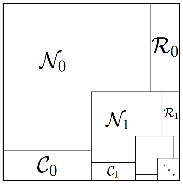
Two precautions have to be taken in this argument. First, we need to make concentration on the core blocks better at each step, so that the sum of those error bounds would not depend of the total number of steps. This can be done with little effort, with the help of the exponential decrease of the size of the blocks . Second, we have a control of the sizes but not locations of the exceptional blocks. Thus to be able to carry out the decomposition argument inside an exceptional block, we need to make the argument valid uniformly over all blocks of that size. This will require us to be delicate with probabilistic arguments, so we can take a union bound over such blocks.
3.2. Grothendieck-Pietsch factorization
As we mentioned in the previous section, our proof of Theorem 2.6 is based on Grothendieck-Pietsch factorization. This general and well known result in functional analysis [36, 37] has already been used in a similar probabilistic context, see [26, Proposition 15.11].
Grothendieck-Pietsch factorization compares two matrix norms, the norm (which we call the spectral norm ) and the norm. For a matrix , these norms are defined as
The norm is usually easier to control, since the supremum is taken with respect to the discrete set , and any vector there has all coordinates of the same magnitude.
To compare the two norms, one can start with the obvious inequality
Both parts of this inequality are optimal, so there is an unavoidable slack between the upper and lower bounds. However, Grothendieck-Pietsch factorization allows us to tighten the inequality by changing sightly. The next two results offer two ways to change – introduce weights and pass to a sub-matrix.
Theorem 3.1 (Grothendieck-Pietsch’s factorization, weighted version).
Let be a real matrix. Then there exist positive weights with such that
| (3.1) |
where denotes the diagonal matrix with weights on the diagonal.
This result is a known combination of the Little Grothendieck Theorem (see [41, Corollary 10.10] and [38]) and Pietsch Factorization (see [41, Theorem 9.2]). In an explicit form, a version of this result can be found e.g. in [26, Proposition 15.11]. The weights can be computed algorithmically, see [42].
The following related version of Grothendieck-Pietsch’s factorization can be especially useful in probabilistic contexts, see [26, Proposition 15.11]. Here and in the rest of the paper, we denote by the sub-matrix of a matrix with rows indexed by a subset and columns indexed by a subset .
Theorem 3.2 (Grothendieck-Pietsch factorization, sub-matrix version).
Let be a real matrix and . Then there exists with such that
Proof.
Consider the weights given by Theorem 3.1, and choose to consist of the indices satisfying . Since , the set must contain at least indices as claimed. Furthermore, the diagonal entries of are all bounded from below by , which yields
On the other hand, by (3.1) the left-hand side of this inequality is bounded by . Rearranging the terms, we complete the proof. ∎
3.3. Concentration on a big block
We are starting to work toward constructing the core part in Theorem 2.6. In this section we will show how to find a big block on which the adjacency matrix concentrates. First we will establish concentration in norm, and then, using Grothendieck-Pietsch factorization, in the spectral norm.
The lemmas of this and next section should be best understood for , and . In this case, we are working with the entire adjacency matrix, and trying to make the first step in the iterative procedure. The further steps will require us to handle smaller blocks ; the parameter will then become smaller in order to achieve better concentration for smaller blocks.
Lemma 3.3 (Concentration in norm).
Let and . Then for the following holds with probability at least . Consider a block of size . Let be the set of indices of the rows of that contain at most ones. Then
| (3.2) |
Proof.
By definition,
| (3.3) |
where we denoted
Let us first fix a block and a vector . Let us analyze the independent random variables . Since , it follows by definition of that
| (3.4) |
A more useful bond will follow from Bernstein’s inequality. Indeed, is a sum of independent random variables with zero means and variances at most . By Bernstein’s inequality, for any we have
| (3.5) |
For , this can be further bounded by , once we use the assumption . For , the left-hand side of (3.5) is automatically zero by (3.4). Therefore
| (3.6) |
We are now ready to bound the right-hand side of (3.3). By (3.6), the random variable is sub-gaussian222For definitions and basic facts about sub-gaussian random variables, see e.g. [43]. with sub-gaussian norm at most . It follows that is sub-exponential with sub-exponential norm at most . Using Bernstein’s inequality for sub-exponential random variables (see Corrollary 5.17 in [43]), we have
| (3.7) |
Choosing , we bound this probability by .
Applying Lemma 3.3 followed by Grothendieck-Piesch factorization (Theorem 3.2), we obtain the following.
Lemma 3.4 (Concentration in spectral norm).
Let and . Then for the following holds with probability at least . Consider a block of size . Let be the set of indices of the rows of that contain at most ones. Then one can find a subset of at least columns such that
| (3.9) |
3.4. Restricted degrees
The two simple lemmas of this section will help us to handle the part of the adjacency matrix outside the core block constructed in Lemma 3.4. First, we show that almost all rows have at most ones, and thus are included in the core block.
Lemma 3.5 (Degrees of subgraphs).
Let and . Then for the following holds with probability at least . Consider a block of size . Then all but rows of have at most ones.
Proof.
Fix a block , and denote by the number of ones in the -th row of . Then by the assumption. Using Chernoff’s inequality, we obtain
Let be the number of rows with . Then is a sum of independent Bernoulli random variables with expectations at most . Again, Chernoff’s inequality implies
The second inequality here holds since . (To see this, notice that the definition of and assumption on imply that .)
It remains to take a union bound over all blocks . We obtain that the conclusion of the lemma holds with probability at least
In the last inequality we used the assumption that . The proof is complete. ∎
Next, we handle the block of rows that do have too many ones. We show that most columns of this block have ones.
Lemma 3.6 (More on degrees of subgraphs).
Let and . Then for the following holds with probability at least . Consider a block of size with some . Then all but columns of have at most ones.
Proof.
Fix and , and denote by the number of ones in the -th column of . Then by assumption. Using Chernoff’s inequality, we have
Let be the number of columns with . Then is a sum of independent Bernoulli random variables with expectations at most . Again, Chernoff’s inequality implies
The second inequality here holds since , which in turn follows by assumption on .
It remains to take a union bound over all blocks . It is enough to consider the blocks with largest possible number of columns, thus with . We obtain that the conclusion of the lemma holds with probability at least
In the last inequality we used the assumption that . The proof is complete. ∎
3.5. Iterative decomposition: proof of Theorem 2.1
Finally, we combine the tools we developed so far, and we construct an iterative decomposition of the adjacency matrix the way we outline in Section 3.1. Let us set up one step of this procedure, where we consider an block and decompose almost all of it (everything except an block) into classes , and satisfying the conclusion of Theorem 2.6. Once we can do this, we repeat the procedure for the block, etc.
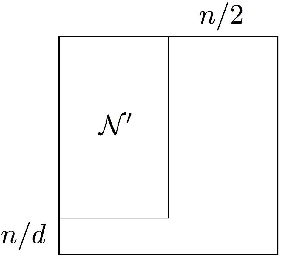
Lemma 3.7 (Decomposition of a block).
Let and . Then for the following holds with probability at least . Consider a block of size . Then there exists an exceptional sub-block with dimensions at most such that the remaining part of the block, that is , can be decomposed into three classes , and so that the following holds.
-
•
The graph concentrates on , namely .
-
•
Each row of and each column of has at most ones.
Moreover, intersects at most columns and intersects at most rows of .
After a permutation of rows and columns, a decomposition of the block stated in Lemma 3.7 can be visualized in Figure 4(c).
Proof.
Since we are going to use Lemmas 3.4, 3.5 and 3.6, let us fix realization of the random graph that satisfies the conclusion of those three lemmas.
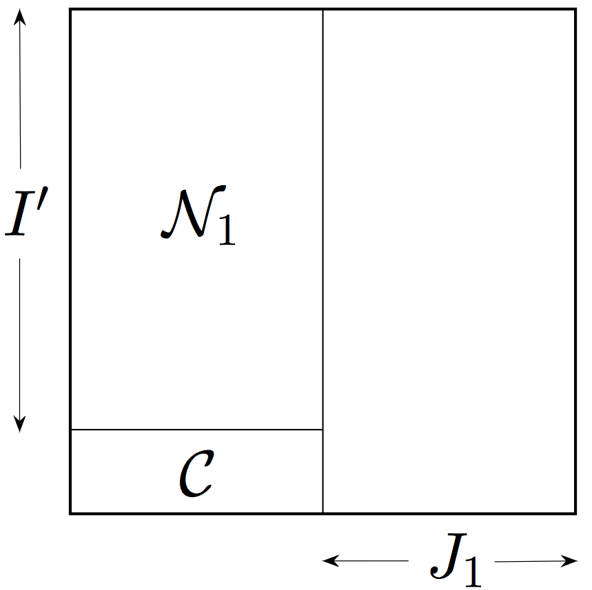
By Lemma 3.5, all but rows of have at most ones; let us denote by the set of indices of those rows with at most ones. Then we can use Lemma 3.4 for the block and with replaced by ; the choice of ensures that all rows have small numbers of ones, as required in that lemma. To control the rows outside , we may use Lemma 3.6 for ; as we already noted, this block has at most rows as required in that lemma. Intersecting the good sets of columns produced by those two lemmas, we obtain a set of at most exceptional columns such that the following holds.
-
•
On the block , we have
-
•
For the block , all columns of have at most ones.
Figure 4(a) illustrates the decomposition of the block into the set of exceptional columns indexed by and good sets and .
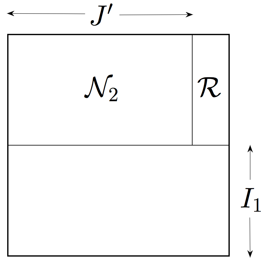
To finish the proof, we apply the above argument to the transpose on the block . To be precise, we start with the set of all but small columns of (those with at most ones); then we obtain an exceptional set of at most rows; and finally we conclude that concentrates on the block and has small rows on the block . Figure 4(b) illustrates this decomposition.
It only remains to combine the decompositions for and ; Figure 4(c) illustrates a result of the combination. Once we define , it becomes clear that , and have the required properties.333It may happen that an entry ends up in more than one class , and . In such cases, we split the tie arbitrarily. ∎
Proof of Theorem 2.6.
Let us fix a realization of the random graph that satisfies the conclusion of Lemma 3.7. Applying that lemma for and with , we decompose the set of edges into three classes , and plus an exceptional block . Apply Lemma 3.7 again, this time for the block , for and with . We decompose into , and plus an exceptional block .
Repeat this process for where is the running size of the block; we halve this size at each step, and so we have . Figure 3(c) illustrates a decomposition that we may obtain this way. In a finite number of steps (actually, in steps) the exceptional block becomes empty, and the process terminates. At that point we have decomposed the set of edges into , and , defined as the union of , and respectively, which we obtained at each step. It is clear that and satisfy the required properties.
It remains to bound the deviation of on . By construction, satisfies
Thus, by triangle inequality we have
In the second inequality we used that , which forces the series to converge. The proof of Theorem 2.6 is complete. ∎
3.6. Replacing the degrees by the norms in Theorem 2.1
Let us now prove the “moreover” part of Theorem 2.1, where is the the maximal norm of the rows and columns of the regularized adjacency matrix . This is clearly a stronger statement than in the main part of the theorem. Indeed, since all entries of are bounded in absolute value by , each degree, being the norm of a row, is bounded below by the norm squared.
This strengthening is in fact easy to check. To do so, note that the definition of was used only once in the proof of Theorem 2.1, namely in Step 2 where we bounded the norms of and . Thus, to obtain the strengthening, it is enough to replace the application of Lemma 2.7 there by the following lemma.
Lemma 3.8.
Consider a matrix with entries in . Suppose each row of has at most non-zero entries, and each column has norm at most . Then .
Proof.
To prove the claim, let be a vector with . Using Cauchy-Schwarz inequality and the assumptions, we have
Since is arbitrary, this completes the proof. ∎
4. Concentration of the regularized Laplacian
In this section, we state the following formal version of Theorem 1.2, and we deduce it from concentration of adjacency matrices (Theorem 2.1).
Theorem 4.1 (Concentration of regularized Laplacians).
Consider a random graph from the inhomogeneous Erdös-Rényi model, and let be as in (1.3). Choose a number . Then, for any , with probability at least one has
Proof.
Two sources contribute to the deviation of Laplacian – the deviation of the adjacency matrix and the deviation of the degrees. Let us separate and bound them individually.
Step 1. Decomposing the deviation. Let us denote for simplicity; then
Here and are the diagonal matrices with degrees of and on the diagonal, respectively. Using the fact that , we can represent the deviation as
Let us bound and separately.
Step 2. Bounding . Let us introduce a diagonal matrix that should be easier to work with than . Set if and otherwise. Then entries of are upper bounded by the corresponding entries of , and so
Next, by triangle inequality,
| (4.1) |
In order to bound , we use Theorem 2.1 to show that concentrates around . This should be possible because is obtained from by reducing the degrees that are bigger than . To apply the “moreover” part of Theorem 2.1, let us check the magnitude of the norms of the rows of :
Here in the first inequality we used that and ; the second inequality follows by definition of . Applying Theorem 2.1, we obtain with probability that
To bound , we note that by construction of , the matrices and coincide on the block , where is the set of vertices satisfying . This block is very large – indeed, Lemma 3.5 implies that with probability . Outside this block, i.e. on the small blocks and , the entries of are bounded by the corresponding entries of , which are all bounded by . Thus, using Lemma 2.7, we have
Substituting the bounds for and into (4.1), we conclude that
with probability at least .
Step 3. Bounding . Bounding the spectral norm by the Hilbert-Schmidt norm, we get
and and . To bound , we note that
Recalling the definition of and and adding and subtracting , we have
So, using the inequality and bounding by , we obtain
| (4.2) |
We claim that
| (4.3) |
Indeed, since the variance of each is bounded by , the expectation of the sum in (4.3) is bounded by . To upgrade the variance bound to an exponential deviation bound, one can use one of the several standard methods. For example, Bernstein’s inequality implies that satisfies for all . This means that the random variable belongs to the Orlicz space and has norm , see [26]. By triangle inequality, we conclude that , which in turn implies (4.3).
5. Further questions
5.1. Optimal regularization?
The main point of our paper was that regularization helps sparse graphs to concentrate. We have discussed several kinds of regularization in Section 1.4 and mentioned some more in Section 1.4. We found that any meaningful regularization works, as long as it reduces the too high degrees and increases the too low degrees. Is there an optimal way to regularize a graph? Designing the best “preprocessing” of sparse graphs for spectral algorithms is especially interesting from the applied perspective, i.e. for real world networks.
On the theoretical level, can regularization of sparse graphs produce the same optimal bound that we saw for dense graphs in (1.1)? Thus, an ideal regularization should bring all parasitic outliers of the spectrum into the bulk. If so, this would lead to a potentially simple spectral clustering algorithm for community detection in networks which matches the theoretical lower bounds. Algorithms with optimal rates exist for this problem [33, 29], but their analysis is very technical.
5.2. How exactly concentration depends on regularization?
It would be interesting to determine how exactly the concentration of Laplacian depends on the regularization parameter . The dependence in Theorem 4.1 is not optimal, and we have not made efforts to improve it. Although it is natural to choose as in Theorem 1.2, choosing could also be useful [23]. Choosing may be interesting as well, for then and we obtain the concentration of around the Laplacian of the expectation of the original (rather than regularized) matrix .
5.3. Average expected degree?
5.4. From random graphs to random matrices?
Adjacency matrices of random graphs are particular examples of random matrices. Does the phenomenon we described, namely that regularization leads to concentration, apply for general random matrices? Guided by Theorem 1.1, we might expect the following for a broader general class of random matrices with mean zero independent entries. First, the only reason the spectral norm of is too large (and that it is determined by outliers of spectrum) could be the existence of a large row or column. Furthermore, it might be possible to reduce the norm of (and thus bring the outliers into the bulk of spectrum) by regularizing in some way the rows and columns that are too large. For related questions in random matrix theory, see the recent work [4, 21].
References
- [1] E. Abbe, A. S. Bandeira, and G. Hall. Exact recovery in the stochastic block model. IEEE Transactions on Information Theory, 62(1):471–487, 2016.
- [2] N. Alon and N. Kahale. A spectral technique for coloring random 3-colorable graphs. SIAM J. Comput., (26):1733–1748, 1997.
- [3] A. A. Amini, A. Chen, P. J. Bickel, and E. Levina. Pseudo-likelihood methods for community detection in large sparse networks. The Annals of Statistics, 41(4):2097–2122, 2013.
- [4] A. Bandeira and R. V. Handel. Sharp nonasymptotic bounds on the norm of random matrices with independent entries. Annals of Probability, to appear, 2014.
- [5] R. Bhatia. Matrix Analysis. Springer-Verlag New York, 1996.
- [6] P. J. Bickel and A. Chen. A nonparametric view of network models and Newman-Girvan and other modularities. Proc. Natl. Acad. Sci. USA, 106:21068–21073, 2009.
- [7] B. Bollobas, S. Janson, and O. Riordan. The phase transition in inhomogeneous random graphs. Random Structures and Algorithms, 31:3–122, 2007.
- [8] C. Bordenave, M. Lelarge, and L. Massoulié. Non-backtracking spectrum of random graphs: community detection and non-regular Ramanujan graphs. arxiv:1501.06087, 2015.
- [9] S. Boucheron, G. Lugosi, and P. Massart. Concentration inequalities: a nonasymptotic theory of independence. Oxford University Press, 2013.
- [10] T. Cai and X. Li. Robust and computationally feasible community detection in the presence of arbitrary outlier nodes. Ann. Statist., 43(3):1027–1059, 2015.
- [11] K. Chaudhuri, F. Chung, and A. Tsiatas. Spectral clustering of graphs with general degrees in the extended planted partition model. Journal of Machine Learning Research Workshop and Conference Proceedings, 23:35.1 – 35.23, 2012.
- [12] P. Chin, A. Rao, and V. Vu. Stochastic block model and community detection in the sparse graphs : A spectral algorithm with optimal rate of recovery. arXiv:1501.05021, 2015.
- [13] F. R. K. Chung. Spectral Graph Theory. CBMS Regional Conference Series in Mathematics, 1997.
- [14] A. Decelle, F. Krzakala, C. Moore, and L. Zdeborová. Asymptotic analysis of the stochastic block model for modular networks and its algorithmic applications. Physical Review E, 84:066106, 2011.
- [15] U. Feige and . Ofek. Spectral techniques applied to sparse random graphs. Wiley InterScience, 2005.
- [16] Z. Füredi and J. Komlós. The eigenvalues of random symmetric matrices. Combinatorica, 1:3:233–241, 1980.
- [17] J. Friedman, J. Kahn, and E. Szemeredi. On the second eigenvalue in random regular graphs. Proc Twenty First Annu ACMSymp Theory of Computing, pages 587–598, 1989.
- [18] C. Gao, Z. Ma, A. Y. Zhang, and H. H. Zhou. Achieving optimal misclassification proportion in stochastic block model. arXiv:1505.03772, 2015.
- [19] O. Guédon and R. Vershynin. Community detection in sparse networks via grothendieck’s inequality. Probability Theory and Related Fields, to appear, 2014.
- [20] B. Hajek, Y. Wu, and J. Xu. Achieving exact cluster recovery threshold via semidefinite programming. arXiv:1412.6156, 2014.
- [21] R. V. Handel. On the spectral norm of inhomogeneous random matrices. arXiv:1502.05003, 2015.
- [22] P. W. Holland, K. B. Laskey, and S. Leinhardt. Stochastic blockmodels: first steps. Social Networks, 5(2):109–137, 1983.
- [23] A. Joseph and B. Yu. Impact of regularization on spectral clustering. Ann. Statist., 44(4):1765–1791, 2016.
- [24] M. Krivelevich and B. Sudakov. The largest eigenvalue of sparse random graphs. Combin Probab Comput, 12:61–72, 2003.
- [25] M. Ledoux. The Concentration of Measure Phenomenon, volume 89 of Mathematical Surveys and Monographs. Amer. Math. Society, 2001.
- [26] M. Ledoux and M. Talagrand. Probability in Banach spaces: Isoperimetry and processes. Springer-Verlag, Berlin, 1991.
- [27] J. Lei and A. Rinaldo. Consistency of spectral clustering in stochastic block models. Ann. Statist., 43(1):215–237, 2015.
- [28] L. Lu and X. Peng. Spectra of edge-independent random graphs. The electronic journal of combinatorics, 20(4), 2013.
- [29] L. Massoulié. Community detection thresholds and the weak Ramanujan property. In Proceedings of the 46th Annual ACM Symposium on Theory of Computing, STOC ’14, pages 694–703, 2014.
- [30] McSherry. Spectral partitioning of random graphs. Proc. 42nd FOCS, pages 529–537, 2001.
- [31] A. Montanari and S. Sen. Semidefinite programs on sparse random graphs and their application to community detection. arXiv:1504.05910, 2015.
- [32] E. Mossel, J. Neeman, and A. Sly. Consistency thresholds for binary symmetric block models. arXiv:1407.1591, 2014.
- [33] E. Mossel, J. Neeman, and A. Sly. A proof of the block model threshold conjecture. arXiv:1311.4115, 2014.
- [34] E. Mossel, J. Neeman, and A. Sly. Reconstruction and estimation in the planted partition model. Probability Theory and Related Fields, 2014.
- [35] R. Oliveira. Concentration of the adjacency matrix and of the laplacian in random graphs with independent edges. arXiv:0911.0600, 2010.
- [36] A. Pietsch. Operator Ideals. North-Holland Amsterdam, 1978.
- [37] G. Pisier. Factorization of linear operators and geometry of Banach spaces. Number 60 in CBMS Regional Conference Series in Mathematics. AMS, Providence, 1986.
- [38] G. Pisier. Grothendieck’s theorem, past and present. Bulletin (New Series) of the American Mathematical Society, 49(2):237–323, 2012.
- [39] T. Qin and K. Rohe. Regularized spectral clustering under the degree-corrected stochastic blockmodel. In Advances in Neural Information Processing Systems, pages 3120–3128, 2013.
- [40] E. M. Stein and R. Shakarchi. Functional Analysis: Introduction to Further Topics in Analysis. Princeton University Press, 2011.
- [41] N. Tomczak-Jaegermann. Banach-Mazur distances and finite-dimensional operator ideals. John Wiley & Sons, Inc., New York, 1989.
- [42] J. A. Tropp. Column subset selection, matrix factorization, and eigenvalue optimization. Proceedings of the Twentieth Annual ACM-SIAM Symposium on Discrete Algorithms, pages 978–986, 2009.
- [43] R. Vershynin. Introduction to the non-asymptotic analysis of random matrices. In Y. Eldar and G. Kutyniok, editors, Compressed sensing: theory and applications. Cambridge University Press. Submitted.
- [44] V. Vu. Spectral norm of random matrices. Combinatorica, 27(6):721–736, 2007.