Conditional Distribution Function Estimation Using Neural Networks for Censored and Uncensored Data

If there is no censoring, then $\delta_{i}=1$ for all $i\in\{1,\dots,n\}$ in the log likelihood function (2). Now consider an arbitrary continuous response variable $Y\in(-\infty,\infty)$ that is no longer “time.” Note that the time variable $T\in[0,\infty)$. We are interested in estimating $F(y|x)$, the conditional distribution function of $Y$ given covariates $X=x$, where $X$ is a random vector. Since there is no time component in general, covariates are no longer “time-varying.”

Assume $\{Y_{i},X_{i}\}$, $i=1,\dots,n$, are i.i.d. Denote the observed data as $\{y_{i},x_{i}\}$, $i=1,\dots,n$.

We generalize the idea of using hazard function in survival analysis to estimate $F(y|x)$ for an arbitrary continuous random variable $Y$. Again, let $\lambda(t|x_{i})=e^{h(t,x_{i})}$. Then the conditional cumulative hazard function becomes

which gives the conditional distribution function

Hence, the log likelihood function is given by

Note that the above log likelihood has the same form as (2) except that the covariates are not time-varying, $\delta_{i}=1$ for all $i$, and integrals start from $-\infty$. As a way of evaluating integrals in the log likelihood, the expanded data structure in Table 1 can be useful in estimating $h(y,x)$ with slight modifications given in Table 2.

To be numerically tractable, we assign $1/n$ to be the value of the distribution function at $t_{1}$, in other words, we make $F(t_{1}|x_{i})=1/n$, which is the empirical probability measure of $Y$ at $t_{1}$. Thus $\Lambda(t_{1}|x_{i})=-\log(1-1/n)$. Letting $\delta_{ij}=I(t_{j}=y_{i})$ and evaluating the integrals in (5) on grid points $(t_{1},\dots,t_{n})$ that are sorted values of $(y_{1},\dots,y_{n})$, we obtain the following loss function:

Once an estimator of $h$, denoted by $\widehat{h}$, is obtained, the conditional distribution function (4) can be estimated by

We propose to estimate the arbitrary function $h(t,x_{i}(t))$, or $h(t,x_{i})$ when covariates are not time-varying, by minimizing the respective loss function (3) or (6) using neural networks. We then obtain the estimated conditional survival curve or the conditional distribution function from Equation (1) or Equation (7), respectively. The input of neural networks is $(t_{j-1},t_{j},x_{i}(t_{j}))$ or $(t_{j-1},t_{j},x_{i})$ in each row of Table 1 or Table 2, and the output is $\widehat{h}(t,x_{i}(t))$ or $\widehat{h}(t,x_{i})$, respectively. Note that the first row for each $i$ in Table 2 is excluded from the calculation.

We use tensorflow.keras (Chollet et al., 2015) to build and train the neural networks. The network structure is a fully connected feed forward neural network with two hidden layers and a single output value. The input layer consists of $t_{j-1}$, $t_{j}$, and covariates. In addition, an intercept term is included in each layer (see Figure 1). The relu function is used as the activation function between input and hidden layers, and the linear function is used for the output so that the output value is not constrained. We use Adam (Kingma and Ba, 2014) as the optimizer. Other hyperparameters include the number of nodes in each layer, the batch size and the initial learning rate. In our simulations, the number of nodes in each hidden layer is 64, the batch size is 100, and the initial learning rate is 0.001. To have a fair comparison in real-world data examples, we tune the hyperparameters from the set of all combined values with the number of nodes in each hidden layer taken from $\{64,128,256\}$, the initial learning rate from $\{0.1,0.01,0.001,0.0001\}$, and the batch size from $\{64,128,256\}$.

We use early stopping to avoid over-fitting. According to Goodfellow et al. (2016), early stopping has the advantage over explicit regularization methods in that it automatically determines the correct amount of regularization.

Specifically, we randomly split the original data into training set and validation set with 1:1 proportion. When the validation loss is no longer decreasing in 10 consecutive steps, we stop the training. To fully use the data, we fit the neural networks again by swapping the training and the validation sets, then average both outputs as the final result.

For censored survival data with time-varying covariates, we aim to compare our method of using neural networks to the partial likelihood method for the Cox model under two different setups.

In the first setup, we generate data following the proportional hazards assumption so the Cox model is the gold standard. In the second setup, we generate data from the model with a quadratic term and an interaction term in the log relative hazard function so the Cox model with original covariates in the linear predictor becomes a misspecified model. Details are given below.

1. 1.

   In both setups, we use the hazard function of a scaled beta distribution as the baseline hazard:

   $$\lambda_{0}(t)=\frac{f_{0}(t/\tau)}{1-F_{0}(t/\tau)},$$

   where $f_{0}(.)$ and $F_{0}(.)$ are the density and the distribution functions of $\rm{Beta}\,(8,1)$. We use $\tau=100$ so that $t\in[0,100]$.

2. 2.

   Generate time-varying covariates on a fine grid of $[0,\tau]$. For $t\in\{0,\Delta s,2\Delta s,....,\tau\}$ with $\Delta s=0.01$, $i\in\{1,2,...n\}$, we generate random variables $\alpha_{i1},\dots,\alpha_{i5}$ independently from a $\rm{Uniform}\,(0,1)$ distribution, and $q_{i}$ independently from a $\rm{Uniform}\,(0,\tau)$ distribution, and construct two time-varying covariates as follows:

   	$\displaystyle x_{1i}(t)$	$\displaystyle=$	$\displaystyle\alpha_{i1}+\alpha_{i2}\sin(2\pi t/\tau)+\alpha_{i3}\cos(2\pi t/\tau)+\alpha_{i4}\sin(4\pi t/\tau)+\alpha_{i5}\cos(4\pi t/\tau),$
   	$\displaystyle x_{2i}(t)$	$\displaystyle=$	$\displaystyle\begin{cases}0,&\mbox{if }t\leq q_{i};\\ 1,&\mbox{if }t>q_{i}.\end{cases}$

   The sample paths of both covariates are left-continuous step functions with right limit. We also generate three time-independent covariates:

   	$\displaystyle x_{3i}$	$\displaystyle\sim$	$\displaystyle\rm{Bernoulli}\,(0.6),$
   	$\displaystyle x_{4i}$	$\displaystyle\sim$	$\displaystyle\rm{Poisson}\,(2),\mbox{truncated at }5,$
   	$\displaystyle x_{5i}$	$\displaystyle\sim$	$\displaystyle\rm{Beta}\,(2,5).$

3. 3.

   In Setup 1, the conditional hazard function is

   $$\lambda(t|x_{i}(t))=\lambda_{0}(t)e^{2x_{1i}(t)+2x_{2i}(t)+2x_{3i}+2x_{4i}+2x_{5i}},$$

   (8)

   and in Setup 2,

   $$\lambda(t|x_{i}(t))=\lambda_{0}(t)e^{2x_{1i}(t)^{2}+2x_{2i}(t)+2x_{3i}x_{4i}+2x_{5i}}.$$

   (9)

   Clearly, fitting the Cox model $\lambda(t|x_{i}(t))=\lambda_{0}(t)\exp\{\beta_{1}x_{1i}(t)+\beta_{2}x_{2i}(t)+\beta_{3}x_{3i}+\beta_{4}x_{4i}+\beta_{5}x_{5i}\}$ with data generated from (9) in Setup 2 will not yield desirable results.

4. 4.

   Once covariates are generated, we numerically evaluate the conditional cumulative hazard function and the conditional survival function on the fine grid of survival time. Specifically, for $s\in\{0,\Delta_{s},2\Delta s,\dots,\tau\}$,

   	$\displaystyle\Lambda(t|\widetilde{x}_{i}(t))$	$\displaystyle=$	$\displaystyle\Delta s\sum_{s\leq t}\lambda_{i}(s|x_{i}(s)),$
   	$\displaystyle S(t|\widetilde{x}_{i}(t))$	$\displaystyle=$	$\displaystyle\exp\left\{-\Lambda_{i}(t|\widetilde{x}_{i}(t))\right\}.$

5. 5.

   For $i\in\{1,2,...n\}$, we generate random variable $u_{i}$ from a $\rm{Uniform}\,(0,1)$ distribution, then obtain the failure time by $t_{i}=\sup\left\{t:S_{i}(t|\widetilde{x}_{i}(t))\geq u_{i}\right\}$.

6. 6.

   We generate the censoring time $c_{i}$ from an $\rm{Exponential}\,(100)$ distribution. Then we have $y_{i}=t_{i}\wedge c_{i}$ and $\delta_{i}=I(t_{i}\leq c_{i})$. In both setups (8) and (9), censoring rates are around 20%.

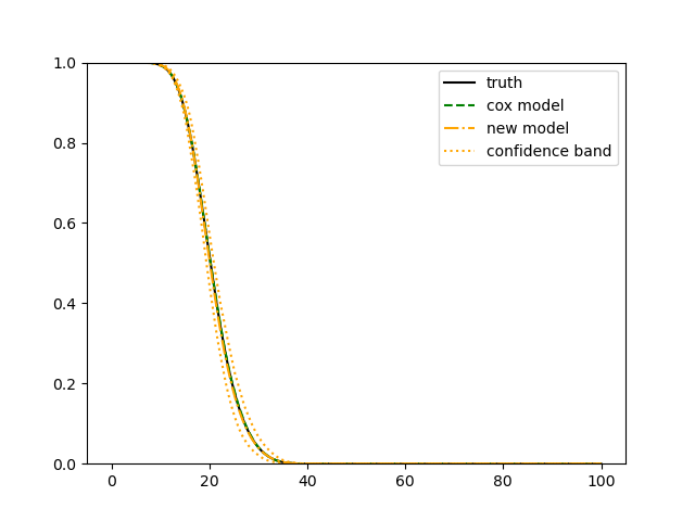
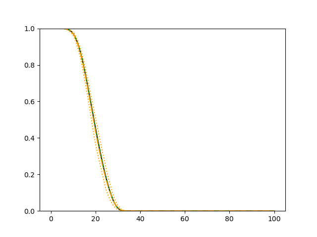
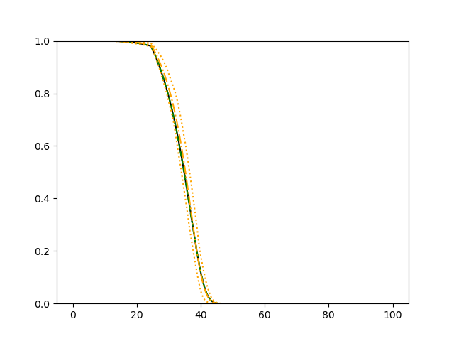
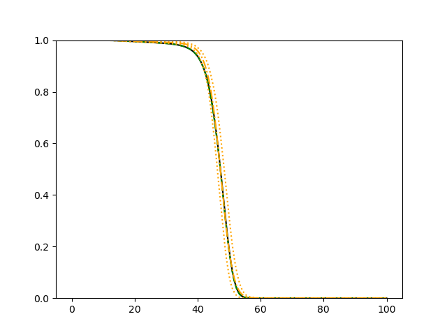
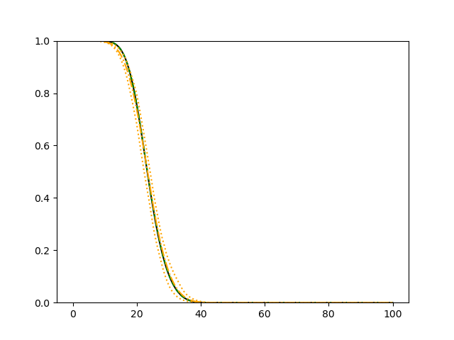
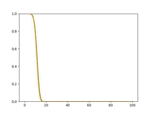
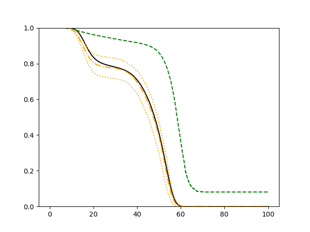
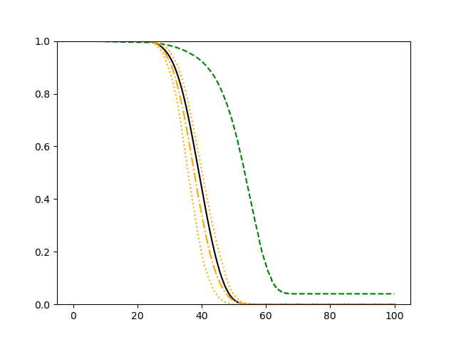
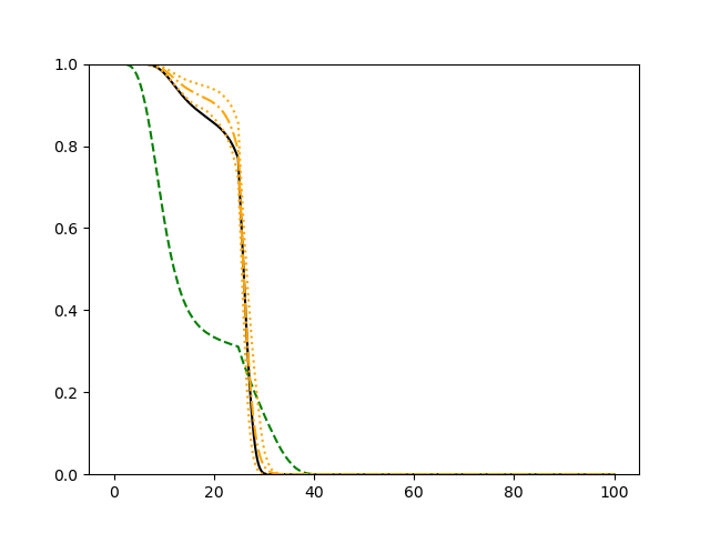
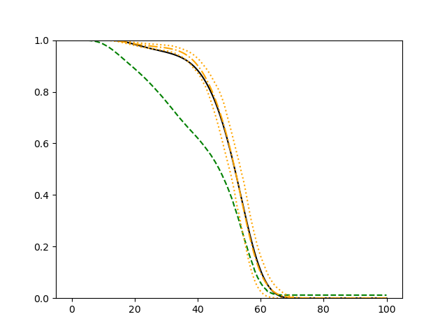
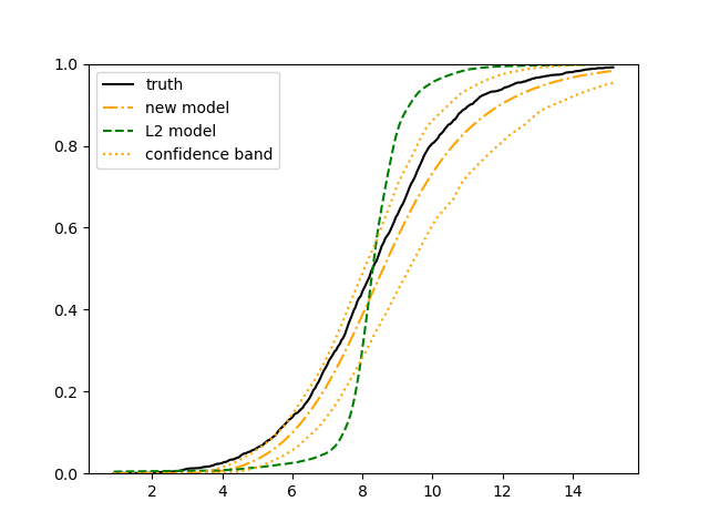
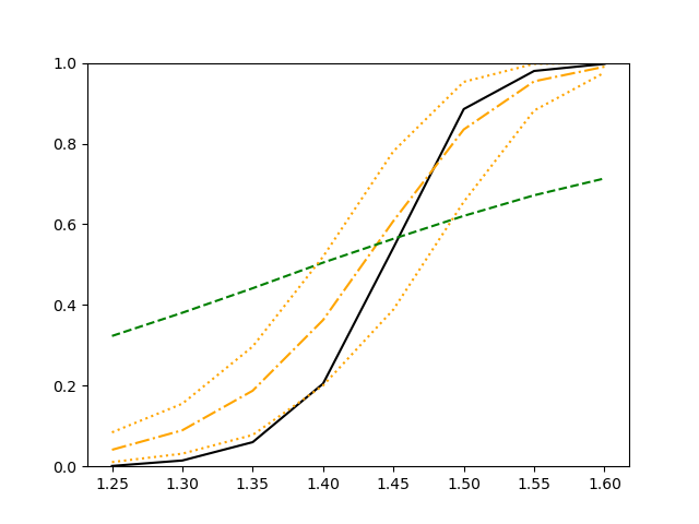
For each simulation setup, we independently generate a training set and a validation set with equal sample size, then fit our model using neural networks . We refit the model by swapping training and validation sets, and take the average as our estimator. For the Cox regression, we maximize the partial likelihood using all data. We repeat the process for $N$ independent data sets, and calculate the average and sample variance of these $N$ estimates at each time point on the fine grid for another set of randomly generated covariates. Finally, we plot the sample average of conditional survival curves estimated by neural networks together with the empirical confidence band, the average conditional survival curves estimated from the Cox regression, and the true conditional survival curve for a comparison.

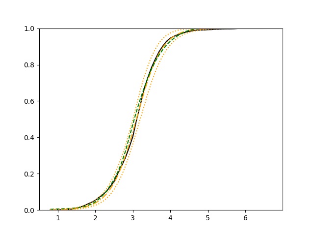
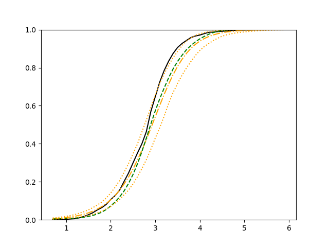
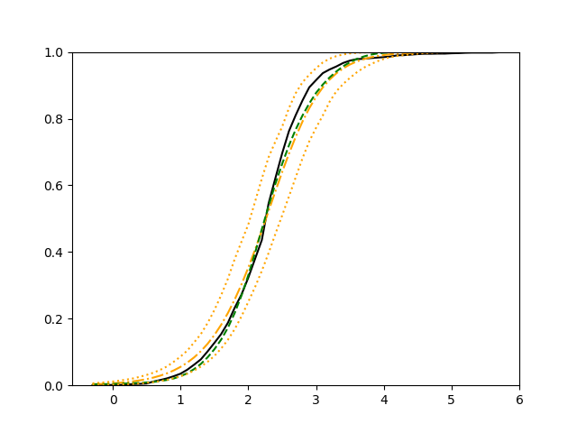
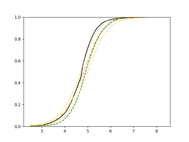
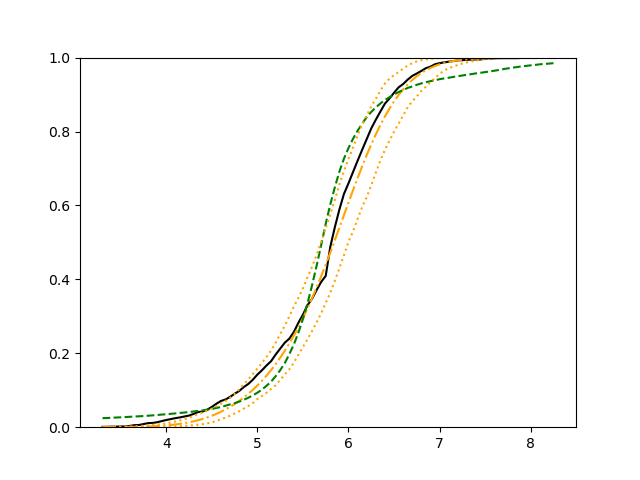
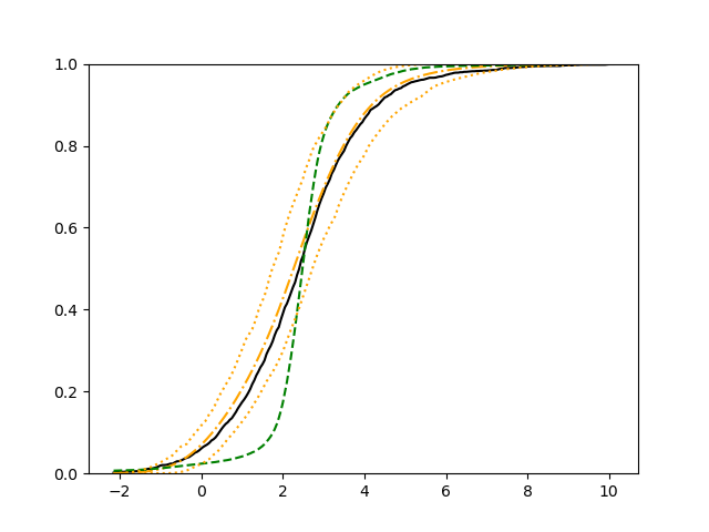
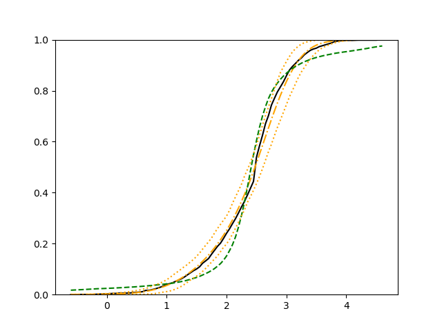
The simulation results illustrated in both Figure 2 and Figure 3 are based on a sample size of $n=3000$ (1500 for training and 1500 for validation) with 100 repetitions, where the curves for 9 different sets of covariates are presented. The green dashed line is the average estimated curve by using the partial likelihood method, the orange dash-dot line is the average estimated curve by our proposed neural networks method, and the black solid line is the truth curve. The dotted orange curves are the 90% confidence band obtained from the 100 repeated simulation runs using the proposed method. From Figure 2 we see that when the Cox model is correctly specified, both the partial likelihood method and our proposed neural networks method perform well, with estimated survival curves nicely overlapping with the corresponding true curves. When the Cox model is misspecified, Figure 3 shows that the partial likelihood approach yields severe biases, whereas the proposed neural networks method still works well with a similar performance to that in Setup 1 shown in Figure 2 .

For uncensored continuous outcomes, the traditional neural networks method with the commonly used $L_{2}$ loss function gives the conditional mean estimator. Then the conditional distribution function given a set of covariate values can be estimated by shifting the center of the empirical distribution of training set residuals to the estimated conditional mean. This would yield a valid estimator under the assumption that the errors (outcomes subtract their conditional means) are i.i.d. and uncorrelated with conditional means. We will evaluate the impact of this widely imposed condition for the mean regression via simulations. On the other hand, an estimator of the conditional distribution function gives a conditional mean estimator as follows:

Thus, we will compare our method to the method with $L_{2}$ loss on the estimation of the conditional distribution function as well as the estimation of the conditional mean.

In the following simulation studies, we consider i.i.d. data generated from the following model:

$i=1,\dots,n$, where $x_{i}$ denotes the $i$-th vector of all covariates, $\epsilon_{i}$ is mean-zero given all covariates, and $g$ is a function of covariates, so $\epsilon_{i}g(x_{i})$ is the $i$-th error term with zero-mean. We consider two simulation setups. In the first setup, the error is uncorrelated with the mean and has constant variance. In the second setup, the error is correlated with the mean and has non-constant variance. We would expect our new method outperforms the method with $L_{2}$ loss since our loss function is based on the nonparametric likelihood function that is free of any model assumption. Specifically, covariate values $x_{1i},\dots,x_{5i}$ are generated from the following distributions:

And the two setups are:

• Setup 1 (uncorrelated error with constant variance): generate another covariate $x_{6i}\sim\rm{N}\,(1,1)$ independently, then generate $\epsilon_{i}\sim$ a mixture distribution of $\rm{N}\,(-2,1)$, $\rm{N}\,(0,1)$, and $0.5x_{6i}^{2}$ with mixture probabilities $(0.1,0.7,0.2)$, and let $g(x_{i})=c$, where $c$ is a constant.

• Setup 2 (correlated error with non-constant variance): generate another covariate $x_{6i}\sim{\rm N}\,(1+0.5x_{1i},0.75)$, such that

  $$\begin{pmatrix}x_{1i}\\ x_{6i}\end{pmatrix}\sim\rm{N}\left(\begin{pmatrix}0\\ 1\end{pmatrix},\begin{pmatrix}1&0.5\\ 0.5&1\end{pmatrix}\right),$$

  then generate $\epsilon_{i}\sim$ a mixture distribution of $\rm{N}\,(-2,1)$, $\rm{N}\,(0,1)$, and $0.5x_{6i}^{2}$ with mixture probabilities $(0.1,0.7,0.2)$, and let $g(x_{i})=cx_{1i}^{2}$, where $c$ is a constant.

Note that different values of constant $c$ yield different signal to noise ratios in both setups.

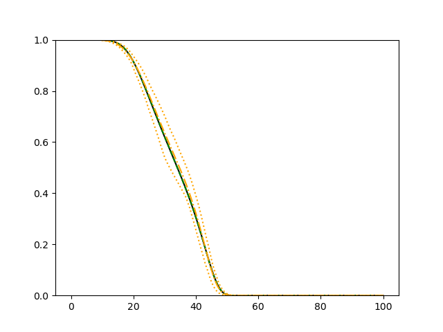
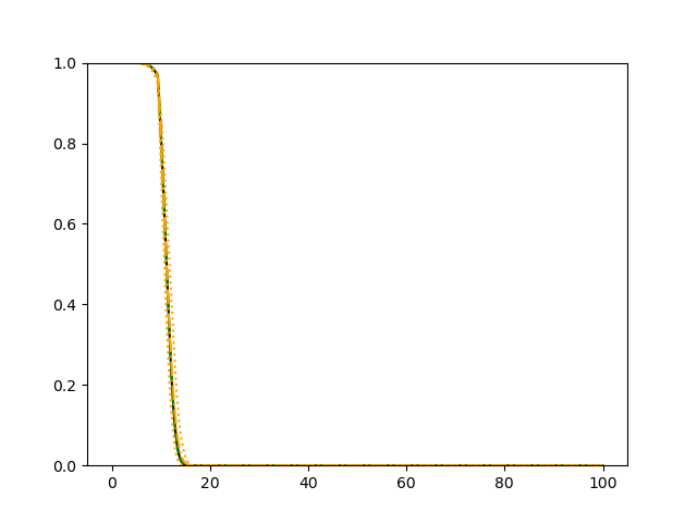
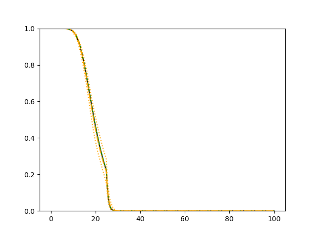
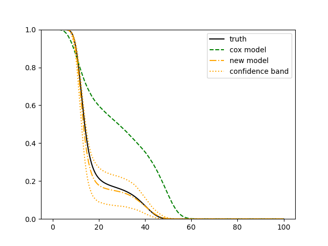
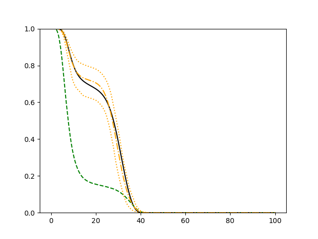
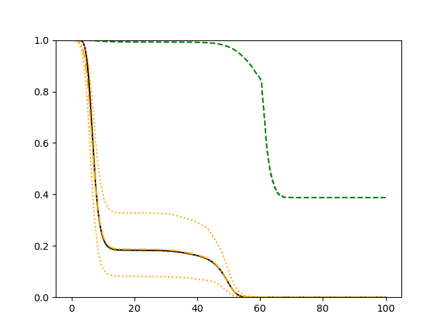
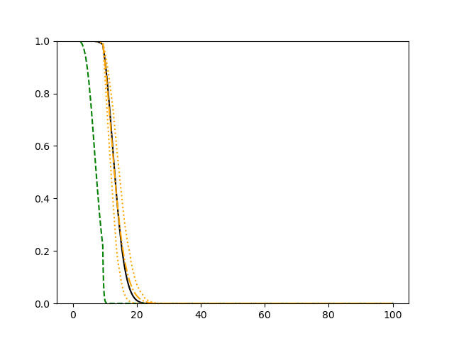
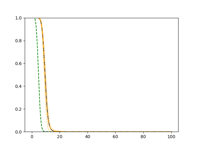
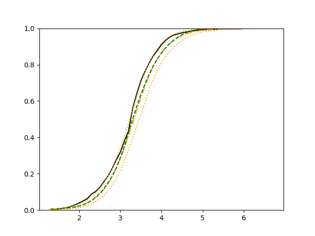
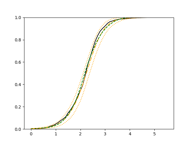
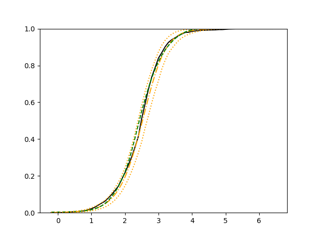
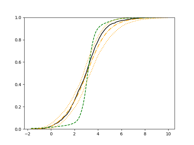
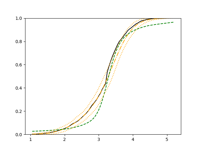
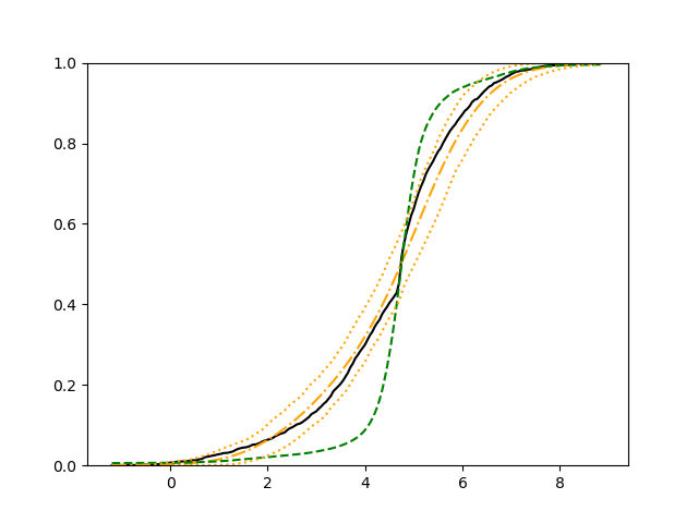
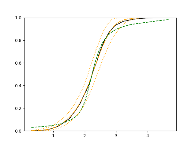
For each setup, we generate independent training and validation data sets with equal sample size, then fit both models with our general loss given in (6) and the $L_{2}$ loss using the same neural networks architecture. Figure 4 and Figure 5 illustrate the comparisons of estimated conditional distribution functions given 9 different sets of covariates between these two methods with a sample size of 5000 and 100 replications. In these figures, the black solid curve represents the true conditional distribution function, the green dashed curve represents the estimated conditional distribution function using $L_{2}$ loss, and the orange dash-dot curve represents the estimated conditional distribution using our method. The orange dotted curves are the 90% confidence band estimated using our method from the 100 repeated experiments. Figure 4 illustrates that when the error is uncorrelated with the covariates and has constant variance (Setup 1), both methods perform well in estimating the conditional distribution functions. When the error becomes correlated with the covariates and has non-constant variance (Setup 2), the traditional neural networks method using $L_{2}$ loss fails, which is illustrated in Figure 5.

We also compare the conditional mean estimates of both methods under two different sample sizes ($n=1000$ and $n=5000$) and two different magnitudes of noises ($c=0.5$ and $c=1$). We evaluate the performance of both methods by averaging the mean and median squared prediction errors, respectively, of 500 independently generated test data points over 100 replications, and summarize the results in Table 3. Coverage rates of 90% and 95% predictive intervals obtained using our method are also presented in Table 3. In Setup 1, both methods have similar mean squared prediction error, and our method yields slightly smaller median squared prediction error. In Setup 2, our model yields slightly better mean squared error, and significantly better median squared error. Our model provides reasonable prediction coverage rates in both setups, with improved performance as the sample size increases.

There are five real-world data sets analyzed by Kvamme et al. (2019). We re-analyze all these data sets using our method and compare with Kvamme et al. (2019), except one data set that contains too many ties for which a discrete survival model would be more appropriate. Theses four data sets are: the Study to Understand Prognoses Preferences Outcomes and Risks of Treatment (SUPPORT), the Molecular Taxonomy of Breast Cancer International Consortium (METABRIC), the Rotterdam tumor bank and German Breast Cancer Study Group (Rot.& GBSG), and the Assay Of Serum Free Light Chain (FLCHAIN).

The first three data sets are introduced and preprocessed by Katzman et al. (2018). The fourth data set is from the survival package of R (Therneau (2021)) and preprocessed by Kvamme et al. (2019). These four data sets have sample sizes of a few thousand and the covariate numbers range from 7 to 14. The covariates in these data sets are all time-independent.

To compare with their method, we use the same 5-fold cross-validated evaluation criteria described in Kvamme et al. (2019), including concordance index (C-index), integrated Brier score (IBS) and integrated binomial log-likelihood (IBLL). The time-dependent C-index (Antolini et al., 2005) estimates the probability that the predicted survival times of two comparable individuals have the same ordering as their true survival times,

The generalized Brier score (Graf et al., 1999) can be interpreted as the mean squared error of the probability estimates. To account for censoring, the scores are weighted by inverse censoring survival probability. In particular, for a fixed time $t$,

where $\widehat{G}(t)$ is the Kaplan-Meier estimate of the censoring time survival function. The binomial log-likelihood is similar to the Brier score,

The integrated Brier score IBS and the integrated binomial log-likelihood score IBLL are calculated by numerical integration over the time duration of the test set.

The results of our method are summarized in Table 4, together with the results of Kvamme et al. (2019) for a comparison. For SUPPORT and METABRIC data, our model yields the best integrated brier score and integrated binomial log-likelihood.

For Rot.&GBSG data, our model has the best C-index. The other results are comparable to that from the Kvamme et al. (2019). Note that in the 5-fold cross validation procedure, we use the set-aside data only as the test set for evaluation of the criteria and the rest of the data for training and validation of the neural networks, whereas Kvamme et al. (2019) use the set-aside data as both the test set and the validation set which would lead to more favorable evaluations.

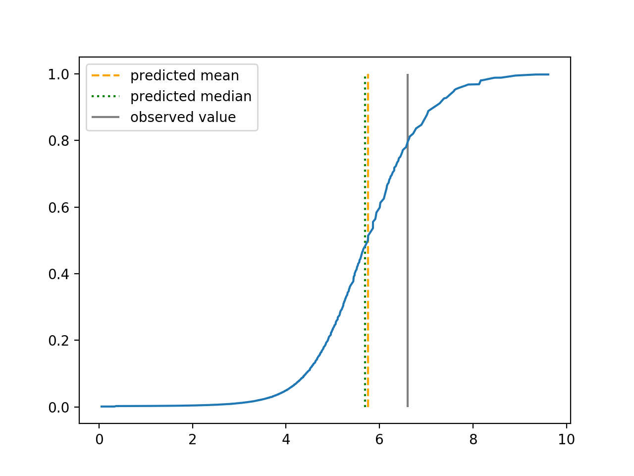
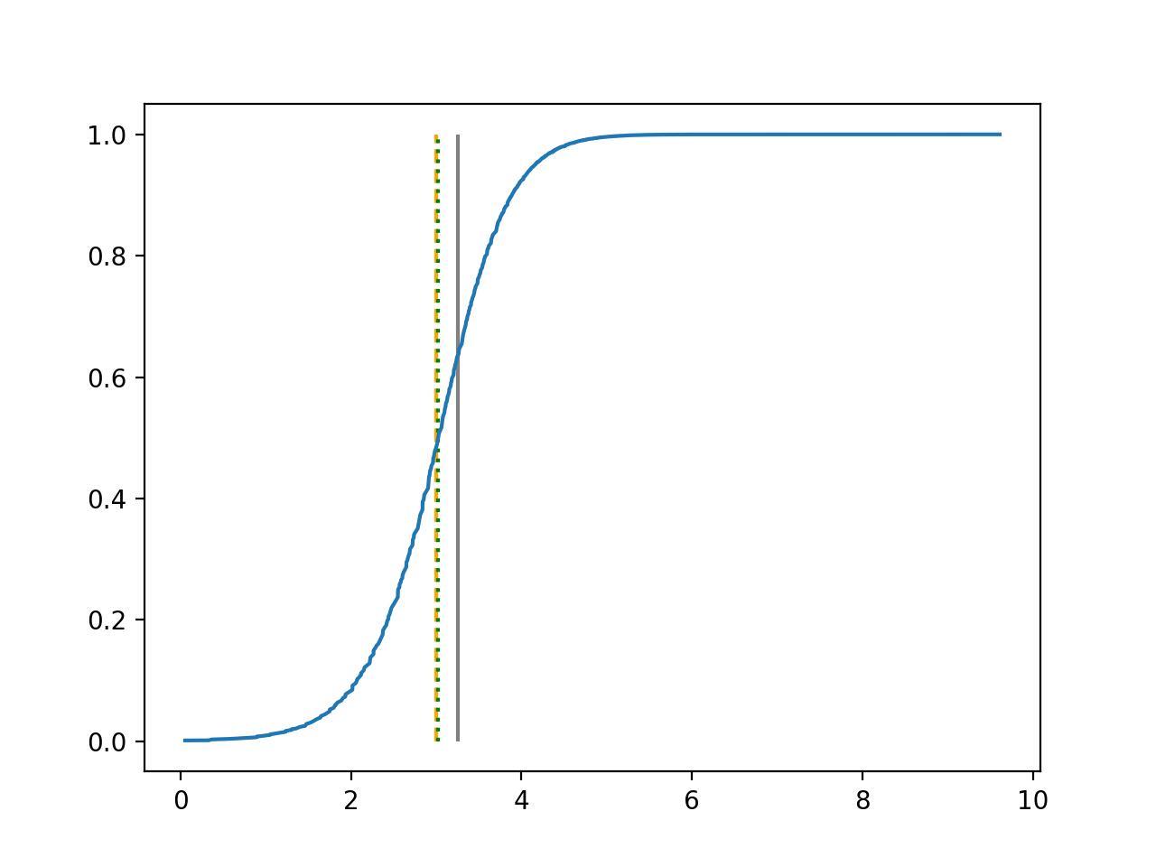
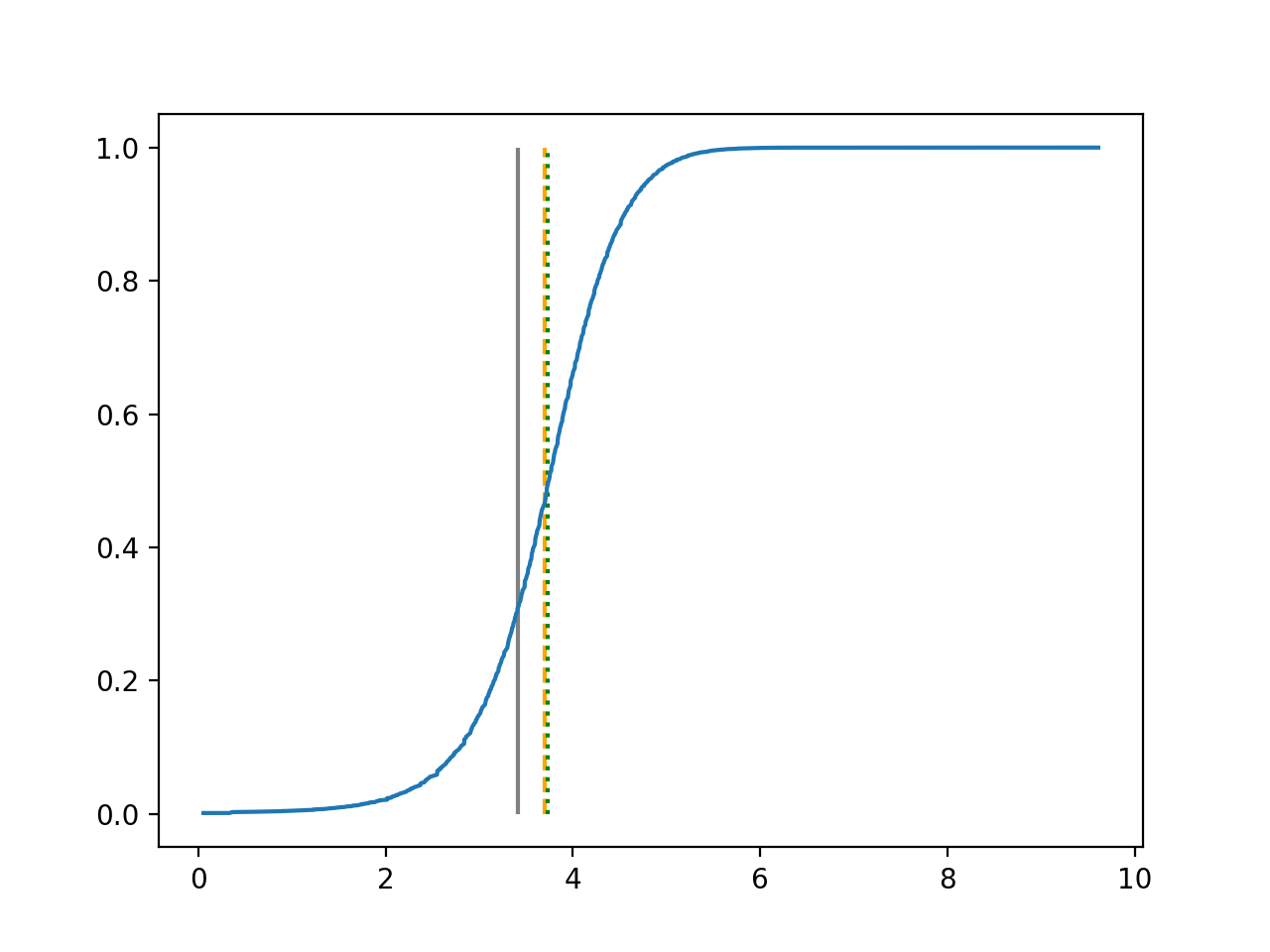
We use QSAR Fish Toxicity data set (Cassotti et al., 2015) for an illustration. This data set is collected for developing quantitative regression models to predict acute aquatic toxicity towards the fish Pimephales promelas (fathead minnow) on a set of 908 chemicals. Six molecular descriptors (representing the structure of chemical compounds) are used as the covariates and the concentration that causes death in 50% of test fish over a test duration of 96 hours, called $LC_{50}$ 96 hours (ranges from 0.053 to 9.612 with a mean of 4.064) was used as model response. The 908 data points are curated and filtered from experimental data. The six molecular descriptors come from a variable selection procedure through genetic algorithms. In their original research article, the authors used a $k$-nearest-neighbours (kNN) algorithm to estimate the mean. The data set can be obtained from the machine learning repository of the University of California, Irvine (https://archive.ics.uci.edu/ml/datasets/QSAR+fish+toxicity).

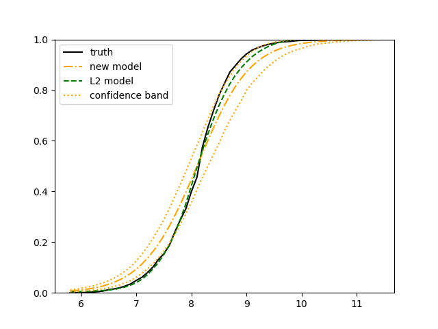
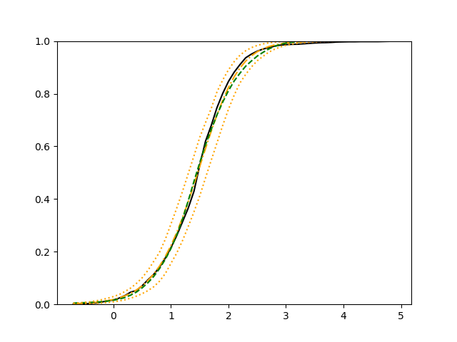
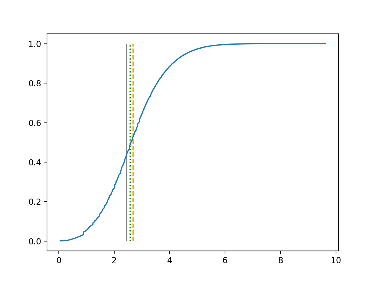
We use 5-fold cross-validated $R^{2}$, mean squared error and median squared error to evaluate our method and the neural networks with $L_{2}$ loss on this real-world data set and summarize the results in Table 5. Our new method yields better prediction in all three criteria. Note that we obtain the same 5-fold cross-validated $R^{2}$ value of 0.61 as Cassotti et al. (2015) did by using kNN. Predicted conditional distribution functions given four different sets of covariate values provided by our method are presented in Figure 6 for an illustration.

References

- Antolini et al. (2005) Laura Antolini, Patrizia Boracchi, and Elia M. Biganzoli. A time-dependent discrimination index for survival data. Statistics in medicine, 24 24:3927–44, 2005.
- Biganzoli et al. (1998) Elia Biganzoli, Patrizia Boracchi, Luigi Mariani, and Ettore Marubini. Feed forward neural networks for the analysis of censored survival data: a partial logistic regression approach. Statistics in Medicine, 17(10):1169–1186, 1998.
- Brown et al. (1997) Stephen F. Brown, Alan J. Branford, and William Moran. On the use of artificial neural networks for the analysis of survival data. IEEE Transactions on Neural Networks, 8(5):1071–1077, 1997.
- Cassotti et al. (2015) Matteo Cassotti, Davide Ballabio, Roberto Todeschini, and Viviana Consonni. A similarity-based qsar model for predicting acute toxicity towards the fathead minnow (pimephales promelas). SAR and QSAR in Environmental Research, 26(3):217–243, 2015.
- Ching et al. (2018) Travers Ching, Xun Zhu, and Lana X. Garmire. Cox-nnet: An artificial neural network method for prognosis prediction of high-throughput omics data. PLOS Computational Biology, 14(4):1–18, 04 2018.
- Chollet et al. (2015) Francois Chollet et al. Keras, 2015. URL https://github.com/fchollet/keras.
- Cox (1972) David R. Cox. Regression models and life-tables. Journal of the Royal Statistical Society: Series B (Methodological), 34(2):187–202, 1972.
- Faraggi and Simon (1995) David Faraggi and Richard Simon. A neural network model for survival data. Statistics in Medicine, 14(1):73–82, 1995.
- Gensheimer and Narasimhan (2019) Michael F. Gensheimer and Balasubramanian Narasimhan. A scalable discrete-time survival model for neural networks. PeerJ, 7:e6257–e6257, 01 2019.
- Giunchiglia et al. (2018) Eleonora Giunchiglia, Anton Nemchenko, and Mihaela van der Schaar. Rnn-surv: A deep recurrent model for survival analysis. pages 23–32, 2018.
- Goodfellow et al. (2016) Ian Goodfellow, Yoshua Bengio, and Aaron Courville. Deep Learning. MIT Press, 2016. http://www.deeplearningbook.org.
- Graf et al. (1999) Erika Graf, Claudia Schmoor, Willi Sauerbrei, and Martin Schumacher. Assessment and comparison of prognostic classification schemes for survival data. Statistics in medicine, 18 17-18:2529–45, 1999.
- Hall and Yao (2005) Peter Hall and Qiwei Yao. Approximating conditional distribution functions using dimension reduction. The Annals of Statistics, 33(3):1404–1421, 2005.
- Hall et al. (1999) Peter Hall, Rodney C. L. Wolff, and Qiwei Yao. Methods for estimating a conditional distribution function. Journal of the American Statistical Association, 94(445):154–163, 1999.
- Harrell et al. (1984) Frank E. Harrell, Kerry L. Lee, Robert M. Califf, David B. Pryor, and Robert A. Rosati. Regression modelling strategies for improved prognostic prediction. Statistics in medicine, 3(2):143—152, 1984.
- Kalbfleisch and Prentice (2002) John D. Kalbfleisch and Ross L. Prentice. The Statistical Analysis of Failure Time Data (2nd ed.). Hoboken, NJ:Wiley, 2002.
- Katzman et al. (2018) Jared L. Katzman, Uri Shaham, Alexander Cloninger, Jonathan Bates, Tingting Jiang, and Yuval Kluger. Deepsurv: personalized treatment recommender system using a cox proportional hazards deep neural network. BMC Medical Research Methodology, 18(1):24, 2018.
- Kingma and Ba (2014) Diederik P. Kingma and Jimmy Ba. Adam: A method for stochastic optimization. arXiv preprint, 2014. URL https://arxiv.org/abs/1412.6980.
- Kvamme et al. (2019) Håvard Kvamme, Ørnulf Borgan, and Ida Scheel. Time-to-event prediction with neural networks and cox regression. Journal of Machine Learning Research, 20(129):1–30, 2019.
- Solla et al. (1988) Sara A. Solla, Esther Levin, and Michael Fleisher. Accelerated learning in layered neural networks. Complex Syst., 2, 1988.
- Street (1998) Nick W. Street. A neural network model for prognostic prediction. In ICML, pages 540–546. Citeseer, 1998.
- Tang et al. (2022) Weijing Tang, Jiaqi Ma, Qiaozhu Mei, and Ji Zhu. Soden: A scalable continuous-time survival model through ordinary differential equation networks. Journal of Machine Learning Research, 23(34):1–29, 2022.
- Therneau (2021) Terry M. Therneau. A Package for Survival Analysis in R, 2021. URL https://CRAN.R-project.org/package=survival. R package version 3.2-13.
- Xiang et al. (2000) Anny Xiang, Pablo Lapuerta, Alex Ryutov, Jonathan Buckley, and Stanley Azen. Comparison of the performance of neural network methods and cox regression for censored survival data. Computational Statistics & Data Analysis, 34(2):243 – 257, 2000.