Conditional Normalizing flow for Monte Carlo sampling in lattice scalar field theory
Abstract
The cost of Monte Carlo sampling of lattice configurations is very high in the critical region of lattice field theory due to the high correlation between the samples. This paper suggests a Conditional Normalizing Flow (C-NF) model for sampling lattice configurations in the critical region to solve the problem of critical slowing down. We train the C-NF model using samples generated by Hybrid Monte Carlo (HMC) in non-critical regions with low simulation costs. The trained C-NF model is employed in the critical region to build a Markov chain of lattice samples with negligible autocorrelation. The C-NF model is used for both interpolation and extrapolation to the critical region of lattice theory. Our proposed method is assessed using the 1+1-dimensional scalar theory. This approach enables the construction of lattice ensembles for many parameter values in the critical region, which reduces simulation costs by avoiding the critical slowing down.
1 Introduction
In lattice field theory, Monte Carlo Simulation techniques are used to sample lattice configurations based on a distribution defined by the action of the lattice theory. The parameter value at which we generate the lattice samples determines the cost of the simulation. The non-critical region of the lattice theory has low simulation costs for algorithms like Hybrid Monte Carlo (HMC))[1]. However, as we attempt to sample uncorrelated lattice configurations from the critical region, the simulation cost increases rapidly. In the critical region, the integrated autocorrelation time, which gives the measure of correlation, increases rapidly and diverges at the critical point. For a finite-size lattice critical point corresponds to the peak point of the autocorrelation curve. This problem is known as the critical slowing down[2, 3]. Many efforts have been made to lessen the impact of critical slowing in statistical systems and lattice QFT [4, 5, 6]. But it always remains a challenging task to simulate near the critical point of a lattice QFT by overcoming the critical slowing down.
These days, ML-based solutions to this problem are becoming popular. Various ML algorithms have been applied for statistical physics and condensed matter problems[7, 8, 9, 10, 11, 12, 13, 14, 15, 16, 17, 18, 19] . Some generative learning algorithms[21, 22, 23, 24, 25, 26, 27] have recently been developed to avoid the difficulty in lattice field theory. Conditional GAN was used in a 2D lattice Gross Neveue model [20] and shown to be effective in mitigating the influence of critical slowdown. However, explicit probability density estimation is not accessible in GAN; thus, we cannot guarantee that the model distribution is identical to the true lattice distribution. Flow based generative leanings are found successful in avoiding the problem of critical slowing down in scalar field theory[21], fermionic system[22], U(1) gauge theory[24] and Schwinger models[26]. In the flow-based approach [21, 24] an NF model is trained at a single value of the action parameter with reverse KL divergence. Finally, the trained model can generate lattice samples at the same parameter value. This model is initialized from scratch for a parameter value and does not use any lattice samples. Since HMC simulation in the non-critical region is not affected by the critical slowing down problem, we can use samples from that region to train a generative model. We present a method for sampling lattice configurations near the critical regions using Conditional Normalizing Flow (C-NF) to reduce the problem of critical slowing down. This method involves training a C-NF model in a non-critical region to produce samples for several parameter values in the critical region. Our goal is to generate lattice configurations from the distribution , where denotes the lattice field, denotes the action parameter close to critical point and Z is the partition function. We train a C-NF model with HMC samples from for various non-critical values. We train the C-NF model to be a generalized model over parameters. The model is then interpolated or extrapolated to the values in the critical region to generate lattice configurations. However, the interpolated or extrapolated model may not directly provide samples from the true distribution. But the exactness can be guaranteed by using the Metropolis-Hastings(MH) algorithm at the end. So, after training, we use the interpolated/extrapolated model at critical region as proposal for constructing a Markov Chain via an independent MH algorithm[21]. This method is useful when the probability distribution is known up to a normalizing factor.
The primary contributions of this study are as follows:
-
1.
Using Conditional Normalizing Flows, we present a new method for sampling lattice configurations near the critical regions. This method eliminates the critical slowdown problem.
-
2.
The model has the ability to learn about the lattice system across multiple values and use this knowledge to generate sample at any given values. As a result, our model can generate samples at multiple values values in the critical region, which is not possible for the existing flow-based methods in lattice thoery.
-
3.
We also demonstrate that Conditional Normalizing flow can be used to do both interpolation and extrapolation for lattice theory. The extrapolation demonstrates the possibility of using our approach for sampling lattice gauge theory.
2 Lattice scalar Theory
In euclidean space, the action for theory can be written as:
| (1) |
where and are the two parameters of the theory.
On lattice the action become:
| (2) |
where is a discrete vector and represents two possible directions on the lattice. is defined on each lattice site, taking only real values.
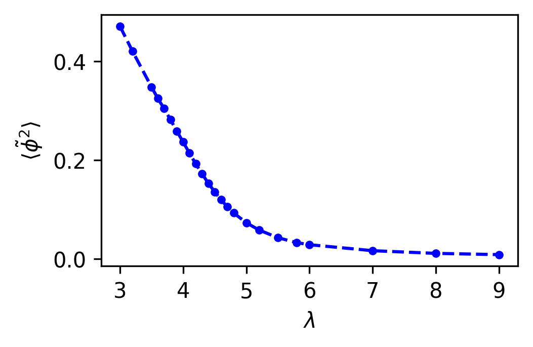
We choose this specific form of action for HMC simulation because it is suited for creating datasets for training the C-NF model. Using this form, we do not need to apply any further transformations to the samples during training. This action possesses symmetry, however it is spontaneously broken at a specific parameter region. We set for our numerical experiments and observed spontaneous symmetry breaking in the theory by varying . If we begin in the broken phase of the theory, the order parameter under consideration is nonzero which approaches zero at the critical point and remains zero in the symmetric phase, as shown in Figure 1. In HMC simulation we choose a parameter and produce configurations based on the probability distribution:
| (3) | |||
Each lattice configuration is a matrix with the dimensions . For our experiment, we use and add a periodic boundary condition to the lattice in all directions. More information on lattice theory can be found in ref. [28]. Some of the observables which we calculate on the lattice ensembles are:
-
1.
:
-
2.
Correlation Function:
Zero momentum Correlation Function:
-
3.
Two Point Susceptibility:
3 Conditional Normalizing Flow
Normalizing flows[29] are a generative model for constructing complex distributions by transforming a simple known distribution via a series of invertible and smooth mapping with inverse . If is the prior distribution and is the complex target distribution, then the model distribution can be written using the change of variable formula as
| (4) | |||
Fitting a flow-based model to a target distribution can be accomplished by minimising their KL divergence. The most crucial step is to build the flow so that we can calculate . One such method is the affine coupling block, which divides the input into two halves and applies an affine transformation to produce upper or lower triangular Jacobians. The transformation rules for such a building are as follows[30]:
| (5) |
where, represent element-wise product of two vectors.
The inverse of this coupling layer is simply computed as:
| (6) |
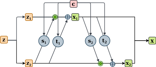
Because inverting an affine coupling layer does not require the inverse of , they can be any non-linear complex function and can thus be represented by neural networks. Introducing a conditioning parameter in NF is not as simple as it is in GAN. However, since and are only evaluated in the forward direction, we may concatenate the conditioning parameter with the input to the coupling layer in order to invert the model[31], as illustrated in Figure 2. As a result, the affine coupling transformation rules become:
| (7) |
And its inverse become
| (8) |
Let us designate the C-NF model as and its inverse as . The invertibility for any fixed condition is given by
| (9) |
The change of variable formula become
| (10) |
And the loss function is the KL divergence between the model distribution and target distribution :
| (11) |
We can find the maximum likelihood network parameter using this loss. Then, for a fixed , we can execute conditional generation of by sampling from and employing the inverted network .
4 Numerical Experiments
This section discusses dataset preparation and the model architecture utilized in training the C-NF model. In addition, the training details of the C-NF model and the sampling process in the critical region are discussed. We train the C-NF model with different datasets and model architecture for interpolation and extrapolation.
4.1 Dataset
In the non-critical region, we generate lattice configurations using HMC simulation where autocorrelation is low. In HMC simulation we use Molecular Dynamics(MD) step size=0.1 and MD trajectory length=1. For training purposes, we generate 10,000 lattice configurations for interpolation and 15,000 configurations for extrapolation of size for each value. In the critical region, for the evaluation purpose of the C-NF model, we use HMC to generate around lattice configurations per . This serves as a baseline for comparing observables to the observable produced through the proposed sampling strategy.
4.2 C-NF Model Architecture
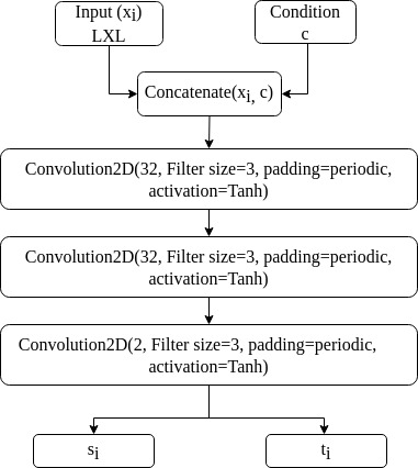
The affine coupling block displayed in Figure 2 is the fundamental building component of our C-NF model. For all neural networks and , we use the same architecture. Figure 3 depicts the neural networks used for and . In the neural networks, we solely employ Fully Convolutional Layers. For the first two layers, we use 64 filter for interpolation and 32 for extrapolation, all of which are in size. For each Convolutional layer, we employ the Tanh activation function. We use 8 such affine blocks while training for both interpolation and extrapolation. For each 8 affine block, the conditional parameter is concatenated with the input to and as shown in Figure 2.
4.3 Training and Sampling Procedure
The loss function used for training the C-NF model is the forward KL divergence as in Section 3 between the model distribution and target distribution :
| (12) | ||||
The expectation is evaluated using HMC samples from the non-critical region. During training, we maintain the learning rate at 0.0003 and employ the Adam optimizer.
Once training is complete, we invert the C-NF model, which we call the proposal model. The inputs to the proposal model are i) lattices from the Normal distribution and ii) as a conditional parameter for sample generation. Outputs are the lattice configurations and probability densities for each configuration for a given . For the critical region we give critical values as conditional parameter to the propsal model. We look at two scenarios in which a C-NF model can be either interpolated or extrapolated to the critical region. Both require different training, but the sampling technique is the same. The samples from the interpolated/extrapolated model may not exactly represent the true distribution of lattice theory . As a result, we use this model as a proposal for the independent MH algorithm, which generates a Markov Chain with asymptotic convergence to the true distribution.
4.4 Interpolation to the Critical Region
The set used to train the C-NF model for interpolation purposes is: . During training, we bypass the critical region [4.1-5.0] so that we can interpolate the model where the autocorrelation time is large for HMC simulation. We interpolate the trained model for multiple values belonging to the critical region (4.1, 4.2, 4.25, 4.3, 4.35, 4.4, 4.45, 4.5, 4.55, 4.6, 4.65, 4.7, 4.8, 5.0). For each values we generates one ensemble of configurations from the proposed method. On each ensemble we calculate different observables using bootstrap re-sampling method.
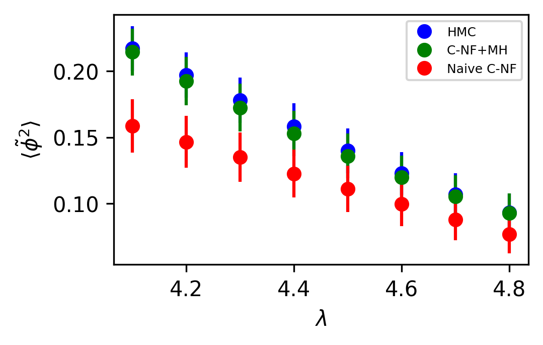
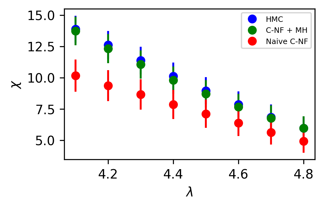
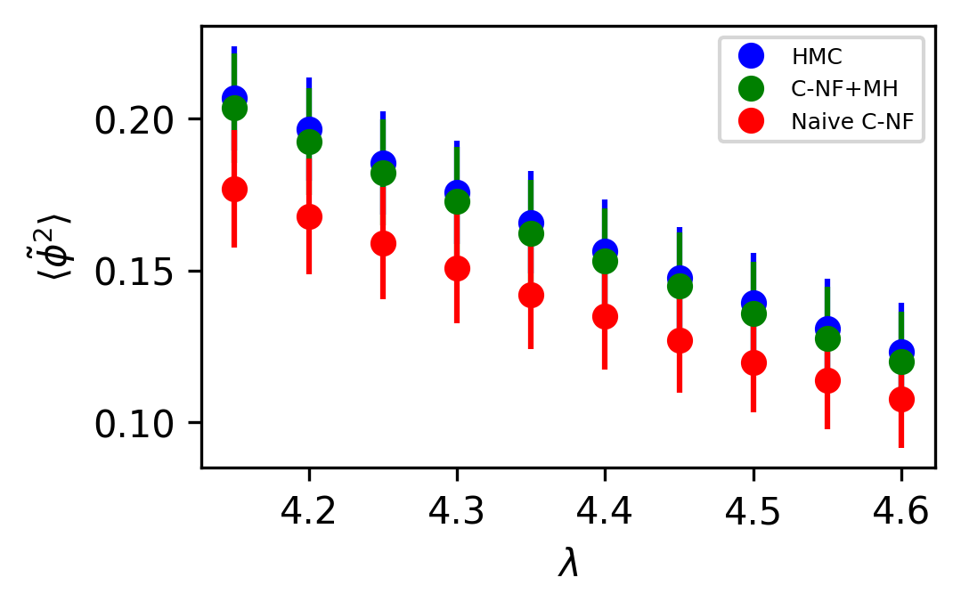
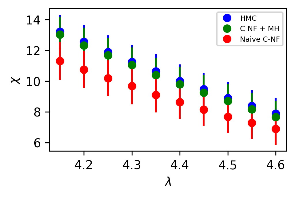
We compare the observables from HMC simulation and our proposed method. Observable from the Naive C-NF without MH is also shown to demonstrate the C-NF model’s proximity to the true distribution. In Figure 4 we plot two observables and for the interpolated values. Although the naive C-NF model has biases, MH can eliminate them, and both observables match pretty well within the statistical uncertainty. In the Appendix, we present a table of numerical values of the observables with errors.
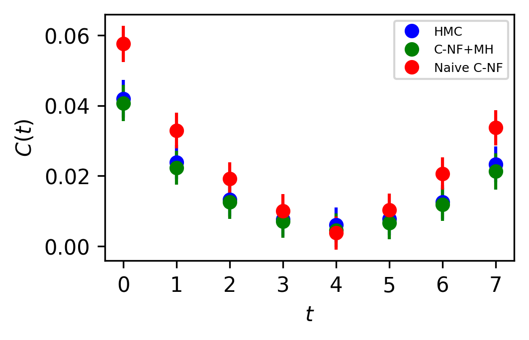
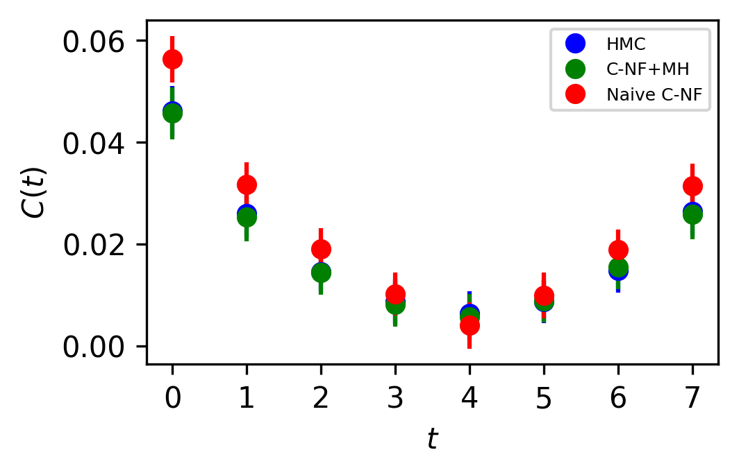
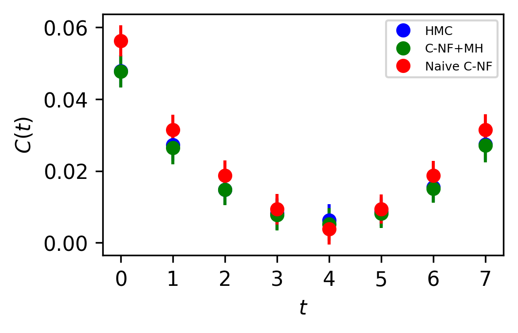
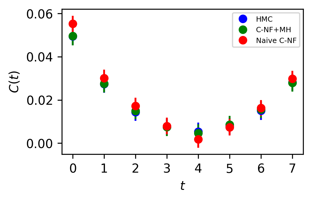
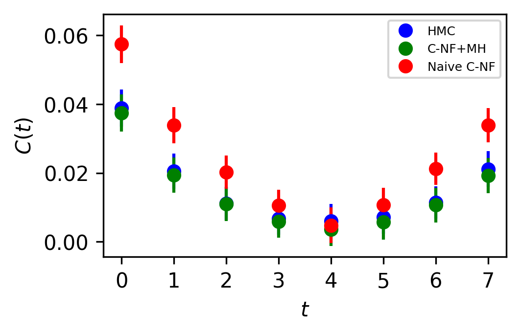
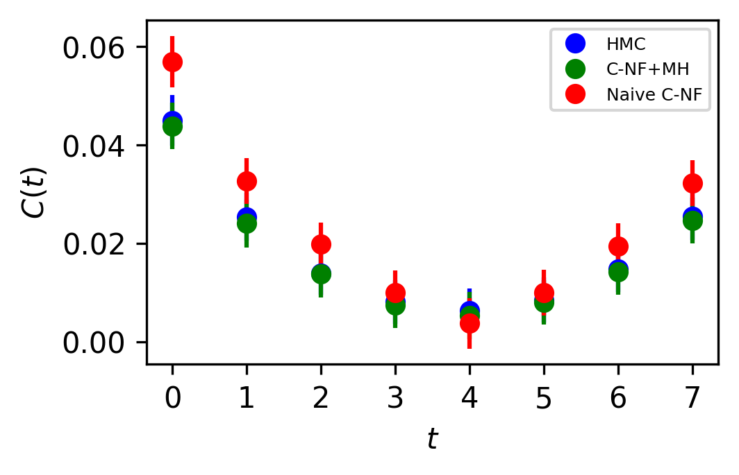
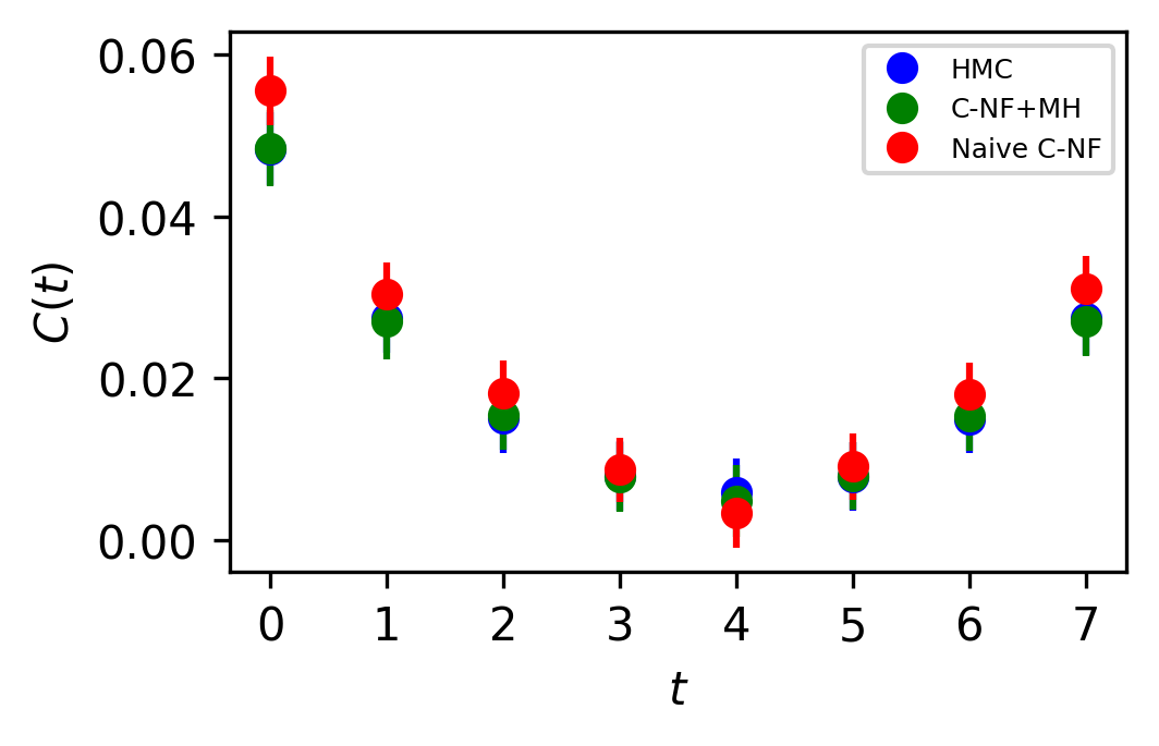
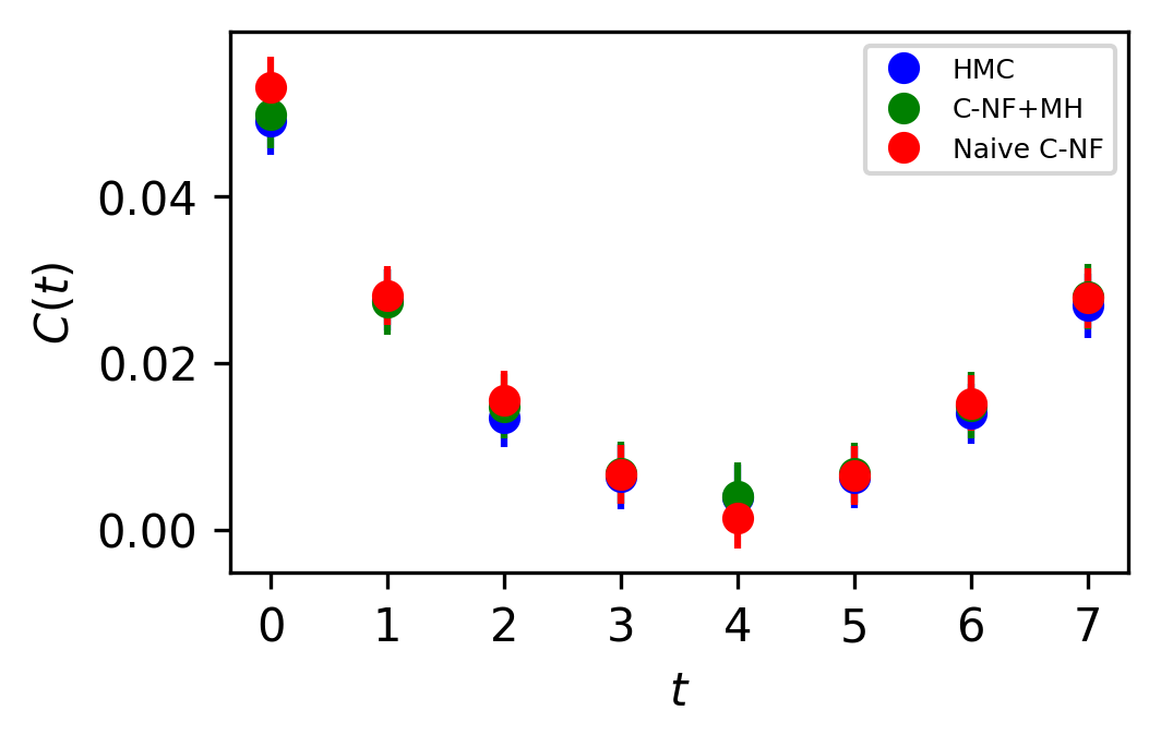
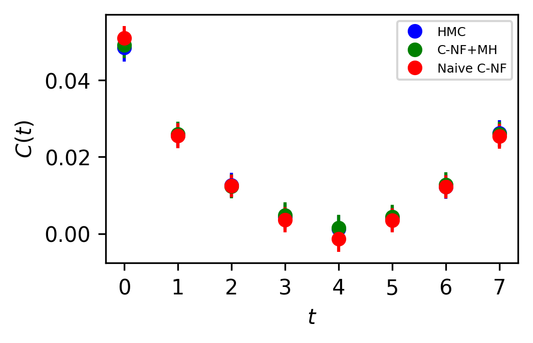
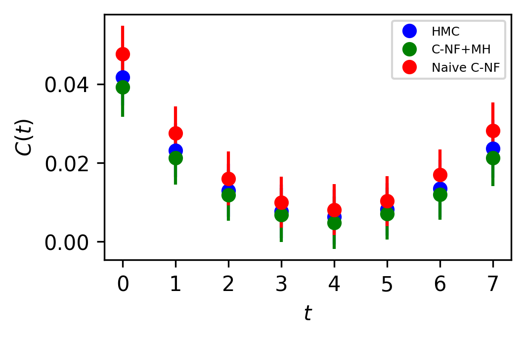
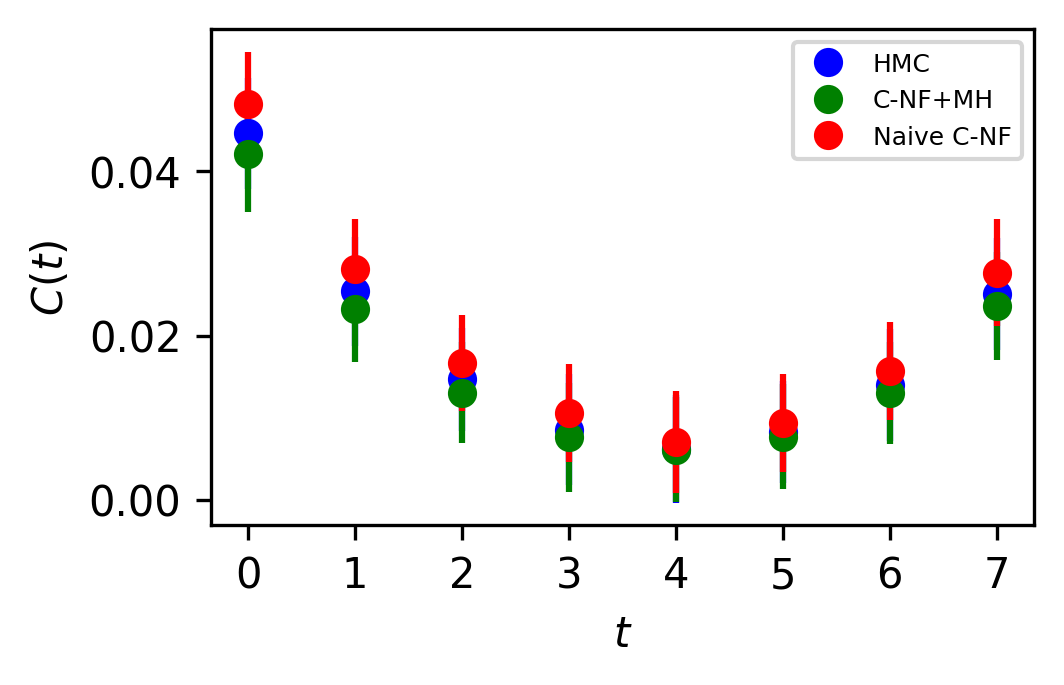
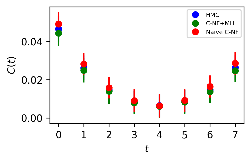
In Figure 5, the two point zero momentum correlation function is shown for four different values. For these values, we can observe that the correlation function is non-vanishing, which is a unique property of the critical region. The plots for other critical values are included in the Appendix.
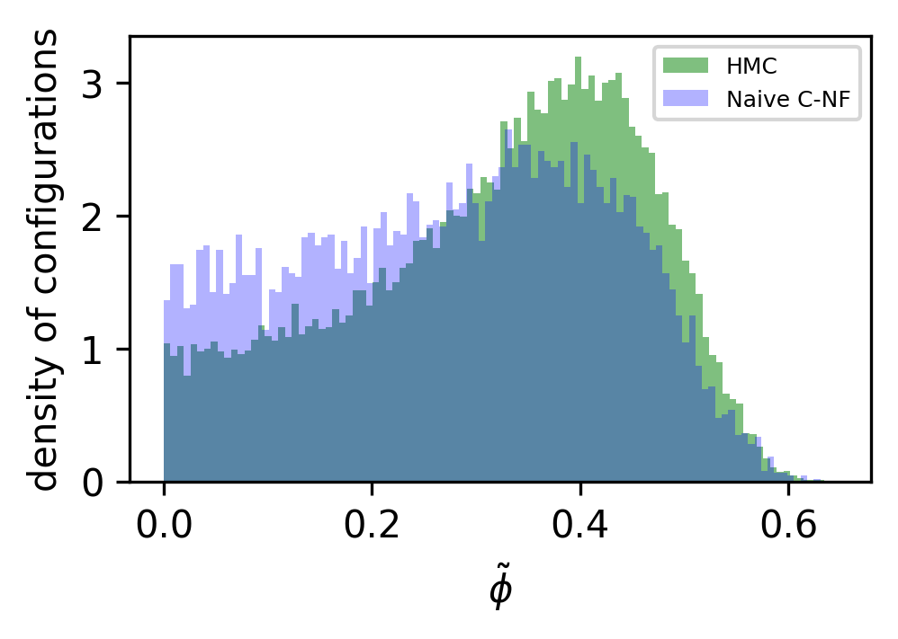
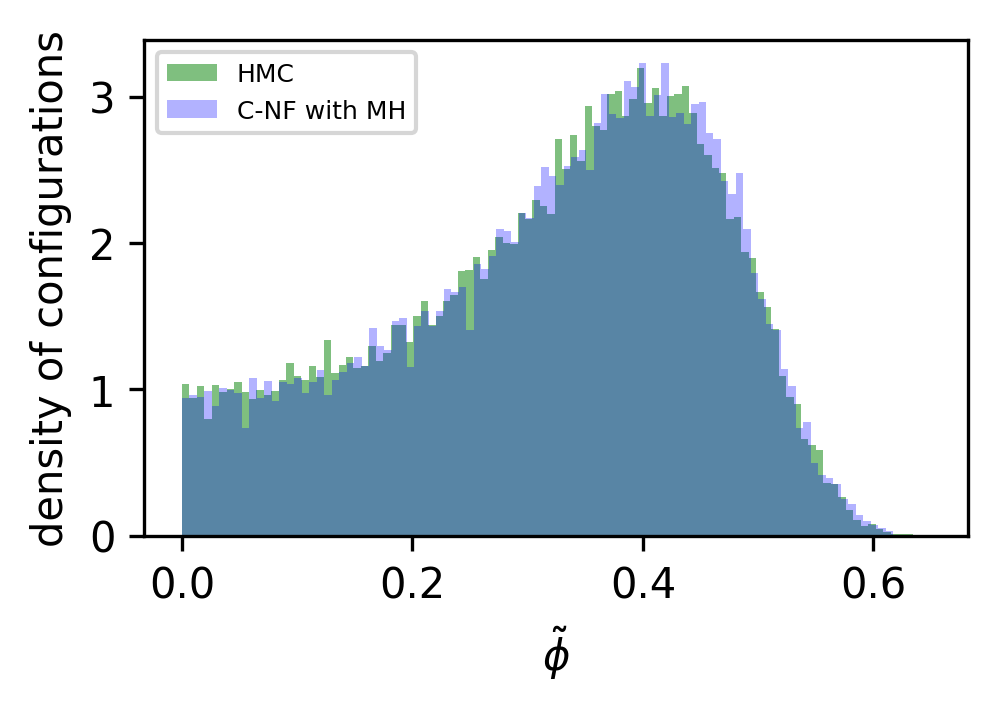
In Figure 6 we have also shown the histogram of for a particular critical . This demonstrates that MH can eliminate this kind artefacts created by the C-NF model.
We displayed plots of various observables on both phases around the critical point for the interpolation. We found that the observables estimated using our technique and the HMC match quite well.
4.5 Extrapolation to the Critical Region
The set used to train the C-NF model for the extrapolation is :. After training the model in the broken phase, we extrapolate it in the critical region around , which we take to be the critical region’s midpoint. The model is extrapolated for five distinct values:[4.2,4.3,4.4,4.5,4.6]. For each values we generates one ensemble of configurations from our method. Again, we calculate several observables for each ensemble using the bootstrap re-sampling method and compare them to the HMC results. We find that the size of the training dataset needs to be increased for extrapolation in order to achieve a C-NF model that is close to the true distribution in the broken phase. We plot the observables and in Figure 7 and the zero momentum correlation function is plotted in Figure 8 for four different in the critical region .

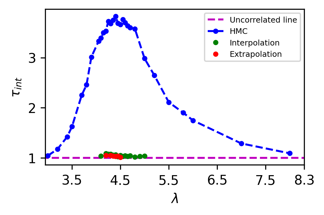
The naive C-NF model produces configurations that are inherently uncorrelated. Since we obtain a Markov Chain after applying MH, therefore we can’t guarantee the same. With a acceptance rate from the model, we see negligible correlation between the samples. The integrated autocorrelation time for from our proposed approach and HMC is plotted in Figure 9. It shows that we successfully reduce the Autocorrelation time for the Markov chain.The comparison is not absolute because HMC is affected by algorithmic settings. But we want to show that for the critical region, there is almost no correlation between samples in the Markov Chains obtained from both interpolation and extrapolation.
5 Cost Analysis
The sampling algorithm for the baseline approach (HMC) and the suggested method is vastly different; thus, a direct cost comparison is opaque. Nonetheless, we separate the simulation cost for the proposed technique into two components: Training time and sample generation time. On a Colab Tesla P100 GPU, the training time for the C-NF model for interpolation or extrapolation is roughly 5-6 hours. However, sample generation is very fast for the C-NF model. Generating one Markov Chain of configuration takes 5-7 minutes with a 25-40 acceptance rate. Due to the short generation time, a low acceptance rate is acceptable until the autocorrelation time increases.
Once the C-NF model has been trained, it can be employed repeatedly to generate configurations for a wide range of values. From a single training of the C-NF(interpolated) model, we have generated configurations for 13 ’s in the critical region. So, our approach outperforms HMC for sampling at multiple values in the critical region.
6 Conclusion
The critical slowing down problem prevents generating a large ensemble in the critical region of a lattice theory. In order to resolve this, we employ a Conditional normalizing flow trained on HMC samples with low autocorrelation and generate samples in the critical region. In order to learn a general distribution over parameter , we train the C-NF model away from the critical point of lattice theory. This model is interpolated in the critical region and serves as a proposal for the MH algorithm to generate a Markov chain. The degree to which the extrapolated or interpolated model resembles the actual distribution determines the acceptance rate in the critical region. In order to achieve a high acceptance rate and prevent the development of autocorrelation, the C-NF model must be trained adequately. The C-NF model generates uncorrelated samples, and we trained well enough to get 25-45 acceptance rate. With this much acceptance rate, we found no correlation between configuration in the Markov chain. As a result, our method significantly mitigates the critical slowing down problem. Aside from that, our method can be highly efficient when we need interpolation/extrapolation to numerous values in the critical region. Since lattice gauge theory requires extrapolation to the critical region, we have likewise extrapolated lattice theory to the critical region. We observe high agreement between observables estimated using the suggested technique and HMC simulation for both interpolation and extrapolation.
References
- [1] Simon Duane, Anthony D Kennedy, Brian J Pendleton, and Duncan Roweth. Hybrid monte carlo. Physics letters B, 195(2):216–222, 1987.
- [2] Ulli Wolff. CRITICAL SLOWING DOWN. Nucl. Phys. B Proc. Suppl., 17:93–102, 1990.
- [3] Stefan Schaefer, Rainer Sommer, and Francesco Virotta. Critical slowing down and error analysis in lattice QCD simulations. Nucl. Phys. B, 845:93–119, 2011.
- [4] Alberto Ramos. Playing with the kinetic term in the HMC. PoS, LATTICE2012:193, 2012.
- [5] Arjun Singh Gambhir and Kostas Orginos. Improved sampling algorithms in lattice qcd, 2015.
- [6] Michael G. Endres, Richard C. Brower, William Detmold, Kostas Orginos, and Andrew V. Pochinsky. Multiscale monte carlo equilibration: Pure yang-mills theory. Physical Review D, 92(11), Dec 2015.
- [7] Kai Zhou, Gergely Endrődi, Long-Gang Pang, and Horst Stöcker. Regressive and generative neural networks for scalar field theory. Phys. Rev. D, 100:011501, Jul 2019.
- [8] Dian Wu, Lei Wang, and Pan Zhang. Solving statistical mechanics using variational autoregressive networks. Phys. Rev. Lett., 122:080602, Feb 2019.
- [9] Jan M Pawlowski and Julian M Urban. Reducing autocorrelation times in lattice simulations with generative adversarial networks. Machine Learning: Science and Technology, 1(4):045011, oct 2020.
- [10] Kim A. Nicoli, Shinichi Nakajima, Nils Strodthoff, Wojciech Samek, Klaus-Robert Müller, and Pan Kessel. Asymptotically unbiased estimation of physical observables with neural samplers. Physical Review E, 101(2), feb 2020.
- [11] Juan Carrasquilla. Machine learning for quantum matter. Advances in Physics: X, 5(1):1797528, jan 2020.
- [12] Junwei Liu, Huitao Shen, Yang Qi, Zi Yang Meng, and Liang Fu. Self-learning monte carlo method and cumulative update in fermion systems. Physical Review B, 95(24), jun 2017.
- [13] Johanna Vielhaben and Nils Strodthoff. Generative neural samplers for the quantum heisenberg chain. Physical Review E, 103(6), jun 2021.
- [14] Chuang Chen, Xiao Yan Xu, Junwei Liu, George Batrouni, Richard Scalettar, and Zi Yang Meng. Symmetry-enforced self-learning monte carlo method applied to the holstein model. Physical Review B, 98(4), jul 2018.
- [15] Giacomo Torlai and Roger G. Melko. Learning thermodynamics with boltzmann machines. Phys. Rev. B, 94:165134, Oct 2016.
- [16] G. Carleo and M. Troyer. Solving the quantum many-body problem with artificial neural networks. Science, 355:602, 2017.
- [17] Lei Wang. Discovering phase transitions with unsupervised learning. Phys. Rev. B, 94:195105, Nov 2016.
- [18] Pengfei Zhang, Huitao Shen, and Hui Zhai. Machine learning topological invariants with neural networks. Phys. Rev. Lett., 120:066401, Feb 2018.
- [19] Japneet Singh, Mathias Scheurer, and Vipul Arora. Conditional generative models for sampling and phase transition indication in spin systems. SciPost Physics, 11(2), Aug 2021.
- [20] Ankur Singha, Dipankar Chakrabarti, and Vipul Arora. Generative learning for the problem of critical slowing down in lattice Gross Neveu model. arXiv: 2111.00574, 2021.
- [21] M. S. Albergo, G. Kanwar, and P. E. Shanahan. Flow-based generative models for markov chain monte carlo in lattice field theory. Phys. Rev. D, 100:034515, Aug 2019.
- [22] Michael S. Albergo, Gurtej Kanwar, Sébastien Racanière, Danilo J. Rezende, Julian M. Urban, Denis Boyda, Kyle Cranmer, Daniel C. Hackett, and Phiala E. Shanahan. Flow-based sampling for fermionic lattice field theories. 2021.
- [23] Phiala E Shanahan, Daniel Trewartha, and William Detmold. Machine learning action parameters in lattice quantum chromodynamics. Physical Review D, 97(9):094506, 2018.
- [24] Gurtej Kanwar, Michael S. Albergo, Denis Boyda, Kyle Cranmer, Daniel C. Hackett, Sébastien Racanière, Danilo Jimenez Rezende, and Phiala E. Shanahan. Equivariant flow-based sampling for lattice gauge theory. Physical Review Letters, 125(12), Sep 2020.
- [25] Michael S. Albergo, Denis Boyda, Daniel C. Hackett, Gurtej Kanwar, Kyle Cranmer, Sébastien Racanière, Danilo Jimenez Rezende, and Phiala E. Shanahan. Introduction to normalizing flows for lattice field theory, 2021.
- [26] Michael S. Albergo, Denis Boyda, Kyle Cranmer, Daniel C. Hackett, Gurtej Kanwar, Sébastien Racanière, Danilo J. Rezende, Fernando Romero-López, Phiala E. Shanahan, and Julian M. Urban. Flow-based sampling in the lattice Schwinger model at criticality. 2 2022.
- [27] Daniel C. Hackett, Chung-Chun Hsieh, Michael S. Albergo, Denis Boyda, Jiunn-Wei Chen, Kai-Feng Chen, Kyle Cranmer, Gurtej Kanwar, and Phiala E. Shanahan. Flow-based sampling for multimodal distributions in lattice field theory. 7 2021.
- [28] Ingmar Vierhaus. Simulation of phi 4 theory in the strong coupling expansion beyond the ising limit. Master’s thesis, Humboldt-Universität zu Berlin, Mathematisch-Naturwissenschaftliche Fakultät I, 2010.
- [29] Danilo Jimenez Rezende and Shakir Mohamed. Variational inference with normalizing flows, 2015.
- [30] Lynton Ardizzone, Carsten Lüth, Jakob Kruse, Carsten Rother, and Ullrich Köthe. Guided image generation with conditional invertible neural networks, 2019.
- [31] Lynton Ardizzone, Carsten Lüth, Jakob Kruse, Carsten Rother, and Ullrich Köthe. Guided image generation with conditional invertible neural networks. CoRR, abs/1907.02392, 2019.
7 Appendix
| HMC | C-NF with MH | Naive C-NF | HMC | C-NF with MH | Naive C-NF | |
| 4.10 | ||||||
| 4.20 | ||||||
| 4.25 | ||||||
| 4.30 | ||||||
| 4.35 | ||||||
| 4.40 | ||||||
| 4.45 | ||||||
| 4.50 | ||||||
| 4.60 | ||||||
| 4.65 | ||||||
| 4.70 | ||||||
| 4.8 | ||||||
| 5.0 | ||||||
| 4.1 | 4.2 | 4.3 | 4.4 | 4.5 | 4.6 | 4.7 | 4.8 | 4.9 | 5.0 | |
| 1.033 | 1.084 | 1.071 | 1.059 | 1.048 | 1.039 | 1.041 | 1.018 | 1.030 | 1.037 |
| 4.2 | 4.3 | 4.4 | 4.5 | 4.6 | |
| 1.046 | 1.049 | 1.027 | 1.032 | 1.010 |
| HMC | C-NF with MH | Naive C-NF | HMC | C-NF with MH | Naive C-NF | |
| 4.20 | ||||||
| 4.30 | ||||||
| 4.40 | ||||||
| 4.50 | ||||||
| 4.60 | ||||||