∎
National University of Singapore
Tel.: +65-6516-8473
Fax: +65-6872-3939
22email: statsll@nus.edu.sg 33institutetext: Aishwarya Bhaskaran 44institutetext: Department of Statistics and Applied Probability
National University of Singapore
Tel.: +65-6601-6229
Fax: +65-6872-3939
44email: staai@nus.edu.sg 55institutetext: David J. Nott 66institutetext: Department of Statistics and Applied Probability
National University of Singapore
Tel.: +65-6516-2744
Fax: +65-6872-3939
66email: standj@nus.edu.sg
Conditionally structured variational Gaussian approximation with importance weights††thanks: Linda Tan and Aishwarya Bhaskaran are supported by the start-up grant R-155-000-190-133.
Abstract
We develop flexible methods of deriving variational inference for models with complex latent variable structure. By splitting the variables in these models into “global” parameters and “local” latent variables, we define a class of variational approximations that exploit this partitioning and go beyond Gaussian variational approximation. This approximation is motivated by the fact that in many hierarchical models, there are global variance parameters which determine the scale of local latent variables in their posterior conditional on the global parameters. We also consider parsimonious parametrizations by using conditional independence structure, and improved estimation of the log marginal likelihood and variational density using importance weights. These methods are shown to improve significantly on Gaussian variational approximation methods for a similar computational cost. Application of the methodology is illustrated using generalized linear mixed models and state space models.
Keywords:
Gaussian variational approximation Sparse precision matrix Stochastic variational inference Importance weighted lower bound Rényi’s divergence1 Introduction
In many modern statistical applications, it is necessary to model complex dependent data. In these situations, models which employ observation specific latent variables such as random effects and state space models are widely used because of their flexibility, and Bayesian approaches dealing naturally with the hierarchical structure are attractive in principle. However, incorporating observation specific latent variables leads to a parameter dimension increasing with sample size, and standard Bayesian computational methods can be challenging to implement in very high-dimensional settings. For this reason, approximate inference methods are attractive for these models, both in exploratory settings where many models need to be fitted quickly, as well as in applications involving large datasets where exact methods are infeasible. One of the most common approximate inference paradigms is variational inference (Ormerod and Wand, 2010; Blei et al., 2017), which is the approach considered here.
Our main contribution is to consider partitioning the unknowns in a local latent variable model into “global” parameters and “local” latent variables, and to suggest ways of structuring the dependence in a variational approximation that match the specification of these models. We go beyond standard Gaussian approximations by defining the variational approximation sequentially, through a marginal density for the global parameters and a conditional density for local parameters given global parameters. Each term in our approximation is Gaussian, but we allow the conditional covariance matrix for the local parameters to depend on the global parameters, which leads to an approximation that is not jointly Gaussian. We are particularly interested in improved inference on global variance and dependence parameters which determine the scale and dependence structure of local latent variables. With this objective, we suggest a parametrization of our conditional approximation to the local variables that is well-motivated and respects the exact conditional independence structure in the true posterior distribution. Our approximations are parsimonious in terms of the number of required variational parameters, which is important since a high-dimensional variational optimization is computationally burdensome. The methods suggested improve on Gaussian variational approximation methods for a similar computational cost. Besides defining a novel and useful variational family appropriate to local latent variable models, we also employ importance weighted variational inference methods (Burda et al., 2016; Domke and Sheldon, 2018) to further improve the quality of inference, and elaborate further on the connections between this approach and the use of Rényi’s divergence within the variational optimization (Li and Turner, 2016; Regli and Silva, 2018; Yang et al., 2019).
Our method is a contribution to the literature on the development of flexible variational families, and there are many interesting existing methods for this task. One fruitful approach is based on normalizing flows (Rezende and Mohamed, 2015), where a variational family is defined using an invertible transformation of a random vector with some known density function. To be useful, the transformation should have an easily computed Jacobian determinant. In the original work of Rezende and Mohamed (2015), compositions of simple flows called radial and planar flows were considered. Later authors have suggested alternatives, such as autoregressive flows (Germain et al., 2015), inverse autoregressive flows (Kingma et al., 2016), and real-valued non-volume preserving transformations (Dinh et al., 2017), among others. Spantini et al. (2018) gives a theoretical framework connecting Markov properties of a target posterior distribution to representations involving transport maps, with normalizing flows being one way to parametrize such mappings. The variational family we consider here can be thought of as a simple autoregressive flow, but carefully constructed to preserve the conditional independence structure in the true posterior and to achieve parsimony in the representation of dependence between local latent variables and global scale parameters. Our work is also related to the hierarchically structured approximations considered in Salimans and Knowles (2013, Section 7.1); these authors also consider other flexible approximations based on mixture models, and a variety of innovative numerical approaches to the variational optimization. Hoffman and Blei (2015) propose an approach called structured stochastic variational inference which is applicable in conditionally conjugate models. Their approach is similar to ours, in the sense that local variables depend on global variables in the variational posterior. However conditional conjugacy does not hold in the examples we consider.
The methods we describe can be thought of as extending the Gaussian variational approximation (GVA) of Tan and Nott (2018), where parametrization of the variational covariance matrix was considered in terms of a sparse Cholesky factor of the precision matrix. Similar approximations have been considered for state space models in Archer et al. (2016). The sparse structure reduces the number of free variational parameters, and allows matching the exact conditional independence structure in the true posterior. Tan (2018) propose an approach called reparametrized variational Bayes, where the model is reparametrized by applying an invertible affine transformation to the local variables to minimize their posterior dependency on global variables, before applying a mean field approximation. The affine transformation is obtained by considering a second order Taylor series approximation to the posterior of the local variables conditional on the global variables. One way of improving on Gaussian approximations is to consider mixtures of Gaussians (Jaakkola and Jordan, 1998; Salimans and Knowles, 2013; Miller et al., 2016; Guo et al., 2016). However, even with a parsimonious parametrization of component densities, a large number of additional variational parameters are added with each mixture component. Other flexible variational families can be formed using copulas (Tran et al., 2015; Han et al., 2016; Smith et al., 2019), hierarchical variational models (Ranganath et al., 2016) or implicit approaches (Huszár, 2017).
We specify the model and notation in Section 2 and introduce the conditionally structured Gaussian variational approximation (CSGVA) in Section 3. The algorithm for optimizing the variational parameters is described in Section 4 and Section 5 highlights the association between GVA and CSGVA. Section 6 describes how CSGVA can be improved using importance weighting. Experimental results and applications to generalized linear mixed models (GLMMs) and state space models are presented in Sections 7, 8 and 9 respectively. Section 10 gives some concluding discussion.
2 Model specification and notation
Let be observations from a model with global variables and local variables , where contains latent variables specific to for . Suppose is a vector of length and each is a vector of length . Let . We consider models where the joint density is of the form
The observations are conditionally independent given and . Conditional on , the local variables form a th order Markov chain if , and they are conditionally independent if . This class of models include important models such as GLMMs and state space models. Next, we define some mathematical notation before discussing CSGVA for this class of models.
2.1 Notation
For an matrix , let denote the diagonal elements of and be the diagonal matrix obtained by setting non-diagonal elements in to zero. Let be the vector of length obtained by stacking the columns of under each other from left to right and be the vector of length obtained from by eliminating all superdiagonal elements of . Let be the elimination matrix, be the commutation matrix and be the duplication matrix (see Magnus and Neudecker, 1980). Then , , if is lower triangular, and if is symmetric. Let be a vector of ones of length . The Kronecker product between any two matrices is denoted by . Scalar functions applied to vector arguments are evaluated element by element. Let d denote the differential operator (see e.g. Magnus and Neudecker, 1999).
3 Conditionally structured Gaussian variational approximation
We propose to approximate the posterior distribution of the model defined in Section 2 by a density of the form
where , , and and are the precision (inverse covariance) matrices of and respectively. Here and depend on , but we do not denote this explicitly for notational conciseness. Let and be unique Cholesky factorizations of and respectively, where and are lower triangular matrices with positive diagonal entries. We further define and to be lower triangular matrices of order and respectively such that and if for . The purpose of introducing and is to allow unconstrained optimization of the variational parameters in the stochastic gradient ascent algorithm, since diagonal entries of and are constrained to be positive. Note that and also depend on but again we do not show this explicitly in our notation.
As depends on , the joint distribution is generally non-Gaussian even though and are individually Gaussian. Here we consider a first order approximation and assume that and are linear functions of :
| (1) |
In (1), is a vector of length , is a matrix, is a vector of length and is a matrix. For this specification, is not jointly Gaussian due to dependence of the covariance matrix of on . It is Gaussian if and only if . The set of variational parameters to be optimized is denoted as
As motivation for the linear approximation in (1), consider the linear mixed model,
where is a vector of responses of length for the th subject, and are covariate matrices of dimensions and respectively, is a vector of coefficients of length and are random effects. Assume is known. Then the global parameters consists of and . The posterior of conditional on is
Thus , where is a normal density with precision matrix and mean . The precision matrix depends on linearly and the mean depends on linearly after scaling by the covariance matrix. The linear approximation in (1) tries to mimic this dependence relationship.
The proposed variational density is conditionally structured and highly flexible. Such dependence structure is particularly valuable in constructing variational approximations for hierarchical models, where there are global scale parameters in which help to determine the scale of local latent variables in the conditional posterior of . While marginal posteriors of the global variables are often well approximated by Gaussian densities, marginal posteriors of the local variables tend to exhibit more skewness and kurtosis. This deviation from normality can be captured by , which is a mixture of normal densities. The formulation in (1) also allows for a reduction in the number of variational parameters if conditional independence structure consistent with that in the true posterior is imposed on the variational approximation.
3.1 Using conditional independence structure
Tan and Nott (2018) incorporate the conditional independence structure of the true posterior into Gaussian variational approximations by using the fact that zeros in the precision matrix correspond to conditional independence for Gaussian random vectors. This incorporation achieves sparsity in the precision matrix of the approximation and leads to a large reduction in the number of variational parameters to be optimized. For high-dimensional , this sparse structure is especially important because a full Gaussian approximation involves learning a covariance matrix where the number of elements grows quadratically with the dimension of .
Recall that . Suppose is conditionally independent of in the posterior for , given and . For instance, in a GLMM, may be subject specific random effects, and these are conditionally independent given the global parameters, so this structure holds with . In the case of a state space model for a time series, are the latent states and this structure holds with . Note that ordering of the latent variables is important here.
Now partition the precision matrix of into blocks with row and column partitions corresponding to . Let be the block corresponding to horizontally and vertically for . If is conditionally independent of for , given and , then we set for all pairs with . Let denote the indices of elements in which are fixed at zero by this conditional independence requirement. If we choose and for all and all in (1), then has the same block sparse structure we desire for the lower triangular part of . By Proposition 1 of Rothman et al. (2010), this means that will have the desired block sparse structure. Hence we impose the constraints and for and all , which reduces the number of variational parameters to be optimized.
4 Optimization of variational parameters
To make the dependence on explicit, write as . The variational parameters are optimized by minimizing the Kullback-Leibler divergence between and the true posterior , where
Minimizing is therefore equivalent to maximizing an evidence lower bound on the log marginal likelihood , where
| (2) |
In (2), denotes expectation with respect to . We seek to maximize with respect to using stochastic gradient ascent. Starting with some initial estimate of , we perform the following update at each iteration ,
where represents a small stepsize taken in the direction of the stochastic gradient . The sequence should satisfy the conditions and (Spall, 2003).
An unbiased estimate of the gradient can be constructed using (2) by simulating from . However, this approach usually results in large fluctuations in the stochastic gradients. Hence we implement the “reparametrization trick” (Kingma and Welling, 2014; Rezende et al., 2014; Titsias and Lázaro-Gredilla, 2014), which helps to reduce the variance of the stochastic gradients. This approach writes as a function of the variational parameters and a random vector having a density not depending on . To explain further, let , where and are vectors of length and corresponding to and respectively. Consider a transformation of the form
| (3) |
Since and are functions of from (1),
Hence and are functions of , and is a function of both and . This transformation is invertible since given and , we can first recover , find and , and then recover . Applying this transformation,
| (4) | ||||
where denotes expectation with respect to and .
4.1 Stochastic gradients
Next, we differentiate (4) with respect to to find unbiased estimates of the gradients. As depends on directly as well as through , applying the chain rule, we have
| (5) | ||||
| (6) |
Note that = 0 as it is the expectation of the score function. Roeder et al. (2017) refer to the expressions inside the expectations in (5) and (6) as the total derivative and path derivative respectively. In (6), the contributions to the gradient from and cancel each other if approximates the true posterior well (at convergence). However, the score function is not necessarily small even if is a good approximation to . This term affects adversely the ability of the algorithm to converge and “stick” to the optimal variational parameters, a phenomenon Roeder et al. (2017) refers to as “sticking the landing”. Hence we consider the path derivative,
| (7) |
as an unbiased estimate of the true gradient . Tan and Nott (2018) and Tan (2018) also demonstrate that the path derivative has smaller variation about zero when the algorithm is close to convergence.
Let , where and are vectors of length and respectively corresponding to the partitioning of . Then is given by
where
Here and are diagonal matrices of order and respectively such that for . Formally, and . The full expression and derivation of are given in Appendix A. In addition, we show (in Appendix A) that
is model specific and we discuss the application to GLMMs and state space models in Sections 8 and 9 respectively.
4.2 Stochastic variational algorithm
The stochastic gradient ascent algorithm for CSGVA is outlined in Algorithm 1. For computing the stepsize, we use Adam (Kingma and Ba, 2015), which uses bias-corrected estimates of the first and second moments of the stochastic gradients to compute adaptive learning rates.
Initialize , , ,
For ,
-
1.
Generate and compute .
-
2.
Compute gradient .
-
3.
Update biased first moment estimate:
. -
4.
Update biased second moment estimate:
. -
5.
Compute bias-corrected first moment estimate:
. -
6.
Compute bias-corrected second moment estimate:
. -
7.
Update .
At iteration , the variational parameter is updated as . Let denote the stochastic gradient estimate at iteration . In steps 3 and 4, Adam computes estimates of the mean (first moment) and uncentered variance (second moment) of the gradients using exponential moving averages, where control the decay rates. In step 4, is evaluated as , where denotes the Hadamard (element-wise) product. As and are initialized as zero, these moment estimates tend to be biased towards zero, especially at the beginning of the algorithm if , are close to one. As ,
where if for . Otherwise, can be kept small since the weights for past gradients decrease exponentially. An analogous argument holds for . Thus the bias can be corrected by using the estimates and in steps 5 and 6. The change is then computed as
where controls the magnitude of the stepsize and is a small positive constant which ensures that the denominator is positive. In our experiments, we set , , and , values close to what is recommended by Kingma and Ba (2015).
At each iteration , we can also compute an unbiased estimate of the lower bound,
where is computed in step 1. Since these estimates are stochastic, we follow the path traced by , which is an average of the lower bounds averaged over every 1000 iterations, as a means to diagnose the convergence of Algorithm 1. tends to increase monotonically at the start, but as the algorithm comes close to convergence, the values of fluctuate close to and about the true maximum lower bound. Hence, we fit a least squares regression line to the past values of and terminate Algorithm 1 once the gradient of the regression line becomes negative (see Tan, 2018). For our experiments, we set .
5 Links to Gaussian variational approximation
CSGVA is an extension of Gaussian variational approximation (GVA, Tan and Nott, 2018). In both approaches, the conditional posterior independence structure of the local latent variables is used to introduce sparsity in the precision matrix of the approximation. Below we demonstrate that GVA is a special case of CSGVA when .
Tan and Nott (2018) consider a GVA of the form
Note that and are lower triangular matrices. Using a vector , we can write
Assuming for CSGVA, we have from (3) that
where . Hence we can identify
If the standard way of initializing of Algorithm 1 (by setting ) does not work well, we can use this association to initialize Algorithm 1 by using the fit from GVA. This informative initialization can reduce computation time significantly although there may be a risk of getting stuck in a local mode.
6 Importance weighted variational inference
Here we discuss how CSGVA can be improved by maximizing an importance weighted lower bound (IWLB, Burda et al., 2016), which leads to a tighter lower bound on the log marginal likelihood, and a variational approximation less prone to underestimation of the true posterior variance. We also relate the IWLB with Rényi’s divergence (Rényi, 1961; van Erven and Harremos, 2014) between and , demonstrating that maximizing the IWLB instead of the usual evidence lower bound leads to a transition in the behavior of the variational approximation from “mode-seeking” to “mass-covering”. We first define Rényi’s divergence and the variational Rényi bound (Li and Turner, 2016), before introducing the IWLB as the expectation of a Monte Carlo approximation of the variational Rényi bound.
6.1 Rényi’s divergence and variational Rényi bound
Rényi’s divergence provides a measure of the distance between two densities and , and it is defined as
for , . This definition can be extended by continuity to the orders 0, 1 and , as well as to negative orders . Note that is no longer a divergence measure if , but we can write as for by the skew symmetry property. As approaches 1, the limit of is the Kullback-Leibler divergence, . In variational inference, minimizing the Kullback-Leibler divergence between the variational density and the true posterior is equivalent to maximizing a lower bound on the log marginal likelihood due to the relationship:
Generalizing this relation using Rényi’s divergence measure, Li and Turner (2016) define the variational Rényi bound as
Note that , the limit of as , is equal to . A Monte Carlo approximation of when the expectation is intractable is
| (8) |
where is a set of samples generated randomly from , and
are importance weights. For each , . The limit of as is . Hence is an unbiased estimate of as , where denotes expectation with respect to . For , is not an unbiased estimate of .
6.2 Importance weighted lower bound
The importance weighted lower bound (IWLB, Burda et al., 2016) is defined as
where in (8). It reduces to when . By Jensen’s inequality,
Thus provides a lower bound to the log marginal likelihood for any positive integer . From Theorem 6.1 (Burda et al., 2016), this bound becomes tighter as increases.
Theorem 6.1
increases with and approaches as if is bounded.
Proof
Let be selected randomly without replacement from . Then for any , where denotes the expectation associated with the randomness in selecting given . Thus
If is bounded, then as by the law of large numbers. Hence as .
Next, we present some properties of Rényi’s divergence and which are important in understanding the behavior of the variational density arising from maximizing . The proofs of these properties can be found in van Erven and Harremos (2014) and Li and Turner (2016).
Property 1
is increasing in , and is continuous in on .
Property 2
is continuous and decreasing in for fixed .
Theorem 6.2
There exists for given and such that
Proof
From Property 2,
From Property 1, since is continuous and decreasing for , there exists such that .
Minimizing Rényi’s divergence for tends to produce approximations which are mode-seeking (zero-forcing) while maximizing Rényi’s divergence for encourages mass-covering behavior. Theorem 6.2 suggests that maximizing the IWLB results in a variational approximation whose Rényi’s divergence from the true posterior can be captured with , which represents a mix and certain balance between mode-seeking and mass-covering behavior (Minka, 2005). In our experiments, we observe that maximizing the IWLB is highly effective in correcting the underestimation of posterior variance in variational inference.
Alternatively, if we approximate by considering a second-order Taylor expansion of about , where , and then take expectations, we have
Maddison et al. (2017) and Domke and Sheldon (2018) provide bounds on the order of the remainder term in the Taylor approximation above, and demonstrate that the “looseness” of the IWLB is given by as . Minimizing is equivalent to minimizing the divergence . Note that if has thin tails compared to , then the variance of will be large. Hence minimizing attempts to match with so that is able to cover the tails.
6.3 Unbiased gradient estimate of importance weighted lower bound
To maximize the IWLB in CSGVA, we need to find an unbiased estimate of using the transformation in (3). Let , for , and .
| (9) | ||||
where and for are normalized importance weights. Applying chain rule,
| (10) |
In Section 4.1, we note that as it is the expectation of the score function and hence we can omit to obtain an unbiased estimate of . However, in this case, it is unclear if
| (11) |
Roeder et al. (2017) conjecture that (11) is true and report improved results when omitting the term from in computing gradient estimates. However, Tucker et al. (2018) demonstrated via simulations that (11) does not hold generally and that such omission will result in biased gradient estimates. Our own simulations using CSGVA also suggest that (11) does not hold even though omission of does lead to improved results. As the stochastic gradient algorithm is not guaranteed to converge with biased gradient estimates, we turn to the double reparametrized gradient estimate proposed by Tucker et al. (2018) which allows unbiased gradient estimates to be constructed with the omission of albeit with revised weights.
Since depends on directly as well as through , we use chain rule to obtain
| (12) | ||||
where
Alternatively,
| (13) | ||||
Comparing (12) and (13), we have
Combining the above expression with (9) and (10), we find that
An unbiased gradient estimate is thus given by
Thus, to use CSGVA with important weights, we only need to modify Algorithm 1 by drawing samples in step 1 instead of a single sample and then compute the unbiased gradient estimate, , in step 2. The rest of the steps in Algorithm 1 remain unchanged. In the importance weighted version of CSGVA, the gradient estimate based on a single sample is replaced by a weighted sum of the gradients in (7) based on samples . However, these weights do not necessarily sum to 1. An unbiased estimate of itself is given by .
7 Experimental results
We apply CSGVA to GLMMs and state space models and compare the results with that of GVA in terms of computation time and accuracy of the posterior approximation. Lower bounds reported exclude constants which are independent of the model variables. We also illustrate how CSGVA can be improved using importance weighting (IW-CSGVA), considering . We find that IW-CSGVA performs poorly if it is initialized in the standard manner using . This is because, when is still far from optimal, a few of the importance weights tend to dominate with the rest close to zero, thus producing inaccurate estimates of the gradients. Hence we initialize IW-CSGVA using the CSGVA fit, and the algorithm is terminated after a short run of 1000 iterations as IW-CSGVA is computationally intensive and improvements in the IWLB and variational approximation seem to be negligible thereafter. Posterior distributions estimated using MCMC via RStan are regarded as the ground truth. Code for all variational algorithms are written in Julia and are available as supplementary materials. All experiments are run on on Intel Core i9-9900K CPU @3.60 GHz with 16GB RAM. As the computation time of IW-CSGVA increases linearly with , we also investigate the speedup that can be achieved through parallel computing on a machine with 8 cores. Julia retains one worker (or core) as the master process and parallel computing is implemented using the remaining seven workers.
The parametrization of a hierarchical model plays a major role in the rate of convergence of both GVA and CSGVA. In some cases, it can even affect the ability of the algorithm to converge (to a local mode). We have attempted both the centered and noncentered parametrizations (Papaspiliopoulos et al., 2003, 2007), which are known to have a huge impact on the rate of convergence of MCMC algorithms. These two parametrizations are complementary and neither is superior to the other. If an algorithm converges slowly under one parametrization, it often converges much faster under the other. Which parametrization works better usually depends on the nature of data. For the datasets that we use in the experiments, the centered parametrization was found to have better convergence properties than the noncentered parametrization for GLMMs while the noncentered parametrization is preferred for stochastic volatilty models. These observations are further discussed below.
8 Generalized linear mixed models
Let denote the vector of responses of length for the th subject for , where is generated from some distribution in the exponential family. The mean is connected to the linear predictor via
for some smooth invertible link function . The fixed effects is a vector and is a vector of random effects specific to the th subject. and are vectors of covariates of length and respectively. Let , and . We focus on the one-parameter exponential family with canonical links. This includes the Bernoulli model, Bern(), with the logit link and the Poisson model, Pois(), with the log link . Let be the unique Cholesky decomposition of , where is a lower triangular matrix with positive diagonal entries. Define such that and if , and let . We consider normal priors, and , where and are set as 100.
The above parametrization of the GLMM is noncentered since has mean 0. Alternatively, we can consider the centered parametrization proposed by Tan and Nott (2013). Suppose the covariates for the random effects are a subset of the covariates for the fixed effects and the first column of and are ones corresponding to an intercept and random intercept respectively. Then we can write
where . We further split into covariates which are subject specific (varies only with and assumes the same value for ) and those which are not, and accordingly, where , are vectors of length and respectively. Then
where
Let . The centered parametrization is represented as
| (14) |
for .
Tan and Nott (2013) compare the centered, noncentered and partially noncentered parametrizations for GLMMs in the context of variational Bayes, showing that the choice of parametrization affects not only the rate of convergence, but also the accuracy of the variational approximation. For CSGVA, we observe that the accuracy of the variational approximation and the rate of convergence can also be greatly affected. Tan and Nott (2013) demonstrate that the centered parametrization is preferred when the observations are highly informative about the latent variables. In practice, a general guideline is to use the centered parametrization for Poisson models when observed counts are large and the noncentered parametrization when most counts are close to zero. For Bernoulli models, differences between using centered and noncentered parametrizations are usually minor. Here we use the centered parametrization in (14), which has been observed to yield gains in convergence rates for the datasets used for illustration.
The global parameters are of dimension , and the local variables are . The joint density is
The log of the joint density is given by
where is the log-partition function and is a constant independent of . For the Poisson model with log link, . For the Bernoulli model with logit link, . The gradient is given in Appendix B.
For the GLMM, and are conditionally independent given for in . Hence we impose the following sparsity structure on and ,
where each is a block matrix and each is a lower triangular matrix. We set and for all and all , where denotes the set of indices in which are fixed as zero. The number of nonzero elements in is . Hence the number of variational parameters to be optimized are reduced from to for and from to for .
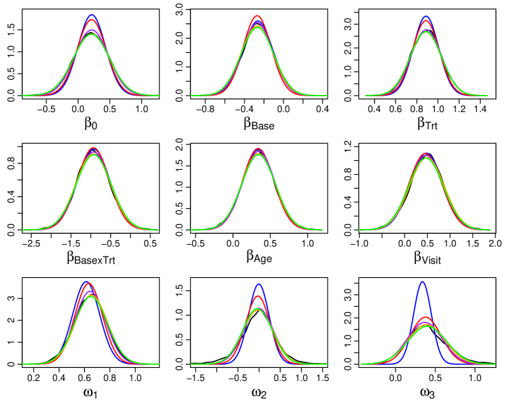
8.1 Epilepsy data
In this epilepsy data (Thall and Vail, 1990), patients are involved in a clinical trial to investigate the effects of the anti-epileptic drug Progabide. The patients are randomly assigned to receive either the drug (Trt = 1) or a placebo (Trt = 0). The response denotes the number of epileptic attacks patient had during 4 follow-up periods of two weeks each. Covariates include the log of the age of the patients (Age), the log of 1/4 the baseline seizure count recorded over an eight-week period prior to the trial (Base) and Visit (coded as Visit, Visit, Visit and Visit). Note that Age is centered about its mean. Consider , where
for (Breslow and Clayton, 1993).
Table 1 shows the results obtained from applying the variational algorithms to this data. The lower bounds are estimated using 1000 simulations in each case and the mean and standard deviation from these simulations are reported. CSGVA produced an improvement in the estimate of the lower bound (3139.2) as compared to GVA (3138.3) and maximizing the IWLB led to further improvements. Using a larger of 20 or 100 resulted in minimal improvements compared with . As this dataset is small, parallel computing is slower than serial for a small . This is because, even though the importance weights and gradients for samples are computed in parallel, the cost of sending and fetching data from the workers at each iteration dwarfs the cost of computation when is small. For , parallel computing reduces the computation time by about half.
| time | parallel | ||||
|---|---|---|---|---|---|
| GVA | 1 | 31 | 13.9 | - | 3138.3 (1.8) |
| CSGVA | 1 | 39 | 16.2 | - | 3139.2 (1.5) |
| IW-CSGVA | 5 | 1 | 2.5 | 6.1 | 3139.9 (0.7) |
| 20 | 1 | 6.9 | 8.1 | 3140.1 (0.4) | |
| 100 | 1 | 33.5 | 16.0 | 3140.1 (0.3) |
The estimated marginal posterior distributions of the global parameters are shown in Figure 1. The plots show that CSGVA (red) produces improved estimates of the posterior distribution as compared to GVA (blue), especially in estimating the posterior variance of the precision parameters and . The posteriors estimated using IW-CSGVA for the different values of are very close. By using just , we are able to obtain estimates that are virtually indistinguishable from that of MCMC.
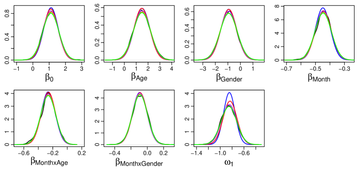
8.2 Madras data
These data come from the Madras longitudinal schizophrenia study (Diggle et al., 2002) for detecting a psychiatric symptom called “thought disorder”. Monthly records showing whether the symptom is present in a patient are kept for patients over 12 months. The response is a binary indicator for presence of the symptom. Covariates include the time in months since initial hospitalization (), gender of patient (Gender = 0 if male and 1 if female) and age of patient (Age = 0 if the patient is younger than 20 years and 1 otherwise). Consider and
for .
The results in Table 2 are quite similar to that of the epilepsy data. CSGVA yields an improvement in the lower bound estimate as compared to GVA and IW-CSGVA provided further improvements, which are evident starting with a as small as 5. Parallel computing halved the computation time for but did not yield any benefits for . From Figure 2, CSGVA and IW-CSGVA are again able to capture the posterior variance of the precision parameter better than GVA.
| time | parallel | ||||
|---|---|---|---|---|---|
| GVA | 1 | 25 | 13.1 | - | -383.4 (1.4) |
| CSGVA | 1 | 35 | 12.6 | - | -383.1 (1.4) |
| IW-CSGVA | 5 | 1 | 2.4 | 7.1 | -382.5 (0.7) |
| 20 | 1 | 6.8 | 8.9 | -382.4 (0.4) | |
| 100 | 1 | 33.9 | 16.8 | -382.3 (0.2) |
8.3 Six cities data
In the six cities data (Fitzmaurice and Laird, 1993), children from Steubenville, Ohio, are involved in a longitudinal study to investigate the health effects of air pollution. Each child is examined yearly from age 7 to 10 and the response is a binary indicator for wheezing. There are two covariates, (a binary indicator for smoking status of the mother of child ) and (age of child at time point , centered at 9 years). Consider , where
for .
| time | parallel | ||||
|---|---|---|---|---|---|
| GVA | 1 | 26 | 60.3 | - | -816.4 (4.0) |
| CSGVA | 1 | 28 | 36.5 | - | -816.0 (3.9) |
| IW-CSGVA | 5 | 1 | 6.5 | 16.3 | -812.6 (2.5) |
| 20 | 1 | 23.1 | 24.5 | -811.0 (1.9) | |
| 100 | 1 | 115.5 | 61.4 | -809.8 (1.5) |
From Table 3, CSGVA managed to achieve a higher lower bound than GVA in about half the runtime. As increases, IW-CSGVA produced tighter lower bounds for the log marginal likelihood. As in the previous two examples, parallel computing is beneficial only when , cutting the runtime by about half. From Figure 3, there is slight overestimation of the posterior means of and by all the variational methods. However, CSGVA and IW-CSGVA are able to capture the posterior variance of these parameters much better than GVA especially for .

9 Application to state space models
Here we consider the stochastic volatility model (SVM) widely used for modeling financial time series. Let each observation for , be generated from a zero-mean Gaussian distribution where the error variance is stochastically evolving over time. The unobserved log volatility is modeled using an autoregressive process of order one with Gaussian disturbances:
where , and . Here, represents the mean-corrected return at time and the states come from a stationary process with drawn from the stationary distribution. The parametrization of the SVM above is noncentered. The centered parametrization can be obtained by replacing by . The performance of GVA and CSGVA are sensitive to the parametrization both in terms of rate of convergence and attained local mode. For the data sets below, the noncentered parametrization was found to have better convergence properties. The sensitivity of the stochastic volatility model to parametrization when fitted using MCMC algorithms is well known in the literature. To “combine the best of different worlds”, Kastner and Frühwirth-Schnatter (2014) introduce a strategy that samples parameters from the centered and noncentered parametrizations alternately. Tan (2017) studies optimal partially noncentered parametrizations for Gaussian state space models fitted using EM, MCMC or variational algorithms.
We use the following transformations to map constrained parameters to :
This transformation for works better than , which leads to erratic fluctuations in the lower bound and convergence issues more often. The global variables are of dimension and the local variables are of length . We assume normal priors for the global parameters, where , and , where . The joint density can be written as
The log joint density is
where , and is a constant independent of . The gradient is given in Appendix C. For this model, is conditionally independent of in the posterior if given . Thus, the sparsity structure imposed on and are
The number of nonzero elements in is . Setting and for all and all , where denotes the set of indices in which are fixed as zero, the number of variational parameters to be optimized are reduced from to for , and from to for .
9.1 GBP/USD exchange rate data
This data contain 946 observations of the exchange rates of the US Dollar (USD) against the British Pound (GBP), recorded daily from 1 October 1981, to 28 June 1985. This data are available from the “Garch” dataset in the R package Ecdat. The mean-corrected responses are computed from the exchange rates as
where .
For this data, CSGVA failed to achieve a higher lower bound when it was initialized using . Hence we initialize CSGVA using the fit from GVA instead, by using the association discussed in Section 5. With this informative starting point, CSGVA converged in 16000 iterations and managed to improve upon the GVA fit, attaining a higher lower bound. IW-CSGVA led to further improvements with increasing . As this dataset contains a large number of observations with correspondingly more variational parameters to be optimized, the computation is more intensive and parallel computing comes in very useful reducing the computation time by factors of 1.8, 2.9 and 4.2 for respectively.
| time | parallel | ||||
|---|---|---|---|---|---|
| GVA | 1 | 61 | 239.7 | - | -138.2 (1.3) |
| CSGVA | 1 | 16 | 58.6 | - | -137.8 (1.3) |
| IW-CSGVA | 5 | 1 | 18.3 | 10.2 | -137.4 (1.0) |
| 20 | 1 | 71.2 | 24.4 | -137.0 (0.5) | |
| 100 | 1 | 355.3 | 84.3 | -136.8 (0.4) |
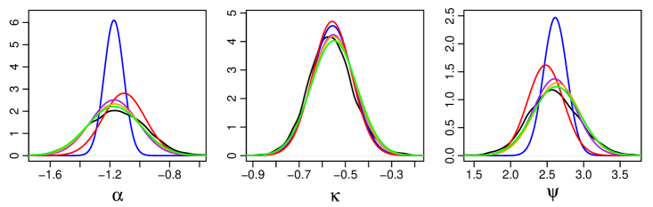
Figure 4 shows the estimated marginal posteriors of the global parameters. CSGVA provides significant improvements in estimating the posterior variance of and as compared to GVA. With the application of IW-CSGVA, we are able to obtain posterior estimates that are quite close to that of MCMC even with a small .
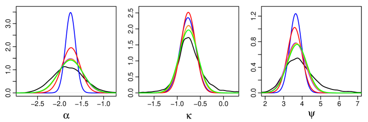
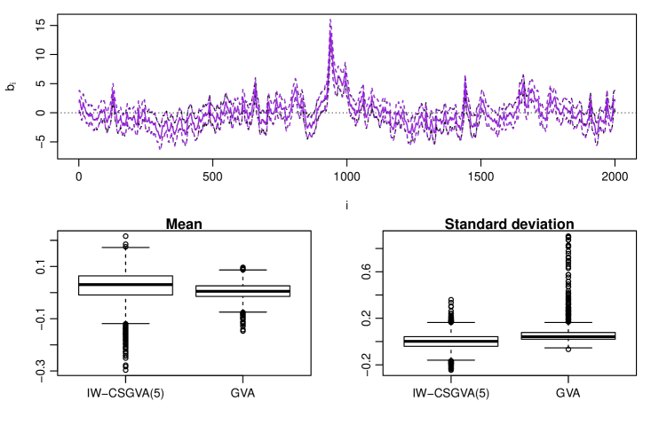
Figure 5 shows the estimated marginal posteriors of the latent states summarized using the mean (solid line) and one standard deviation from the mean (dotted line) estimated by MCMC (black) and IW-CSGVA (, purple).
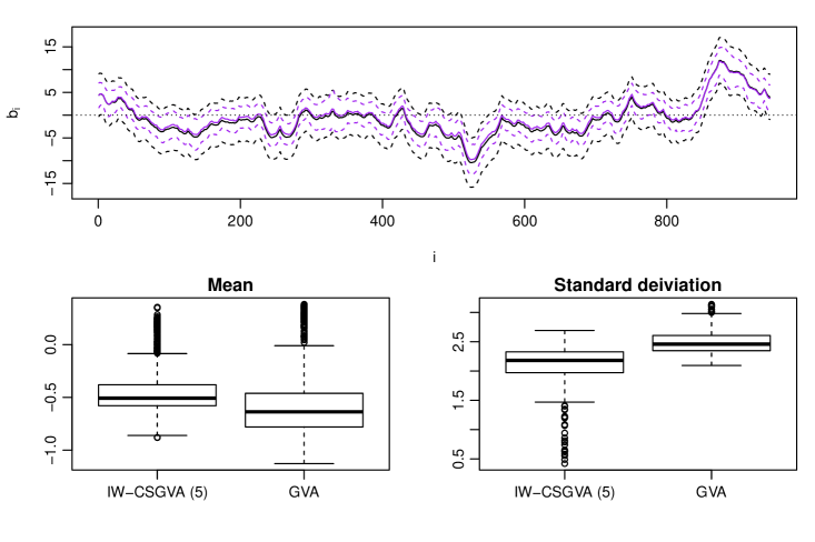
For IW-CSGVA, the means and standard deviations are estimated based on 2000 samples, by generating from followed by from . For MCMC, estimation was based on 5000 samples. IW-CSGVA estimated the means quite accurately (with a little overestimation) but the standard deviations are underestimated when compared to MCMC. The boxplots shows the difference between the means and standard deviations estimated by IW-CSGVA and GVA with MCMC. We can see that IW-CSGVA estimated both the means and standard deviations more accurately as compared to GVA.
9.2 New York stock exchange data
Next we consider 2000 observations of the returns of the New York Stock Exchange (NYSE) from February 2, 1984 to December 31, 1991. This data is available as the dataset “nyse” from the R package astsa. We consider 100 times the mean-corrected returns as responses .
From Table 5, CSGVA was able to attain a higher lower bound than GVA when initialized in the standard manner using . Applying IW-CSGVA led to further improvements as increases. For this massive data set, parallel computing yields significant reductions in computation time, by factors of 2.9, 4.5 and 5.5 corresponding to , 20, 100 respectively.
| time | parallel | ||||
|---|---|---|---|---|---|
| GVA | 1 | 43 | 679.0 | - | -570.8 (1.8) |
| CSGVA | 1 | 49 | 749.2 | - | -570.7 (2.0) |
| IW-CSGVA | 5 | 1 | 76.0 | 26.1 | -569.4 (1.1) |
| 20 | 1 | 305.0 | 67.9 | -569.0 (0.7) | |
| 100 | 1 | 1503.0 | 274.0 | -568.7 (0.4) |
Figure 6 shows that the marginal posteriors estimated using CSGVA are quite close to that of MCMC while GVA underestimated the posterior variance of and quite severely. Posteriors estimated by IW-CSGVA are virtually indistinguishable from MCMC.
From Figure 7, we can see that the marginal posteriors of the latent states are also estimated very well using IW-CSGVA and there is no systematic underestimation of the posterior variance unlike the previous example. GVA captures the posterior means very well but did not perform as well as IW-CSGVA in estimating the posterior variance.
10 Conclusion
In this article, we have proposed a Gaussian variational approximation for hierarchical models that adopts a conditional structure . The dependence of the local variables on global variables are then captured using a linear approximation. This structure is very useful when there are global scale parameters in which help to determine the scale of local variables in the conditional posterior of . We further demonstrate how CSGVA can be improved by maximizing the importance weighted lower bound. From our experiments, using a as small as 5 can lead to significant improvements in the variational approximation, with just a short run. Moreover, for massive datasets, computation time can be further reduced through parallel computing. Our experiments indicate that CSGVA coupled with importance weighting is particularly useful in improving the estimation of the posterior variance of precision parameters in GLMMs, and the persistence and volatility of the log-variance in SVMs.
References
- Archer et al. (2016) Archer E, Park IM, Buesing L, Cunningham J, Paninski L (2016) Black box variational inference for state space models. arXiv:1511.07367
- Blei et al. (2017) Blei DM, Kucukelbir A, McAuliffe JD (2017) Variational inference: A review for statisticians. Journal of the American Statistical Association 112:859–877
- Breslow and Clayton (1993) Breslow NE, Clayton DG (1993) Approximate inference in generalized linear mixed models. Journal of the American Statistical Association 88:9–25
- Burda et al. (2016) Burda Y, Grosse R, Salakhutdinov R (2016) Importance weighted autoencoders. In: Proceedings of the 4th International Conference on Learning Representations (ICLR)
- Diggle et al. (2002) Diggle PJ, Heagerty P, Liang KY, Zeger SL (2002) The analysis of Longitudinal Data, 2nd edn. Oxford University Press, Oxford
- Dinh et al. (2017) Dinh L, Sohl-Dickstein J, Bengio S (2017) Density estimation using real NVP. In: Proceedings of the 5th International Conference on Learning Representations (ICLR)
- Domke and Sheldon (2018) Domke J, Sheldon DR (2018) Importance weighting and variational inference. In: Bengio S, Wallach H, Larochelle H, Grauman K, Cesa-Bianchi N, Garnett R (eds) Advances in Neural Information Processing Systems 31, Curran Associates, Inc., pp 4470–4479
- Fitzmaurice and Laird (1993) Fitzmaurice GM, Laird NM (1993) A likelihood-based method for analysing longitudinal binary responses. Biometrika 80:141–151
- Germain et al. (2015) Germain M, Gregor K, Murray I, Larochelle H (2015) MADE: Masked autoencoder for distribution estimation. In: Bach F, Blei D (eds) Proceedings of the 32nd International Conference on Machine Learning, PMLR, Lille, France, Proceedings of Machine Learning Research, vol 37, pp 881–889
- Guo et al. (2016) Guo F, Wang X, Broderick T, Dunson DB (2016) Boosting variational inference. arXiv: 1611.05559
- Han et al. (2016) Han S, Liao X, Dunson DB, Carin LC (2016) Variational Gaussian copula inference. In: Gretton A, Robert CC (eds) Proceedings of the 19th International Conference on Artificial Intelligence and Statistics, JMLR Workshop and Conference Proceedings, vol 51, pp 829–838
- Hoffman and Blei (2015) Hoffman M, Blei D (2015) Stochastic structured variational inference. In: Lebanon G, Vishwanathan S (eds) Proceedings of the Eighteenth International Conference on Artificial Intelligence and Statistics, JMLR Workshop and Conference Proceedings, vol 38, pp 361–369
- Huszár (2017) Huszár F (2017) Variational inference using implicit distributions. arXiv:1702.08235
- Jaakkola and Jordan (1998) Jaakkola TS, Jordan MI (1998) Improving the mean field approximation via the use of mixture distributions, Springer Netherlands, Dordrecht, pp 163–173
- Kastner and Frühwirth-Schnatter (2014) Kastner G, Frühwirth-Schnatter S (2014) Ancillarity-sufficiency interweaving strategy (ASIS) for boosting MCMC estimation of stochastic volatility models. Computational Statistics and Data Analysis 76:408 – 423
- Kingma and Ba (2015) Kingma DP, Ba J (2015) Adam: A method for stochastic optimization. In: Proceedings of the 3rd International Conference on Learning Representations (ICLR)
- Kingma and Welling (2014) Kingma DP, Welling M (2014) Auto-encoding variational Bayes. In: Proceedings of the 2nd International Conference on Learning Representations (ICLR)
- Kingma et al. (2016) Kingma DP, Salimans T, Jozefowicz R, Chen X, Sutskever I, Welling M (2016) Improved variational inference with inverse autoregressive flow. In: Lee DD, Sugiyama M, Luxburg UV, Guyon I, Garnett R (eds) Advances in Neural Information Processing Systems 29, Curran Associates, Inc., pp 4743–4751
- Li and Turner (2016) Li Y, Turner RE (2016) Rényi divergence variational inference. In: Proceedings of the 30th International Conference on Neural Information Processing Systems, Curran Associates Inc., USA, NIPS’16, pp 1081–1089
- Maddison et al. (2017) Maddison CJ, Lawson J, Tucker G, Heess N, Norouzi M, Mnih A, Doucet A, Teh Y (2017) Filtering variational objectives. In: Guyon I, Luxburg UV, Bengio S, Wallach H, Fergus R, Vishwanathan S, Garnett R (eds) Advances in Neural Information Processing Systems 30, Curran Associates, Inc., pp 6573–6583
- Magnus and Neudecker (1980) Magnus JR, Neudecker H (1980) The elimination matrix: Some lemmas and applications. SIAM Journal on Algebraic Discrete Methods 1:422–449
- Magnus and Neudecker (1999) Magnus JR, Neudecker H (1999) Matrix differential calculus with applications in statistics and econometrics, 3rd edn. John Wiley & Sons, New York
- Miller et al. (2016) Miller AC, Foti N, Adams RP (2016) Variational boosting: Iteratively refining posterior approximations. arXiv: 1611.06585
- Minka (2005) Minka T (2005) Divergence measures and message passing. Tech. rep.
- Ormerod and Wand (2010) Ormerod JT, Wand MP (2010) Explaining variational approximations. The American Statistician 64:140–153
- Papaspiliopoulos et al. (2003) Papaspiliopoulos O, Roberts GO, Sköld M (2003) Non-centered parameterisations for hierarchical models and data augmentation. In: Bernardo JM, Bayarri MJ, Berger JO, Dawid AP, Heckerman D, Smith AFM, West M (eds) Bayesian Statistics 7, Oxford University Press, New York, pp 307–326
- Papaspiliopoulos et al. (2007) Papaspiliopoulos O, Roberts GO, Sköld M (2007) A general framework for the parametrization of hierarchical models. Statist Sci 22:59–73
- Ranganath et al. (2016) Ranganath R, Tran D, Blei DM (2016) Hierarchical variational models. In: Balcan MF, Weinberger KQ (eds) Proceedings of The 33rd International Conference on Machine Learning, JMLR Workshop and Conference Proceedings, vol 37, pp 324–333
- Regli and Silva (2018) Regli JB, Silva R (2018) Alpha-Beta divergence for variational inference. arXiv: 1805.01045
- Rényi (1961) Rényi A (1961) On measures of entropy and information. In: Proceedings of the Fourth Berkeley Symposium on Mathematical Statistics and Probability, Volume 1: Contributions to the Theory of Statistics, University of California Press, Berkeley, Calif., pp 547–561
- Rezende and Mohamed (2015) Rezende DJ, Mohamed S (2015) Variational inference with normalizing flows. In: Bach F, Blei D (eds) Proceedings of The 32nd International Conference on Machine Learning, JMLR Workshop and Conference Proceedings, vol 37, pp 1530–1538
- Rezende et al. (2014) Rezende DJ, Mohamed S, Wierstra D (2014) Stochastic backpropagation and approximate inference in deep generative models. In: Xing EP, Jebara T (eds) Proceedings of The 31st International Conference on Machine Learning, JMLR Workshop and Conference Proceedings, vol 32, pp 1278–1286
- Roeder et al. (2017) Roeder G, Wu Y, Duvenaud DK (2017) Sticking the landing: Simple, lower-variance gradient estimators for variational inference. In: Guyon I, Luxburg U, Bengio S, Wallach H, Fergus R, Vishwanathan S, Garnett R (eds) Advances in Neural Information Processing Systems 30
- Rothman et al. (2010) Rothman AJ, Levina E, Zhu J (2010) A new approach to Cholesky-based covariance regularization in high dimensions. Biometrika 97:539–550
- Salimans and Knowles (2013) Salimans T, Knowles DA (2013) Fixed-form variational posterior approximation through stochastic linear regression. Bayesian Analysis 8:837–882
- Smith et al. (2019) Smith MS, Loaiza-Maya R, Nott DJ (2019) High-dimensional copula variational approximation through transformation. arXiv:1904.07495
- Spall (2003) Spall JC (2003) Introduction to stochastic search and optimization: estimation, simulation and control. Wiley, New Jersey
- Spantini et al. (2018) Spantini A, Bigoni D, Marzouk Y (2018) Inference via low-dimensional couplings. Journal of Machine Learning Research 19:1–71
- Tan (2017) Tan LSL (2017) Efficient data augmentation techniques for gaussian state space models. arXiv:1712.08887
- Tan (2018) Tan LSL (2018) Use of model reparametrization to improve variational Bayes. arXiv:1805.07267
- Tan and Nott (2013) Tan LSL, Nott DJ (2013) Variational inference for generalized linear mixed models using partially non-centered parametrizations. Statistical Science 28:168–188
- Tan and Nott (2018) Tan LSL, Nott DJ (2018) Gaussian variational approximation with sparse precision matrices. Statistics and Computing 28:259–275
- Thall and Vail (1990) Thall PF, Vail SC (1990) Some covariance models for longitudinal count data with overdispersion. Biometrics 46:657–671
- Titsias and Lázaro-Gredilla (2014) Titsias M, Lázaro-Gredilla M (2014) Doubly stochastic variational Bayes for non-conjugate inference. In: Proceedings of the 31st International Conference on Machine Learning (ICML-14), pp 1971–1979
- Tran et al. (2015) Tran D, Blei DM, Airoldi EM (2015) Copula variational inference. In: Advances in Neural Information Processing Systems 28: Annual Conference on Neural Information Processing Systems 2015, December 7-12, 2015, Montreal, Quebec, Canada, pp 3564–3572
- Tucker et al. (2018) Tucker G, Lawson D, Gu S, Maddison CJ (2018) Doubly reparametrized gradient estimators for Monte Carlo objectives. arXiv: 1810.04152
- van Erven and Harremos (2014) van Erven T, Harremos P (2014) Rényi divergence and kullback-leibler divergence. IEEE Transactions on Information Theory 60:3797–3820
- Yang et al. (2019) Yang Y, Pati D, Bhattacharya A (2019) -variational inference with statistical guarantees. Annals of Statistics To appear
Appendix A Derivation of stochastic gradient
We have
where . Differentiating with respect to , is given by
Since does not depend on , , and , we have
It is easy to see that and . The rest of the terms are derived as follows.
Differentiating with respect to ,
Differentiating with respect to ,
Differentiating with respect to ,
Differentiating with respect to ,
Differentiating with respect to ,
Differentiating with respect to ,
Since and , we have
As and , differentiating with respect to ,
Therefore
Note that as is upper triangular and only retains the diagonal elements of .
Differentiating with respect to ,
Appendix B Gradients for generalized linear mixed models
Since , we require
For the centered parametrization, the components in are given below. Note that .
Differentiating with respect to ,
where and . Hence
Note that because is upper triangular and only retains the diagonal elements.
Appendix C Gradients for state space models
Since , we require
The components in are given below.
For ,