Confidence-Weighted Boundary-Aware Learning for Semi-Supervised Semantic Segmentation
Abstract
Semi-supervised semantic segmentation (SSSS) aims to improve segmentation performance by utilising unlabeled data alongside limited labeled samples. Existing SSSS methods often face challenges such as coupling, where over-reliance on initial labeled data leads to suboptimal learning; confirmation bias, where incorrect predictions reinforce themselves repeatedly; and boundary blur caused by insufficient boundary-awareness and ambiguous edge information. To address these issues, we propose CW-BASS, a novel framework for SSSS. In order to mitigate the impact of incorrect predictions, we assign confidence weights to pseudo-labels. Additionally, we leverage boundary-delineation techniques, which, despite being extensively explored in weakly-supervised semantic segmentation (WSSS) remain under-explored in SSSS. Specifically, our approach: (1) reduces coupling through a confidence-weighted loss function that adjusts the influence of pseudo-labels based on their predicted confidence scores, (2) mitigates confirmation bias with a dynamic thresholding mechanism that learns to filter out pseudo-labels based on model performance, (3) resolves boundary blur with a boundary-aware module that enhances segmentation accuracy near object boundaries, and (4) reduces label noise with a confidence decay strategy that progressively refines pseudo-labels during training. Extensive experiments on the Pascal VOC 2012 and Cityscapes demonstrate that our method achieves state-of-the-art performance. Moreover, using only 1/8 or 12.5% of labeled data, our method achieves a mIoU of 75.81 on Pascal VOC 2012, highlighting its effectiveness in limited-label settings.
Index Terms:
Semi-supervised Learning, Semantic Segmentation, Pseudo-Labeling, Confidence Weighting.I Introduction
Semantic segmentation, the task of assigning semantic labels to each pixel in an image, is fundamental to applications like autonomous driving, medical imaging, and scene understanding [10]. However, its success heavily relies on large-scale annotated datasets, which are expensive and labour-intensive to produce [2], creating significant challenges for adapting models to new datasets with limited labeled data [1]. To address this issue, researchers have increasingly focused on semi-supervised semantic segmentation (SSSS), which uses both labeled and unlabeled data through methods such as self-training (ie. pseudo-labeling) [14], consistency-based regularization [13], and generative models [22] to improve model generalisation and address the limitations of fully supervised techniques.
Early semi-supervised methods primarily used self-training due to its simplicity and effectiveness. In self-training, a teacher model is trained on a small set of labeled data to generate pseudo-labels for a larger set of unlabeled data. These pseudo-labels are later used to retrain the student model, effectively expanding the training dataset [3]. This approach has the ability to use large amounts of unlabeled data to learn more generalized features and improve the model’s robustness against overfitting and has proven especially useful in data-scarce domains like medical imaging [20]. Building on self-training, more sophisticated methods such as consistency, regularization, and generative models [22] [42] have been proposed. Consistency-based methods ensure that the model predictions remain stable under various input data perturbations, such as spatial transformations or intensity variations, promoting greater generalizations [22] [40]. Furthermore, generative models, such as Generative Adversarial Networks (GANs), have been used to synthesize training data or improve the quality of pseudo-labels derived from unlabeled data, thereby increasing the effectiveness of semi-supervised semantic segmentation [11].
Despite these advancements, issues such as coupling, confirmation bias and boundary delineation still persist due to label noise and limited labeled data [4]. The coupling problem occurs when the model’s predictions on unlabeled data are overly reliant on the initial labeled dataset, resulting in performance that is strongly correlated with the quality of the pseudo-labels generated. Previous studies have addressed this issue by proposing the use of exponential moving averages [5] and consistency regularisation [6]. However, these strategies frequently rely on fixed confidence levels that do not adapt to the model’s learning dynamics over time. This inflexibility can result in the premature exclusion of valuable low-confidence samples, reducing training diversity, and limiting generalization. Confirmation bias complicates this scenario by causing models to favour predictions that align with their initial biases, creating a feedback loop where errors in pseudo-labels are repeatedly reinforced, ultimately degrading model performance. In [29], the authors demonstrate that generating pseudo-labels under significant intra-class variation frequently results in poor representation of the data distribution, reducing generalisation.
Boundary blur occurs when a model fails to accurately recognize the correct category of pixels at object boundaries, reducing segmentation performance. This problem is most common in weakly-supervised semantic segmentation (WSSS), where boundary-delineating methods have been proposed to reduce the effects of inaccurate pixel-level annotations [29] [41]. However, despite the extensive research of these techniques in WSSS, their application in semi-supervised semantic segmentation (SSSS) remains relatively under-explored, highlighting a critical gap in the current research landscape [32].
To tackle these limitations, we propose a novel dual-stage training framework that integrates dynamic confidence and boundary-delineation methods. We specifically solve the aforementioned issues and achieve good segmentation performance as demonstrated in Fig. 1. Our approach achieves good segmentation performance compared to SOTA methods, ST++ [9] and UniMatch [36] on the Pascal VOC dataset.
Our key contributions are summarised as follows:
-
1.
Confidence-Weighted Loss Function: We apply a novel confidence-weighted cross-entropy loss function that adjusts pixel contribution to the total loss based on confidence score, enabling more reliable predictions while learning from less certain ones.
-
2.
Dynamic Thresholding Mechanism: We introduce an adaptive thresholding mechanism that updates the pseudo-label confidence threshold according to the model’s training performance, ensuring accurate predictions without discarding potentially valuable low-confidence data.
-
3.
Boundary Aware Technique: We introduce a boundary-aware technique module to enhance the model’s ability to learn intricate, fine-grained details, significantly improving segmentation accuracy, especially near object boundaries.
-
4.
Confidence Decay Strategy: We employ a confidence decay strategy that progressively reduces the influence of low-confidence pseudo-labels during training, promoting exploration early on and focusing on high-confidence predictions as the model stabilizes.
II Related Work
II-A Pseudo-Labeling
Pseudo-labeling is an important method in semi-supervised learning (SSL), where model predictions on unlabeled data become pseudo-labels for subsequent training [14]. Pseudo-labeling, although effective, is vulnerable to error propagation, whereby inaccurate pseudo-labels aggravate model biases and reduce performance [15]. Consequently, teacher-student frameworks attempt to solve this issue by enhancing the stability of pseudo-labeling through the use of an exponential moving average (EMA) of the students’ weights [16]. Advanced self-training methods such as ST++ [9] refine the teacher model iteratively using pseudo-labels generated by the student model. Likewise, PrevMatch [10] reconsiders predictions from earlier teacher models to produce more dependable pseudo-labels and address confirmation bias.
In this work, we extend these approaches by introducing a dynamic thresholding mechanism that adjusts to the model’s evolving confidence levels during training. Unlike prior methods such as [9] and [10] which employ static thresholds, our adaptive thresholding enhances label reliability by filtering out low-confidence predictions as the model learns. Additionally, we implement a confidence decay strategy that progressively reduces the influence of noisy pseudo-labels, further mitigating the impact of incorrect predictions.
II-B Consistency Regularization
Several studies rely on consistency regularization where model predictions remain stable despite input perturbations. Previous methods, including Temporal Ensembling [13] and Virtual Adversarial Training (VAT) [12] proved consistency by comparing predictions made on different versions of the same data. [8] improved the aforementioned method with teacher-based VAT (T-VAT), which uses adversarial perturbations within a teacher-student framework to create complex pseudo-labels, enhancing the generalization of the student model. Similarly, in [11], the author uses an adaptive ramp-up method to leverage two student networks that provide interactive feedback to the teacher model, enhancing pseudo-label quality and training consistency.
II-C Boundary Refined Semantic Segmentation
Techniques such as boundary refinement modules and edge detection have been used to enhance the accuracy of object edges in weakly-supervised semantic segmentation (WSSS). For example, Class Activation Mapping (CAM) has been utilised to generate coarse localisation maps, yet it often fails to capture intricate boundary details, resulting in suboptimal segmentation results [29] [32]. On the other hand, in semi-supervised semantic segmentation (SSSS), boundary-aware methods remain underexplored. [34] proposed refining boundary delineation by dynamically generating and optimizing class prototypes near boundaries using high- and low-confidence feature clustering. Our novel approach uses Sobel filters to detect edges and create a binary boundary mask, which produces a boundary-aware loss to enhance the model’s focus on fine-grained details while improving segmentation accuracy near object boundaries.
III Method
Our proposed method, Confidence-Weighted Boundary-Aware Learning (CW-BASS) operates in two stages as shown in Fig. 2. In the first stage, the teacher model generates pseudo-labels with confidence scores for unlabeled data, which are used to calculate a confidence-weighted loss. Dynamic thresholding adjusts the confidence threshold adaptively, filtering low-confidence pseudo-labels based on training performance. In the second stage, a confidence decay strategy reduces the influence of low-confidence pixels, and a boundary-aware module enhances segmentation accuracy near object boundaries. The student model is ultimately trained using the final loss to produce segmentation results and the teacher model is updated.
III-A Stage 1: Training the Teacher Model
III-A1 Pseudo-Label Generation with Confidence Estimation
We address the problem of semantic segmentation in a semi-supervised setting, where a labeled dataset and an unlabeled dataset are available, with and representing the number of samples in the labeled and unlabeled datasets, respectively.
We train a teacher model on , and use it to generate high-quality pseudo-labels for and train a student model that improves performance on both datasets.
For each unlabeled image , the teacher model, generates logits, :
| (1) |
From these logits, we derive pseudo-labels, and pixel-wise confidence scores, :
| (2) |
| (3) |
where is the pseudo-label for pixel in image ;
represents the confidence score for pixel ; and
is the index of the possible classes.
III-A2 Confidence-Weighted Loss
The loss consists of labeled and unlabeled components:
Confidence-Weighted Cross-Entropy Loss. To address the label noise introduced by inaccurate pseudo-labels from the teacher, we propose a confidence-weighted loss that weights the contribution of each pixel to the overall loss based on its confidence score. The pixel-wise confidence is raised to a power to emphasize high-confidence predictions:
The loss for an unlabeled image, is defined as:
| (4) |
where is the total number of pixels in image ;
are the logits predicted by the student model ; and
is the hyperparameter controlling emphasis on high-confidence predictions.
Loss for Labeled Data. For labeled data, we use the standard cross-entropy loss:
| (5) |
where is the ground truth label for pixel in image .
Total Loss. The total loss is a combination of the losses from labeled and unlabeled data:
| (6) |
where is a balancing parameter between the supervised and unsupervised losses.
III-A3 Dynamic Thresholding Mechanism
We introduce a dynamic threshold mechanism to adaptively learn and adjust the confidence threshold for filtering low-confidence pseudo-labels, based on the model’s performance during training.
Average Confidence Calculation. For each batch, we calculate the average confidence score :
| (7) |
where is the average confidence.
Dynamic Threshold Adjustment. The base threshold is then adjusted using a logistic function based on the average confidence:
| (8) |
where is the initial confidence threshold, is the initial average confidence and is a hyperparameter controlling the sensitivity of the threshold adjustment.
Retaining Pseudo-labels. We retain pseudo-labels where the confidence score exceeds the threshold:
| (9) |
III-B Stage 2: Training the Student Model
III-B1 Confidence Decay Strategy
To further reduce the influence of consistently low-confidence pixels, we introduce a confidence decay strategy that progressively reduces the influence of low-confidence pseudo-labels over time:
For low-confidence pixels, we update their confidence scores as:
| (10) |
where is the confidence score at epoch and is the decay factor.
III-B2 Boundary-Aware Learning
After the pseudo-labels are refined and filtered through confidence weighting and thresholding, we introduce boundary-aware learning to focus on the more intricate task of boundary delineation and overall improve segmentation performance.
Boundary Detection. We apply Sobel filters to the pseudo-labels to detect edges [30]. Let and be the horizontal and vertical gradients, respectively. The gradient magnitude at pixel, in image, is:
| (11) |
A binary boundary mask is then defined as:
| (12) |
where is the gradient magnitude at pixel ; are the pixel gradients at derived via Sobel filters and is the binary mask indicating boundaries (if , else ).
Boundary-Aware Loss. To emphasize correct predictions at boundaries, we scale the cross-entropy loss by the boundary mask to encourage the model to focus more on object contours:
| (13) |
where is the pixel-wise cross-entropy at pixel and is the total number of pixels in image .
III-B3 Final Combined Loss
The final loss function combines all components:
| (14) |
III-B4 Model Update
Student Model. The student model is trained using and the refined pseudo-labeled data :
| (15) |
Teacher Model. Once is trained, we set:
| (16) |
IV Experiments
IV-A Dataset
For semi-supervised settings, we evaluate our method under various labeled data partitions, such as , , , and of the full labeled dataset. We perform experiments on two benchmark datasets: Pascal VOC 2012 [23] and Cityscapes [24] with comparisons with state-of-the-art methods.
IV-A1 Pascal VOC 2012
This dataset consists of 1,464 training images and 1,449 validation images, annotated with 21 semantic classes including the background.
IV-A2 Cityscapes
Cityscapes contains 2,975 training images and 500 validation images, with high-resolution street scenes annotated into 19 classes.
IV-B Setup
IV-B1 Network Architecture
IV-B2 Training Setup
For optimization, we employ stochastic gradient descent (SGD) with a momentum of 0.9 and a weight decay of . The learning rate (LR) and scheduler are as follows: Pascal VOC: 0.001, and for Cityscapes: 0.004 due to larger image sizes and batch adjustments.
A polynomial learning rate decay is used, defined as: .
Batch size for Pascal VOC is set to 16, and for Cityscapes, due to higher resolution, is set to 8. The model is trained for 80 epochs on Pascal and 240 epochs on Cityscapes. It is also important to note, for fair comparisons with existing methods and to reduce computational costs, that our method does not use advanced optimization strategies such as OHEM, auxiliary supervision [18], or SyncBN, which are commonly used in other studies.
| Method | Pascal VOC 2012 | Cityscapes | ||||||
|---|---|---|---|---|---|---|---|---|
| 1/16 (92) | 1/8 (183) | 1/4 (366) | 1/2 (732) | 1/30 (100) | 1/16 (186) | 1/8 (372) | 1/4 (744) | |
| SupOnly* | 44.00 | 52.30 | 61.70 | 66.70 | 55.10 | 63.30 | 70.20 | 73.12 |
| ST [9] | 71.60 | 73.30 | 75.00 | - | 60.90 | - | 71.60 | 73.40 |
| ST++ [9] | 72.60 | 74.40 | 75.40 | - | 61.40 | - | 72.70 | 73.80 |
| MT [16] | 66.77 | 70.78 | 73.22 | 74.75 | - | 66.14 | 72.03 | 74.47 |
| GCT [17] | 64.05 | 70.47 | 73.45 | 75.20 | - | 65.81 | 71.33 | 75.30 |
| CPS [18] | 71.98 | 73.67 | 74.90 | 76.15 | - | 74.47 | 76.61 | 77.83 |
| ELN [19] | - | 73.30 | 74.63 | - | - | - | 70.33 | 73.52 |
| ESL [37] | 61.74 | 69.50 | 72.63 | 74.69 | - | 71.07 | 76.25 | 77.58 |
| PS-MT [20] | 72.80 | 75.70 | 76.02 | 76.64 | - | 74.37 | 76.92 | 77.64 |
| UniMatch [36] | 71.90 | 72.48 | 75.96 | 77.09 | - | 74.03 | 76.77 | 77.49 |
| CPSR [21] | 72.20 | 73.02 | 76.00 | 77.31 | - | 74.49 | 77.25 | 78.01 |
| CW-BASS (Ours) | 72.80 | 75.81 | 76.20 | 77.15 | 65.87 | 75.00 | 77.20 | 78.43 |
IV-B3 Implementation Details
We apply similar semi-supervised training settings as most state-of-the-art-methods to ensure fair comparisons. Data augmentation techniques include random horizontal flipping and random scaling (ranging from 0.5 to 2.0) [9]. We use reduced cropping sizes during training compared to CPS [18], ie. 321 × 321 pixels on Pascal VOC and 721 × 721 pixels on Cityscapes to save memory. On unlabeled images, we also utilize color jitter with the same intensity as [25], grayscale conversion, Gaussian blur as stated in [26], and Cutout with randomly filled values. All unlabeled images undergo test-time augmentation as well [18].
IV-B4 Evaluation Metrics
We use the standard mean Intersection over Union (mIoU) metric to evaluate segmentation performance. No ensemble techniques where used for all evaluations.
IV-B5 Hyperparameters
In our experiments, we use specific hyperparameters with default settings, and their impact is further analyzed in the ablation studies. Confidence Weighting () is set to a default value of 1.0, to balance the contribution of high- and low-confidence pseudo-labels in the confidence-weighted loss. For Dynamic Thresholding (), the base threshold () is 0.6, allowing the model to learn filter pseudo-labels dynamically based on its performance, thereby mitigating confirmation bias. Additionally, a sensitivity parameter () with a default value of 0.5 ensures stability by preventing the thresholds from becoming excessively lenient or overly strict. Lastly, the Confidence Decay Factor () is set to 0.9, to gradually reduces the influence of low-confidence pseudo-labels over time and refine the learning process.
IV-C Quantitative Analysis
IV-C1 Comparison on Computational Costs and Training Flows
Figure 5 illustrates the convergence behavior and performance of CW-BASS compared to the self-training method ST++ [9] on the Cityscapes dataset during the initial 20 epochs, utilizing the 1/16 partition protocol. CW-BASS achieves faster stabilization due to its confidence-weighted loss, which prioritizes high-confidence predictions and mitigates the influence of noisy pseudo-labels. Furthermore, its boundary-aware learning enhances segmentation accuracy near object edges, contributing to more rapid convergence. In contrast, ST++ depends on iterative retraining after selecting reliable images post pseudo-labeling. Overall, CW-BASS integrates swift initial convergence with sustained performance improvements throughout the training process.
Table II summarises data utilisation and training overhead for various approaches, highlighting differences in the number of networks trained, unlabeled data processed per epoch, and total training epochs. CPS has a dual network design and treats the labeled set, without the ground truth as additional unlabeled set, increasing the volume of training data. On the other hand, PS-MT implements consistency learning with perturbations to both teacher and student networks. CPS trains two networks, processing 10.5k and 2.9k unlabeled images per epoch on Pascal VOC and Cityscapes, respectively. PS-MT employs three networks with aggressive augmentations, often doubling or tripling unlabeled data (e.g., 19.8k samples per epoch for the 1/16 Pascal partition) and requires 320–550 epochs on Cityscapes. ST++ trains four networks with slightly fewer unlabeled samples per epoch compared to PS-MT (14.8k on Pascal and 4.1k on Cityscapes, both below 1/16). In contrast, CW-BASS trains two networks with fewer augmentations, using the least unlabeled data (up to 9.9k on Pascal and 2.7k on Cityscapes) and converging in just 80 epochs on Pascal and 240 epochs on Cityscapes, regardless of partition. This balanced approach achieves competitive performance while avoiding the overheads of intensive augmentations or large network ensembles.
IV-C2 Comparison on Segmentation Performance
Our proposed CW-BASS framework achieves state-of-the-art segmentation performance on both Pascal VOC 2012 and Cityscapes, as shown in Table I.
Results on Pascal VOC. Table I compares performance on the Pascal VOC 2012 dataset using various state-of-the-art (SOTA) semi-supervised semantic segmentation methods. Unlike approaches that use multiple teacher networks and various perturbations, our method relies on a single model for self-training. To highlight our performance, we also specifically compare our results with ST++, an advanced and simple self-training approach.
Using only 1/8 (12.5%) of the labeled training data, our method produces a mean Intersection over Union (mIoU) of 75.81%, outperforming existing state-of-the-art approaches. This also exceeds the performance of the fully supervised baseline by a remarkable 11.2%, demonstrating the effectiveness of our semi-supervised learning method in limited label settings.
Results on Cityscapes. Our method also outperforms state-of-the-art methods on the Cityscapes dataset as shown in Table I. Cityscapes presents more complex, high-resolution urban environments. Under an extremely limited and rarely used setting, where only 1/30 (3.3%) of the training data (100 labeled images) is annotated, our method achieves a remarkable mIoU of 65.87%. This surpasses the supervised baseline by 10.77%, showcasing our model’s efficiency in extremely limited label scenarios and ability to handle complex scene layouts, fine-grained object boundaries, and diverse urban visuals.
IV-D Qualitative Analysis
Fig. 1 and Fig. 4 show visual segmentation outputs produced by our method, CW-BASS on Pascal VOC and Cityscapes dataset, compared against a prominent self-training state-of-the-art method, ST++ [9] and UniMatch [36]. The qualitative gains are shown, with our method consistently providing clearer object boundaries, more accurate region delineations, and better overall segmentation performance. These results reflect the quantitative findings, showing the robustness and versatility of the proposed framework.
IV-E Ablation Studies
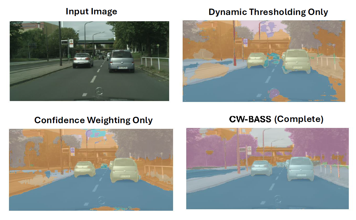
We conduct ablation studies on the various components of our CW-BASS framework to demonstrate their individual effectiveness. Table III shows the effectiveness of each component on the Pascal VOC dataset with a training size of 321 × 321 under a 1/8 (12.5%) labeled partition. Fig. 5 shows the visual comparisons of the predicted masks produced by each component on Cityscapes. We use the standard model (SupOnly) trained with only labeled images as our baseline.
IV-E1 Ablation Analysis
Confidence-Weighted Loss ( + ) Confidence-Weighting serves as the main component in our method () and () and achieves a mean Intersection over Union (mIoU) of 73.43%. This result is much higher than the baseline and some previous SOTA methods, underscoring the importance of the weighted loss in prioritizing high-confidence pseudo-labels and effectively mitigate the impact of label noise on model performance.
Boundary-Aware Loss (). Incorporating boundary-aware loss into the confidence-weighting, significantly improves segmentation performance, particularly near object boundaries. This addition results in an mIoU of 74.67%, marking a notable improvement of 6.36%. The findings demonstrate the effectiveness of addressing boundary blur through specialized loss functions.
Dynamic Thresholding Mechanism (). The integration of a dynamic thresholding mechanism enhances the model’s ability to filter out low-confidence pseudo-labels. Using this mechanism in conjunction with and yields an mIoU of 69.01%, highlighting its role in dynamically refining pseudo-label quality by discarding unreliable predictions.
Confidence Decay Strategy (). The confidence decay strategy gradually reduces the influence of low-confidence pseudo-labels during training. This approach stabilizes learning by improving pseudo-label reliability over time. The configuration () produces modest improvements, showcasing its ability to complement other strategies by enhancing pseudo-label robustness.
Discussion. The ablation study highlights the Confidence-Weighted Loss and Boundary-Aware Loss as the primary contributors to performance gains. The significant improvement observed with boundary-aware loss highlights the effectiveness of integrating boundary-delineation techniques in semi- supervised frameworks. The Confidence Decay Strategy and Dynamic Thresholding Mechanism address the challenges of noisy pseudo-labels and confirmation bias.
| mIoU(%) | |||||
|---|---|---|---|---|---|
| ✓ | ✓ | ✓ | 68.31 | ||
| ✓ | ✓ | ✓ | 69.01 | ||
| ✓ | ✓ | 73.43 | |||
| ✓ | ✓ | ✓ | 74.67 | ||
| ✓ | ✓ | ✓ | ✓ | ✓ | 75.81 |
| Hyperparameter group | Hyperparameter values | mIoU (%) |
|---|---|---|
| Standard Settings | 75.81 | |
| Conservative Settings | 71.40 |
IV-E2 Hyperparameter Analysis
To investigate the impact of our hyperparameter on model performance, we perform experiments using two groups of settings: our standard & default setting (i.e., ), which we use for all our experiments, and a more conservative setting (), as shown in Table IV. The standard settings batch yield the best model performance because the parameters are balanced, whereas the conservative settings yield an mIoU 4.41% lower than the standard settings.
For Confidence weighting, a value of 0.5 reduces the influence of these labels, making the model more conservative to minimize the risk of overfitting to incorrect labels. On the other hand, setting () to 2.0 increases the emphasis on high-confidence pseudo-labels, encouraging the model to reinforce confident predictions more aggressively.
Dynamic thresholding () involves a base threshold () set at 0.6, which is adjusted using a parameter . A higher value (e.g., 1.0) imposes stricter filtering, discarding more low-confidence pseudo-labels. To maintain stability, thresholds are constrained within a range of 0.3 to 0.8, ensuring they do not become excessively lenient or overly strict.
Finally, the confidence decay factor (), with a default value of 0.9, can be adjusted for specific training needs. Lowering to 0.85 accelerates the decay, which is particularly useful when a more aggressive reduction of noisy pseudo-labels is required.
V Conclusion
In this work, we presented Confidence-Weighted Boundary-Aware Semantic Segmentation (CW-BASS), a novel framework for semi-supervised semantic segmentation that addressed key challenges such as confirmation bias, boundary blur, and label noise. CW-BASS integrates confidence-weighting, dynamic thresholding, and boundary-delineation techniques to achieve state-of-the-art performance. CW-BASS significantly reduces the computational cost by using only two networks, fewer augmentations, and fewer unlabeled data samples per epoch, resulting in fewer training epochs while maintaining competitive performance. This efficient design is especially useful for resource-constrained scenarios because it balances performance and cost-effectiveness. Furthermore, CW-BASS’s fast initial convergence and robust boundary delineation make it suitable for real-world applications with limited computational resources and unlabeled data.
References
- [1] T.-H. Vu, H. Jain, M. Bucher, M. Cord, and P. Pérez, "ADVENT: Adversarial Entropy Minimization for Domain Adaptation in Semantic Segmentation," in Proceedings of the IEEE/CVF Conference on Computer Vision and Pattern Recognition (CVPR), pp. 2517–2526, 2019.
- [2] S. Li, C. Zhang, and X. He, "Shape-Aware Semi-Supervised 3D Semantic Segmentation for Medical Images," in Proceedings of Medical Image Computing and Computer-Assisted Intervention (MICCAI), pp. 552–561, 2020.
- [3] Z. Ke, D. Qiu, K. Li, Q. Yan, and R. W. H. Lau, "Guided Collaborative Training for Pixel-Wise Semi-Supervised Learning," in Proceedings of the European conference on computer vision (ECCV), pp. 429–445, 2020.
- [4] Y. Zou, Z. Yu, B. V. K. Kumar, and J. Wang, "Unsupervised Domain Adaptation for Semantic Segmentation via Class-Balanced Self-Training," in Proceedings of the European conference on computer vision (ECCV), pp. 289–305, 2018.
- [5] Y. Jiang, Y. Chen, Y. He, Q. Xu, Z. Yang, X. Cao, and Q. Huang, "MaxMatch: Semi-Supervised Learning With Worst-Case Consistency," IEEE Trans. Pattern Anal. Mach. Intell., vol. 45 no. 5, pp. 5970–5987, 2022.
- [6] S. Karlos, G. Kostopoulos, and S. Kotsiantis, "A Soft-Voting Ensemble Based Co-Training Scheme Using Static Selection for Binary Classification Problems," Algorithms, vol. 13, no. 26, pp. 1–19, 2020.
- [7] X. Shi, X. Xu, W. Zhang, X. Zhu, C. S. Foo, and K. Jia, "Open-Set Semi-Supervised Learning for 3D Point Cloud Understanding," arXiv preprint arXiv:2205.01006, 2022.
- [8] Y. Wang et al., "Semi-supervised semantic segmentation using unreliable pseudo-labels," in Proceedings of the IEEE/CVF Conference on Computer Vision and Pattern Recognition (CVPR), pp. 4248-4257, 2022.
- [9] L. Yang et al., "ST++: Make self-training work better for semi-supervised semantic segmentation," in Proceedings of the IEEE/CVF Conference on Computer Vision and Pattern Recognition (CVPR), pp. 4268–4277, 2022.
- [10] W. Shin et al., "Revisiting and maximizing temporal knowledge in semi-supervised semantic segmentation," arXiv preprint arXiv:2405.20610, 2024.
- [11] H. Cho et al., “Interactive Network Perturbation between Teacher and Students for Semi-Supervised Semantic Segmentation," in Proceedings of the IEEE/CVF Winter Conference on Applications of Computer Vision (WACV), pp. 626–635, 2024.
- [12] T. Miyato et al., "Virtual adversarial training: A regularization method for supervised and semi-supervised learning," IEEE Trans. Pattern Anal. Mach. Intell., vol. 41, no. 8, pp. 1979–1993, 2018.
- [13] S. Laine, T. Aila, "Temporal resembling for semi-supervised learning," arXiv preprint arXiv:1610.02242, 2016.
- [14] D. H. Lee, "Pseudo-Label: The Simple and Efficient Semi-Supervised Learning Method for Deep Neural Networks," in Proceedings of International Conference on Machine Learning (ICML) Workshop on Challenges in Representation Learning, pp. 896–901, 2013.
- [15] M. Zhang et al., "Semi-supervised bidirectional long short-term memory and conditional random fields model for named-entity recognition using embeddings from language models," Entropy, vol. 22, no. 2, pp. 1–19, 2020.
- [16] A. Tarvainen and H. Valpola, "Mean teachers are better role models: Weight-averaged consistency targets improve semi-supervised deep learning results," in Proceedings of Advances in Neural Information Processing Systems (NIPS), pp. 1195–-1204, 2017.
- [17] Z. Ke et al., "Guided collaborative training for pixel-wise semi-supervised learning," in Proceedings of the European Conference on Computer Vision (ECCV), pp. 429–445, 2020.
- [18] X. Chen et al., "Semisupervised semantic segmentation with cross pseudo supervision," in Proceedings of the IEEE/CVF Conference on Computer Vision and Pattern Recognition (CVPR), pp. 2613–2622, 2021.
- [19] D. Kwon and S. Kwak, "Semi-supervised semantic segmentation with error localization network," in Proceedings of the IEEE/CVF Conference on Computer Vision and Pattern Recognition (CVPR), pp. 9957–-9967, 2022.
- [20] Y. Liu et al., "Perturbed and strict mean teachers for semi-supervised semantic segmentation," in Proceedings of the IEEE/CVF Conference on Computer Vision and Pattern Recognition (CVPR), pp. 4258-–4267, 2022.
- [21] J. Yin, S. Yan, T. Chen, Y. Chen, and Y. Yao, “Class probability space regularization for semi-supervised semantic segmentation,” Comput. Vis. Image Underst., vol. 249, pp. 104146–104155, 2024.
- [22] Y. Zhang, Z. Gong, X. Zhao, X. Zheng, and W. Yao, "Semi supervised semantic segmentation with uncertainty-guided self cross supervision," in Proceedings of the Asian Conference on Computer Vision (ACCV), pp. 4631–-4647, 2022.
- [23] M. Everingham, L. Van Gool, C. K. I. Williams, J. Winn, and A. Zisserman, "The Pascal Visual Object Classes (VOC) Challenge," Int. J. Comput. Vis., vol. 88, no. 2, pp. 303–338, 2010.
- [24] M. Cordts, M. Omran, S. Ramos, T. Rehfeld, M. Enzweiler, R. Benenson, U. Franke, S. Roth, and B. Schiele, "The Cityscapes Dataset for Semantic Urban Scene Understanding," in Proceedings of the IEEE/CVF Conference on Computer Vision and Pattern Recognition (CVPR), pp. 3213–3223, 2016.
- [25] Y. Zou, Z. Zhang, H. Zhang, C.-L. Li, X. Bian, J.-B. Huang, and T. Pfister, "PseudoSeg: Designing Pseudo Labels for Semantic Segmentation," in arXiv preprint arXiv:2010.09713, 2020.
- [26] X. Chen, H. Fan, R. Girshick, and K. He, "Improved Baselines with Momentum Contrastive Learning," arXiv:2003.04297, 2020.
- [27] X. Chen, Y. Yuan, G. Zeng, and J. Wang, "Semi-supervised Semantic Segmentation with Cross Pseudo Supervision," in Proceedings of the IEEE/CVF Conference on Computer Vision and Pattern Recognition (CVPR), pp. 2613–2622, 2021.
- [28] H. Hu, F. Wei, H. Hu, Q. Ye, J. Cui, and L. Wang, "Semi-supervised Semantic Segmentation via Adaptive Equalization Learning," in Proceedings of Advances in Neural Information Processing Systems (NeurIPS), pp. 22106–22118, 2021.
- [29] S. Zheng, H. Wang, and X. Liu, “IntraMix: Intra-Class Mixup Generation for Accurate Labels and Neighbors,” arXiv preprint arXiv:2405.00957, 2024.
- [30] Jensen, P. M., Dahl, A. B., and Dahl, V. A. “Multi-object graph-based segmentation with non-overlapping surfaces,” In Proceedings of IEEE/CVF Conference on Computer Vision and Pattern Recognition Workshops (CVPRW), pp. 976–977, 2020.
- [31] Y. Zhang, B. Guo, Q. Dong, and Q. He, “Equilibrium and integrity correction class activation map in weakly supervised semantic segmentation,” In Proceedings of Fourth International Conference on Computer Vision and Data Mining (ICCVDM), vol. 108, pp. 13–24, 2023.
- [32] Z. Xu, Z. Xu, S. Zhang, and T. Lukasiewicz, “PCA: semi-supervised segmentation with patch confidence adversarial training,” arXiv preprint arXiv:2207.11683, 2022.
- [33] L. Zheng and D. Chen, “Weakly supervised and semi-supervised semantic segmentation for optic disc of fundus image,” Symmetry, vol. 12, no. 1, pp. 145-158, 2020.
- [34] J. Dong, Z. Meng, D. Liu, J. Liu, Z. Zhao, and F. Su, “Boundary-refined prototype generation: A general end-to-end paradigm for semi-supervised semantic segmentation,” Eng. Appl. Artif. Intell., vol. 137, pp. 109021–109040, 2024.
- [35] Z. Zhao, L. Yang, S. Long, J. Pi, L. Zhou, and J. Wang, “Augmentation matters: A simple-yet-effective approach to semi-supervised semantic segmentation,” in Proceedings of the IEEE/CVF Conference on Computer Vision and Pattern Recognition (CVPR), pp. 11350–11359, 2021.
- [36] L. Yang, L. Qi, L. Feng, W. Zhang, and Y. Shi, “Revisiting weak-to-strong consistency in semi-supervised semantic segmentation,” in Proceedings of the IEEE/CVF Conference on Computer Vision and Pattern Recognition (CVPR), pp. 7236–7246, 2023.
- [37] J. Ma, C. Wang, Y. Liu, L. Lin, and G. Li, “Enhanced soft label for semi-supervised semantic segmentation,” in Proceedings of the IEEE/CVF International Conference on Computer Vision (CVPR), pp. 1185–1195, 2023.
- [38] K. He, X. Zhang, S. Ren, and J. Sun. Deep residual learning for image recognition. In Proceedings of the IEEE Conference on Computer Vision and Pattern Recognition (CVPR), pp. 770–778, 2016.
- [39] J. Deng, W. Dong, R. Socher, L. Li, K. Li, and L. Fei-Fei. Imagenet: A large-scale hierarchical image database. In Proceedings of the IEEE Conference on Computer Vision and Pattern Recognition (CVPR), pp. 248–255, 2009.
- [40] B. W. Hwang, S. Kim, and S. W. Lee, A full-body gesture database for automatic gesture recognition, in Proceedings of the 7th International Conference on Automatic Face and Gesture Recognition, pp. 243–248, 2006.
- [41] M. S. Lee, Y. M. Yang, and S. W. Lee, Automatic video parsing using shot boundary detection and camera operation analysis, Pattern Recognition, vol. 34, no. 3, pp. 711–719, 2001.
- [42] H. D. Yang and S. W. Lee, Reconstruction of 3D human body pose from stereo image sequences based on top-down learning, Pattern Recognition, vol. 40, no. 11, pp. 3120–3131, 2007.