Confinement in QCD and generic Yang-Mills theories with matter representations

Marco Frasca marcofrasca@mclink.it Rome, Italy Anish Ghoshal anish.ghoshal@fuw.edu.pl Institute of Theoretical Physics, Faculty of Physics, University of Warsaw, ul. Pasteura 5, 02-093 Warsaw, Poland Stefan Groote stefan.groote@ut.ee Füüsika Instituut, Tartu Ulikool, W. Ostwaldi 1, EE-50411 Tartu, Estonia

Abstract

We derive the low-energy limit of quantum chromodynamics (QCD) and provide evidence that in the ’t Hooft limit, i.e. for a very large number of colors and increasing ’t Hooft coupling, quark confinement is recovered. The low energy limit of the theory turns out to be a non-local Nambu–Jona-Lasinio (NJL) model. The effect of non-locality, arising from a gluon propagator that fits quite well to the profile of an instanton liquid, is to produce a phase transition from a chiral condensate to an instanton liquid, as the coupling increases with lower momentum. This phase transition suffices to move the poles of the quark propagator to the complex plane. As a consequence, free quarks are no longer physical states in the spectrum of the theory.

I Introduction

One of the most important open problems in physics is the question of quark confinement. Quarks are never seen free but only in bound states (cf. Ref. Greensite:2011zz ; Kogut:2004su and references therein). Several mechanisms have been proposed but none of them has ever been derived fully analytically from theory, i.e. quantum chromodynamics (QCD). An exception can be found in Kenneth G. Wilson’s semianalytic approach to QCD regularised on the lattice for which an area law for confinement at strong couplings has been demonstrated Wilson:1974sk . Some criteria have been obtained for confinement in four dimensions. Kugo and Ojima were able to obtain a well-known criterion starting from a reformulation of BRST invariance Kugo:1979gm ; Kugo:1977zq . Similarly, Nishijima and his collaborators pointed out some constraints to grant confinement Nishijima:1993fq ; Nishijima:1995ie ; Chaichian:2000sf ; Chaichian:2005vt ; Nishijima:2007ry . A proof of confinement exists in supersymmetric models where a condensate of monopoles like in a type II superconductors is seen Seiberg:1994aj ; Seiberg:1994rs . Indeed, the exact $\beta$ function for the Yang-Mills theory is known for some supersymmetric and the non-supersymmetric models Novikov:1983uc ; Shifman:1986zi ; Ryttov:2007cx ; Chaichian:2018cyv . Lattice simulations have calculated the Yang-Mills theory beta function by using the RG evolution (in several schemes) in order to connect the regularisation scale with the infrared behavior, cf. e.g. Ref. Hasenfratz:2023bok . By tuning empirical parameters, the beta functions of the models can be made consistent with the lattice results. Different confinement criteria and their overlapping regions are presented in Ref. Chaichian:1999is .

Due to the discovery of Gribov copies Gribov:1977wm and their possible handling as proposed by Zwanziger Zwanziger:1989mf , studies on confinement in Landau gauge seemed to indicate a gluon propagator running to zero in the infrared while the ghost propagator had to run to infinity faster than in the free case. This qualitative picture is essential to have an idea of the potential between quarks. Measures of the gluon and ghost propagators Bogolubsky:2007ud ; Cucchieri:2007md ; Oliveira:2007px and the spectrum Lucini:2004my ; Chen:2005mg on the lattice have shown that in a non-Abelian gauge theory without fermions a mass gap appears, in evident contrast with the scenario devised by Gribov and Zwanziger that in the original formulation is not able to accommodate this mass gap. As shown in several theoretical works, the behavior seen on the lattice should be expected Cornwall:1981zr ; Cornwall:2010bk ; Dudal:2008sp ; Frasca:2007uz ; Frasca:2009yp ; Frasca:2015yva . These works provide closed form formulas for the gluon propagator with a number of fitting parameters. Indeed, a closed analytical formula for the gluon propagator is an important element to obtain the low-energy behavior of QCD in a manageable effective theory to prove confinement. For the same aim, the behavior of the running coupling in the infared limit is essential Bogolubsky:2009dc ; Duarte:2016iko (see also the review Deur:2016tte ). An instanton liquid picture seems to play a relevant role Schafer:1996wv ; Boucaud:2002fx . Confinement in its simplest form can be seen as the combined effect of a potential obtained from the Wilson loop of a Yang-Mills theory without fermions and the running coupling yielding a linearly increasing potential in agreement with lattice data Deur:2016bwq . Note that in spacetime 2+1 dimensions, the theory is only marginally confining, as there is no running coupling and the potential increases only logarithmically. Still, also in this lower dimension confinement is granted Frasca:2016sky .

An essential part in our understanding of confinement in QCD is strongly linked to a proper derivation of the low-energy limit of the theory. In this direction, a couple of seminal papers were written by Gerard ’t Hooft for 1+1 spacetime dimensions tHooft:1973alw ; tHooft:1974pnl . Two important results were obtained by ’t Hooft in these papers: 1) A good understanding of the low-energy behavior of the theory could be obtained in principle by considering the limit of the number of colors $N_{c}$ running to infinity and keeping the product $N_{c}g^{2}$ constant, with $\alpha_{s}=g^{2}/(4\pi)$ the strong coupling. In this limit the coupling goes to zero, faciliating a perturbative approach. 2) In 1+1 spacetime dimensions the theory can be solved and provides the meson spectrum of the theory. One of the conclusions for 3+1 spacetime dimensions was that a discrete spectrum of the Hamiltonian can grant the appearance of condensates providing the right set-up for quark confinement through a string model tHooft:1973alw ; Brodsky:2012ku . Indeed, in Refs. Frasca:2016sky ; Frasca:2017slg a discrete spectrum was obtained for a Yang-Mills theory without quarks, confirming lattice results. Without providing explicitly the spectrum, this was also proved mathematically Dynin:2017 .

In a series of works Frasca:2015yva ; Frasca:2021zyn ; Frasca:2021yuu , it was recently proved that in the ’t Hooft limit a of large number of colors the low energy limit of QCD is given by a non-local Nambu–Jona-Lasinio (NJL) model Nambu:1961tp ; Nambu:1961fr ; Klevansky:1992qe ; GomezDumm:2006vz ; Hell:2008cc . The local version of the NJL-model, as initially conceived in Refs. Nambu:1961tp ; Nambu:1961fr , does not confine. For bounded states obtained after bosonization Ebert:1997fc , there is a threshold for the decay into quark and antiquark as free states that have never been observed. Non-locality can help to remove such a problem Bowler:1994ir . The aim of this paper is to provide evidence that the non-local NJL-model derived from QCD in Refs. Frasca:2015yva ; Frasca:2021zyn ; Frasca:2021yuu is indeed confining with the principles given in Refs. Bowler:1994ir ; Roberts:1994dr .

This paper is phenomenological in nature, and some relevant approximations are involved to solve the QCD equations in the low-energy limit. The most relevant of these is the ’t Hooft limit $N_{c}$ with the ’t Hooft coupling $\lambda=N_{c}g^{2}$ kept finite but large. Accordingly, we expand in $1/\lambda$ and terminate the expansion at leading order, neglecting higher-order correlations between fermionic degrees of freedom caused by the gluonic field.

The paper is structured as follows. In Sec. II, we derive the NJL-model from QCD and apply the bosonization and the mean field approximation, leading to the gap equation. In Sec. III, we present the proof of quark confinement for the low-energy limit of QCD based on the gap equation we obtained previously. In Sec. IV we give our conclusions.

II Low-energy limit of QCD and NJL Model

We consider the QCD lagrangian

{\cal L}_{QCD}=\sum_{i}\bar{q}_{i}(i\gamma^{\mu}D_{\mu}+m)q_{i}-\frac{1}{4}F^{\mu\nu}_{a}F_{\mu\nu}^{a}-\frac{1}{2\xi}(\partial_{\mu}A^{\mu}_{a})(\partial_{\nu}A^{\nu}_{a})

(1)

where $D_{\mu}=\partial_{\mu}+igT_{a}A_{\mu}^{a}$ is the covariant derivative and $F_{\mu\nu}^{a}$ are the field strenght tensor components. These can be obtained by $igT_{a}F_{\mu\nu}^{a}=[D_{\mu},D_{\nu}]$ . The sum over $i$ is quite generic as it implies the sum over quark flavors and colors. Our Minkowskian metric reads $g^{\mu\nu}=\mbox{\rm diag}(1,-1,-1,-1)$ .

From the Euler–Lagrange equations, we obtain

$\displaystyle 0$	$\displaystyle=$	$\displaystyle\frac{\partial{\cal L}_{QCD}}{\partial A_{\nu}^{a}}-\partial_{\mu}\frac{\partial{\cal L}_{QCD}}{\partial(\partial_{\mu}A_{\nu}^{a})}$
	$\displaystyle=$	$\displaystyle\partial_{\mu}(\partial^{\mu}A^{\nu}_{a}-\partial^{\nu}A^{\mu}_{a})+\frac{1}{\xi}\partial^{\nu}(\partial_{\mu}A^{\mu}_{a})+gf_{abc}\partial_{\mu}(A^{\mu}_{b}A^{\nu}_{c})$
		$\displaystyle+gf_{abc}(\partial^{\mu}A^{\nu}_{b}-\partial^{\nu}A^{\mu}_{b})A_{\mu}^{c}+g^{2}f_{abc}f_{cde}A^{\mu}_{b}A^{\nu}_{d}A_{\mu}^{e}-g\sum_{i}\bar{q}_{i}\gamma^{\nu}T_{a}q_{i},$
$\displaystyle 0$	$\displaystyle=$	$\displaystyle\frac{\partial{\cal L}_{QCD}}{\partial\bar{q}_{i}}-\partial_{\mu}\frac{{\cal L}_{QCD}}{\partial(\partial\bar{q}_{i})}\ =\ (i\gamma^{\mu}D_{\mu}+m)q_{i}.$	(2)

From the equations of motion we can derive, in principle, the full hierarchy of Dyson–Schwinger equations. We solve this hierarchy by a method proposed by Bender, Milton and Savage Bender:1999ek , recently exploited in Refs. Frasca:2013kka ; Frasca:2013tma ; Frasca:2015yva ; Frasca:2017slg ; Frasca:2019ysi . Note that if a source term is added to the Lagrangian describing the vacuum expectation values, translational invariance is broken, as it is expressed by the separate arguments in the Green functions. In this case, the vacuum expectation values of products of field operators expressing those Green functions are nonvanishing even in the case of a single field operator. This gives sense to starting to solve the tower of Dyson–Schwinger equations with just this one-point Green function. In the end, setting the source term to zero restores the observable physical picture. This procedure is quite similar to the approach provided by the generating functional.

Accordingly, to the Lagrangian we add source terms like $A_{\mu}^{a}J^{\mu}_{a}$ , $\bar{q}_{i}\eta_{i}$ and $\bar{\eta}_{i}q_{i}$ . For the sake of simplicity, we omit details on BRST ghosts. After this addition we can evaluate the functional derivatives with respect to these sources. Such a procedure yields the Dyson–Schwinger equations Frasca:2019ysi

$\displaystyle\partial^{2}A_{\nu}^{1a}(x)+gf_{abc}\left(\partial^{\mu}A_{\mu\nu}^{2bc}(x,x)+\partial^{\mu}A_{\mu}^{1b}(x)A_{\nu}^{1c}(x)-\partial^{\nu}A_{\mu\nu}^{2bc}(x,x)-\partial_{\nu}A_{\mu}^{1b}(x)A_{c}^{1\mu}(x)\right)$
		$\displaystyle+gf_{abc}\partial^{\mu}A_{\mu\nu}^{2bc}(x,x)+gf_{abc}\partial^{\mu}(A_{\mu}^{1b}(x)A_{\nu}^{1c}(x))+g^{2}f_{abc}f_{cde}\Big{(}g^{\mu\rho}A_{\mu\nu\rho}^{3bde}(x,x,x)$
		$\displaystyle+A_{\mu\nu}^{2bd}(x,x)A_{e}^{1\mu}(x)+A_{\nu\rho}^{2eb}(x,x)A_{d}^{1\rho}(x)+A_{\mu\nu}^{2de}(x,x)A_{b}^{1\mu}(x)+A_{b}^{1\mu}(x)A_{\mu}^{1d}(x)A_{\nu}^{1e}(x)\Big{)}$
	$\displaystyle=$	$\displaystyle g\sum_{i}\gamma_{\nu}T^{a}q_{ii}^{2}(x,x)+g\sum_{i}\bar{q}_{i}^{1}(x)\gamma_{\nu}T^{a}q_{i}^{1}(x),$
$\displaystyle(i\not{\partial}-m_{q})q_{i}^{1}(x)+g\gamma^{\mu}A_{\mu}^{1a}(x)T_{a}q_{i}^{1}(x)\ =\ 0,$			(3)

where we have introduced the one-, two- and three-point functions as $A_{\mu}^{1a}(x)=\langle A_{\mu}^{a}(x)\rangle$ , $A_{\mu\nu}^{2ab}(x,y)=\langle A_{\mu}^{a}(x)A_{\nu}^{b}(y)\rangle$ and $A_{\mu\nu\rho}^{3abc}(x,y,z)=\langle A_{\mu}^{a}(x)A_{\nu}^{b}(x)A_{\rho}^{c}(x)\rangle$ for the gauge fields, and $q_{i}^{1}(x)=\langle q_{i}(x)\rangle$ and $q_{ij}^{2}(x,y)=\langle q_{i}(x)q_{j}(y)\rangle$ for the quark fields. We can use the exact solutions already provided in Ref. Frasca:2015yva to write

A_{\nu}^{1a}(x)=\eta_{\nu}^{a}\phi(x),\qquad A_{\mu\nu}^{2ab}(x,y)=\left(g_{\mu\nu}-\frac{\partial_{\mu}\partial_{\nu}}{\partial^{2}}\right)\delta^{ab}\Delta(x-y),

(4)

where $\eta_{\mu}^{a}$ are the coefficients of the polarization vector with $\eta_{\mu}^{a}\eta^{\mu}_{b}=\delta_{ab}$ , $\phi(x)$ is a scalar field and $\Delta(x-y)$ is the propagator of the scalar field. The ansatz we can afford so far, namely the gluon field as a constant polarization vector times a scalar function, is based on Refs. Frasca:2007uz ; Frasca:2009yp ¹¹1 The mapping between a quartic scalar field and the Yang-Mills theory has been a matter of discussion with the mathematician Terence Tao (Fields medallist) who accepted the proof given in Ref. Frasca:2009yp showing that such a mapping is exact in the Landau gauge but just asymptotic for other gauge choices for the coupling running to infinity., and can help us to reach up to essential statements on the confinement. One obtains

	$\displaystyle\eta_{\nu}^{a}\partial^{2}\phi(x)+2N_{c}g^{2}\Delta(0)\eta_{\nu}^{a}\phi(x)+N_{c}g^{2}\eta_{\nu}^{a}\phi^{3}(x)$	$\displaystyle=$	$\displaystyle g\sum_{i}\gamma_{\nu}T_{a}q_{ii}^{2}(x,x)+g\sum_{i}\bar{q}_{i}^{1}(x)\gamma_{\nu}T^{a}q_{i}^{1}(x),$
	$\displaystyle(i\gamma^{\mu}\partial_{\mu}-m_{q})q_{i}^{1}(x)+g\gamma^{\mu}\eta_{\mu}^{a}T_{a}\phi(x)q_{i}^{1}(x)$	$\displaystyle=$	$\displaystyle 0.$		(5)

Using the properties of the symbols $\eta$ , one has $\eta_{\mu}^{a}\eta^{\mu}_{a}=N_{c}^{2}-1$ and $\sum_{i}q_{ii}^{2}(x,x)=N_{c}N_{f}S(0)$ . Accordingly, the first differential equation (II) takes the form

\partial^{2}\phi(x)+2N_{c}g^{2}\Delta(0)\phi(x)+N_{c}g^{2}\phi^{3}(x)=\frac{g}{N_{c}^{2}-1}\left[N_{c}N_{f}\gamma^{\nu}\eta_{\nu}^{a}T_{a}S(0)+\sum_{i}\bar{q}_{i}^{1}(x)\gamma^{\nu}\eta_{\nu}^{a}T_{a}q_{i}^{1}(x)\right].\kern-5.0pt

(6)

At this point we can consider the ’t Hooft limit $N_{c}\to\infty$ with $\lambda:=N_{c}g^{2}\gg 1$ being finite but large. Next, we can rescale the space variable as $x\rightarrow\sqrt{N_{c}g^{2}}x$ and look for a perturbative series $\phi(x)=\phi_{0}(x)+(N_{c}g^{2})^{-1}\phi_{1}(x)+O((N_{c}g^{2})^{-2})$ in the ’t Hooft coupling, yielding at leading order (after reverting the rescaling)

\partial^{2}\phi_{0}(x)+2\lambda\Delta(0)\phi_{0}(x)+\lambda\phi_{0}^{3}(x)=0,

(7)

while the next-to-leading order yields

	$\displaystyle\partial^{2}\phi_{1}(x)+2\lambda\Delta(0)\phi_{1}(x)+3\lambda\phi_{0}^{2}(x)\phi_{1}(x)\ =$				(8)
		$\displaystyle=$	$\displaystyle\frac{g}{N_{c}^{2}-1}\left[N_{c}N_{f}\gamma^{\nu}\eta_{\nu}^{a}T_{a}S(0)+\sum_{i}\bar{q}_{i}^{1}(x)\gamma^{\nu}\eta_{\nu}^{a}T_{a}q_{i}^{1}(x)\right].$		(8)

Truncating the series expansion in inverse powers of $N_{c}g^{2}$ at the first order, one ends up with a NJL model. Higher orders would generate interactions with more than four fermions involved. An attempt in this direction was presented in Ref. Frasca:2016lit where the next-to-leading order terms turn out to depend on products of the gluon Green functions and higher powers of pairs of fermionic fields.

II.1 Zeroth order solution and Green function

As a constant, $m^{2}=2\lambda\Delta(0)$ can be considered as the mass squared. Even though the leading order equation $\partial^{2}\phi_{0}(x)+m^{2}\phi_{0}(x)+\lambda\phi_{0}^{3}(x)=0$ is nonlinear, we have found a solution expressed by Jacobi’s elliptic function Frasca:2009bc ,

\phi_{0}(x)=\mu\mathop{\rm sn}\nolimits\left(k\cdot x+\theta\,|\,\kappa\right)

(9)

with

k^{2}=\frac{1}{2}\lambda\mu^{2}+m^{2}\quad\mbox{and}\quad\kappa=\frac{m^{2}-k^{2}}{k^{2}},

(10)

where $\mu$ and $\theta$ are integration constants. $\mathop{\rm sn}\nolimits(z|\kappa)$ is Jacobi’s elliptic function of the first kind. Inserting this solution into the Green’s equation

\left(\partial^{2}+m^{2}+3\lambda\phi_{0}^{2}(x)\right)\Delta(x-y)=\delta^{4}(x-y)

(11)

for the two-point function obtained as the next element of the tower of Dyson–Schwinger equations, this equation can be solved in momentum space by

\tilde{\Delta}(p)=-\sum_{n=0}^{\infty}\frac{B_{n}(\kappa)}{p^{2}-m_{n}^{2}+i\epsilon},\qquad B_{n}(\kappa)=\frac{(2n+1)^{2}\pi^{3}}{2(1-\kappa)K(\kappa)^{3}\sqrt{\kappa}}\frac{(-1)^{n}e^{-(n+1/2)\varphi(\kappa)}}{1-e^{-(2n+1)\varphi(\kappa)}},

(12)

where

\varphi(\kappa)=\frac{K^{*}(\kappa)}{K(\kappa)}\pi,\qquad K^{*}(z)=K(1-z).

(13)

The corresponding mass spectrum reads

m_{n}=\frac{(2n+1)\pi}{2K(\kappa)}\sqrt{2k^{2}}=:(2n+1)m_{G}(\kappa).

(14)

This procedure ends up with a gap equation by inserting the Fourier transform of the propagator (12) back into $m^{2}=2\lambda\Delta(0)$ , yielding

m^{2}=-2\lambda\int\frac{d^{4}p}{(2\pi)^{4}}\sum_{n=0}^{\infty}\frac{B_{n}(\kappa)}{p^{2}-(2n+1)^{2}m_{G}^{2}(\kappa)+i\epsilon}.

(15)

It can be shown that by this gap equation the spectrum of the theory without fermions is correctly given Frasca:2017slg in excellent agreement with lattice data. Note that the momentum scale $k^{2}$ of the one-point function and the momentum scale $p^{2}$ of the two-point function are independent. Because of this, in the following section we use an empirical value to fix $k^{2}$ .

In order to complete this section, we argue that the zeros of the gluon propagator are genuine glueball colorless states. We start by considering the correlation function for the scalar glueballs that is given by Narison:2002woh ; Narison:2021xhc

{\cal O}(x)=\langle F^{a\mu\nu}(x)F^{a}_{\mu\nu}(x)F^{b\rho\eta}(0)F^{b}_{\rho\eta}(0)\rangle.

(16)

Using methods explained in Ref. Frasca:2015yva , one can see that according to Ref. Windisch:2012sz the four-point correlator defining the correlation function of the glueball can be reduced to convolutions over one- and two-point functions. As the one-point function has no poles but zeros, the poles of the glueball four-point correlator are given by the poles of the two-point correlator. Therefore, these poles represent true colorless glueball states.

II.2 First order solution

By convoluting the propagator $\Delta$ with the right hand side of Eq. (8) we obtain

\displaystyle\phi_{1}(x)=\frac{g}{N_{c}^{2}-1}\int d^{4}y\Delta(x-y)\left[N_{c}N_{f}\gamma^{\nu}\eta_{\nu}^{a}T_{a}S(0)+\sum_{i}{\bar{q}}_{i}^{1}(y)\gamma^{\nu}\eta_{\nu}^{a}T_{a}q_{i}^{1}(y)\right].

(17)

We observe that the first term is just a renormalization of the fermion mass and can be chosen to be zero via the condition $S(0)=0$ . The second term is the expected NJL interaction in the equation of motion of the quarks.

The solution $\phi(x)$ we obtained above can be inserted into Eq. (II). In the ’t Hooft limit, we note that the term $\phi_{0}$ is negligibly small compared to the NJL term $\phi_{1}$ . One can see this by observing that $\phi_{0}\sim\lambda^{1/4}$ and $\phi_{1}\sim\lambda$ . Therefore, in the strong coupling limit $\lambda\gg 1$ the equation for the one-point function of the quark has just the NJL term. We can write

(i\gamma^{\mu}\partial_{\mu}-m_{q})q_{i}^{1}(x)+\frac{g^{2}}{N_{c}^{2}-1}\sum_{\eta}\int d^{4}y\Delta(x-y)\gamma^{\mu}\eta_{\mu}^{a}T_{a}q_{i}^{1}(x)\sum_{j}\left[{\bar{q}}_{j}^{1}(y)\gamma^{\nu}\eta_{\nu}^{b}T_{b}q_{j}^{1}(y)\right]=0.

(18)

Such an equation can be recognized as the Euler–Lagrange equation for the one-point function of the quark obtained from a NJL model with a non-local interaction Bowler:1994ir ; GomezDumm:2006vz

	$\displaystyle{\cal L}^{\prime\prime}_{\rm NJL}\ =\ \sum_{i}\bar{q}_{i}^{1}(x)(i\gamma^{\mu}\partial_{\mu}-m_{q})q_{i}^{1}(x)$				(19)
			$\displaystyle+\frac{g^{2}}{N_{c}^{2}-1}\sum_{\eta}\sum_{i}\left[\bar{q}_{i}^{1}(x)\gamma^{\mu}\eta_{\mu}^{a}T_{a}q_{i}^{1}(x)\right]\int d^{4}y\Delta(x-y)\sum_{j}\left[\bar{q}_{j}^{1}(y)\gamma^{\nu}\eta_{\nu}^{b}T_{b}q_{j}^{1}(y)\right].$		(19)

We see that $\sum_{\eta}\eta_{\mu}^{a}\eta_{\nu}^{b}=\delta_{ab}g_{\mu\nu}$ , where $\eta$ symbolizes the polarizations. Tracing out the color degrees of freedom with $\mathop{\rm tr}\nolimits(T_{a}T_{a})=N_{c}C_{F}$ , $C_{F}=(N_{c}^{2}-1)/(2N_{c})$ , and

\sum_{i}\bar{q}_{i}^{1}(x)\gamma^{\mu}q_{i}^{1}(x)=N_{c}\sum_{i}\bar{\psi}_{i}(x)\gamma^{\mu}\psi_{i}(x),\qquad\sum_{i}\bar{q}_{i}^{1}(x)q_{i}^{1}(x)=N_{c}\sum_{i}\bar{\psi}_{i}(x)\psi_{i}(x),

with $\psi_{i}(x)$ being spinors in Dirac and flavor space only, we are led to the NJL Lagrangian

	$\displaystyle{\cal L}^{\prime}_{\rm NJL}\ =\ \sum_{i}\bar{\psi}_{i}(x)(i\gamma^{\mu}\partial_{\mu}-m_{q})\psi_{i}(x)$				(20)
			$\displaystyle+\frac{N_{c}g^{2}}{2}\sum_{i}\left[\bar{\psi}_{i}(x)\gamma^{\mu}\psi_{i}(x)\right]\int d^{4}y\Delta(x-y)\sum_{j}\left[\bar{\psi}_{j}(y)\gamma_{\mu}\psi_{j}(y)\right].$		(20)

After a Fierz rearrangement of the quark fields we obtain (cf. e.g. Refs. Cahill:1985mh ; Roberts:1985ju ; Roberts:1986ps ; Praschifka:1986nf ; Hell:2008cc )

$\displaystyle{\cal L}^{\prime}_{\rm NJL}\ =\ \sum_{i}\bar{\psi}_{i}(x)(i\gamma^{\mu}\partial_{\mu}-m_{q})\psi_{i}(x)$		(21)
	$\displaystyle+\frac{N_{c}g^{2}}{2}\int d^{4}y\Delta(x-y)\sum_{i,j}\bar{\psi}_{i}(x)\psi_{j}(y)\bar{\psi}_{j}(y)\psi_{i}(x)$
	$\displaystyle+\frac{N_{c}g^{2}}{2}\int d^{4}y\Delta(x-y)\sum_{i,j}\bar{\psi}_{i}(x)i\gamma_{5}\psi_{j}(y)\bar{\psi}_{j}(y)i\gamma_{5}\psi_{i}(x)$
	$\displaystyle-\frac{N_{c}g^{2}}{4}\int d^{4}y\Delta(x-y)\sum_{i,j}\bar{\psi}_{i}(x)\gamma^{\mu}\psi_{j}(y)\bar{\psi}_{j}(y)\gamma_{\mu}\psi_{i}(x)$
	$\displaystyle-\frac{N_{c}g^{2}}{4}\int d^{4}y\Delta(x-y)\sum_{i,j}\bar{\psi}_{i}(x)\gamma^{\mu}\gamma_{5}\psi_{j}(y)\bar{\psi}_{j}(y)\gamma_{\mu}\gamma_{5}\psi_{i}(x).$

II.3 Bosonization

$\Gamma_{\alpha}$ are understood as a set of combined Dirac and flavor matrices given by $1$ , $i\gamma_{5}$ , $\gamma_{\mu}$ and $\gamma_{\mu}\gamma_{5}$ after the Fierz rearrangement and the flavor matrices 1l and $\frac{1}{2}\lambda_{\alpha}$ relating quarks of equal and different flavor $i$ and $j$ in adjoint representation. For $\Gamma_{\alpha}$ we have the conjugation rule $\gamma^{0}\Gamma_{\alpha}^{\dagger}\gamma^{0}=\Gamma_{\alpha}$ , where $\alpha$ denotes the components of the adjoint flavor representation. Accordingly, the spinor $\psi(x)$ spans over all these spaces. As the coefficients of these two contributions are the same, the sum over these given $1+3=4$ degrees of freedom can be reinterpreted as a sum over the components of a four-vector. Next we apply the bosonization procedure shown in Ref. Hell:2008cc by adding scalar–isoscalar and pseudoscalar–isovector mesonic fields at an intermediate space-time location $w=(x+y)/2$ as auxiliary fields $M_{\alpha}(w)=(\sigma(w);\vec{\pi}(w))$ coupled to the nonlocal fermionic currents. After Fierz rearrangement, this sums up to the NJL action

	$\displaystyle{\cal S}_{\rm NJL}\ =\ -\frac{N_{c}g^{2}}{2G^{2}}\int d^{4}z\Delta(z)\int d^{4}wM_{\alpha}^{*}(w)M^{\alpha}(w)$
			$\displaystyle+\int d^{4}x\Bigg{[}\bar{\psi}(x)(i\gamma^{\mu}\partial_{\mu}-m_{q})\psi(x)+\frac{N_{c}g^{2}}{2}\int d^{4}y\Delta(x-y)\bar{\psi}(x)\Gamma_{\alpha}\psi(y)\bar{\psi}(y)\Gamma^{\alpha}\psi(x)\Bigg{]}$

( $G=2\int d^{4}z\Delta(z)=2\tilde{\Delta}(0)$ ). By performing a nonlocal functional shift

M_{\alpha}\left(\frac{x+y}{2}\right)\to M_{\alpha}\left(\frac{x+y}{2}\right)+G\bar{\psi}(x)\Gamma_{\alpha}\psi(y),

(23)

the nonlocal quartic fermionic interaction can be removed. Instead, the fermion field starts to interact nonlocally with the mesonic fields,

	$\displaystyle{\cal S}_{\rm NJL}$	$\displaystyle=$	$\displaystyle-\frac{N_{c}g^{2}}{2G^{2}}\int d^{4}z\Delta(z)\int d^{4}wM_{\alpha}^{*}(w)M^{\alpha}(w)+\int d^{4}x\bar{\psi}(x)(i\gamma^{\mu}\partial_{\mu}-m_{q})\psi(x)$
			$\displaystyle-\frac{N_{c}g^{2}}{2G}\int d^{4}x\int d^{4}y\bar{\psi}(x)\Delta(x-y)\left(M_{\alpha}\left(\frac{x+y}{2}\right)+M_{\alpha}^{*}\left(\frac{x+y}{2}\right)\right)\Gamma^{\alpha}\psi(y).$

After Fourier transform, in momentum space one obtains

	$\displaystyle{\cal S}_{\rm NJL}$	$\displaystyle=$	$\displaystyle-\frac{N_{c}g^{2}}{4G}\int\frac{d^{4}q}{(2\pi)^{4}}\tilde{M}_{\alpha}^{*}(q)\tilde{M}^{\alpha}(q)+\int\frac{d^{4}p}{(2\pi)^{4}}\bar{\tilde{\psi}}(p)(p\kern-5.0pt/-m_{q})\tilde{\psi}(p)$
			$\displaystyle-\frac{N_{c}g^{2}}{2G}\int\frac{d^{4}p}{(2\pi)^{4}}\int\frac{d^{4}p^{\prime}}{(2\pi)^{4}}\bar{\tilde{\psi}}(p)\tilde{\Delta}\left(\frac{p+p^{\prime}}{2}\right)\left(\tilde{M}_{\alpha}(p-p^{\prime})+\tilde{M}_{\alpha}^{*}(p-p^{\prime})\right)\Gamma^{\alpha}\tilde{\psi}(p^{\prime}).$

where the symbols with tilde are used for the Fourier transformed quantities.

II.4 Mean field approximation

Out of the many different contributions obtained after Fierz rearrangement, the mean field approximation makes a choice that is phenomenologically justified. We can expand the physical mesonic fields $\tilde{\sigma}(p)=\bar{\sigma}+\delta\tilde{\sigma}(p)$ and $\vec{\tilde{\pi}}(p)=\delta\vec{\tilde{\pi}}(p)$ about the vacuum expectation value $\bar{\sigma}=\langle\sigma\rangle$ where the expansion coefficient to zeroth order is the mean field approximation. This approximation without any information about possible correlations is sufficient for our means as it leads directly to the mass gap equation. In this approximation one obtains the simplified NJL action

	$\displaystyle{\cal S}_{\rm NJL}$	$\displaystyle=$	$\displaystyle-\frac{N_{c}g^{2}\bar{\sigma}^{2}}{4G}V^{(4)}+\int\frac{d^{4}p}{(2\pi)^{4}}\bar{\tilde{\psi}}(p)(p\kern-5.0pt/-m_{q})\tilde{\psi}(p)-\frac{N_{c}g^{2}\bar{\sigma}}{G}\int\frac{d^{4}p}{(2\pi)^{4}}\bar{\tilde{\psi}}(p)\tilde{\Delta}(p)\tilde{\psi}(p)$		(26)
		$\displaystyle=$	$\displaystyle-\frac{N_{c}g^{2}\bar{\sigma}^{2}}{4G}V^{(4)}+\int\frac{d^{4}p}{(2\pi)^{4}}\bar{\tilde{\psi}}(p)(p\kern-5.0pt/-M_{q}(p))\tilde{\psi}(p)$		(26)

with $G=2\tilde{\Delta}(0)$ and the unit space-time volume $V^{(4)}$ , where

M_{q}(p)=m_{q}+\frac{N_{c}g^{2}}{G}\tilde{\Delta}(p)\bar{\sigma}=m_{q}+\frac{N_{c}g^{2}\tilde{\Delta}(p)}{2\tilde{\Delta}(0)}\bar{\sigma}

(27)

is the dynamical mass of the quark. The bosonization procedure yields

\frac{{\cal S}_{\rm bos}}{V^{(4)}}=-\frac{N_{c}g^{2}\bar{\sigma}^{2}}{4G}-i\int\frac{d^{4}p}{(2\pi)^{4}}\ln\det(p\kern-5.0pt/-M_{q}(p)),

(28)

where $\det$ denotes the direct product of a functional and an analytical determinant, the former in the Fock space transition between space-time points $x$ and $y$ , the latter in the Dirac and flavor indices. On the other hand, one has

\ln\det(p\kern-5.0pt/-M_{q}(p))=\mathop{\rm tr}\nolimits\ln(p\kern-5.0pt/-M_{q}(p))=\frac{1}{2}4N_{f}\ln\left(p^{2}-M_{q}^{2}(p)\right).

(29)

Taking the variation of the action ${\cal S}_{\rm bos}$ with respect to $\bar{\sigma}$ yields the latter quantity. Accounting for the dependence of $M_{q}(p)$ on $\bar{\sigma}$ , we have

0=-\frac{N_{c}g^{2}\bar{\sigma}}{2G}-2iN_{f}\int\frac{d^{4}p}{(2\pi)^{4}}\frac{2M_{q}(p)}{p^{2}-M_{q}^{2}(p)}\frac{N_{c}g^{2}}{G}\tilde{\Delta}(p)\ \Rightarrow\ \bar{\sigma}=-8iN_{f}\int\frac{d^{4}p}{(2\pi)^{4}}\frac{\tilde{\Delta}(p)M_{q}(p)}{p^{2}-M_{q}^{2}(p)}.

(30)

Finally, this result can be re-inserted to Eq. (27) to obtain the dynamical mass equation

M_{q}(p)=m_{q}-4iN_{f}N_{c}g^{2}\frac{\tilde{\Delta}(p)}{\tilde{\Delta}(0)}\int\frac{d^{4}p^{\prime}}{(2\pi)^{4}}\frac{\tilde{\Delta}(p^{\prime})M_{q}(p^{\prime})}{p^{\prime 2}-M_{q}^{2}(p^{\prime})}.

(31)

In this way, we have derived this equation directly from the QCD Lagrangian. Following Ref. Frasca:2021yuu we do not consider the explicit dependence of $M_{0}=M_{q}$ on the momentum. We use this choice to obtain a qualitative picture of the dynamics, giving up the possibility of wavefunction renormalisation and the possibility to estimate of the size of the error. After that, performing the Wick rotation, we obtain the mass gap equation in Euclidean space,

M_{0}=m_{q}+C\alpha_{s}\int_{0}^{\Lambda^{2}}\frac{M_{0}\tilde{\Delta}(p^{\prime})p^{\prime 2}dp^{\prime 2}}{p^{\prime 2}+M_{0}^{2}},\qquad C=4N_{f}N_{c}.

(32)

III Quark confinement

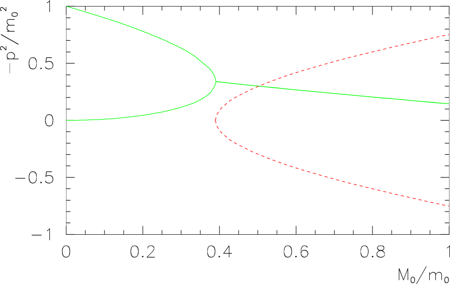
The idea to understand quark confinement is strongly linked to the expected behavior of the roots of the gap equation (32), i.e. the poles of the quark propagator. The idea presented here is identical with the idea presented in Ref. Rezaeian:2004nf , though without employing a general model for the non-locality. To represent physical propagating degrees of freedom, for these poles one should expect solutions on the real axis. The effect of the gluonic interaction is to move such poles in the complex plane so that no decay into such degrees of freedom is ever expected and the free quarks never propagate. This moves the solution from a chiral condensate phase to a confining phase for quarks at increasing coupling. Indeed, a full comprehension of such roots can only be achieved through the non-approximated gluon propagator $\tilde{\Delta}(p)$ . Therefore, we performed an analysis of the lowest zero of $\tilde{\Delta}(p)$ , finding out that for $M_{0}<0.39m_{0}$ there are two distinct real zeros while above these two zeros are given by two complex conjugate numbers. This can be seen in Fig. 1. The threshold at $0.39m_{0}$ should be seen as the point beyond which, mathematically speaking, a chiral condensate could possibly appear. We observe that the result depends critically on the mass gap value $m_{0}$ . In turn, this value depends on an arbitrary integration constant and, therefore, should be fixed by the experiment. This situation is similar to that of the constant $\Lambda$ entering in asymptotic freedom, and it is possible that these two constants are related. Our best choice to fix this value is via the mixed gluonic-quark state f₀(500) that could in principle be identified with the $\sigma$ meson in the NJL model, giving rise to the breaking of chiral symmetry.

Refer to caption — Figure 1: The two lowest zeros of $-p^{2}=M_{q}(p)$ in Euclidean domain in units of $m_{0}^{2}$ , splitted into real parts (green straight lines) and imaginary parts (red dashed lines), in dependence on the ratio $M_{0}/m_{0}$ . The zeros become complex for approximately $M_{0}/m_{0}>0.39$ .

The gap equation (32) can be simplified by choosing $m_{q}=0$ , and the factor $M_{q}$ can be cancelled from the numerator to remove the trivial case. This technique permits to find the fixed point solution of the given iterative integral equation avoiding the awkward issue to resum all the iterates. One obtains

$\displaystyle 1$	$\displaystyle=$	$\displaystyle C\alpha_{s}\int_{0}^{\Lambda^{2}}\frac{\Delta(p^{\prime})p^{\prime 2}dp^{\prime 2}}{p^{\prime 2}+M_{0}^{2}}\ =\ C\alpha\sum_{n=0}^{\infty}\int_{0}^{\Lambda^{2}}\frac{B_{n}p^{\prime 2}dp^{\prime 2}}{(p^{\prime 2}+(2n+1)^{2}m_{0}^{2})(p^{\prime 2}+M_{0}^{2})}$
	$\displaystyle=$	$\displaystyle C\alpha_{s}\sum_{n=0}^{\infty}\int_{0}^{\Lambda^{2}}\frac{B_{n}dp^{\prime 2}}{(2n+1)^{2}m_{0}^{2}-M_{0}^{2}}\left(\frac{(2n+1)^{2}m_{0}^{2}}{p^{\prime 2}+(2n+1)^{2}m_{0}^{2}}-\frac{M_{0}^{2}}{p^{\prime 2}+M_{0}^{2}}\right)$
	$\displaystyle=$	$\displaystyle C\alpha_{s}\sum_{n=0}^{\infty}\frac{B_{n}}{(2n+1)^{2}m_{0}^{2}-M_{0}^{2}}\left((2n+1)^{2}m_{0}^{2}\ln\left(1+\frac{\Lambda^{2}}{(2n+1)^{2}m_{0}^{2}}\right)-M_{0}^{2}\ln\left(1+\frac{\Lambda^{2}}{M_{0}^{2}}\right)\right).\kern-6.0pt$

For $\Lambda=1{\rm\,GeV}$ and $m_{0}=0.512(15){\rm\,GeV}$ one obtains $M_{0}=0.427(29){\rm\,GeV}$ as in Ref. Frasca:2021yuu which is clearly above the threshold $0.39m_{0}=0.2{\rm\,GeV}$ and, therefore, indicates quark confinement.

III.1 Understanding quark confinement

As we have seen, with increasing coupling of the theory the quark confinement arises at the point where the chiral condensates of different flavors perform a transition to a confined phase with an instanton liquid of gluon degrees of freedom. Neglecting the bare quark masses we have found the critical effective quark mass for which such a transition happens. Our choice of the ground state for the gluon field represents quite well a Fubini instanton Fubini:1976jm . Therefore, we expect that the chiral condensate changes into an instanton ground state that could condensate into a liquid.

The presence of the instanton liquid removes single quarks from the physical spectrum of the theory. From the mathematical point of view this means that the poles in the quark propagator become complex. The vacuum of the theory appears to undergo a series of phase transitions while the gluon sector generates a mass gap by itself in a dynamical way. The presence of the mass gap in the gluon sector is pivotal for the appearance of the phase transitions in the quark sector and, in the last instance, to the confinement of quarks.

IV Conclusions and Outlook

There are different approaches to understand the confinement of quarks. One of these is given by solutions of the gap equation of the dynamical quark mass. With a reasonable UV cutoff of $\Lambda=1{\rm\,GeV}$ and the glueball spectrum starting at the mass $m_{0}=0.512(15){\rm\,GeV}$ of the $f_{0}(500)$ resonance, the gap equation provides a value $M_{0}=0.427(29){\rm\,GeV}$ for the dynamical quark mass which turns out to be too large to allow for real valued poles of the quark propagator. As a consequence, free quarks are no longer physical states of the theory and the quarks can be expected to be confined. Even though the multiple approximations applied in this approach do not allow for quantitative estimates, we have shown how this scenario is realized in the low-energy regime of QCD by taking into account the ’t Hooft limit. By doing so, the low-energy limit of QCD turns out to be a well-defined non-local NJL model with all the parameters obtained from QCD. This entails a scenario where several condensates are formed that are expected to provide confinement in a regime of very low momentum and strong coupling.

Having a low-energy limit of QCD permits to do several computations to be compared with experiments. Indeed, our first application was to the $g-2$ problem Frasca:2021yuu with a very satisfactory agreement with data. Further research has to show whether and to what extent our description of quark confinement depends on the given parameter values and whether a stricter derivations of observables allows for a comparison with experiments.

V Acknowledgements

The research was supported in part by the European Regional Development Fund under Grant No. TK133.

References

(1) J. Greensite, “An introduction to the confinement problem,” Lect. Notes Phys. 821, (Springer, Berlin, 2011).
(2) J. B. Kogut and M. A. Stephanov, “The phases of quantum chromodynamics: From confinement to extreme environments,” (Cambridge University Press, Cambridge, 2004).
(3) K. G. Wilson, “Confinement of Quarks,” Phys. Rev. D 10, 2445-2459 (1974).
(4) T. Kugo and I. Ojima, “Local Covariant Operator Formalism of Nonabelian Gauge Theories and Quark Confinement Problem,” Prog. Theor. Phys. Suppl. 66, 1 (1979).
(5) T. Kugo and I. Ojima, “Manifestly Covariant Canonical Formulation of Yang–Mills Field Theories: Physical State Subsidiary Conditions and Physical S Matrix Unitarity,” Phys. Lett. 73B, 459 (1978).
(6) K. Nishijima, “Confinement of quarks and gluons,” Int. J. Mod. Phys. A 9, 3799 (1994).
(7) K. Nishijima, “Confinement of quarks and gluons. 2,” Int. J. Mod. Phys. A 10, 3155 (1995).
(8) M. Chaichian and K. Nishijima, “Renormalization constant of the colour gauge field as a probe of confinement,” Eur. Phys. J. C 22, 463 (2001).
(9) M. Chaichian and K. Nishijima, “Does colour confinement imply massive gluons?,” Eur. Phys. J. C 47, 737 (2006).
(10) K. Nishijima and A. Tureanu, “Gauge-dependence of Green’s functions in QCD and QED,” Eur. Phys. J. C 53, 649 (2008).
(11) N. Seiberg and E. Witten, “Monopoles, duality and chiral symmetry breaking in N=2 supersymmetric QCD,” Nucl. Phys. B 431, 484 (1994).
(12) N. Seiberg and E. Witten, “Electric - magnetic duality, monopole condensation, and confinement in N=2 supersymmetric Yang–Mills theory,” Nucl. Phys. B 426, 19 (1994); Erratum: [Nucl. Phys. B 430, 485 (1994)].
(13) V. A. Novikov, M. A. Shifman, A. I. Vainshtein and V. I. Zakharov, “Exact Gell-Mann-Low Function of Supersymmetric Yang–Mills Theories from Instanton Calculus,” Nucl. Phys. B 229, 381 (1983).
(14) M. A. Shifman and A. I. Vainshtein, “Solution of the Anomaly Puzzle in SUSY Gauge Theories and the Wilson Operator Expansion,” Nucl. Phys. B 277, 456 (1986); [Sov. Phys. JETP 64, 428 (1986)]; [Zh. Eksp. Teor. Fiz. 91, 723 (1986)].
(15) T. A. Ryttov and F. Sannino, “Supersymmetry inspired QCD beta function,” Phys. Rev. D 78, 065001 (2008).
(16) M. Chaichian and M. Frasca, “Condition for confinement in non-Abelian gauge theories,” Phys. Lett. B 781, 33 (2018).
(17) A. Hasenfratz, C. T. Peterson, J. van Sickle and O. Witzel, “ $\Lambda$ parameter of the SU(3) Yang-Mills theory from the continuous $\beta$ function,” Phys. Rev. D 108, no.1, 014502 (2023).
(18) M. Chaichian and T. Kobayashi, “On different criteria for confinement,” Phys. Lett. B 481, 26 (2000).
(19) V. N. Gribov, “Quantization of Nonabelian Gauge Theories,” Nucl. Phys. B 139, 1 (1978).
(20) D. Zwanziger, “Local and Renormalizable Action From the Gribov Horizon,” Nucl. Phys. B 323, 513 (1989).
(21) I. L. Bogolubsky, E. M. Ilgenfritz, M. Muller-Preussker, A. Sternbeck, “The Landau gauge gluon and ghost propagators in 4D SU(3) gluodynamics in large lattice volumes,” PoS LAT2007, 290 (2007).
(22) A. Cucchieri, T. Mendes, “What’s up with IR gluon and ghost propagators in Landau gauge? A puzzling answer from huge lattices,” PoS LAT2007, 297 (2007).
(23) O. Oliveira, P. J. Silva, E. M. Ilgenfritz, A. Sternbeck, “The Gluon propagator from large asymmetric lattices,” PoS LAT2007, 323 (2007).
(24) B. Lucini, M. Teper and U. Wenger, “Glueballs and k-strings in SU(N) gauge theories: Calculations with improved operators,” JHEP 0406, 012 (2004).
(25) Y. Chen et al., “Glueball spectrum and matrix elements on anisotropic lattices,” Phys. Rev. D 73, 014516 (2006).
(26) J. M. Cornwall, “Dynamical Mass Generation in Continuum QCD,” Phys. Rev. D 26, 1453 (1982).
(27) J. M. Cornwall, J. Papavassiliou, D. Binosi, “The Pinch Technique and its Applications to Non-Abelian Gauge Theories”, (Cambridge University Press, Cambridge, 2010).
(28) D. Dudal, J. A. Gracey, S. P. Sorella, N. Vandersickel and H. Verschelde, “A Refinement of the Gribov-Zwanziger approach in the Landau gauge: Infrared propagators in harmony with the lattice results,” Phys. Rev. D 78, 065047 (2008).
(29) M. Frasca, “Infrared Gluon and Ghost Propagators,” Phys. Lett. B 670, 73 (2008).
(30) M. Frasca, “Mapping a Massless Scalar Field Theory on a Yang–Mills Theory: Classical Case,” Mod. Phys. Lett. A24, 2425-2432 (2009).
(31) M. Frasca, “Quantum Yang–Mills field theory,” Eur. Phys. J. Plus 132, no. 1, 38 (2017); Erratum: [Eur. Phys. J. Plus 132, no. 5, 242 (2017)].
(32) I. L. Bogolubsky, E. M. Ilgenfritz, M. Muller-Preussker, A. Sternbeck, “Lattice gluodynamics computation of Landau gauge Green’s functions in the deep infrared,” Phys. Lett. B676, 69-73 (2009).
(33) A. G. Duarte, O. Oliveira and P. J. Silva, “Lattice Gluon and Ghost Propagators, and the Strong Coupling in Pure SU(3) Yang–Mills Theory: Finite Lattice Spacing and Volume Effects,” Phys. Rev. D 94, no. 1, 014502 (2016).
(34) A. Deur, S. J. Brodsky and G. F. de Teramond, “The QCD Running Coupling,” Prog. Part. Nucl. Phys. 90, 1 (2016).
(35) T. Schäfer and E. V. Shuryak, “Instantons in QCD,” Rev. Mod. Phys. 70, 323-426 (1998).
(36) P. Boucaud, F. De Soto, A. Le Yaouanc, J. P. Leroy, J. Micheli, H. Moutarde, O. Pene and J. Rodriguez-Quintero, “The Strong coupling constant at small momentum as an instanton detector,” JHEP 0304, 005 (2003).
(37) A. Deur, “Self-interacting scalar fields at high-temperature,” Eur. Phys. J. C 77, no. 6, 412 (2017).
(38) M. Frasca, “Confinement in a three-dimensional Yang–Mills theory,” Eur. Phys. J. C 77, no. 4, 255 (2017).
(39) G. ’t Hooft, “A Planar Diagram Theory for Strong Interactions,” Nucl. Phys. B 72, 461 (1974).
(40) G. ’t Hooft, “A Two-Dimensional Model for Mesons,” Nucl. Phys. B 75, 461-470 (1974).
(41) S. J. Brodsky, C. D. Roberts, R. Shrock and P. C. Tandy, “Confinement contains condensates,” Phys. Rev. C 85, 065202 (2012).
(42) M. Frasca, “Spectrum of Yang-Mills theory in 3 and 4 dimensions,” Nucl. Part. Phys. Proc. 294-296, 124 (2018).
(43) S. Narison, “QCD as a Theory of Hadrons: From Partons to Confinement,” Camb. Monogr. Part. Phys. Nucl. Phys. Cosmol. 17, 1-812 (2007).
(44) S. Narison, “Di-gluonium sum rules, $I=0$ scalar mesons and conformal anomaly,” Nucl. Phys. A 1017, 122337 (2022).
(45) A. Windisch, M. Q. Huber and R. Alkofer, “On the analytic structure of scalar glueball operators at the Born level,” Phys. Rev. D 87, no.6, 065005 (2013).
(46) A. Dynin, “Mathematical quantum Yang-Mills theory revisited,” Russ. J. Math. Phys. 24, 19–36 (2017).
(47) M. Frasca, A. Ghoshal and S. Groote, “Nambu-Jona-Lasinio model correlation functions from QCD,” [arXiv:2109.06465 [hep-ph]]. Contribution to QCD 21 (Montpellier, France), to appear.
(48) M. Frasca, A. Ghoshal and S. Groote, “Novel evaluation of the hadronic contribution to the muon’s g-2 from QCD,” Phys. Rev. D 104, no.11, 114036 (2021).
(49) Y. Nambu and G. Jona-Lasinio, “Dynamical Model of Elementary Particles Based on an Analogy with Superconductivity. 1.,” Phys. Rev. 122, 345-358 (1961).
(50) Y. Nambu and G. Jona-Lasinio, “Dynamical Model of Elementary Particles Based on an Analogy with Superconductivity. 2.,” Phys. Rev. 124, 246-254 (1961).
(51) S. P. Klevansky, “The Nambu-Jona-Lasinio model of quantum chromodynamics,” Rev. Mod. Phys. 64, 649 (1992).
(52) D. Gomez Dumm, A. G. Grunfeld and N. N. Scoccola, “On covariant nonlocal chiral quark models with separable interactions,” Phys. Rev. D 74, 054026 (2006).
(53) R. T. Cahill and C. D. Roberts, “Soliton Bag Models of Hadrons from QCD,” Phys. Rev. D 32, 2419 (1985).
(54) C. D. Roberts and R. T. Cahill, “Dynamically Selected Vacuum Field Configuration in Massless QED,” Phys. Rev. D 33, 1755 (1986).
(55) C. D. Roberts and R. T. Cahill, “A Bosonization of QCD and Realizations of Chiral Symmetry,” Austral. J. Phys. 40, 499 (1987).
(56) J. Praschifka, C. D. Roberts and R. T. Cahill, “QCD Bosonization and the Meson Effective Action,” Phys. Rev. D 36, 209 (1987).
(57) T. Hell, S. Rössner, M. Cristoforetti, W. Weise, “Dynamics and thermodynamics of a non-local PNJL model with running coupling,” Phys. Rev. D79 (2009) 014022.
(58) D. Ebert, “Bosonization in particle physics,” Lect. Notes Phys. 508, 103-114 (1998).
(59) R. D. Bowler and M. C. Birse, “A Nonlocal, covariant generalization of the NJL model,” Nucl. Phys. A 582, 655 (1995).
(60) C. D. Roberts and A. G. Williams, “Dyson-Schwinger equations and their application to hadronic physics,” Prog. Part. Nucl. Phys. 33, 477-575 (1994).
(61) C. M. Bender, K. A. Milton and V. M. Savage, “Solution of Schwinger-Dyson equations for PT symmetric quantum field theory,” Phys. Rev. D 62 (2000) 085001.
(62) M. Frasca, “Differential Dyson–Schwinger equations for quantum chromodynamics,” Eur. Phys. J. C 80, 707 (2020).
(63) M. Frasca, “Scalar field theory in the strong self-interaction limit,” Eur. Phys. J. C 74 (2014) 2929.
(64) M. Frasca, “ $\rho$ condensation and physical parameters,” JHEP 11, 099 (2013).
(65) M. Frasca, “Finite temperature corrections to a NLO Nambu-Jona-Lasinio model,” Nucl. Part. Phys. Proc. 282-284, 173-176 (2017).
(66) M. Frasca, “Exact solutions of classical scalar field equations,” J. Nonlin. Math. Phys. 18, no.2, 291-297 (2011).
(67) S. Fubini, “A New Approach to Conformal Invariant Field Theories,” Nuovo Cim. A 34, 521 (1976).
(68) A. H. Rezaeian, N. R. Walet and M. C. Birse, “Baryon structure in a quark-confining non-local NJL model,” Phys. Rev. C 70, 065203 (2004).