152
\jmlryear2021
\jmlrworkshopConformal and Probabilistic Prediction and Applications
\jmlrproceedingsPMLRProceedings of Machine Learning Research
\editorLars Carlsson, Zhiyuan Luo, Giovanni Cherubin and Khuong An Nguyen
\theorembodyfont
\theoremheaderfont
\theorempostheader:
\theoremsep
Conformal Uncertainty Sets for Robust Optimization
Abstract
Decision-making under uncertainty is hugely important for any decisions sensitive to perturbations in observed data. One method of incorporating uncertainty into making optimal decisions is through robust optimization, which minimizes the worst-case scenario over some uncertainty set. We connect conformal prediction regions to robust optimization, providing finite sample valid and conservative ellipsoidal uncertainty sets, aptly named conformal uncertainty sets. In pursuit of this connection we explicitly define Mahalanobis distance as a potential conformity score in full conformal prediction. We also compare the coverage and optimization performance of conformal uncertainty sets, specifically generated with Mahalanobis distance, to traditional ellipsoidal uncertainty sets on a collection of simulated robust optimization examples.
keywords:
Uncertainty quantification, multi-target regression, prediction regions, stochastic optimization, conformal prediction, constrained optimization.1 Introduction
In many settings, the act of quantifying uncertainty related to some predicted outcome is just as important as the prediction itself. Prediction intervals allow for the attachment of bounds on random variables of interest, that tell us, with a specified probability, where observations of said random variables could fall. Ideally, we wish to construct a prediction interval such that
| (1) |
where is our random variable of interest, and is our desired error rate. In more complex settings, it might be of interest to capture multiple responses with a specified probability. Thus, we might construct a prediction region such that (1) holds for and some -dimensioned version of , say . Our discussion focuses on generating finite sample valid and distribution free prediction regions through conformal prediction (Gammerman et al., 1998; Vovk et al., 2005).
The importance of generating intervals (or regions) to accompany point predictions cannot be overstated. However, the role of these uncertainty estimates in a decision-making framework is not always explicit (Reckhow, 1994). While some situations dictate an intuition-based response to uncertainty, e.g., a person avoiding an object while driving, other situations might call for a more tangible use of uncertainty estimates, e.g., assessing potential customer demand for a product (Bertsimas and Thiele, 2006). Multiple decision-making methods exist which explicitly take into account uncertainty, e.g., utility theory (Fishburn, 1968) and risk-based decision-making (Lounis and McAllister, 2016), but in our discussion we focus on one specific method for incorporating uncertainty into the decision-making process: robust optimization (Ben-Tal et al., 2009).
Robust optimization allows for the explicit utilization of uncertainty quantification in the construction of optimal and risk-averse decisions, specifically in a constrained environment. Formally, a robust optimization formulation generates an optimal solution to the problem,
| (2) |
delivering some decision that minimizes the worst-case of some objective function , subject to a feasible region and an uncertainty set for random parameters . The uncertainty set(s) within a robust optimization formulation are meant to act as “knob” to adjust the risk-averse nature of a decision, with larger uncertainty sets associated with a higher degree of risk-aversion.
Given that the uncertainty set is meant to control the risk associated with a random set of parameters, their construction could benefit from the theoretical results inherent to conformal prediction. Thus, we propose a new methodological connection between conformal prediction and robust optimization. Specific contributions of the paper are listed below:
-
•
We explicitly define Mahalanobis distance as a multivariate conformity score in the full conformal prediction case. We also generalize Mahalanobis distance to be constructed in conjunction with any univariate conformity score.
-
•
We introduce conformal uncertainty sets, which provide finite sample valid and distribution free uncertainty sets within the robust optimization framework.
-
•
We also construct a small robust optimization example as a proof-of-concept for the use of conformal uncertainty sets, specifically with Mahalanobis distance as our conformity score of choice.
Overall, we see that conformal uncertainty sets provide a new avenue for the construction of uncertainty sets. Additionally, we see from simulated cases that conformal uncertainty sets are competitive with traditional uncertainty sets.
In Section 2 we discuss relevant background to our work. Section 3 introduces the conformal approach for generating uncertainty and discusses issues that arise with full conformal prediction. Section 4 relays empirical results to assess the validity, efficiency, and overall performance of conformal uncertainty sets. Section 5 concludes the paper.
2 Background
In this section we provide background on relevant topics for this paper. These topics include: conformal prediction, joint prediction regions and robust optimization.
2.1 Conformal Prediction
Conformal prediction was first introduced in Gammerman et al. (1998) as a method for quantifying uncertainty in both classification and regression tasks. Vovk et al. (2005) provides a formalized introduction to conformal prediction as well as application (and associated theoretical results) in multiple data settings, e.g., online and batch procedures.
We define as a collection of observations, where the -th data tuple is made up of a covariate vector and a response . Our goal is to utilize in some fashion to construct a valid prediction interval for a new observation , where is some known covariate vector and is some, yet-to-be-observed response. Assuming each data pair and are drawn exchangeably from some distribution , conformal prediction generates conservative, finite sample valid prediction intervals in a distribution-free manner. Specifically, prediction intervals are generated through the repeated inversion of the test,
| (3) | ||||
where is a potential candidate response value for , i.e., the null hypothesis (Lei et al., 2018).
In a prediction setting, the test inversion is achieved by refitting the prediction model of interest with an augmented data set including a new data tuple . Following the refitting, each observation in the augmented data set receives a (non)conformity score, which determines the level of (non)conformity between itself and other observations. In general, a conformity score can be any measurable function. For example, one popular conformity score is the absolute residual
| (4) |
where is the predicted value for generated using the augmented data set. While the prediction is dependent on both and , we omit dependence on and in our notation.
For each candidate value we construct ,
| (5) |
where is the conformity score associated with the data pair and is the conformity score associated with . Informally, is the proportion of observations in the augmented data set whose conformity score is less than or equal to the conformity score associated with candidate value .
The conformal prediction region for the incoming response is,
| (6) |
In order to make the construction of a tractable problem, each candidate value is chosen from a finite grid of points in , defined as the set . With previous results shown in Vovk et al. (2005) and Lei et al. (2018), provides a prediction interval such that
| (7) |
for any . The left-hand side of the inequality holds under exchangeability, while the right-hand side holds under the additional assumption of unique and continuous conformity scores. Thus, conformal prediction intervals are conservative, but not too conservative, while maintaining finite sample validity.
With “full” conformal prediction, each new candidate value for the response associated with requires an additional prediction model to be fit using the augmented data set, which is computationally expensive. An alternative method, dubbed “split” conformal prediction, utilizes an adjusted approach to full conformal prediction, but reduces the computational load required, while still achieving the same finite sample results. For clarity, we differentiate the two methods by specifically referencing them as “full” and “split”, respectively, for the remainder for the paper.
Under the same assumptions of exchangeability, split conformal prediction only necessitates fitting the model once. The training data set is partitioned into two sets, and . A prediction model is fit using and then conformity scores are generated for each observation in . Then, the prediction interval constructed with split conformal prediction is
| (8) |
where is the prediction for generated using the observations in , and is the -th largest conformity score value for observations in .
A non-exhaustive subset of CP extensions include Mondrian conformal prediction (Boström and Johansson, 2020), jackknife+ (Barber et al., 2021), aggregated conformal inference (Carlsson et al., 2014), distributional conformal prediction (Chernozhukov et al., 2019) and change detection through conformal martingales (Volkhonskiy et al., 2017). Advances towards conditionally valid coverage are discussed in Vovk (2012), Guan (2019) and Barber et al. (2019), among others. For an extensive (and more recent) review of conformal prediction advances, we point the interested reader to Zeni et al. (2020).
2.2 Joint Prediction Regions
Instead of quantifying uncertainty for individual points, e.g., with prediction intervals, one might desire to quantify uncertainty for a collection of points. In a marginal sense, we can use simultaneous prediction intervals to, say, contain a collection of observations with some probability . Thus, we might construct an interval such that,
| (9) |
Unfortunately, generating prediction intervals for observations where the distribution is unknown is not a straightforward task. One method traditionally used to deliver conservative simultaneous prediction intervals is through the Bonferroni inequality,
| (10) |
which holds regardless of the dependency between responses (Bonferroni, 1936). If we construct such that
where , then and we have a conservative, simultaneous prediction interval.
Obviously, the construction of a single prediction interval to contain a collection of points only makes sense if the observations are identically distributed. In the case of multi-target regression, where we are interested in multiple responses, this is not necessarily the case. Thus, it would be beneficial to construct a prediction region to quantify uncertainty associated with a collection of responses jointly, rather than marginally.
While many methods exist for generating prediction regions, e.g., bootstrap prediction regions (Beran, 1992) and Bayesian prediction regions (Datta et al., 2000), our work builds from results in Scheffé (1959), which introduces a prediction region for a vector of responses ,
where is the mean of the random vector , is the inverse-covariance matrix of and is the -th quantile associated with the distribution with degrees of freedom. In practice, the true mean and covariance are usually unknown. Thus, we replace and with their estimates, and , respectively, resulting in a prediction region
| (11) |
which is asymptotically valid. Our focus on generating conformal prediction regions in a similar fashion is purely pragmatic as it supports the connection of conformal prediction regions to robust optimization, which we provide background on in Section 2.3.
The first results extending conformal prediction to the multivariate response case (to our knowledge) come from Lei et al. (2015), which applies conformal prediction to functional data, providing bounds associated with prediction “bands”. Diquigiovanni et al. (2021) extends and generalizes additional results for conformal prediction on functional data.
The functional case is inherently multidimensional and can be applied to a prediction region setting, but more focused work on prediction regions also exists. Joint conformal prediction regions were explicitly introduced in Kuleshov et al. (2018) and Neeven and Smirnov (2018). More recent advances include Messoudi et al. (2020), which delivers Bonferroni-type prediction intervals through neural networks. Messoudi et al. (2021) extends this work through the use of copula-based conformal prediction. Cella and Martin (2020) use Tukey’s half-space depth (Tukey, 1975) as a conformity score for the multivariate response case. Kuchibhotla (2020) explicitly describes conformal regions for arbitrary spaces, delivering theoretical results to support the validity of conformal prediction regions in . Chernozhukov et al. (2018) provides valid conformal prediction regions for potentially dependent data, generalizing the traditional conformal inference assumption of exchangeability.
2.3 Robust Optimization
While real-world decision-making requires simplifying assumptions, the assumption of data certainty can be a damaging one. When constructing a formulation for an optimization problem, parameters in the formulation might come from subject matter expertise, historical data or even physical limitations. However, small perturbations in these values might not only result in the current solution being suboptimal, but also potentially infeasible (Ben-Tal and Nemirovski, 2002).
Stochastic optimization (Shapiro et al., 2014) aims to take uncertainties into account within a decision-making process. For some set of decision variables , a stochastic optimization problem might take the form,
| (12) |
where is the feasible region, is the objective function, and is a vector of random parameters we do not observe until our decision timeline is over. While not denoted explicitly, the feasible region might also depend on . For our discussion, we assume is independent of the random parameters.
Under the stochastic optimization framework, there are multiple approaches to address uncertainty. A subset includes chance-constrained programming (Charnes and Cooper, 1959; Miller and Wagner, 1965), sample-average approximation (Kleywegt et al., 2002) and robust optimization (Ben-Tal et al., 2009; Bertsimas et al., 2011). We limit further discussion to the latter.
In order to incorporate uncertainty into the optimization framework, robust optimization (RO) utilizes uncertainty sets on the random parameters, solving the problem,
| (13) |
Thus, RO minimizes the potential worst-case outcome with respect to the uncertainty set . Uncertainty sets can be constructed in either a naive (without data), or a data-driven manner. Without observations of the random parameters we can assume interval constraints associated with each element of , constructing an uncertainty set ,
| (14) |
with some lower and upper endpoints, and , respectively. Barring pathological cases, the use of in convex optimization results in each of the uncertain elements obtaining some boundary value. Given a historical data set of observed uncertain parameters we can also provide data-driven, norm-based uncertainty sets,
| (15) |
where is the -norm, is the vector of sample means associated with observations of the uncertain parameters, and is some budget of uncertainty. Bertsimas and Thiele (2006) highlight that data-driven uncertainty sets like (15) outperform “naive” uncertainty sets like (14). Selecting with results in a strictly spherical uncertainty set. Adjusting the errors by some matrix allows for the construction of ellipsoidal uncertainty sets,
| (16) |
For our discussion, we focus our discussion on ellipsoidal uncertainty sets.
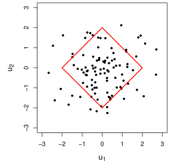
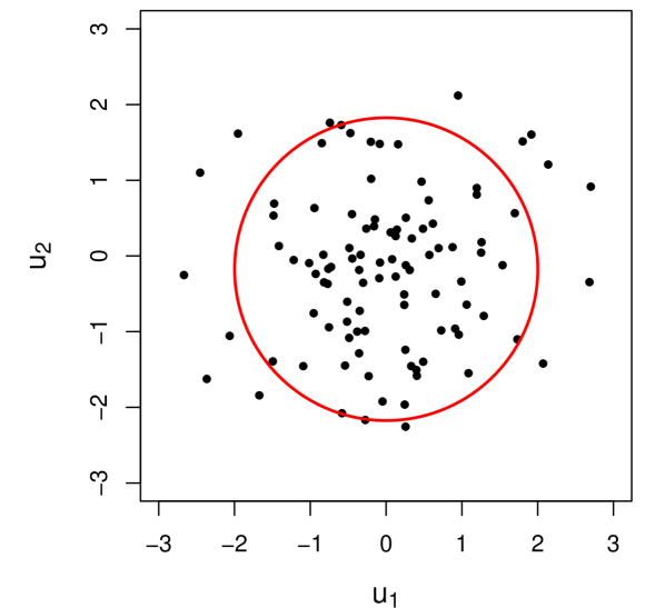
A larger value of corresponds to a more risk-averse decision. Thus, a trade-off exists between the optimal solution and the “robustness” of said solution. Figure 1 shows examples of norm-based uncertainty sets constructed with different values for for a two-dimensional data set drawn from two independent standard normal random variables.
To solidify the intuition behind robust optimization we construct a toy example. Suppose we have the vector of decision variables and a vector of random parameters . In this case our random parameter vector is some cost and our goal is to minimize said cost. For this example, we assume to be multivariate normal with mean equal to the zero vector and covariance matrix with marginal variance of one and correlation of . The robust optimization formulation of interest is,
| (17) |
where and is the lower triangular matrix of the Cholesky decomposition for the inverse-covariance matrix associated with .
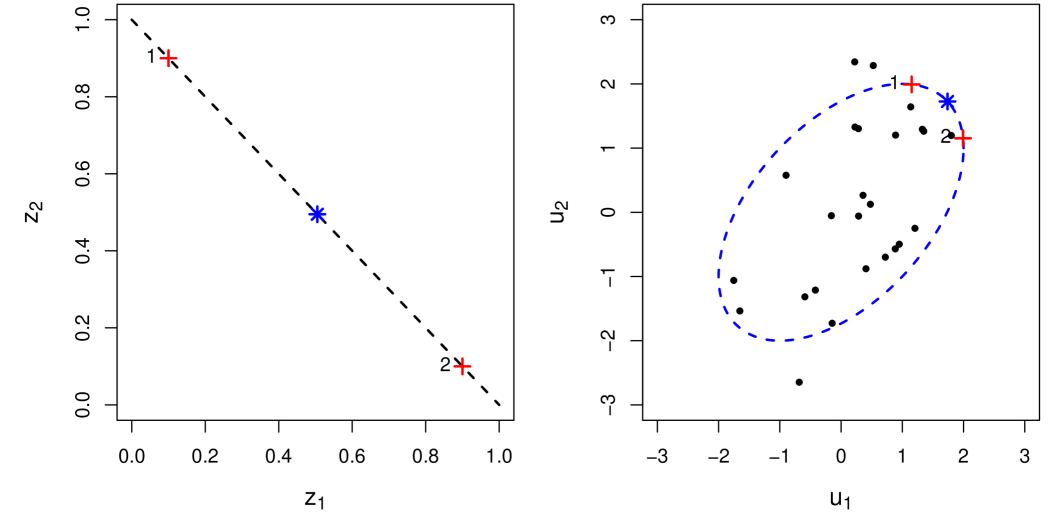
The intuition behind (17) is illustrated in Figure 2. In the left plot we show the feasible region for as the dotted line from to . Along the feasible region we identify two sub-optimal feasible solutions at and with red plusses. In the right plot we identify the border of the uncertainty set with the blue dotted line. We also denote the worst-case value of for each sub-optimal feasible solution identified in the left plot, and respectively, with red plusses. Twenty-five sample observations of are also shown. The optimal solution at , along with the corresponding worst-case realization, , are identified with blue asterisks.
Even though most robust optimization problems are inherently more difficult to solve than, say, linear optimization problems, tractable formulations do exist. Intimate details of of these tractable implementations are not crucial to our discussion. Additional insight on robust optimization as well as practical applications can be seen in Bertsimas et al. (2011) and Gorissen et al. (2015), among others.
3 Conformal Uncertainty Sets for Robust Optimization
Other works, e.g., Bertsimas et al. (2018), Delage and Ye (2010), Chen et al. (2010) and Lu (2011), have reduced the distributional assumptions required to generate uncertainty sets with better probabalistic guarantees, but these results still rely on distributional assumptions of the data and/or on some large sample requirement.
In this section we explore Mahalanobis distance as a conformity score for multivariate responses and connect to uncertainty sets for robust optimization. For completeness, we define and generalize Mahalanobis distance for use in full conformal prediction. In Section 3.2, we shift our focus to split conformal prediction.
3.1 Conformal Prediction with Mahalanobis Distance
Instead of making assumptions on the normality of our variables of interest and/or if we have enough observations for large sample approximations, we can use conformal prediction to generate finite sample, distribution free prediction regions for any set of multivariate random variables.
3.1.1 Full Conformal Approach
Suppose again we define as a collection of observations. In this case, the -th data tuple is made up of a covariate vector and a response vector , which slightly differs from the tuple construction in Section 2.1. We also assume each data tuple and our new observation , where , are drawn exchangeably from some distribution .
The prediction region of interest is one which contains the new response with probability . We define a candidate value vector and as the estimate of , constructed using the augmented data set. Instead of a univariate conformity score, e.g., the absolute residual for a candidate response value, we can construct a multivariate conformity score ,
| (18) |
where , is a univariate conformity score associated with the -th response of , and is the sample inverse-covariance matrix associated with the univariate conformity scores. We ignore the dependence of on in notation. We explicitly define as the vector of individual predictions for each element in . In our case, for a given observation we specify , the residual associated with the -th response. However, can be generally defined as any univariate conformity score. We define , with no indexing, as the conformity score associated with .
For univariate conformal prediction we utilize a set of candidate values for each new observation . The multivariate case instead requires a set of candidate values . Analogous to (5), we define a new version of utilizing (18),
| (19) |
Then, a conservative conformal prediction region is formed by
| (20) |
With as defined previously, (18) is the Mahalanobis distance between the vector and . Thus, the conformal predictions regions generated are analogous to (11). A similar version of (18) was suggested as a conformity measure for split conformal prediction in Kuchibhotla (2020). Its explicit definition in full conformal prediction is new, but also brings an increased computational burden to its use.
While it is not obvious, prediction regions generated with the full conformal approach are not necessarily ellipsoidal (or convex), which can can problems from an optimization perspective. Ben-Tal et al. (2009) show that in a convex optimization problem, we can replace any uncertainty set with its convex hull, but we do not explore this further in our discussion.
3.1.2 Split Conformal Approach
The conformity score identified in (18) can be extended to the split conformal approach. However, careful consideration must be taken when constructing . Given that split conformal requires the partitioning of the data set into and , Kuchibhotla (2020) suggested the use of , an estimate of the univariate conformity score inverse-covariance matrix generated from observations in .
With the split conformal procedure, we can generate a closed-form for our split conformal prediction region by using , the largest value of . With (18) as our conformity score, we generate a prediction region,
| (21) |
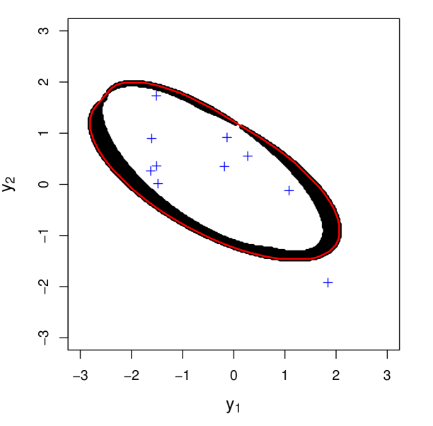
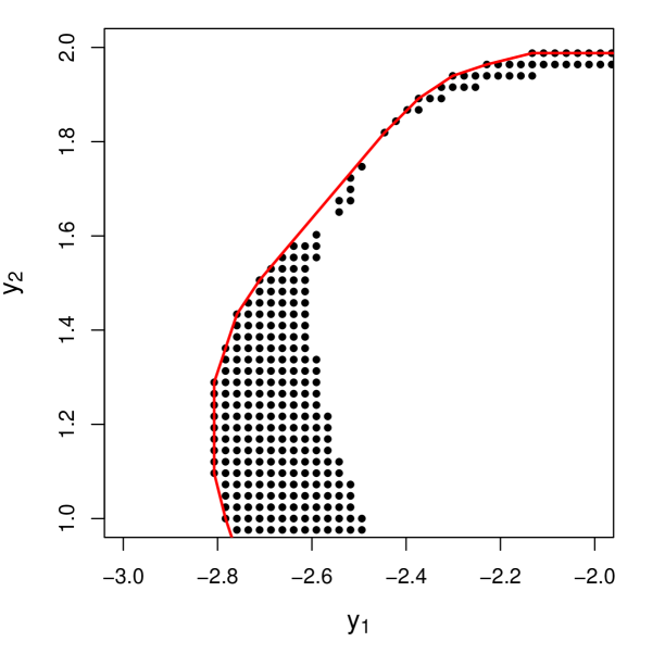
which is the split conformal equivalent of (20). Because is quadratic, is an ellipsoidal prediction region, with defining the ellipsoid border. Thus, we can construct the ellipsoidal prediction region by finding each tuple such that the equality portion of (21) holds. This differs from the univariate split conformal case, where the prediction intervals are defined explicitly by observations in .
Due to the potential lack of convexity for full conformal prediction regions constructed with Mahalanobis distance, we utilize the split conformal results for extension to uncertainty sets in Section 3.2.
3.2 Extension to Uncertainty Sets
For RO, the parameter in (15) and (16) can be chosen by a decision maker, with higher values of corresponding to higher levels of risk aversion. However, we can also select in such a way as to obtain probabilistic guarantees associated with the uncertainty set constructed, e.g., through a joint prediction region constructed under normality. With reasonable, i.e., consistent, estimates of the true mean and true covariance matrix for and selected as the square root of , (11) provides an asymptotically valid ellipsoidal uncertainty set, as long as normality holds.
In contrast to ellipsoidal uncertainty sets constructed under normality, we can also generate uncertainty sets with probabalistic bounds through split conformal prediction in a distribution free manner. While the terms “prediction region” and “uncertainty set” are normally used in the context of uncertainty quantification and robust optimization, respectively, they become equivalent in the case of conformal uncertainty sets.
By the results previously discussed, we can provide a finite sample, distribution free prediction region for through split conformal prediction. We can then use this region as a conservative uncertainty set in any robust optimization problem. Specifically, we select such that of the conformity scores constructed from are less than or equal to , guaranteeing a valid uncertainty set. We formalize the selection of for some fixed as,
| (22) |
where is constructed using (18). We require the supremum over because we are looking for the specific value associated with the border of the conformal prediction region, giving us the effective radius of our ellipsoid, which aligns exactly with the prediction region constructed in (21). Using as constructed with (22) allows for ellipsoidal uncertainty sets of the form,
| (23) |
where is the lower triangular matrix of the Cholesky decomposition for the inverse-covariance matrix associated with the conformity scores of observations in . Uncertainty sets of the form in (23) are easily implementable in currently-existing robust optimization solvers. Because (23) is constructed through split conformal prediction, we achieve the finite sample results associated with conformal prediction and can generate finite sample valid, distribution free uncertainty sets for robust optimization.
4 Performance Comparison
We compare the efficiency, coverage and performance of conformal uncertainty sets to traditional ellipsoidal uncertainty sets in a simulated setting, generalizing (17) to dimensions,
| (24) |
Three different uncertainty sets are considered: no uncertainty, ellipsoidal uncertainty under normality, and conformal ellipsoidal uncertainty. We construct a set of experiments by varying data generation schemes, the number of historical observations of the random parameter vector , the significance level , and the dimension . The different data generation schemes include:
-
•
both normally distributed, and -distributed costs
-
•
various random parameter mean-variance scenarios: 1) independent and identically distributed, 2) independent, but not identically distributed, and 3) correlated
We generate correlated, marginally -distributed random parameters through the probability integral transform of multivariate normal random variable.
For every combination of the data generation schemes above we perform experiments with varying values for , and . For each instance of an experiment we:
-
1.
Generate both training and test data according to that experiments data generation scheme and set-up (i.e., choice for , , and ).
-
2.
Using the training data we construct our uncertainty sets, and solve the robust optimization model given this training data.
-
3.
The solution of this problem provides an optimal decision variable w.r.t. the training data. We then calculate objective function values, using this optimal decision, across the test data set. This generates a distribution of objective function values (one for each entry in the test data set).
-
4.
We then calculate the quantile of this distribution and store.
-
5.
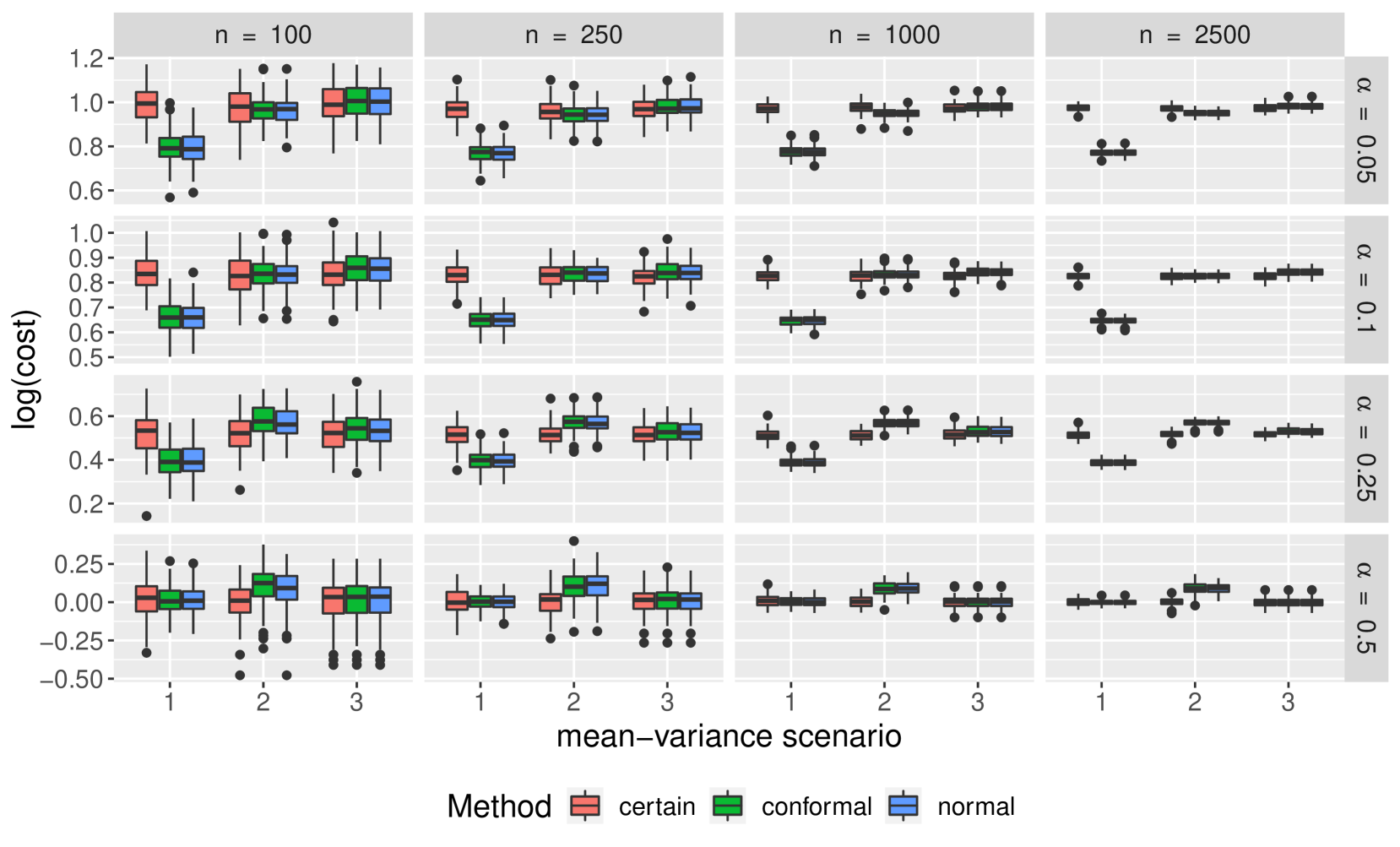
We repeat each experiment 100 times, recording the worst-case costs for each optimal decision on a test set of 250 random parameter vectors.
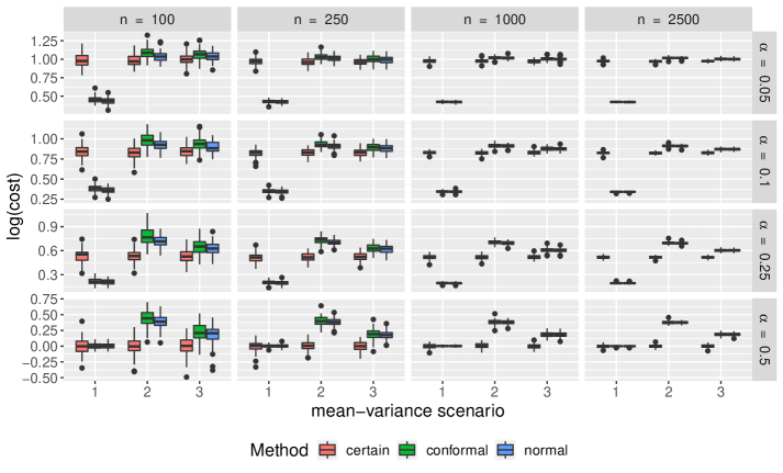
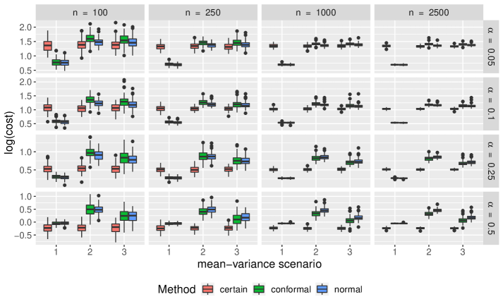
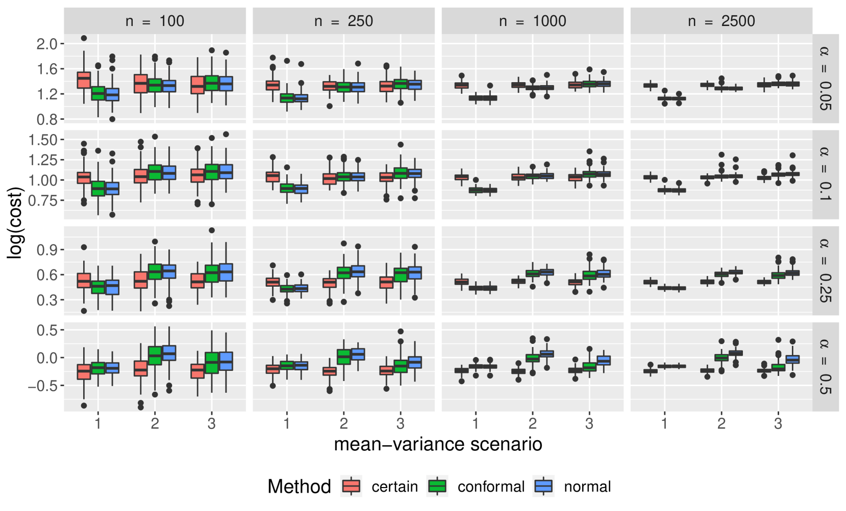
Figure 4 compares the overall robust optimization performance of the three uncertainty sets of interest in terms of worst-case performance. We see that while the conformal uncertainty sets results in worst-case scenarios comparable to uncertainty sets constructed under normality, they do not seem to be superior. We also see under mean-variance scenarios one and two, the non-robust optimization has better worst-case scenario performance than any of the robust formulations.
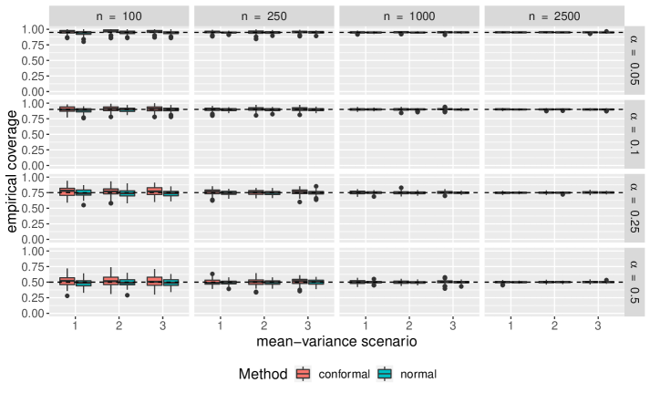
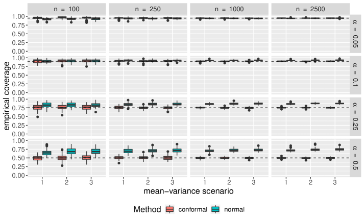
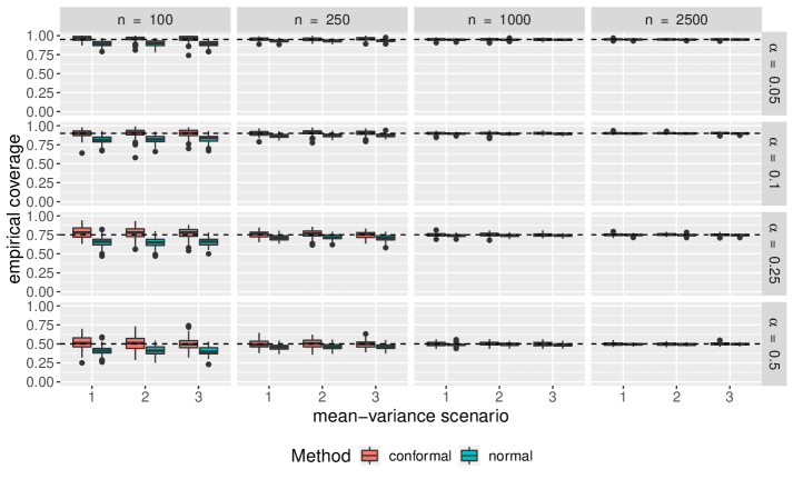
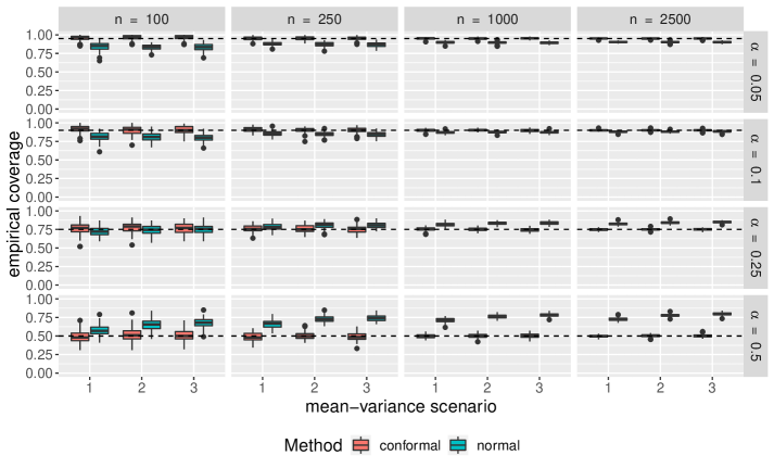
Comparisons of empirical coverage for each uncertainty set are shown in Supplementary Materials. We see the coverage for the conformal uncertainty sets is much closer to nominal in both the cases of normally distributed and -distributed random parameter vectors. While not shown, we also find conformal uncertainty sets to be more efficient than those constructed under normality.
5 Conclusion
In this paper we showed empirically the effectiveness of the Mahalanobis distance as a multivariate conformity score, specifically for the use in the generation of uncertainty sets for robust optimization. Conformal uncertainty sets not only provide finite sample validity, but are also empirically more efficient than uncertainty sets based on normality. However, more exploration is needed to assess the poor performance from a robust optimization perspective. For prediction regions, it is widely accepted that without validity, efficiency is not informative. Thus, comparing the worst-case performance of the uncertainty sets constructed when the coverage of the normality-based prediction regions is not valid, let alone conservative, is a potentially unfair one. Our comparisons also fail to describe the potential trade-off between robustness and average performance. Thus, further exploration is needed to see where conformal uncertainty sets might better perform. Additionally, in the future we hope to explore performance in a practical setting, rather than just a simulated one.
In our discussion we chose Mahalanobis distance as our sole conformity score due to the inherent relationship between itself and traditional ellipsoidal uncertainty sets. However, another conformity score, referenced in Section 2.1, is half-space depth. With half-space depth we can decompose a set of points in into a nested set of convex regions (Bremner, 2007), which would be helpful in the construction of polyhedral uncertainty sets. Future work might compare the performance of conformal uncertainty sets constructed with Mahalanobis distance and half-space depth.
We focused on a robust optimization problem where there was uncertainty only in the objective function coefficients. Applying conformal uncertainty sets to more complex robust optimization formulations, e.g., with uncertainty in the constraints, is a natural extension. Additionally, utilizing conformal prediction regions to provide probabalistic controls on constraint violation would also be useful. We also assumed independence of the feasible region and uncertain parameters . Relaxation of this assumption could be beneficial as well.
Given the attractiveness of pairing conformal prediction with prediction and classification methods, another natural extension would be conformal uncertainty sets for robust optimization with covariates. One could construct as a function of a vector of covariates ,
| (25) |
where is the prediction for the response vector given and is an estimate of the lower triangular matrix of the Cholesky decomposition for the inverse-covariance matrix of . While conformal uncertainty sets generated with covariate information would still be valid marginally, additional consideration could be taken to generate locally valid prediction regions and uncertainty sets. Locally valid prediction regions have recently been explored in Diquigiovanni et al. (2021) with respect to functional data through the use of a modulation function.
References
- Barber et al. (2019) Rina Foygel Barber, Emmanuel J Candes, Aaditya Ramdas, and Ryan J Tibshirani. The limits of distribution-free conditional predictive inference. arXiv preprint arXiv:1903.04684, 2019.
- Barber et al. (2021) Rina Foygel Barber, Emmanuel J Candes, Aaditya Ramdas, and Ryan J Tibshirani. Predictive inference with the jackknife+. The Annals of Statistics, 49(1):486–507, 2021.
- Ben-Tal and Nemirovski (2002) Aharon Ben-Tal and Arkadi Nemirovski. Robust optimization–methodology and applications. Mathematical programming, 92(3):453–480, 2002.
- Ben-Tal et al. (2009) Aharon Ben-Tal, Laurent El Ghaoui, and Arkadi Nemirovski. Robust optimization. Princeton university press, 2009.
- Beran (1992) Rudolf Beran. Designing bootstrap prediction regions. In Bootstrapping and Related Techniques, pages 23–30. Springer, 1992.
- Bertsimas and Thiele (2006) Dimitris Bertsimas and Aurélie Thiele. Robust and data-driven optimization: modern decision making under uncertainty. In Models, methods, and applications for innovative decision making, pages 95–122. INFORMS, 2006.
- Bertsimas et al. (2011) Dimitris Bertsimas, David B Brown, and Constantine Caramanis. Theory and applications of robust optimization. SIAM review, 53(3):464–501, 2011.
- Bertsimas et al. (2018) Dimitris Bertsimas, Vishal Gupta, and Nathan Kallus. Data-driven robust optimization. Mathematical Programming, 167(2):235–292, 2018.
- Bonferroni (1936) Carlo Bonferroni. Teoria statistica delle classi e calcolo delle probabilita. Pubblicazioni del R Istituto Superiore di Scienze Economiche e Commericiali di Firenze, 8:3–62, 1936.
- Boström and Johansson (2020) Henrik Boström and Ulf Johansson. Mondrian conformal regressors. In Conformal and Probabilistic Prediction and Applications, pages 114–133. PMLR, 2020.
- Bremner (2007) David Bremner. Halfspace depth: motivation, computation, optimization. 2007.
- Carlsson et al. (2014) Lars Carlsson, Martin Eklund, and Ulf Norinder. Aggregated conformal prediction. In IFIP International Conference on Artificial Intelligence Applications and Innovations, pages 231–240. Springer, 2014.
- Cella and Martin (2020) Leonardo Cella and Ryan Martin. Valid distribution-free inferential models for prediction. arXiv preprint arXiv:2001.09225, 2020.
- Charnes and Cooper (1959) Abraham Charnes and William W Cooper. Chance-constrained programming. Management science, 6(1):73–79, 1959.
- Chen et al. (2010) Wenqing Chen, Melvyn Sim, Jie Sun, and Chung-Piaw Teo. From cvar to uncertainty set: Implications in joint chance-constrained optimization. Operations research, 58(2):470–485, 2010.
- Chernozhukov et al. (2018) Victor Chernozhukov, Kaspar Wüthrich, and Zhu Yinchu. Exact and robust conformal inference methods for predictive machine learning with dependent data. In Conference On Learning Theory, pages 732–749. PMLR, 2018.
- Chernozhukov et al. (2019) Victor Chernozhukov, Kaspar Wüthrich, and Yinchu Zhu. Distributional conformal prediction. arXiv preprint arXiv:1909.07889, 2019.
- Datta et al. (2000) Gauri Sankar Datta, Malay Ghosh, Rahul Mukerjee, and Trevor J Sweeting. Bayesian prediction with approximate frequentist validity. The Annals of Statistics, 28(5):1414–1426, 2000.
- Delage and Ye (2010) Erick Delage and Yinyu Ye. Distributionally robust optimization under moment uncertainty with application to data-driven problems. Operations research, 58(3):595–612, 2010.
- Diquigiovanni et al. (2021) Jacopo Diquigiovanni, Matteo Fontana, and Simone Vantini. Conformal prediction bands for multivariate functional data. arXiv preprint arXiv:2106.01792, 2021.
- Fishburn (1968) Peter C Fishburn. Utility theory. Management science, 14(5):335–378, 1968.
- Gammerman et al. (1998) A Gammerman, V Vovk, and V Vapnik. Learning by transduction. In Proceedings of the Fourteenth conference on Uncertainty in artificial intelligence, pages 148–155, 1998.
- Gorissen et al. (2015) Bram L Gorissen, İhsan Yanıkoğlu, and Dick den Hertog. A practical guide to robust optimization. Omega, 53:124–137, 2015.
- Guan (2019) Leying Guan. Conformal prediction with localization. arXiv preprint arXiv:1908.08558, 2019.
- Kleywegt et al. (2002) Anton J Kleywegt, Alexander Shapiro, and Tito Homem-de Mello. The sample average approximation method for stochastic discrete optimization. SIAM Journal on Optimization, 12(2):479–502, 2002.
- Kuchibhotla (2020) Arun Kumar Kuchibhotla. Exchangeability, conformal prediction, and rank tests. arXiv preprint arXiv:2005.06095, 2020.
- Kuleshov et al. (2018) Alexander Kuleshov, Alexander Bernstein, and Evgeny Burnaev. Conformal prediction in manifold learning. In Conformal and Probabilistic Prediction and Applications, pages 234–253, 2018.
- Lei et al. (2015) Jing Lei, Alessandro Rinaldo, and Larry Wasserman. A conformal prediction approach to explore functional data. Annals of Mathematics and Artificial Intelligence, 74(1):29–43, 2015.
- Lei et al. (2018) Jing Lei, Max G’Sell, Alessandro Rinaldo, Ryan J Tibshirani, and Larry Wasserman. Distribution-free predictive inference for regression. Journal of the American Statistical Association, 113(523):1094–1111, 2018.
- Lounis and McAllister (2016) Zoubir Lounis and Therese P McAllister. Risk-based decision making for sustainable and resilient infrastructure systems. Journal of Structural Engineering, 142(9):F4016005, 2016.
- Lu (2011) Zhaosong Lu. Robust portfolio selection based on a joint ellipsoidal uncertainty set. Optimization Methods & Software, 26(1):89–104, 2011.
- Messoudi et al. (2020) Soundouss Messoudi, Sébastien Destercke, and Sylvain Rousseau. Conformal multi-target regression using neural networks. In Conformal and Probabilistic Prediction and Applications, pages 65–83. PMLR, 2020.
- Messoudi et al. (2021) Soundouss Messoudi, Sébastien Destercke, and Sylvain Rousseau. Copula-based conformal prediction for multi-target regression. arXiv preprint arXiv:2101.12002, 2021.
- Miller and Wagner (1965) Bruce L Miller and Harvey M Wagner. Chance constrained programming with joint constraints. Operations Research, 13(6):930–945, 1965.
- Neeven and Smirnov (2018) Jelmer Neeven and Evgueni Smirnov. Conformal stacked weather forecasting. In Conformal and Probabilistic Prediction and Applications, pages 220–233, 2018.
- Reckhow (1994) Kenneth H Reckhow. Importance of scientific uncertainty in decision making. Environmental Management, 18(2):161–166, 1994.
- Scheffé (1959) Henry Scheffé. The analysis of variance. 1959.
- Shapiro et al. (2014) Alexander Shapiro, Darinka Dentcheva, and Andrzej Ruszczyński. Lectures on stochastic programming: modeling and theory. SIAM, 2014.
- Tukey (1975) John W Tukey. Mathematics and the picturing of data. In Proceedings of the International Congress of Mathematicians, Vancouver, 1975, volume 2, pages 523–531, 1975.
- Volkhonskiy et al. (2017) Denis Volkhonskiy, Evgeny Burnaev, Ilia Nouretdinov, Alexander Gammerman, and Vladimir Vovk. Inductive conformal martingales for change-point detection. In Conformal and Probabilistic Prediction and Applications, pages 132–153. PMLR, 2017.
- Vovk (2012) Vladimir Vovk. Conditional validity of inductive conformal predictors. In Asian conference on machine learning, pages 475–490. PMLR, 2012.
- Vovk et al. (2005) Vladimir Vovk, Alex Gammerman, and Glenn Shafer. Algorithmic learning in a random world. Springer Science & Business Media, 2005.
- Zeni et al. (2020) Gianluca Zeni, Matteo Fontana, and Simone Vantini. Conformal prediction: a unified review of theory and new challenges. arXiv preprint arXiv:2005.07972, 2020.
6 Supplementary Materials