Consistency around a cube property of Hirota’s discrete KdV equation and the lattice sine-Gordon equation
Abstract.
It has been unknown whether Hirota’s discrete Korteweg-de Vries equation and the lattice sine-Gordon equation have the consistency around a cube (CAC) property. In this paper, we show that they have the CAC property. Moreover, we also show that they can be extended to systems on the 3-dimensional integer lattice.
Key words and phrases:
discrete integrable systems; partial difference equation; Lax pair; discrete KdV equation; lattice sine-Gordon equation2020 Mathematics Subject Classification:
33E30, 35Q53, 37K10, 39A14, 39A36, 39A451. Introduction
In this paper, we focus on the following two integrable partial difference equations (PEs). One is Hirota’s discrete Korteweg-de Vries (dKdV) equation [7, 23, 12]:
| (1.1) |
where is a lattice parameter, is its function and are parameters that depend only on and , respectively, and the other is the lattice sine-Gordon (lsG) equation[13]:
| (1.2) |
where is a lattice parameter, is its function and are parameters that depend only on and , respectively.
The PE (1.1) is an integrable non-autonomous discrete version of the Korteweg-de Vries (KdV) equation[14]:
| (1.3) |
where and , which is known as a mathematical model of waves on shallow water surfaces. On the other hand, the PE (1.2) is an integrable non-autonomous discrete version of the sine-Gordon equation:
| (1.4) |
where and , which is known as a motion equation of a row of pendulums hanging from a rod and being coupled by torsion springs.
The consistency around a cube (CAC) property[19, 18, 22, 21, 20] is known as an integrability of quad-equations. (For the CAC property and the definition of quad-equation, see Appendix A.1.) As classifications of quad-equations by using the CAC property, the lists of equations by Adler-Bobenko-Suris (ABS)[1, 2], Boll[4, 5] and Hietarinta [8] are known. These classifications have been done under the following additional conditions:
-
[1]:
All face-equations on the same cube are similar equations differing only by the parameter values and are invariant under the group of the square symmetries. Moreover, the CAC cube also has the tetrahedron property.
-
[2, 4, 5]:
The face-equations on the same cube are allowed to be different, and no assumption is made about symmetry. However, the tetrahedron property is still required.
-
[8]:
No assumptions are made for symmetry or the tetrahedron property, but all face-equations are assumed to be homogeneous quadratic. The face-equations on the same cube allow different equations on the three orthogonal planes but are the same equations on parallel planes.
Note here that a CAC-cube means a cube with the six quad-equations on its faces (face-equations) which has the CAC property. However, the PEs (1.1) and (1.2) are not included in these lists, and the structures of their consistency have not been reported.
Recently, it has been shown that the PEs (1.1) and (1.2) have the consistency around a broken cube (CABC) property[11, 15]. (For the CABC property, see Appendix A.2.) By considering the Bäcklund transformation (BT)
| (1.5a) | |||
| (1.5b) | |||
| (1.5c) | |||
from the PE (1.1) to the multi-quadratic equation
| (1.6) |
where is a constant parameter, the CABC property of the PE (1.1) was shown in [11]. Similarly, by considering the following BT from the PE (1.2) to Equation (1.6):
| (1.7a) | |||
| (1.7b) | |||
| (1.7c) | |||
the CABC property of the PE (1.2) was shown in [15]. In this case, the relation between the parameters , , , and is given by
| (1.8) |
Since having a CABC property does not imply not having a CAC property, the CABC property of the PEs (1.1) and (1.2) was shown, but whether they have the CAC property or not is an open problem. It is natural to consider that the CAC property can be shown using the CABC property because both are meant to show integrability and are the properties around a cube. This is the motivation for this study.
Remark 1.1.
In this paper, we introduce another CABC-type BT from the PE (1.1) to Equation (1.6), which is different from the CABC-type BT (1.5). Then, using a total of three CABC-type BTs, we show the following results:
- (i)
-
(ii)
derive a CAC-type auto-Bäcklund transformation (auto-BT) of the PE (1.2);
- (iii)
- (iv)
The main contribution of this paper is not only to show that the systems (1.1) and (1.2) have the CAC property but also to find examples of quad-equations having the CAC property that do not satisfy the conditions for classifying the list of equations by ABS, Boll and Hietarinta above. Finding such examples leads to the study of making new lists of PEs that have the CAC property, i.e., it contributes to the development of the study of integrable systems.
1.1. Notation and Terminology
-
•
For simplicity, we use the following shorthand notations:
(1.10) For example,
(1.11) for and
(1.12) for , and the like.
-
•
If there is a substitution notation (e.g., ) in the subscript of an equation number, it means the equation with the substitution applied to all symbols in the corresponding equation. For example, (1.1)l→l+1 implies the following equation:
-
•
The following terminologies are used in this paper.
-
A multivariate polynomial with complex coefficients that is affine linear with respect to each variable is called a multilinear polynomial. For example, the general form of a multilinear polynomial in four variables is given by
(1.13) where are parameters.
-
Let be a multilinear polynomial and be the solution of . We call an irreducible multilinear polynomial in four variables if the following holds:
(1.14) -
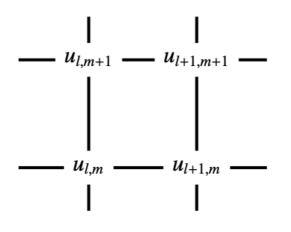
Consider a PE of the form
(1.15) where and is an irreducible multilinear polynomial. By putting the variable on the grid point of the integer lattice , the PE (1.15) can be regarded as a relation on the quadrilateral given by
as shown in Figure 1.1. For this reason, a PE of the form (1.15) is called a quad-equation. Note that quad-equations are not necessarily autonomous but may contain parameters that evolve with or .
-
1.2. Plan of the paper
This paper is organized as follows. In §2, using the CABC property of the dKdV equation (1.1) and the lsG equation (1.2), we show that they have the CAC property. In §3, we show how the PEs (1.1) and (1.2) can be extended to systems of PEs on the 3-dimensional integer lattice. Some concluding remarks are given in §4. In Appendix A, we recall the definitions of the CAC and CABC properties. In Appendix B, we list the Lax pairs of the PEs (1.1) and (1.2) constructed in this study. In Appendix C, we give the proof of Theorem 3.3.
2. Consistencies of the dKdV equation and the lsG equation
In this section, we give the new consistencies of the dKdV equation (1.1) and the lsG equation (1.2). See Appendix A for descriptions of the CABC and CAC properties we deal with here.
2.1. A CABC-type BT from the PE (1.1) to the multi-quadratic equation (1.6)
The following system of equations is a new CABC-type BT from the PE (1.1) to Equation (1.6):
| (2.1a) | |||
| (2.1b) | |||
| (2.1c) | |||
where and . By direct calculation, we can verify that the system of equations (1.1) and (2.1) has the CABC and tetrahedron properties. Indeed, the following relations can be derived from the CABC-system (1.1) and (2.1):
| (2.2) |
As shown in [11, 15], the Lax pair (B.1) with (B.2a) of the PE (1.1) can be constructed from the equations (2.1b) and (2.1c) by setting
| (2.3) |
2.2. A CAC-type BT from the PE (1.1) to the PE (1.2) (I)
In this subsection, using the CABC-type BTs (1.5) and (1.7), we obtain a CAC-type BT from the PE (1.1) to the PE (1.2).
Eliminating from the equations (1.5b) and (1.7b), we obtain
| (2.4) |
Let us assume that the following holds:
| (2.5) |
which satisfies Equation (2.4). Eliminating from Equation (1.5b) by using Equation (2.5) and from Equation (1.5c) by using Equation (2.5)m→m+1, we obtain
| (2.6a) | |||
| (2.6b) | |||
respectively. The equations above, together with the PEs (1.1) and (1.2), lead to the following theorem.
Theorem 2.1.
The following system has the CAC property but does not have the tetrahedron property:
| (2.7a) | |||
| (2.7b) | |||
| (2.7c) | |||
| (2.7d) | |||
where and are given by Equation (1.8). Since the equations (2.7a) and (2.7d) are equal to the PEs (1.1) and (1.2), respectively, we can also say that the pair of equations (2.7b) and (2.7c) is a CAC-type BT from the PE (1.1) to the PE (1.2).
Proof.
Theorem 2.1 gives the following corollary.
Remark 2.3.
2.3. A CAC-type BT from the PE (1.1) to the PE (1.2) (II)
In this subsection, using the CABC-type BTs (1.7) and (2.1), we obtain a CAC-type BT from the PE (1.1) to the PE (1.2). Since the process for demonstrating the result is the same as that for the CABC-type BTs (1.5) and (1.7) discussed in §2.2, we omit detailed arguments.
Theorem 2.5.
The following system has the CAC property but does not have the tetrahedron property:
| (2.12a) | |||
| (2.12b) | |||
| (2.12c) | |||
| (2.12d) | |||
where and are given by Equation (1.8). Since the equations (2.12a) and (2.12d) are equal to the PEs (1.1) and (1.2), respectively, we can also say that the pair of equations (2.12b) and (2.12c) is a CAC-type BT from the PE (1.1) to the PE (1.2).
Proof.
2.4. A CAC-type auto-BT of the PE (1.2)
In this subsection, using two CAC-systems (2.7) and (2.12), we obtain a CAC-system, which implies a CAC-type auto-BT of the PE (1.2).
Here, let us use the following CAC-system:
| (2.16a) | |||
| (2.16b) | |||
| (2.16c) | |||
| (2.16d) | |||
where and
| (2.17) |
instead of the CAC-system (2.7) with the variable and the parameters , in the system (2.7) replaced by the variable and the parameters , , respectively. Eliminating from the equations (2.12b) and (2.16b) and from the equations (2.12c) and (2.16c), we obtain
| (2.18a) | |||
| (2.18b) | |||
respectively. The equations above, together with the equations (2.12d) and (2.16d), lead to the following theorem.
Theorem 2.7.
The following system has the CAC property but does not have the tetrahedron property:
| (2.19a) | |||
| (2.19b) | |||
| (2.19c) | |||
| (2.19d) | |||
where
| (2.20) |
Since both of the equations (2.19a) and (2.19d) are equal to the PE (1.2), we can also say that the pair of equations (2.19b) and (2.19c) is a CAC-type auto-BT of the PE (1.2).
Proof.
Consider the cube in Figure 2.2. In the three different ways (see Appendix A.1), can be uniquely represented by the initial values as
| (2.21) |
Since depends on , the tetrahedron property does not hold. Moreover, the condition (2.20) can be obtained from the conditions (1.8) and (2.17). Therefore, we have completed the proof. ∎
Setting
| (2.22) |
from the equations (2.19b) and (2.19c), we obtain the Lax pair (B.4) of the PE (1.2).
Remark 2.8.
3. Integrable systems on the 3-dimensional integer lattice
In general, if a quad-equation has a CAC-type auto-BT, it can be easily extended to a system of PEs on the 3-dimensional integer lattice . (See [1, 9, 20].) However, in the case of non-auto-BTs, a little ingenuity is required. (See [4].) In this section, we show how quad-equations that have CABC-type BTs, which are non-auto-BTs, can be extended to a system of PEs on the lattice . Moreover, we also show how the resulting system can be reduced to systems on the lattice associated with the CAC-type BTs.
3.1. A system of PEs on the lattice associated with the CABC property
In this subsection, using the three CABC-systems (1.5), (1.7) and (2.1), we construct an integrable system of PEs on the lattice . We also show the -function of the resulting system.
Remark 3.1.
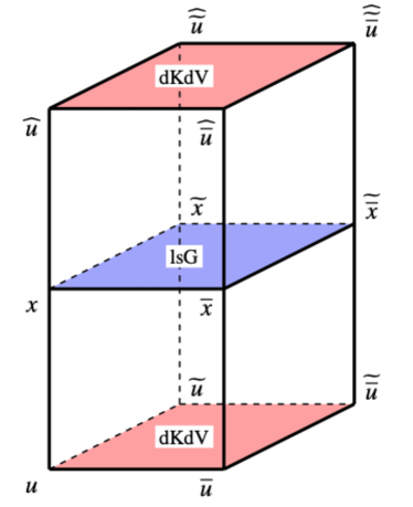
Let us denote the cubes for the three CABC-systems (1.5), (1.7) and (2.1) by the symbols , and , respectively. (See §A.2 for the correspondence between a CABC-system and a cube.) Overlap the cubes as in Figure 3.1 (Left), in the order , , , , so that the facing surfaces have the same equations. We here also denote the resulting rectangular constructed by the set of four stacked cubes by the symbol . Because both of the face-equations at the bottom and top of are the dKdV equation, it can be placed repeatedly up and down as shown in Figure 3.1 (Right). Note that since the parameter is not included in the dKdV equation, a different can be chosen for each stack of . This repeated placement yields the following system of PEs on the lattice :
| (3.1a) | |||
| (3.1b) | |||
| (3.1c) | |||
| (3.1d) | |||
| (3.1e) | |||
| (3.1f) | |||
| (3.1g) | |||
| (3.1h) | |||
where , , and
| (3.2) |
Remark 3.2.
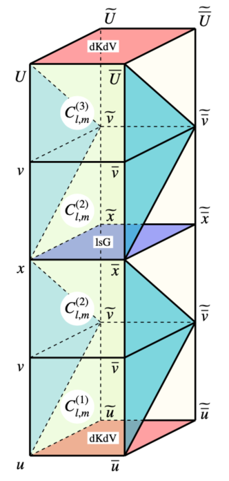
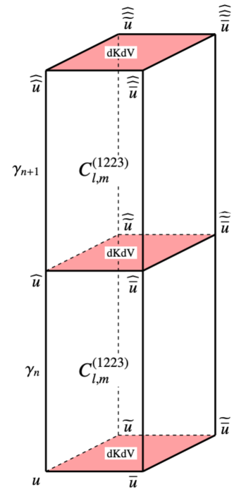
(Right): Two rectangulars . Since we choose a different parameter for each , we place the parameters on the vertical line segments of the rectangles.
The -function is one of the most important objects in the theory of integrable systems. We show the -function of the system (3.1) in the following theorem.
Theorem 3.3.
Let be the solution of the following bilinear equations:
| (3.3a) | |||
| (3.3b) | |||
Then, the -function of the system (3.1) is given as
| (3.4) |
Proof.
The proof is given in Appendix C. ∎
3.2. Systems of PEs on the lattice associated with the CAC property
In this subsection, we derive integrable systems on the lattice associated with the CAC property from the system (3.1).
As in §2.2 and §2.3, eliminating the -variable from the system (3.1) we obtain the following system of PEs depending only on the - and -variables:
| (3.5a) | |||
| (3.5b) | |||
| (3.5c) | |||
| (3.5d) | |||
| (3.5e) | |||
| (3.5f) | |||
Indeed, eliminating from the equations (3.1c) and (3.1e), we obtain
| (3.6) |
Then, eliminating -variable from the equations (3.1c) and (3.1d) by using the equation above, we obtain the equations (3.5c) and (3.5d), respectively. Moreover, eliminating from the equations (3.1e) and (3.1g), we obtain
| (3.7) |
and then eliminating -variable from the equations (3.1g) and (3.1h) by using the equation above, we obtain the equations (3.5e) and (3.5f), respectively.
Remark 3.4.
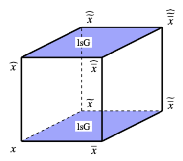
(Right): A cube for the CAC-system (3.8).
As in §2.4, we eliminate from the equations (3.5c)n→n+1 and (3.5e). Also, we eliminate from the equations (3.5d)n→n+1 and (3.5f). The resulting equations, together with Equation (3.5b), lead to the following system of PEs depending only on the -variable:
| (3.8a) | |||
| (3.8b) | |||
| (3.8c) | |||
Remark 3.5.
-
Both equations (3.8b) and (3.8c) are also the lsG equation. Indeed, by setting
(3.9) Equation (3.8b) can be rewritten as the following standard form of the lsG equation in -direction:
(3.10) while by setting
(3.11) Equation (3.8c) can also be rewritten as the following standard form of the lsG equation in -direction:
(3.12)
4. Concluding remarks
In this paper, using the CABC properties of the dKdV equation (1.1) and the lsG equation (1.2), we have shown that they have the CAC property. Using the CABC and CAC properties, we also obtained their new Lax pairs. Moreover, we have constructed the integrable system (3.1) on the lattice by stacking the cubes associated with the CABC property in the third direction and have clarified the structure of its -function.
In addition to the dKdV and lsG equations, there exist other integrable PEs for which we still do not know whether they have the CAC property. We have shown that it is useful to consider the CABC property to clarify the CAC property of PEs. Many studies have been done to find PEs which have the CAC property (see §1). However, the dKdV and lsG equations have the CAC property but are not included in these previous studies. For the reasons above, classifying PEs with the CABC property may be important for clarifying the CAC property of known integrable PEs. Moreover, it may lead to finding new integrable PEs. This should be a subject of future research.
Acknowledgment
The author would like to thank Dr. Pavlos Kassotakis and Dr. Yang Shi for fruitful discussions. This research was supported by a JSPS KAKENHI Grant Number JP19K14559. The author used Wolfram Mathematica for checking computations.
Appendix A The CAC and CABC properties
In this appendix, we explain the consistency around a cube (CAC) property of a system of PEs in a particular form. In addition, we also explain the consistency around a broken cube (CABC) property of a system of PEs in a particular form. For more general definitions, see [3, 9, 16, 24] for the CAC property and see [11, 15] for the CABC property.
Remark A.1.
For simplicity, we omit the parameters of the equations in this appendix. Moreover, the equations in this appendix are not limited to autonomous type. For example, the relation between and is not simple replacement of the corresponding -variables; applying to gives . See §2 for examples involving parameters.
A.1. The CAC property
Let us consider the following system of PEs:
| (A.1a) | |||
| (A.1b) | |||
| (A.1c) | |||
| (A.1d) | |||
where and . Here, the functions , , and are irreducible multilinear polynomials in four variables. Consider the following sublattice of the lattice :
| (A.2) |
and assign the - and -variables on the vertices of the sublattice by the following correspondences:
| (A.3) |
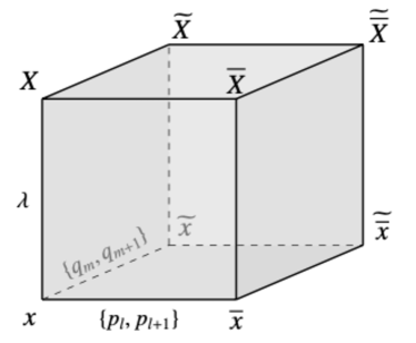
Then, focusing on the cube given by the 8 points
| (A.4) |
from the system (A.1), we obtain the following face-equations of the cube (see Figure A.1):
| (A.5a) | |||
| (A.5b) | |||
| (A.5c) | |||
| (A.5d) | |||
| (A.5e) | |||
| (A.5f) | |||
The CAC and tetrahedron properties are defined as follows.
-
We say that the PE (A.1a) (or the PE (A.1d)) has the CAC property if the system (A.1) has the CAC property. The pair of equations (A.1b) and (A.1c) is then referred to as a CAC-type BT from the PE (A.1a) to the PE (A.1d) (or from the PE (A.1d) to the PE (A.1a)). When the equations (A.1a) and (A.1d) are the same PE, the CAC-type BT (A.1b) and (A.1c) is specifically called a CAC-type auto-BT of the PE (A.1a).
Remark A.2.
Even if Equation (A.1a) has the CAC property, it is not necessarily integrable[8]. Even if a Lax pair of Equation (A.1a) is constructed from the CAC-type BT (A.1b) and (A.1c) by the method in [3, 9, 16, 24], it may be fake [6] or weak [10]. From this perspective, in [8], the CAC-type BT (A.1b) and (A.1c) are characterized as follows. Calculate in the following two ways.
- (a)
- (b)
If is automatically equal, then the CAC-type BT (A.1b) and (A.1c) is said to be trivial. If only Equation (A.5a) is obtained from , then the CAC-type BT (A.1b) and (A.1c) is said to be strong. If yields Equation (A.5a) plus other PEs for , then the CAC-type BT (A.1b) and (A.1c) is said to be weak. A trivial BT gives a fake Lax pair, and a weak BT gives a weak Lax pair. It is claimed in [8] that if the CAC-type BT is strong, then the integrability of (A.1a) should be guaranteed.
A.2. The CABC property
Let us consider the following system of PEs:
| (A.6a) | |||
| (A.6b) | |||
| (A.6c) | |||
| (A.6d) | |||
where and . Here, the functions , and are irreducible multilinear polynomials in four variables. The function is a polynomial in three variables satisfying the following:
-
1)
, ;
-
2)
Let be the solution of . Then, is a rational function that depends on and , that is, the following hold:
(A.7)
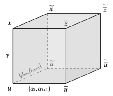
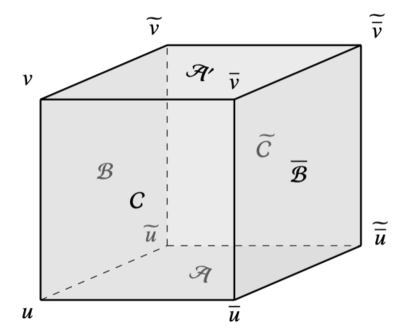
Assign the - and -variables on the sublattice (A.2) by the correspondence (A.3). Then, by considering the cube consisting of the eight vertices (A.4) (see Figure A.2), the system of equations around the cube obtained from the system (A.6) is the following:
| (A.8a) | |||
| (A.8b) | |||
| (A.8c) | |||
| (A.8d) | |||
| (A.8e) | |||
| (A.8f) | |||
The CABC and tetrahedron properties are defined as follows.
-
There are following three ways to calculate by using all the equations in the system (A.8) with as initial values.
- (a)
- (b)
- (c)
When is uniquely determined as a rational function with the initial values , then the system (A.6) is said to have the CABC property or said to be a CABC-system; the PE (A.6a) is said to have the CABC property.
Appendix B Lax pairs of the dKdV equation and the lsG equation
In this appendix, we show Lax pairs of the dKdV equation (1.1) and the lsG equation (1.2) obtained in this study.
B.1. Lax pairs of the PE (1.1)
B.2. A Lax pair of the PE (1.2)
Appendix C Proof of Theorem 3.3
Define by
| (C.1) |
where is a function satisfying the bilinear equations (3.3). Then, using Equation (3.4), we can express the variables , and in the -variable as
| (C.2a) | |||
| (C.2b) | |||
| (C.2c) | |||
Note that we use Equation (3.3b) for the deformation in Equation (C.2a). Moreover, the following lemma holds.
Lemma C.1.
The following relations hold:
| (C.3a) | |||
| (C.3b) | |||
Proof.
Consider the system (3.1) expressed in the -variable by using the equations (C.2). It is sufficient to show that the system (3.1) expressed in the -variable can be solved by the equations (C.3). For simplicity, we omit the description of the specific equations written in the -variable and itemize the method below by using only words.
- •
- •
- •
- •
Therefore, we have completed the proof of Theorem 3.3.
References
- [1] V. E. Adler, A. I. Bobenko, and Y. B. Suris. Classification of integrable equations on quad-graphs. The consistency approach. Comm. Math. Phys., 233(3):513–543, 2003.
- [2] V. E. Adler, A. I. Bobenko, and Y. B. Suris. Discrete nonlinear hyperbolic equations: classification of integrable cases. Funktsional. Anal. i Prilozhen., 43(1):3–21, 2009.
- [3] A. I. Bobenko and Y. B. Suris. Integrable systems on quad-graphs. Int. Math. Res. Not. IMRN, (11):573–611, 2002.
- [4] R. Boll. Classification of 3D consistent quad-equations. J. Nonlinear Math. Phys., 18(3):337–365, 2011.
- [5] R. Boll. Corrigendum: Classification of 3D consistent quad-equations. J. Nonlinear Math. Phys., 19(4):1292001, 3, 2012.
- [6] S. Butler and M. Hay. Two definitions of fake Lax pairs. In AIP Conference Proceedings, volume 1648, page 180006. AIP Publishing LLC, 2015.
- [7] H. W. Capel, F. W. Nijhoff, and V. G. Papageorgiou. Complete integrability of Lagrangian mappings and lattices of KdV type. Phys. Lett. A, 155(6-7):377–387, 1991.
- [8] J. Hietarinta. Search for CAC-integrable homogeneous quadratic triplets of quad equations and their classification by BT and Lax. J. Nonlinear Math. Phys., 26(3):358–389, 2019.
- [9] J. Hietarinta, N. Joshi, and F. W. Nijhoff. Discrete systems and integrability. Cambridge Texts in Applied Mathematics. Cambridge University Press, Cambridge, 2016.
- [10] J. Hietarinta and C. Viallet. Weak Lax pairs for lattice equations. Nonlinearity, 25(7):1955–1966, 2012.
- [11] N. Joshi and N. Nakazono. On the three-dimensional consistency of Hirota’s discrete Korteweg-de Vries equation. Stud. Appl. Math., 147(4):1409–1424, 2021.
- [12] K. Kajiwara and Y. Ohta. Bilinearization and Casorati determinant solution to the non-autonomous discrete KdV equation. Journal of the Physical Society of Japan, 77(5):054004, 2008.
- [13] P. Kassotakis and M. Nieszporski. Difference systems in bond and face variables and non-potential versions of discrete integrable systems. J. Phys. A, Math. Theor., 51(38):21, 2018. Id/No 385203.
- [14] D. J. Korteweg and G. De Vries. On the change of form of long waves advancing in a rectangular canal, and on a new type of long stationary waves. Phil. Mag. (5), 39:422–443, 1895.
- [15] N. Nakazono. Properties of the non-autonomous lattice sine-Gordon equation: consistency around a broken cube property. SIGMA. Symmetry, Integrability and Geometry: Methods and Applications, 18:032, 2022.
- [16] F. W. Nijhoff. Lax pair for the Adler (lattice Krichever-Novikov) system. Phys. Lett. A, 297(1-2):49–58, 2002.
- [17] F. W. Nijhoff and H. W. Capel. The discrete Korteweg-de Vries equation. Acta Appl. Math., 39(1-3):133–158, 1995. KdV ’95 (Amsterdam, 1995).
- [18] F. W. Nijhoff, H. W. Capel, G. L. Wiersma, and G. R. W. Quispel. Bäcklund transformations and three-dimensional lattice equations. Phys. Lett. A, 105(6):267–272, 1984.
- [19] F. W. Nijhoff, G. R. W. Quispel, and H. W. Capel. Direct linearization of nonlinear difference-difference equations. Phys. Lett. A, 97(4):125–128, 1983.
- [20] F. W. Nijhoff and A. J. Walker. The discrete and continuous Painlevé VI hierarchy and the Garnier systems. Glasg. Math. J., 43A:109–123, 2001. Integrable systems: linear and nonlinear dynamics (Islay, 1999).
- [21] J. J. C. Nimmo and W. K. Schief. An integrable discretization of a -dimensional sine-Gordon equation. Stud. Appl. Math., 100(3):295–309, 1998.
- [22] G. R. W. Quispel, F. W. Nijhoff, H. W. Capel, and J. van der Linden. Linear integral equations and nonlinear difference-difference equations. Phys. A, 125(2-3):344–380, 1984.
- [23] S. Tremblay, B. Grammaticos, and A. Ramani. Integrable lattice equations and their growth properties. Phys. Lett., A, 278(6):319–324, 2001.
- [24] A. Walker. Similarity reductions and integrable lattice equations. Ph.D. Thesis, University of Leeds, 2001.