Consistent Estimation of Low-Dimensional Latent Structure
in High-Dimensional Data
Abstract
We consider the problem of extracting a low-dimensional, linear latent variable structure from high-dimensional random variables. Specifically, we show that under mild conditions and when this structure manifests itself as a linear space that spans the conditional means, it is possible to consistently recover the structure using only information up to the second moments of these random variables. This finding, specialized to one-parameter exponential families whose variance function is quadratic in their means, allows for the derivation of an explicit estimator of such latent structure. This approach serves as a latent variable model estimator and as a tool for dimension reduction for a high-dimensional matrix of data composed of many related variables. Our theoretical results are verified by simulation studies and an application to genomic data.
Keywords: exponential family distribution, factor analysis, high-dimensional data, latent variable model, spectral decomposition
1 Introduction
Low-dimensional latent variable models are often used to capture systematic structure in the conditional mean space of high-dimensional random variables (rv’s). This has been a popular strategy in high-dimensional probabilistic modeling and data analysis, and it serves as an attractive strategy for dimension reduction and recovering latent structure. Examples include factor analysis (Bartholomew et al., 2011), probabilistic principal components analysis (PCA) (Tipping and Bishop, 1999), non-negative matrix factorization (Lee and Seung, 1999), asymptotic PCA (Leek, 2011), latent Dirichlet allocation (LDA) (Blei et al., 2003), and exponential family distribution extensions of PCA (Collins et al., 2001).
Let be an observed data matrix of variables (one variable per row), each with observations, whose entries are rv’s such that
| (1) |
where is the expectation operator, is a matrix of latent variables, and is a matrix of coefficients relating the latent variables to the observed variables. Furthermore, the dimensions are such as . In model (1), the conditional mean of for a fixed only depends on the th column of , and each row of the conditional mean matrix lies in the row space of . The latent structure in is therefore induced by .
The above model is a general form of several highly used models. This includes instances of factor analysis (Bartholomew et al., 2011), probabilistic PCA (Tipping and Bishop, 1999), mixed membership clustering in population genetics (Pritchard et al., 2000; Alexander et al., 2009) which is closely related to LDA, and non-negative matrix factorization (Lee and Seung, 1999). Whereas the specialized models are often focused on the probabilistic interpretation of the columns of , we are instead here interested in its row space, . This row space is sufficient for: (i) characterizing systematic patterns of variation in the data , which can be used for exploratory data analysis or dimension reduction; (ii) accounting for the latent variables in downstream modeling of (Leek and Storey, 2007, 2008) that requires adjustment for these variables; (iii) potentially identifying suitable initial values or geometric constraints for algorithms that estimate probabilistically constrained versions of ; (iv) or recovering itself if additional geometric properties are known (e.g., as in Arora et al. (2013)). Furthermore, many of the above models make assumptions about the probability distribution of that may be untrue on a given data set. One can compare our estimate of (which makes minimal assumptions) to the space induced by the model-based estimates of to gauge the accuracy of the model assumptions and fit. Therefore, we focus on estimation of the latent variable space . Estimation of may be tractable, but we do not focus on that here.
Leek (2011) and Anandkumar et al. (2012, 2015) have carried out work that is complementary to that presented here. They both study moment estimators of linear latent variable models applied to high-dimensional data. We explain how our work is related to Leek (2011) in Section 4.3 and how it is related to Anandkumar et al. (2012, 2015) in Section A. The strategies employed in these papers have ties to what we do here; however, they each consider different probabilistic models with theory that does not directly apply to the models we study.
We show that both the row space of (in Section 2) and the row rank of (in Section 3) can be consistently estimated using information from a suitably adjusted matrix . In Section 4, we specialize these general results to ’s that, conditional on , come from exponential family distributions. In particular, we explicitly construct a nonparametric, consistent estimator of the row space of for rv’s that follow the natural exponential family (NEF) with quadratic variance function (QVF) using information only up to their second moments, and the estimator is computationally straightforward to implement. In Section 5, we extend the results of previous sections to the case where is random. A simulation study is conducted in Section 6 to check and confirm our theoretical findings, and we apply the estimators to a genomics data set in Section 7. Finally, we end the article with a discussion in Section 8, collect in Section B all technical proofs, and present the the full set of results from simulation studies in Section C and Section D.
2 Almost Surely Estimating the Latent Linear Space
The big picture strategy we take is summarized as follows. Carrying out a decomposition related to Leek (2011), we first expand into four components:
| (2) | |||||
| (3) |
We then show the following about each of the components as , under the assumptions given in detail below:
-
•
: this term may be estimated arbitrarily well as by a diagonal matrix defined and studied below;
-
•
and : these terms converge to the zero matrix;
-
•
: this term converges to a symmetric matrix with positive eigenvalues whose leading eigenvectors span the row space of .
Once the convergence of these terms is rigorously established, the strategy we take is to form an estimate of term , denoted by , and show that the space spanned by the leading eigenvectors of converges to the row space of as . We then also provide a framework to estimate the dimension of the row space of and incorporate it into this estimation framework.
2.1 Model Assumptions
We first define the matrix norm for any real matrix and let denote a generic, finite constant whose value may vary at different occurrences. We first assume that is deterministic; the results in this section are extended to the case where is random in Section 5. The assumptions on model (1) are as follows:
- A1)
-
and is finite; are jointly independent with variance such that (which implies ), where is the variance operator.
- A2)
-
, where is the th row of . Further, for some and some non-negative sequence ,
(4)
Since we are considering model (1) for which is conditioned on , all random vectors in this model are by default conditioned on unless otherwise noted (e.g., Section 5). For conciseness we will omit stating “conditional on ” in this default setting.
We state a consequence of the assumption A2) as Lemma 1, whose proof is straightforward and omitted.
Lemma 1
If the assumption A2) holds, then
for each and .
The uniform boundedness results provided by Lemma 1 will be used to prove the convergence results later.
2.2 Asymptotically Preserves the Latent Linear Space
We first derive the asymptotic form of with the aid of the strong law of large numbers (SLLN) in Walk (2005). Let be the column-wise average variance of (where as defined above) and
| (5) |
the diagonal matrix composed of these average variances.
Theorem 2
Theorem 2 shows that becomes arbitrarily close to as the number of variables . In fact, it gives much more information on the eigensystem of (as we take the convention that an eigenvector always has norm ). Let be the eigenvalues of ordered into for (where here we take the convention that the ordering of the designated multiple copies of a multiple eigenvalue is arbitrary),
and be the eigenvalues of ordered into for .
Corollary 3
Under the assumptions for model (1),
| (7) |
Further, a.s. and
| (8) |
where denotes the linear space spanned by its arguments, and the symmetric set difference.
Corollary 3 reveals that asymptotically as the eigenvalues of converge to those of when both sets of eigenvalues are ordered the same way, that the dimension of the space spanned by all the eigenvectors corresponding to the largest eigenvalues of converges to as , and that is asymptotically spanned by the leading dimensional joint eigenspace induced by as . When the nonzero eigenvalues of are distinct, we easily have
| (9) |
where, modulo a sign, is the eigenvector corresponding to and that to .
When the dimension of the latent space and the diagonal matrix of the column-wise average variances are known, it follows by Corollary 3 that asymptotically spans the latent space , and converges to the row space with probability 1. However, in practice both and need to be estimated, which is the topic of the next three sections. Estimating the number of latent variables is in general a difficult problem. In our setting we also must accurately estimate , which can be a difficult task when the variances may all be different (i.e., heteroskedastic).
3 Consistently Estimating the Latent Linear Space Dimension
The strategy we take to consistently estimate the dimension of the latent variable space is to carefully scale the ordered eigenvalues of and identify the index of the eigenvalue whose magnitude separates the magnitudes of these eigenvalues into two particular groups when is large. Recall that, by Theorem 2 and Corollary 3, the difference between the vector of descendingly ordered eigenvalues of and that of those of converges to zero as . However, since and , we know that the largest eigenvalues of are positive but the rest are zero. This means that the largest eigenvalues of are all strictly positive as , while the smallest eigenvalues of converge to as . Depending on the speed of convergence of the smallest eigenvalues of to , if we suitably scale the eigenvalues of , then the scaled, ordered eigenvalues will eventually separate into two groups, those with very large magnitudes and the rest very small. The index of the scaled, ordered eigenvalues for which such a separation happens is then a consistent estimator of . If we replace with an estimator that satisfies a certain level of accuracy detailed below, then the previous reasoning applied to the eigenvalues of will also give a consistent estimator of .
To find the scaling sequence for the magnitudes of the eigenvalues of or equivalently the speed of convergence of the smallest eigenvalues of to , we define the matrix with entry , and study as a whole the random part of defined by
| (10) |
Note that the terms , and in correspond to those from equation (3). We will show that configured as a vector possesses asymptotic Normality after centering and scaling as . This then reveals that the scaling sequence for the eigenvalues of should be no smaller than being proportional to .
Let , and define
| (11) |
for , where and are respectively the th row of and the th column of . We have:
Proposition 4
With the concentration property of established by Proposition 4, we will be able to explore the possibility of consistently estimating by studying the magnitudes of eigenvalues of
| (12) |
where each is an estimate of for , and the ’s are ordered into for .
Theorem 5
Under the assumptions A1), A2) and A3), if
- A4)
-
for some non-negative such that ,
(13)
then
| (14) |
where is the probability measure and
| (15) |
Further, for any such that and , as ,
| (16) |
for any fixed . Therefore, letting
| (17) |
gives
| (18) |
where is the indicator of a set .
Theorem 5 shows that the speed of convergence, , of the eigenvalues of (and those of ) is essentially is determined by those related to and ; see equations (13)–(15). Further, it reveals that, when is known, with probability approaching to as , the scaled, ordered eigenvalues eventually separates into two groups: for all lie above but the rest all lie below for any chosen . In other words, for a chosen , the number of when is large is very likely equal to . However, in practice and are unknown, and even if they are known or can be estimated, unfortunately the hidden constants in (14) are unknown (even when ). Further, when is finite, the smallest eigenvalues of may not yet be identically zero, the hidden constants may have a large impact on estimating the scaling sequence , and rates slightly different than may have to be chosen to balance the effects of the hidden constants; see in Section 6 a brief discussion on the estimation of and the effects of choosing on estimating for finite .
Before we apply our theory to ’s that follow specific parametric distributions, we pause to comment on the key results obtained so far. Theorem 2 and Corollary 3 together ensure that asymptotically as we can span the row space of by the leading eigenvectors of (see the definition of in (5)). However, the conclusions in these results are based on a known and . In contrast, Proposition 4 and Theorem 5 retain similar assertions to those of Theorem 2 and Corollary 3 by replacing the unknown by its consistent estimate , and they enable us to construct a consistent estimate of such that the linear space spanned by the leading eigenvectors of consistently estimates as . This reveals that to consistently estimate in a fully data driven approach using our theory, it is crucial to develop a consistent estimate of .
4 Specializing to Exponential Family Distributions
We specialize the general results obtained in Section 2 and Section 3 for model (1) to the case when follow the single parameter exponential family probability density function (pdf) given by
| (19) |
where is the canonical link function, and and are known functions such that is a proper pdf. The values that can take are . The following corollary says that our general results on consistent estimation of the latent space and its dimension hold when the link function is bounded on the closure of the parameter space .
Corollary 6
We remark that the boundedness of on the closure of is not restrictive, in that in practice either is bounded in Euclidean norm or is bounded in supremum norm. The proof of Corollary 6 is a simple observation that is analytic in when (see, e.g. Letac and Mora, 1990) and that the derivative of in of any order is bounded when is bounded; the proof is thus omitted.
4.1 Estimating
With Corollary 6 (see also the discussion at the end of Section 3), we only need to estimate (which in turn yields ) in order to consistently estimate and . To obtain an estimate of when potentially all are different from each other (i.e., complete heteroskedasticity), we exploit the intrinsic relationship between and when come from a certain class of natural exponential family (NEF) distributions.
Lemma 7
| Normal | 1 | |||
|---|---|---|---|---|
| Poisson | ||||
| Binomial | ||||
| NegBin | ||||
| Gamma | ||||
| GHS |
Inspired by the availability of the function obtained in Lemma 7, we now state a general result on how to explicitly construct a that properly estimates .
Lemma 8
Let have pdf (19) such that for some function satisfying
| (22) |
Then
| (23) |
satisfies a.s. for each . If additionally, for each and some ,
| (24) |
then converges in distribution to a Normal random variable as .
Lemma 8 shows that in (12) with defined by (23) satisfies . Note that the first assertion in Lemma 8, i.e., a.s., clearly applies to that follow NEFs with QVF when their corresponding are in a set described in Corollary 6. We remark that requiring the closure of to be in the interior of is not restrictive, since in practice the ’s are not the boundary points of .
4.2 Simultaneously Consistently Estimating the Latent Linear Space and Its Dimension
We are ready to present a consistent estimator of the latent linear space :
- 1.
- 2.
-
3.
From the spectral decomposition where and , pick columns of corresponding to the largest .
-
4.
Set
(25) to be the estimate of . Note that can be regarded as an estimator of even though it is not our focus.
The above procedure is supported by the following theorem, whose proof is straightforward and omitted. More specifically, in (25) consistently estimates .
4.3 Normal Distribution with Unknown Variances
One of the exponential family distributions we considered above is . Suppose instead we assume that , where are unknown. Leek (2011) studies this important case, and obtains several results related to ours. Let be the ordered singular values resulting from the singular value decomposition (SVD) of . If we regress the top right singular vectors in this SVD from each row of , this yields total residual variation that is of proportion to the total variation in . In order to estimate , Leek (2011) employs the estimate
Using our notation, Leek (2011) then sets , where is the identity matrix, and proceeds to estimate based on as we have done. However, it must be the case that in order for to be well-behaved, so the assumptions and theory in Leek (2011) have several important differences from ours. We refer the reader to Leek (2011) for specific details on this important case. We note that taking our results together with those of Leek (2011), this covers a large proportion of the models utilized in practice.
5 Letting the Latent Variable Coefficients Be Random
We now discuss the case where is random but then conditioned. Assume that is a random matrix with entries defined on the probability space , and that the entries of , conditional on and , are defined on the probability space . Rather than model (1), consider the following model:
| (26) |
Suppose assumption A4) holds (see (13)) and:
- A1′)
-
and is finite; conditional on and , are jointly independent with variance such that (which implies ), where and are the expectation and variance wrt .
- A2′)
-
Either A2) holds -a.s., i.e., and
(27) or A2) holds in probability , i.e., as , and
(28) - A3′)
-
Conditional on , , and for any are all convergent -a.s. as .
Note that assumptions A1′), A2′) and A3′) are the probabilistic versions of assumptions A1), A2 and A3) that also account for the randomness of . Recall assumption A2) when is deterministic, i.e., for some and some non-negative sequence , . Assumption A2) implies that (see also Lemma 1):
| (29) |
These two uniform boundedness results in equation (29) are then used to show the a.s. convergence in Theorem 2 which induces the a.s. convergence in Corollary 3, the validity of Lindeberg’s condition as (34) that induces Proposition 4, convergence in probability in equations (14) and (16) that induces Theorem 5, Corollary 6, and Theorem 9.
Let be such that (27) does not hold, then . On the other hand, if (28) holds, then for any positive constants and there exists a such that the set
satisfies
whenever . Now if (27) holds, then the results on the a.s. convergence and on convergence in probability for remain true with respect to when is replaced by , as long as each is such that . In contrast, if (28) holds, then the results on the a.s. convergence for reduce to convergence in probability in . But those on convergence in probability for remain true with respect to when is replaced by , as long as each is with (where can be chosen to be small). Therefore, the results (except Lemmas 7 and 8) obtained in the previous sections hold with their corresponding probability statements, whenever, for some ,
| (30) |
holds a.s. or in probability in , and they allow to be random (and conditioned) or deterministic. Statistically speaking, an event with very small or zero probability is very unlikely to occur. This means that the practical utility of these results is not affected when (30) holds in the sense of (27) or (28) when is large.
6 A Simulation Study
We conducted a simulation study to demonstrate the validity of our theoretical results. The quality of is measured by
where is an estimate of , and . In fact, measures the difference between the orthogonal projections (as linear operators) induced by the rows of and those of respectively, and if and only if . We propose a rank estimator , directly applied to , based on Theorem 5. Specifically, for some positive and is used to scale the eigenvalues of , for which (dependent on ) is determined by a strategy of Hallin and Liska (2007) (that was also used by Leek, 2011); for more details, we refer the reader to these two references. We do so since the assertions in Theorem 5 are valid only for , assumption A3) may not be satisfied in our simulation study, and the unknown constants in equation (14) for the speed of convergence need to be estimated. However, we caution that, if the scaling sequence in Theorem 5 defined via (15) is not well estimated to capture the speed of convergence of the eigenvalues of , defined by (17) as an estimate of can be inaccurate; see our simulation study results.
6.1 Simulation Study Design
The settings for our simulation study are described below:
-
1.
We consider , and .
-
2.
The mean matrix and the observed data are generated within the following scenarios:
-
(a)
, , and .
-
(b)
, - with degrees of freedom and non-centrality , and .
-
(c)
with and . is such that for , for and , and otherwise.
-
(d)
with , , and .
-
(e)
with shape and mean , , and .
-
(a)
-
3.
For each combination of values in Step 1 and distributions in Step 2 above, the data matrix is generated independently times and then the relevant statistics are calculated.
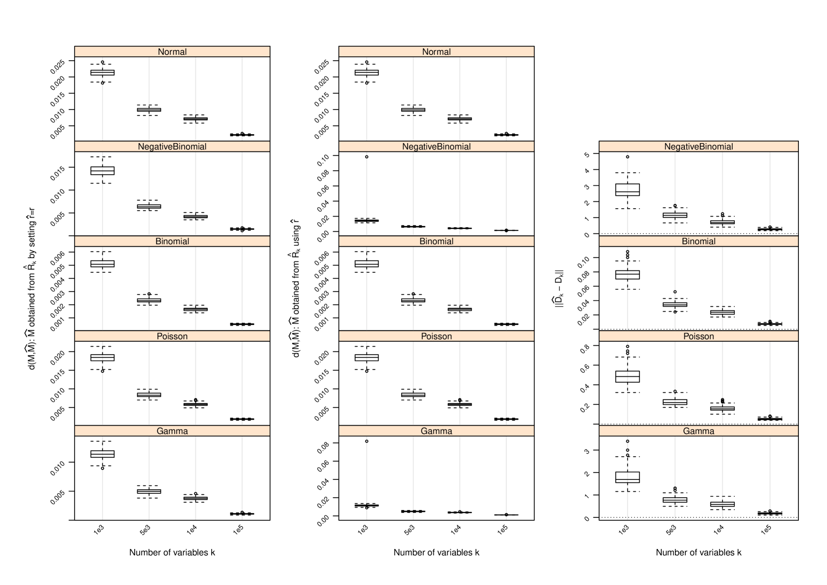
For each simulated data set, we measure the quality of by , that of by , and we record .
| Binomial | Gamma | NegBin | Normal | Poisson | |
|---|---|---|---|---|---|
| 1000 | 3 (97) | 24 (4) | 3 | 100 | 84 (6) |
| 5000 | 95 (5) | 30 (9) | 4 | 96 | 94 |
| 10,000 | 100 | 33 (22) | 27 (9) | 96 | 89 |
| 100,000 | 100 | 90 | 43 | 99 | 94 |
6.2 Simulation Study Results
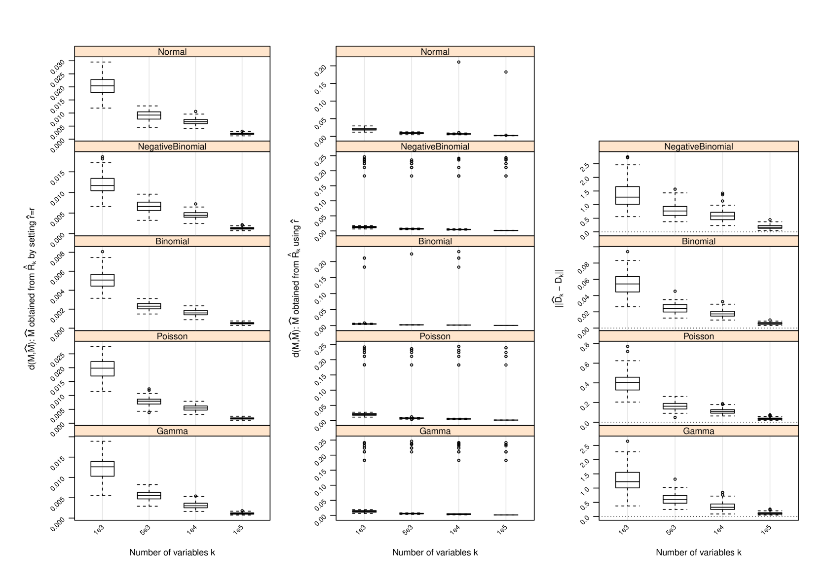
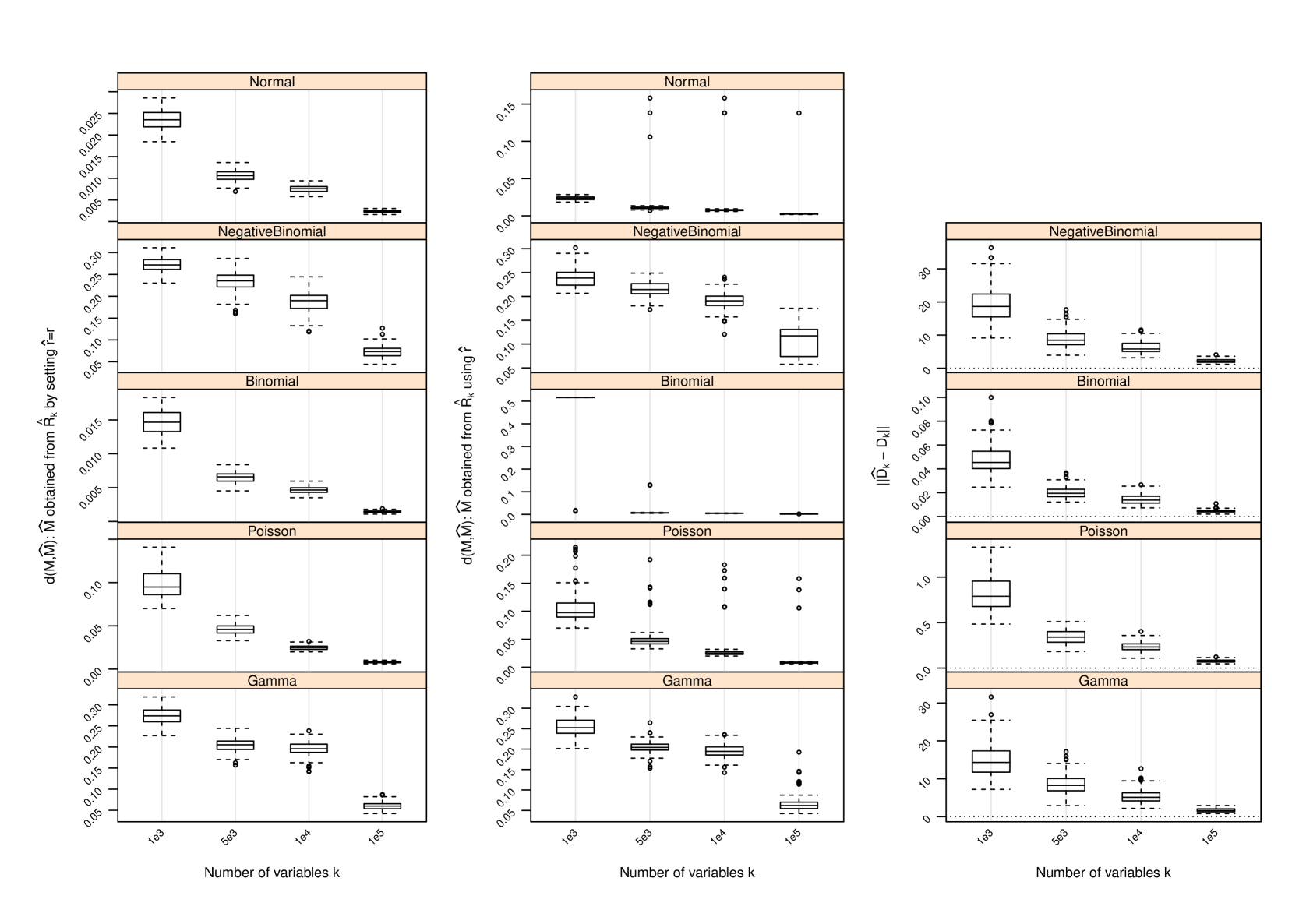
Figure 1 and Table 2 display the performance of the nonparametric estimator of , that of , and that of when and ; for other values of and , the performance of is provided in Section C and that of in Section D. The following conclusions can be drawn from the simulation study:
-
1.
with set as the true approximates with increasing accuracy as measured by the difference between their induced orthogonal projections when gets larger. In all settings, strong trends of convergence of to can be observed, even when is used. However, the speed of convergence can be slightly different for different settings due to the hidden constants in (4) and (14).
-
2.
As gets larger becomes more accurate, and strong trends of convergence of to can be observed in all settings. This is similar to the behavior of . However, the accuracy of in estimating does not seem to have a drastic impact on , since induces a shift by a diagonal matrix to the matrix and such a shift does not necessarily have a huge impact on the leading eigenvectors of and hence on . We do not report the performance of in the scenarios where since in this case and , and has been set.
-
3.
In all settings, can under- or over-estimate , and as increases becomes more accurate. However, when it does not reduce the accuracy of the estimate when is used to pick the number of leading eigenvectors of to estimate . In fact, when , additional linearly independent eigenvectors for may be used to span , giving better estimate than using the true . When , the accuracy of is reduced, since in this case the original row space can not be sufficiently spanned by . This is clearly seen from the plots on performance of .
-
4.
The scaling sequence plays a critical role on the accuracy of as an estimator of , since it decides where to “cut” the spectrum of for finite to give , where numerically all eigenvalues of are non-zero. In all settings, the non-adaptive choice of the sequence with has been used, and it can cause inaccurate scaling of the spectrum of and hence inaccurate estimate of . This explains why has been under-estimated when ’s follow Binomial distributions, and , since in these cases the magnitudes of the eigenvalues of have more complicated behavior, and are too large compared the magnitudes of these eigenvalues; see Tables S1–S3 in Section C for results when and those when . We found that when follow Binomial distributions in the simulation study, in order to accurately estimate , should be set for and that should be set for . The non-adaptive choice of also explains why over-estimates when ’s follow the Negative Binomial distributions or gamma distributions in the simulation study, since these two types of distributions are more likely to generate outliers that counterbalance the speed of concentration as gets larger, and affect the separation of the spectrum of the limiting matrix . In other words, for these two cases, are too small in magnitudes in order to scale up the spectrum of to the point of separation in order to estimate . In general, the magnitude of plays a role in the asymptotic property of as , and it affects the speed of convergence of through the hidden constants in (14) even when all needed assumptions are satisfied for Theorem 5. This explains why larger does not necessarily induce more accurate when increases but does not increase at a compatible speed when is finite; see Tables S1–S3 in Section C. However, deciding the hidden constants in (14) is usually very hard, and accurately estimating , being also the number of factors in factor models, is in general a very challenging problem.
7 Application to an RNA-Seq Study
In Robinson et al. (2015), we measured genome-wide gene expression in the budding yeast Saccharomyces cerevisiae in a nested factorial experimental design that allowed us to carefully partition gene expression variation due to both biology and technology. The technology utilized to measure gene expression is called “RNA-seq”, short for RNA sequencing. This technology provides a digital measure of gene expression in that mRNA molecules are discretely sequenced and therefore counted (Wang et al., 2009). The resulting matrix of RNA-seq counts represents gene expression measurements on 6575 genes across 16 samples. We also have a design matrix of dimension that captures the experimental design and apportionment of variation throughout the data. The data here are counts, and RNA-seq count data are typically modeled as overdispersed Poisson data (McCarthy et al., 2012). It can be verified on these data that, because of the experimental design, there is very little over-dispersion once the experimental design is taken into account; we therefore utilize the Poisson distribution in this analysis.
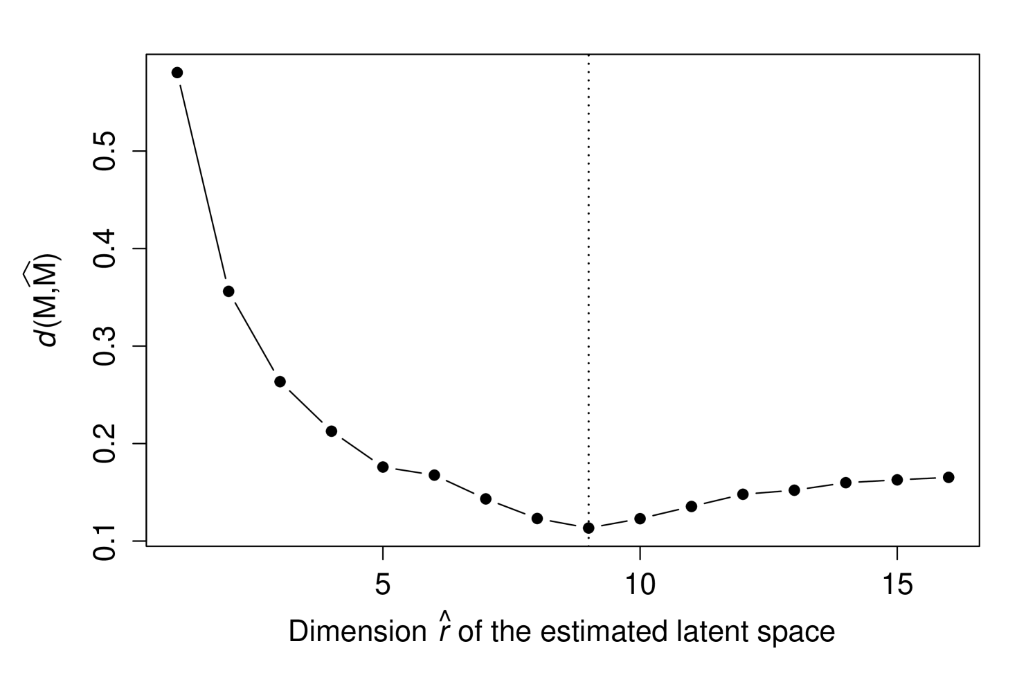
We set to be the matrix of RNA-seq counts and the design matrix, where each row of is normalized to have unit Euclidean norm. Ignoring our knowledge of , we applied the proposed estimator using the Poisson distribution formula to yield an estimate over a range of values of . In evaluating , we utilized the measure defined in Section 6.
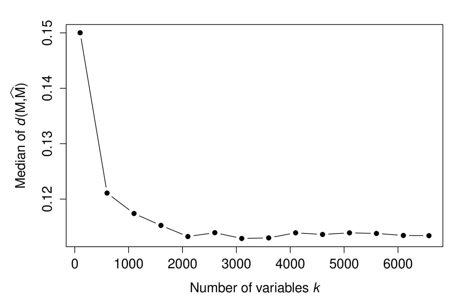
Figure 2 shows how changes with the dimension of . It can be seen that the minimum value is at (where is the true dimension of ). We then randomly sampled rows of to quantify how changes as the number of variables grows. Figure 3 shows the median values over 50 random samplings for each value, where a convergence with respect to can be observed. In summary, this analysis shows that the proposed methodology is capable of accurately capturing the linear latent variable space on real data that is extremely heteroskedastic and does not follow the Normal distribution.
8 Discussion
We have proposed a general method to consistently estimate the low-dimensional, linear latent variable structure in a set of high-dimensional rv’s. Further, by exploiting the intrinsic relationship between the moments of natural exponential family (NEF) distributions that have quadratic variance functions (QVFs), we are able to explicitly recover this latent structure by using just the second moments of the rv’s even when these rv’s have heteroskedastic variances. Empirical evidence confirms our theoretical findings and the utility of our methodology. Once the latent structure has been well estimated, the variable-specific coefficients of the latent variables can be estimated via appropriate estimation methods.
We point out that, under the same assumptions A1), A2), A3) and A4), the theoretical results in Sections 2, 3 and 4 hold for the unconditional model
| (31) |
when both and are deterministic with . In this case the conditional distribution of each given in model (1), i.e., when is a realization of a random matrix , becomes the marginal distribution of in model (31) and the proofs proceed almost verbatim as those for model (1). Further, for the model
| (32) |
when is random but is deterministic with , under the assumptions A1′), A2′), A3′) and A4), similar arguments as those given in Section 5 imply that the theoretical results obtained in Sections 2, 3 and 4 hold when the probabilistic statements in the conclusions there are adjusted in the way detailed in Section 5.
We have observed that for certain NEF distribution configurations, estimating the rank of the linear space generated by the latent structure can can be challenging, even with the theory we provided, if the scaling sequence to separate the limiting spectrum of the adjusted gram matrix of the data is not adaptively specified. The need for choosing an adaptive scaling sequence comes from the hidden constants that describe the asymptotic speed of convergence, and it can be a delicate task to do so in non-asymptotic settings. This is reflective of the more general challenge of estimating the dimension of a latent variable model.
Finally, we briefly point out that, when the have pdf such that
form an exponential dispersion family (see, e.g., Jørgensen, 1987), an explicit estimator of (and hence that of ) will require results beyond those provided in this work, even if the unknown dispersion parameter is constant. We leave this case to future research.
Acknowledgements
This research is funded by the Office of Naval Research grant N00014-12-1-0764 and NIH grant HG002913.
References
- Alexander et al. (2009) D. H Alexander, J Novembre, and K Lange. Fast model-based estimation of ancestry in unrelated individuals. Genome Research, 19(9):1655–1664, 2009.
- Anandkumar et al. (2012) Anima Anandkumar, Dean P. Foster, Daniel Hsu, Sham M. Kakade, and Yi-Kai Liu. A spectral algorithm for latent Dirichlet allocation. Advances in Neural Information Processing Systems, 25, 2012.
- Anandkumar et al. (2015) Anima Anandkumar, Dean P. Foster, Daniel Hsu, Sham M. Kakade, and Yi-Kai Liu. A spectral algorithm for latent Dirichlet allocation. Algorithmica, 72:193 C–214, 2015.
- Arora et al. (2013) Sanjeev Arora, Rong Ge, Yonatan Halpern, David Mimno, Ankur Moitra, David Sontag, Yichen Wu, and Michael Zhu. A practical algorithm for topic modeling with provable guarantees. In Proceedings of The 30th International Conference on Machine Learning, pages 280–288, 2013.
- Bartholomew et al. (2011) D. J. Bartholomew, M. Knott, and I. Moustaki. Latent Variable Models and Factor Analysis: A Unified Approach. Wiley Series in Probability and Statistics, 3rd edition, 2011.
- Blei et al. (2003) David M. Blei, Andrew Ng, and Michael Jordan. Latent dirichlet allocation. JMLR, 3:993–1022, 2003.
- Collins et al. (2001) Michael Collins, Sanjoy Dasgupta, and Robert E Schapire. A generalization of principal components analysis to the exponential family. In Advances in neural information processing systems, pages 617–624, 2001.
- Hallin and Liska (2007) Marc Hallin and Roman Liska. Determining the number of factors in the general dynamic factor model. J. Amer. Statist. Assoc., 102(478):603 C617, 2007.
- Hoffman and Wielandt (1953) A.J. Hoffman and H.W. Wielandt. The variation of the spectrum of a normal matrix. Duke Math. J., 20(1):37–39, 1953.
- Jørgensen (1987) Bent Jørgensen. Exponential dispersion models. J. R. Statist. Soc. B, 49(2):127–162, 1987.
- Lee and Seung (1999) D. D. Lee and S. Seung. Learning the parts of objects by non-negative matrix factorization. Nature, 401:788–791, 1999.
- Leek (2011) Jeffrey T. Leek. Asymptotic conditional singular value decomposition for high-dimensional genomic data. Biometric, 67(2):344–352, 2011.
- Leek and Storey (2007) Jeffrey T Leek and John D Storey. Capturing heterogeneity in gene expression studies by surrogate variable analysis. PLoS Genet, 3(9):e161, 2007.
- Leek and Storey (2008) Jeffrey T. Leek and John D. Storey. A general framework for multiple testing dependence. Proc. Natl. Acad. Sci. U.S.A., 105(48):18718–18723, 2008.
- Letac and Mora (1990) Gerard Letac and Marianne Mora. Natural real exponential families with cubic variance functions. Ann. Statist., 18(1):1–37, 1990.
- McCarthy et al. (2012) Davis J McCarthy, Yunshun Chen, and Gordon K Smyth. Differential expression analysis of multifactor RNA-Seq experiments with respect to biological variation. Nucleic Acids Research, 40(10):4288–4297, 2012.
- Morris (1982) Carl N. Morris. Natural exponential families with quadratic variance functions. Ann. Statist., 10(1):65–80, 1982.
- Pritchard et al. (2000) J. K. Pritchard, M. Stephens, and P. Donnelly. Inference of population structure using multilocus genotype data. Genetics, 155(2):945–959, 2000.
- Robinson et al. (2015) David G. Robinson, Jean Y. Wang, and John D. Storey. A nested parallel experiment demonstrates differences in intensity-dependence between rna-seq and microarrays. Nucleic acids research, 2015. doi: 10.1093/nar/gkv636.
- Tipping and Bishop (1999) Michael E. Tipping and Christopher M. Bishop. Probabilistic principal component analysis. Journal of the Royal Statistical Society: Series B, 61(3):611–622, 1999. doi: 10.1111/1467-9868.00196.
- Van der Vaart (1998) A. W. Van der Vaart. Asymptotic Statistics. Cambridge Univ. Press, 1998.
- Walk (2005) Harro Walk. Strong laws of large numbers by elementary Tauberian arguments. Monatsh. Math., 144(4):329–346, 2005.
- Wang et al. (2009) H. S. Wang, B. Li, and C. L. Leng. Shrinkage tuning parameter selection with a diverging number of parameters. Journal of the Royal Statistical Society Series B-Statistical Methodology, 71:671–683, 2009.
A Relationship to Anandkumar et al.
Anandkumar et al. (2012, 2015) consider a different class of probabilistic models than we consider. We establish this by rewriting their model in our notation. We consider the model
where is a matrix of observations on variables. The data points can take on a wide range of classes of variables, from Binomial outcomes, to count data, to continuous data (see Table 1, for example). Variable can be written as , which is a vector. In terms of this variable, our model assumes that
where is row of .
Anandkumar et al. (2012, 2015), on the other hand, assume that with the restriction that . This construction is meant to represent an observed document of text where there are words in the dictionary. They consider a single document with an infinite number of words. The vector tells us which of the words is present at location in the document. When they let , this means the number of words in the document grows to infinity.
The model studied in Anandkumar et al. (2012, 2015) is
where there are topics under consideration and the -vector gives the mixture of topics in this particular document. Each column of gives the multinomial probabilities of the words for the corresponding topic. Note that the linear latent variable model does not vary with , whereas in our model it does. Also, the dimensionality of the latent variable model is different than ours. Therefore, this is a different model than we consider.
Anandkumar et al. (2012, 2015) take the approach of calculating, projecting and decomposing the expectations of tensor products involving and , and then suggesting that these expectations can be almost surely estimated as by utilizing the analogous sample moments. In order to exactly recover modulo a permutation of its columns, additional assumptions are made by Anandkumar et al. (2012, 2015), such as knowledge of the sum of the unknown exponents in the Dirichlet distribution in the LDA model of Blei et al. (2003). It is also assumed that the number of topics is known.
B Proofs
Since we are considering the conditional model (1), i.e., , to maintain concise notations we introduce the conditional expectation and variance operators respectively as and . In the proofs, unless otherwise noted, the random vectors are conditioned on and the arguments for these random vectors are conditional on .
B.1 Proof of Theorem 2
Denote the terms in the order in which they appear in the expansion
as , and and , we see that by assumption (4). We claim that a.s. The entry of is , where for . Clearly, . Set . By Lemma 1, uniformly bounded th conditional moments of and Hölder’s inequality,
By independence conditional ,
Therefore, Theorem 1 of Walk (2005) implies that a.s., which validates the claim.
Consider the last term , whose th off-diagonal entry can be written as , where . Clearly, . The same reasoning as above implies
when . So, Theorem 1 of Walk (2005) implies that a.s. The diagonal entries of can be written as , where . Since and
it follows that
Hence, Theorem 1 of Walk (2005) implies a.s. and . Combining the limiting terms obtained above completes the proof.
B.2 Proof of Corollary 3
We show (7) first. By (6) and Wielandt-Hoffman (WH) inequality of Hoffman and Wielandt (1953), we immediately have (7), i.e.,
| (33) |
Now we show the rest of the assertions. Let with be the distinct eigenvalues of ordered into for . Note that since the rank of is and is positive semi-definite. Let and pick such that , where . From (33), we see that there exists some and a partition of into its subsets for which, whenever , but
Namely, separate into groups for each with center but diameter at most . Therefore, a.s..
Since , and is symmetric, is diagonalizable with and the geometric multiplicity (gm) of each equals its algebraic multiplicity (am). Therefore, the linear space spanned by the union of the eigenvectors corresponding to all non-zero eigenvalues of must be and must hold, where is an eigenvector corresponding to some for . Moreover, . Fix an and any with . Let be any eigenvector that is part of the basis for the eigenspace of . Then, from (6) and (7), we see that
satisfies a.s. for all . Therefore, a.s. for all and asymptotically there are only linearly independent eigenspaces with corresponding to . On the other hand, for any ,
satisfies a.s.. Let be any eigenvector that is part of the basis for the eigenspace of . Then, for any ,
and
since and . Consequently, and a.s. for any . Since we have already shown that asymptotically reduces to corresponding to for which a.s., we see that all eigenvectors corresponding to the largest eigenvalues of together asymptotically spans a.s.. This yields a.s. and (8). The proof is completed.
B.3 Proof of Proposition 4
We remark that our proof of Proposition 4 follows a similar strategy given in Leek (2011) but uses slightly different techniques.
We show the first claim. Recall . It suffices to show that each of and is a linear mapping of with Lipschitz constant as follows. The th entry of is
where (i.e., only the th entry is ; others are ) and is the inner product in Euclidean space. In other words, the th entry of is exactly the th entry of . Further, the th entry of is
i.e., the th entry of .
Notice that linearity of picking an entry as a mapping described above is invariant under matrix transpose, we see that is also a linear mapping of with Lipschitz constant . Consequently, is a linear mapping of with Lipschitz constant .
Now we show the second claim. Set with . We will verify that is asymptotically Normally distributed. Clearly, among the long vector , only the th entry of is nonzero and it is , which means that has an easy form. By the multivariate central limit theorem (MCLT), e.g., see page 20 of Van der Vaart (1998), to show the asymptotic normality of as , it suffices to show
| (34) |
for any and
| (35) |
for some matrix in order that , where is the conditional covariance operator given and denotes weak convergence.
We verify (34) first. Since , and is finite, the identity
| (36) |
for each implies, via Hölder’s inequality,
and as , where denotes the right hand side (RHS) of (36). Hence, (34) is valid.
It is left to verify (35). Let . Then has entries zero except at the blocks , and . Specifically, if and is otherwise; with ; if and is otherwise. By the joint independence among , we have . Further, as when, for each ,
-
1.
and are convergent (so that both and converge).
-
2.
is convergent.
By assumption A3), the above needed convergence is ensured, meaning that for some , i.e., (35) holds. Therefore, is asymptotically Normally distributed as . The proof is completed.
B.4 Proof of Theorem 5
We will use the notations in the proof of Proposition 4 and aim to show , which then by Wielandt-Hoffman (WH) inequality of Hoffman and Wielandt (1953) implies , where and . Recall and by Proposition 4, where is linear with Lipschitz constant . We see that the linearity of and that the only nonzero entries of are at indices for together imply
Therefore, the Lipschitz property of and the asymptotic normality of force
where we have used assumptions (13) and (4). Hence, (14) holds with set by (15). Finally, we show (16) and (18). From (14), we see that for some finite constant for each . Since but , we see that for but for . So, (16) and (18) hold. The proof is completed.
B.5 Proof of Lemma 8
Let . Then are mutually independent and
Therefore, Theorem 1 of Walk (2005) implies that a.s. as . Now we show the second claim. Let and . Then . For any , assumption (22) implies
and
By assumption (24), for each . Thus, the conditions of MCLT (e.g., see Van der Vaart, 1998) are satisfied and converges in distribution to a Normal random variable with mean and variance . The proof is completed.
C Performance of in estimating
In the following tables, we provide an assessment of the estimator in several scenarios that extend beyond that shown in Table 2. Data were simulated under model (1) over a range of and values under the five distributions listed. Shown is the number of times that among simulated data sets for each scenario. Also shown in parentheses is the number of times that , if any instances occurred.
| Binomial | Gamma | NegBin | Normal | Poisson | |
| and | |||||
| 1000 | 96 | 82 | 82 | 100 | 91 |
| 5000 | 99 | 89 | 86 | 100 | 92 |
| 10,000 | 96 | 76 | 91 | 99 | 93 |
| 100,000 | 100 | 90 | 86 | 99 | 94 |
| and | |||||
| 1000 | 96 | 92 | 5 (85) | 100 | 94 |
| 5000 | 96 | 90 | 93 | 98 | 97 |
| 10,000 | 97 | 93 | 90 | 96 | 95 |
| 100,000 | 99 | 96 | 93 | 99 | 97 |
| and | |||||
| 1000 | 95 | 27 (68) | 36 (51) | 96 | 94 |
| 5000 | 97 | 44 (46) | 45 (46) | 99 | 93 |
| 10,000 | 100 | 89 | 76 (20) | 96 | 95 |
| 100,000 | 97 | 95 | 90 | 98 | 96 |
| and | |||||
| 1000 | 51 (48) | 25 (29) | 9 (2) | 100 | 94 |
| 5000 | 99 | 20 (72) | 49 (5) | 97 | 94 |
| 10,000 | 100 | 60 (27) | 28 (35) | 97 | 93 |
| 100,000 | 98 | 91 | 90 | 97 | 93 |
| Binomial | Gamma | NegBin | Normal | Poisson | |
|---|---|---|---|---|---|
| and | |||||
| 1000 | 100 | 99 (1) | 99 | 100 | 100 |
| 5000 | 100 | 100 | 100 | 100 | 100 |
| 10,000 | 100 | 100 | 100 | 100 | 100 |
| 100,000 | 100 | 100 | 100 | 100 | 100 |
| and | |||||
| 1000 | 0 (100) | 100 | 100 | 100 | 100 |
| 5000 | 0 (100) | 100 | 100 | 100 | 100 |
| 10,000 | 0 (100) | 100 | 100 | 100 | 100 |
| 100,000 | 0 (100) | 100 | 100 | 100 | 100 |
| and | |||||
| 1000 | 0 (100) | 100 | 100 | 100 | 100 |
| 5000 | 0 (100) | 100 | 100 | 100 | 100 |
| 10,000 | 0 (100) | 100 | 100 | 100 | 100 |
| 100,000 | 0 (100) | 100 | 100 | 100 | 100 |
| and | |||||
| 1000 | 0 (100) | 77 (23) | 24 (76) | 100 | 100 |
| 5000 | 0 (100) | 100 | 100 | 100 | 100 |
| 10,000 | 0 (100) | 100 | 100 | 100 | 100 |
| 100,000 | 0 (100) | 100 | 100 | 100 | 100 |
| and | |||||
| 1000 | 0 (100) | 35 (52) | 40 | 100 | 100 |
| 5000 | 0 (100) | 96 (4) | 100 | 100 | 100 |
| 10,000 | 0 (100) | 100 | 100 | 100 | 100 |
| 100,000 | 0 (100) | 100 | 100 | 100 | 100 |
| Binomial | Gamma | NegBin | Normal | Poisson | |
|---|---|---|---|---|---|
| and | |||||
| 1000 | 0 (100) | 59 (10) | 1 | 100 | 100 |
| 5000 | 0 (100) | 100 | 100 | 100 | 100 |
| 10,000 | 0 (100) | 100 | 100 | 100 | 100 |
| 100,000 | 0 (100) | 100 | 100 | 100 | 100 |
| and | |||||
| 1000 | 0 (100) | 0 | 0 | 100 | 100 |
| 5000 | 0 (100) | 0 | 0 | 100 | 100 |
| 10,000 | 0 (100) | 78 | 0 | 100 | 100 |
| 100,000 | 0 (100) | 100 | 100 | 100 | 100 |
| and | |||||
| 1000 | 0 (100) | 0 | 0 | 100 | 100 |
| 5000 | 0 (100) | 0 | 0 | 100 | 100 |
| 10,000 | 0 (100) | 0 | 0 | 100 | 100 |
| 100,000 | 0 (100) | 69 | 11 | 100 | 100 |
| and | |||||
| 1000 | 0 (100) | 0 | 0 | 100 | 100 |
| 5000 | 0 (100) | 0 | 0 | 100 | 100 |
| 10,000 | 0 (100) | 0 | 0 | 100 | 100 |
| 100,000 | 0 (100) | 0 | 0 | 100 | 100 |
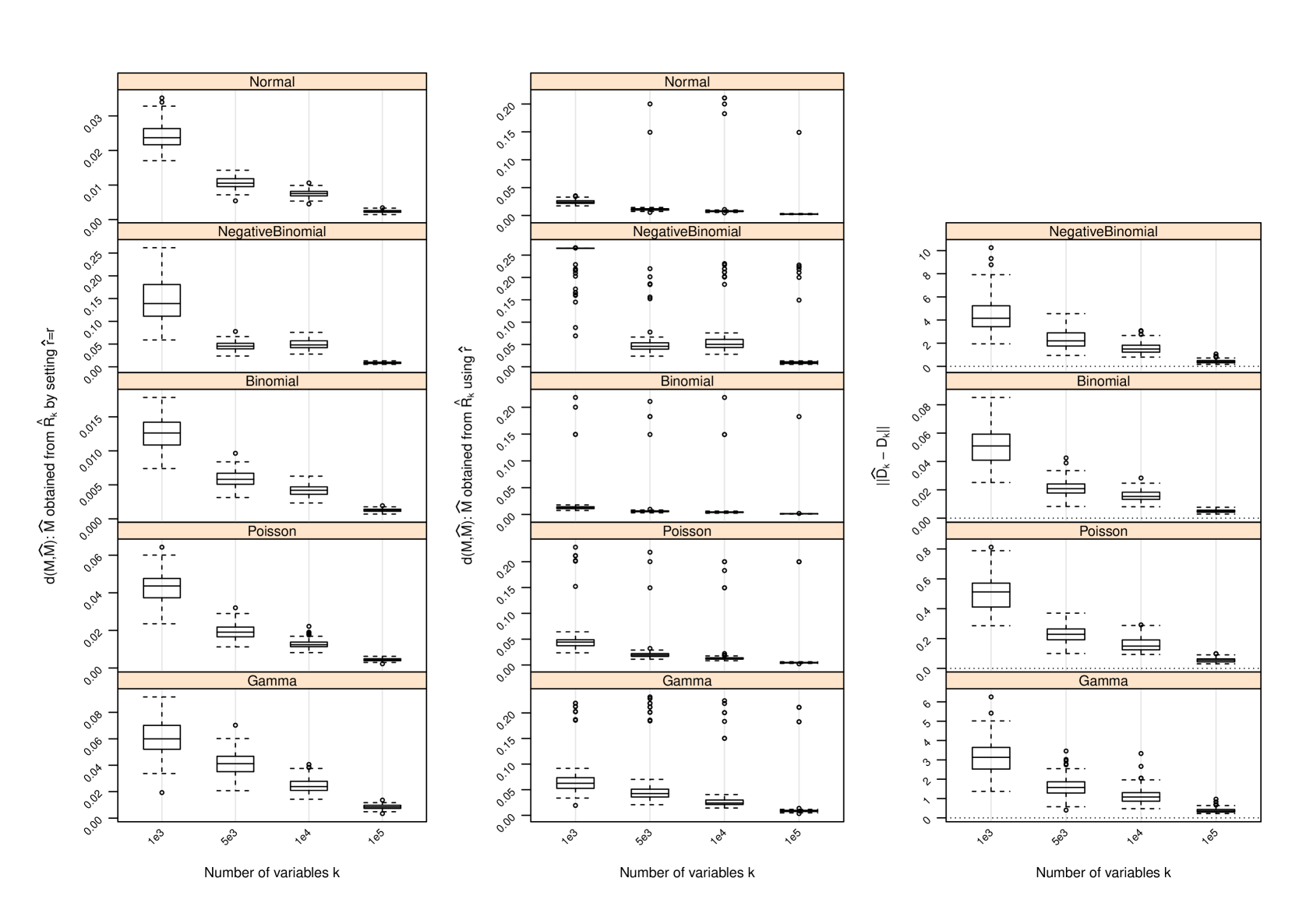
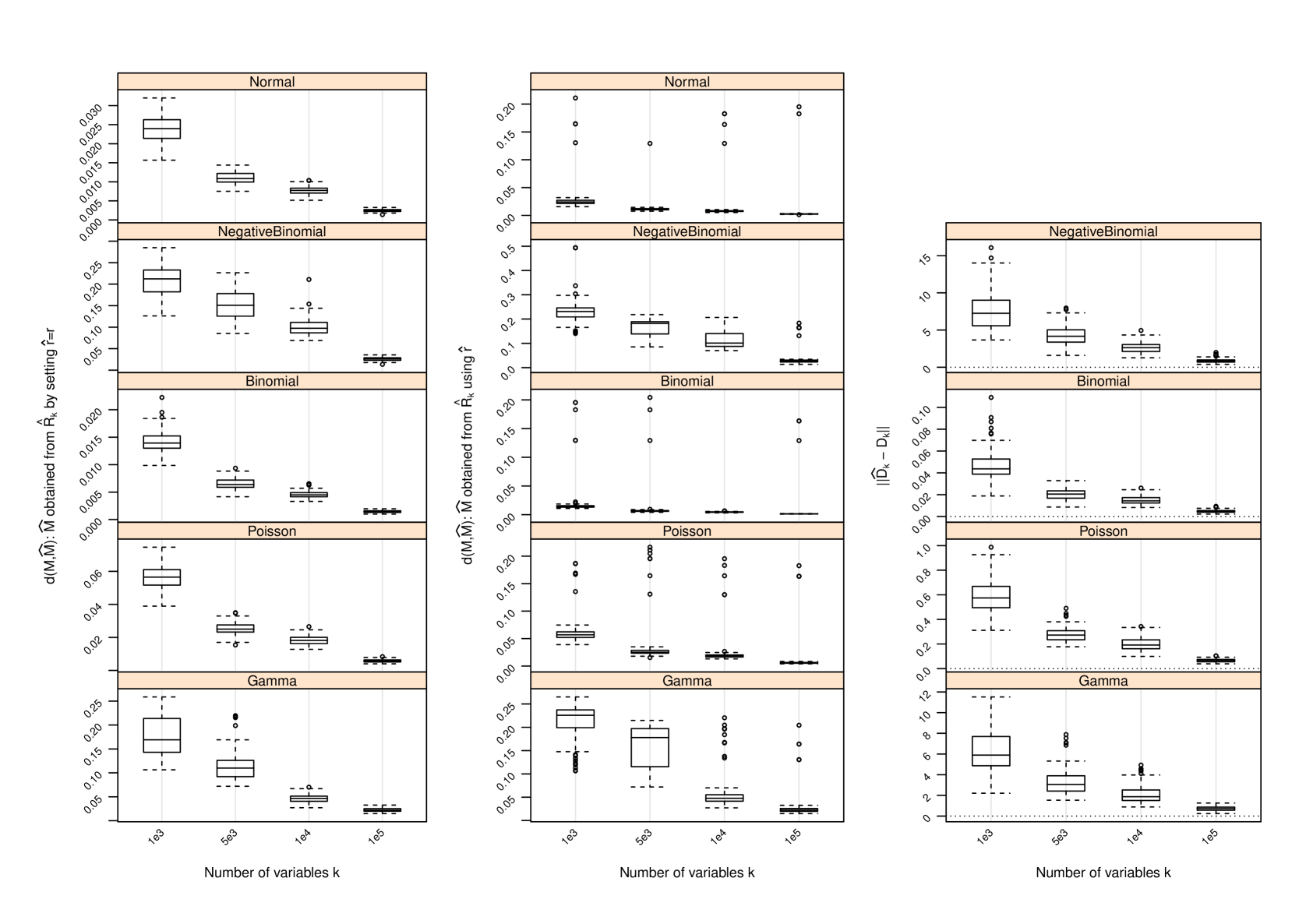
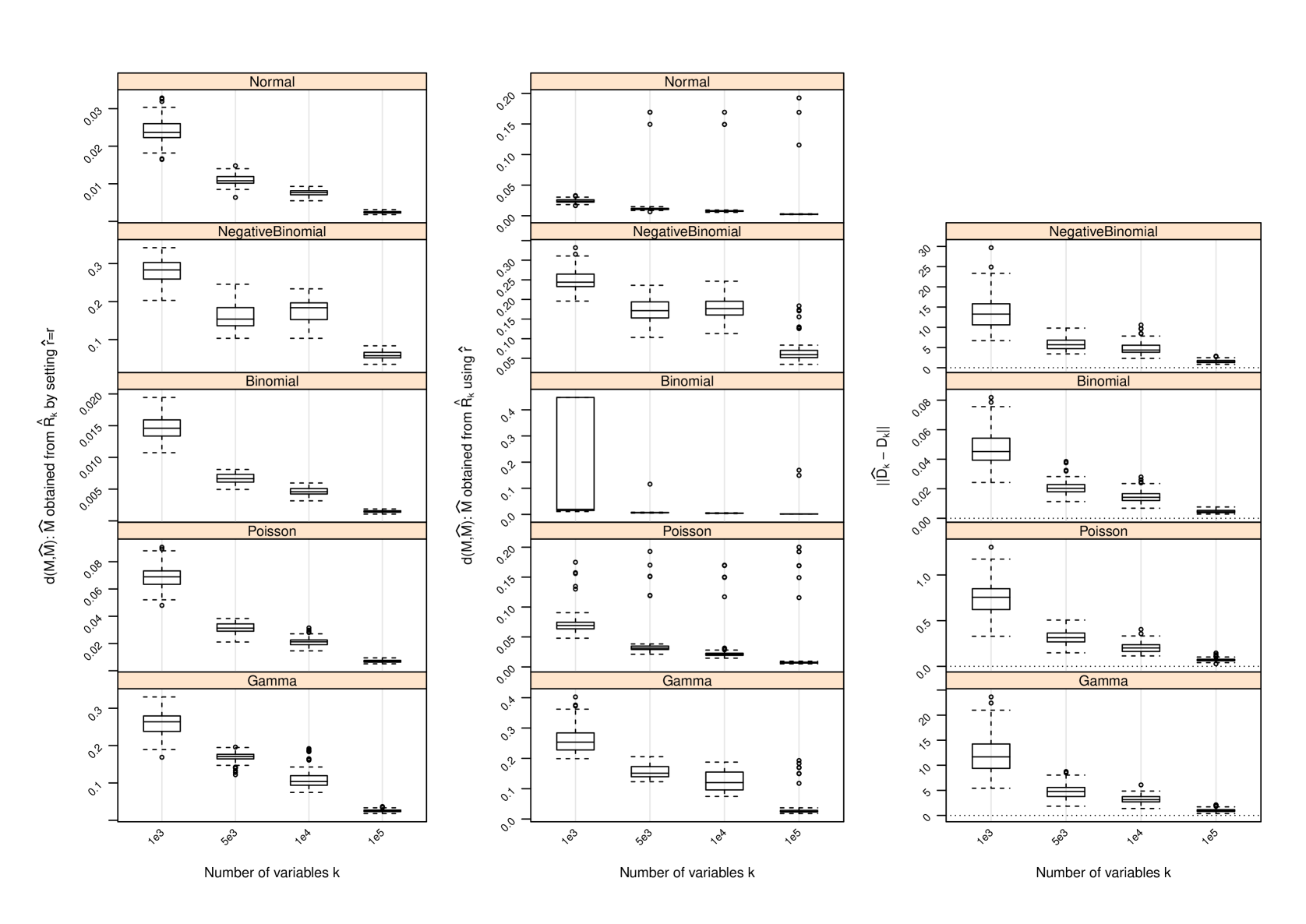
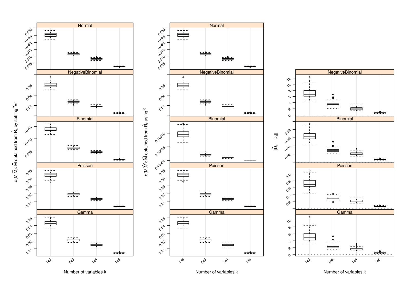
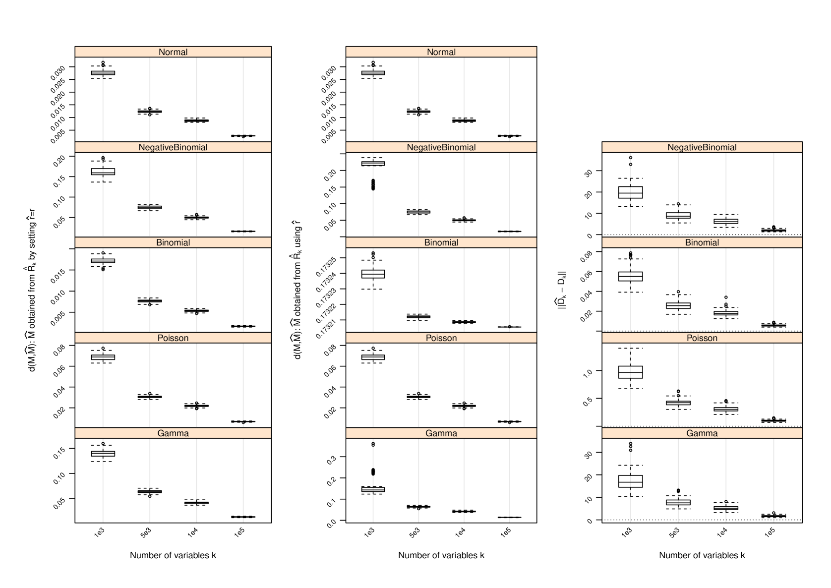
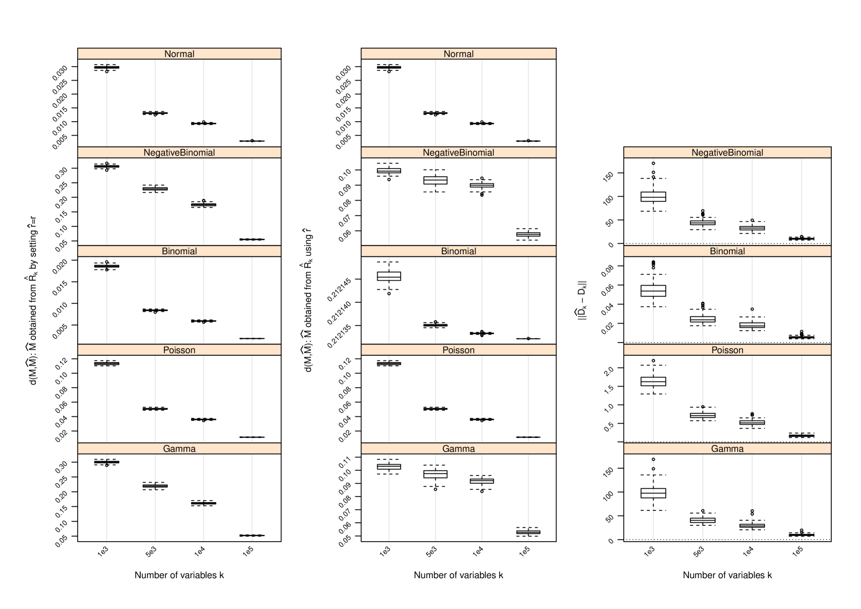
D Performance of Estimator of
The following figures show the performance of the nonparametric estimator of for several scenarios beyond that shown in Figure 1. The results are given over a range of and values as indicated in the figure captions. Column 1: Boxplots of the difference between the row spaces spanned by and as measured by when the true dimension of is utilized to form (i.e., setting ). Column 2: Boxplots of when using the proposed estimator of the row space dimension in forming . Column 3: An assessment of the estimate of , where the latter term is the average of the column-wise variances of . The difference is measured by .