Constant sectional curvature surfaces with a semi-symmetric non-metric connection
Abstract.
Consider the Euclidean space endowed with a canonical semi-symmetric non-metric connection determined by a vector field . We study surfaces when the sectional curvature with respect to this connection is constant. In case that the surface is cylindrical, we obtain full classification when the rulings are orthogonal or parallel to . If the surface is rotational, we prove that the rotation axis is parallel to and we classify all conical rotational surfaces with constant sectional curvature. Finally, for the particular case of the sectional curvature, the existence of rotational surfaces orthogonally intersecting the rotation axis is also obtained.
Key words and phrases:
rotational surface; sectional curvature; semi-symmetric connection; non-metric connection1991 Mathematics Subject Classification:
53B40, 53C42, 53B201. Introduction
Friedmann and Schouten introduced in 1924 the notion of a semi-symmetric connection in a Riemannian manifold [4]. An affine connection in a Riemannian manifold is said to be semi-symmetric connection if there is a non-zero vector field such that its torsion satisfies the identity
| (1) |
If in addition , the connection is called a semi-symmetric metric connection [6]. Yano studied semi-symmetric metric connections with zero curvature and when the covariant derivative of the torsion tensor vanishes [14]. Submanifolds of Riemannian manifolds with semi-symmetric metric connections have been also investigated: without aiming a complete list, we refer to the readers to [7, 8, 9, 10, 12, 13].
If , the connection is called semi-symmetric non-metric connection (snm-connection to abbreviate) [1, 2]. In this case, there is a relation between and the Levi-Civita connection of , namely,
| (2) |
Such as it occurs for semi-symmetric metric connections, it is natural to study submanifolds of Riemannian manifolds endowed with a snm-connection . Let be a submanifold of . Denote by (resp. ) the induced connection on by (resp. ). The Gauss formulas are given by
for all , where is a -tensor field on and is the second fundamental form of . It is known that [2]. Hence that problems of extrinsic nature are the same one that for the Levi-Civita connection.
We consider intrinsic geometry of submanifolds. One of the main concepts in intrinsic Riemannian geometry is that of sectional curvature. It is natural to carry this concept for snm-connections. However, the sectional curvature of with respect to cannot be defined by the usual way as the Levi-Civita connection . This is because if is the curvature tensor of , the quantity , where is an orthonormal basis of , depends on the basis : see Sect. 2 for details. In contrast, the third author of this paper, jointly with I. Mihai, proved that is independent on the basis [11]. Then they introduced the following notion of sectional curvature for snm-connections.
Definition 1.1.
Let be a Riemannian manifold endowed with a snm-connection . If is a plane in with an orthonormal basis , then the sectional curvature of with respect to is defined by
| (3) |
Once we have the notion of sectional curvature, it is natural to ask for those submanifolds with constant sectional curvature. As for the Levi-Civita connection, this question is difficult to address in all its generality.
In this paper, we consider that the ambient space is the -dimensional Euclidean space endowed with the Euclidean metric . The amount of snm-connections of is given by the vector fields in the definition (1) of a semi-symmetric connection. One of the simplest choices of snm-connections of is that is a canonical vector field. To be precise, let be canonical coordinates of and let be the corresponding basis of . In fact, if the vector field is assumed to be canonical, namely then, after a change of coordinates of , is a unit constant vector field.
Definition 1.2.
A snm-connection on is said to be canonical if is a unit constant vector field.
From now on, unless otherwise specified, we denote by a unit constant vector field on .
Definitively, the problem that we study is the classification of surfaces with constant sectional curvature for a given canonical snm-connection of . A way to tackle this problem is to impose a certain geometric condition on the surface. A natural condition is that the surface is invariant by a one-parameter group of rigid motions. Denote by the sectional curvature with respect to the induced connection on the surface from . Assuming a certain invariance of the surface, it allows us to expect that the equation can be expressed as an ordinary differential equation, where, under mild conditions, the existence is assured. For example, we can assume that the surface is invariant by a group of translations or that the surface is invariant by a group of rotations. In the first case, the surface is called cylindrical and in the second one, rotational surface, or surface of revolution.
The organization of this paper is according to both types of surfaces. In Sect. 2 we prove an useful formula for computing the sectional curvature of a surface in terms of that of and the Gaussian and mean curvatures of the surface. We will show some explicit examples of computations of sectional curvatures.
Section 3 is devoted to cylindrical surfaces. A cylindrical surface can be parametrized by , , , where is a unitary vector and is a curve contained in a plane orthogonal to . The surface is invariant by the group of translations generated by . After computing the sectional curvature in Thm. 3.1, in Cor. 3.2, we prove that any cylindrical surface whose rulings are parallel to has constant sectional curvature , being . Another interesting case of cylindrical surfaces is that the rulings are orthogonal to . We obtain a full classification of these cylindrical surfaces with constant depending on the sign of (Cor. 3.3). For the particular values and , in Cor. 3.4 we obtain explicit parametrizations of the surfaces.
Rotational surfaces are invariant by rotations about an axis of and such surfaces with constant will be studied in Sect. 4. It is worth to point out that there is not a priori relation between the axis and the vector field that defines the canonical snm-connection. However, we prove in Thm. 4.1 that and must be parallel. In Thm. 4.3, we classify all conical rotational surfaces with constant proving that these surfaces are planes or circular cylinders. As a last observation, when , in Thm. 4.5, the existence of rotational surfaces orthogonally intersecting the rotation axis is also obtained.
2. Preliminaries
Let be a Riemannian manifold of dimension and let be an affine connection on . The torsion and curvature of are respectively a -tensor field and a -tensor field defined by
for . Let be a snm-connection on determined by a vector field . Using (2), there is also a relation between and the Riemannian curvature tensor of ([1, 11]). Indeed, for orthonormal vectors , , we have
Although the first term at the right hand-side is the sectional curvature of the plane section , the term at the left hand-side depends on the choice of the basis of . Therefore, the value does not stand for a sectional curvature. The quantity (3) was proposed in [11] as the definition of sectional curvature of with respect to because it is independent on the basis in . In case that is an arbitrary basis of , it is immediate to see
| (4) |
From now on, suppose that is the Euclidean space . We compute the sectional curvature of a plane of .
Proposition 2.1.
Let be a canonical snm-connection on . If is a plane of , then its sectional curvature is
where is an orthonormal basis of . As a consequence, is constant with . Furthermore, (resp. ) if and only if is perpendicular to (resp. is parallel to ).
Proof.
Using (2) we compute
and
Also it is easy to see . Hence the curvature tensor is determined by
This gives the formula for . The last statement is a consequence of this formula. ∎
Remark 2.2.
The notion of scalar curvature at a point with respect to a snm-connection can be introduced in a similar manner as for the Levi-Civita connection. Let be an orthonormal basis of , . The scalar curvature with respect to is defined by
If is canonical, then by Prop. 2.1 the scalar curvature is constant, namely , for every .
We conclude this section establishing a relation between the sectional curvatures and of a surface in in terms of the Gaussian and the mean curvatures of the surface. Let be an oriented surface immersed in and its unit normal vector field. Let also be a snm-connection on determined by an arbitrary vector field . We have the decomposition of in its tangential and normal components with respect to ,
If , then the Gauss equation with respect to is ([2]):
| (5) |
Proposition 2.3.
Let be an oriented surface in and denote by and the Gaussian curvature and the mean curvature of , respectively, with respect to the Levi-Civita connection. Then
| (6) |
Moreover, if then there is an orthogonal basis of such that
| (7) |
where and are the coefficients of the second fundamental form .
Proof.
Since the codimension of in is , it has trivially flat normal bundle. Let be an orthogonal basis of such that and , where are the coefficients of the second fundamental form of with respect to the Levi-Civita connection: see [3, Props. 3.1 and 3.2]. Therefore we have because . By the Gauss equation (5) we obtain (7). With respect to this basis, we have
Identity (6) is a consequence of (7) and formulas (4) for and . ∎
Remark 2.4.
Identity (6) is satisfied for any vector field . Notice also that is invariant by translations of . This is because and do no change, as well as because a plane is not affected by translations. However, rigid motions change the value of and, consequently of . This is because of the presence of the vector field in (2) for computing the successive covariant derivatives.
Simple consequences of the relation (6) appear in the following result.
Corollary 2.5.
-
(1)
For a plane, we have . In particular, and equality holds if and only if the plane is orthogonal to the vector field .
-
(2)
For a cylindrical surface whose rulings are parallel to , we have .
Proof.
It is immediate because for a plane we have , and for a cylindrical surface with rulings parallel to we have and . ∎
Thanks to this corollary we see that a plane and a cylindrical cylinder satisfy the equality . In general, a surface satisfies if and only if . In case that is a canonical vector field, we construct such a surface as follows.
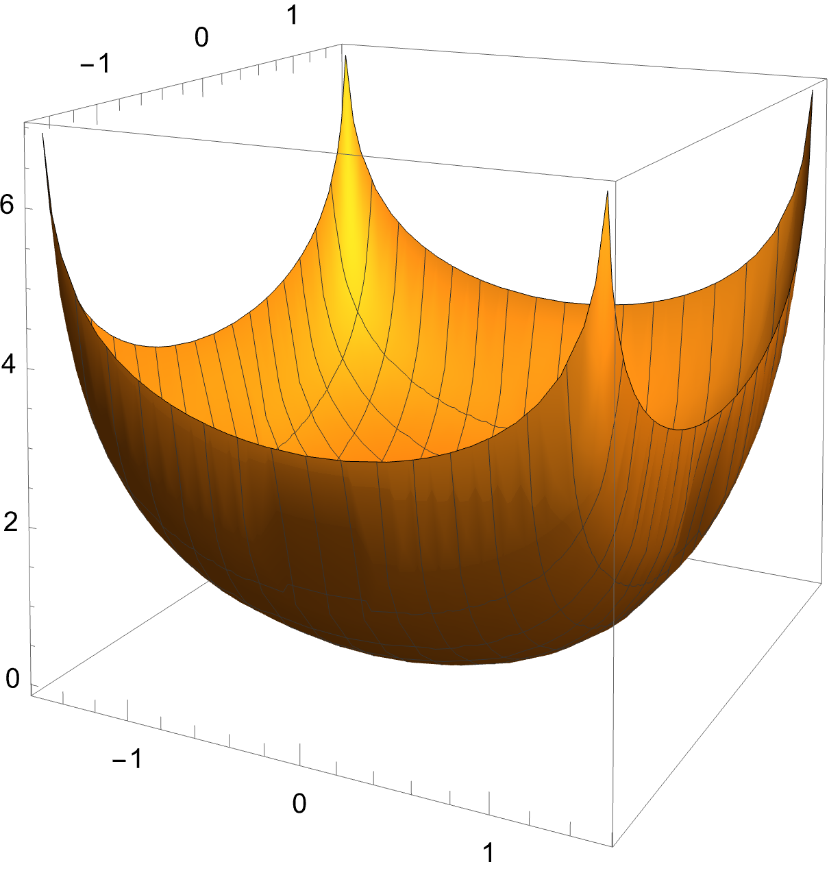
Example 2.6.
Let . To find a surface satisfying , we consider surfaces that are graphs of smooth functions , where . Then it is not difficult to find that the relation is written by
We find solutions of this equation by the technique of separation of variables. Assuming , for smooth functions and , , , the above equation becomes
| (8) |
for all , . Here a prime denotes the derivative with respect to each variable. A solution of Eq. (8) appears when and are linear functions, identically. Then is a plane parallel to the -plane. We discard this case by assuming on . Dividing Eq. (8) by , we obtain
Since the left hand-side depends only on the variable and the right hand-side on the variable , then we deduce the existence of the nonzero constant such that
Notice that if , then , which it is not possible. By solving these equations, we obtain, up to translations of and and suitable constants,
See Fig. 1 for the particular case .
3. Cylindrical surfaces
Let be a cylindrical surface in whose rulings are parallel to , where , . If is the generating curve of contained in a plane orthogonal to , then a parametrization of is
| (9) |
Without loss of generality, we suppose that is parametrized by arc-length. Let be the unit normal vector of and let be the Frenet curvature of with . Since is contained in a plane orthogonal to , consider the orientation on such that , where stands for the determinant of the matrix formed by three vectors , , of .
Theorem 3.1.
Let be a canonical snm-connection on . If is a cylindrical surface parametrized by (9), then its sectional curvature with respect to is
| (10) |
Proof.
The tangent plane of is spanned by an orthonormal basis , where and . We know that the Gaussian curvature is . The Gauss map and the mean curvature of are given by
We compute the covariant derivatives as follows
Because , we conclude that . We also compute
and thus
By (6) we find
The result follows because and . ∎
We distinguish two particular cases, when the rulings are parallel or orthogonal to the constant vector field .
Corollary 3.2.
Any cylindrical surface whose rulings are parallel to has constant sectional curvature with respect to a canonical snm-connection determined by .
Suppose that the rulings are orthogonal to . In the next result we are going to obtain explicit parametrizations of cylindrical surfaces with constant sectional curvature. Without loss of generality, we suppose that and . Then is contained in the -plane, say , for smooth functions . The case that is a plane is particular. Any plane of perpendicular to can be viewed as a cylindrical surface with rulings orthogonal to . By Prop. 2.1, we know that its curvature is constant with . We discard this case.
Corollary 3.3.
Let be the canonical snm-connection determined by and be a non-planar cylindrical surface whose rulings are orthogonal to . If the sectional curvature with respect to is constant, then the parametrization of the generating curve is
-
(1)
Case , then .
-
(2)
Case , then .
-
(3)
Case , then .
Proof.
Since is parametrized by arc-length, we know and . By the choice of orientation on given in Thm. 3.1, the normal vector is . Identity (10) is
The solution of this equation depends on the sign of . Up to an additive constant on the functions and as well as in the parameter , which it is only a translation of the surface (Rem. 2.4), we have
-
(1)
; then .
-
(2)
; then .
-
(3)
; then .
The result follows from the identity . ∎
In Fig. 2 we depict some graphics of the generating curves for different values of . Notice that the domain of is not in general because the root that appears in the integrals that define the -coordinate of . For example, if , then .
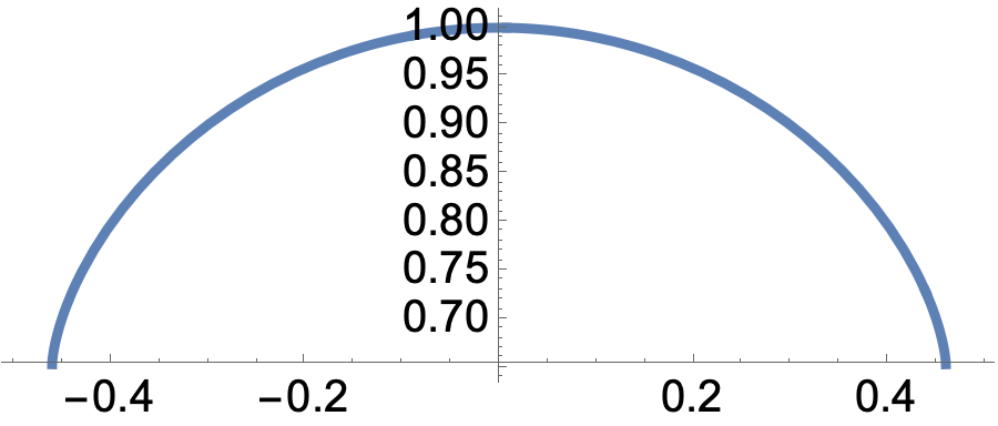
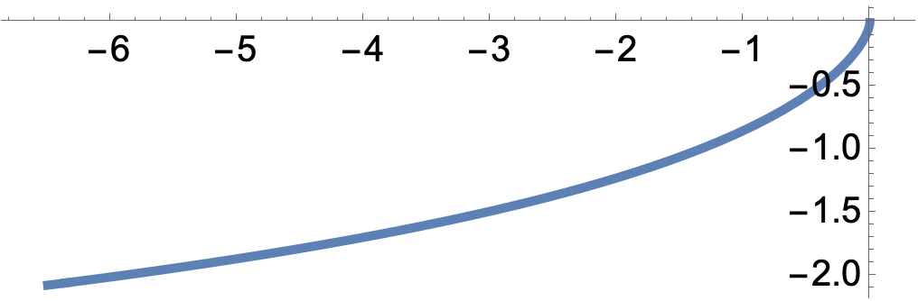
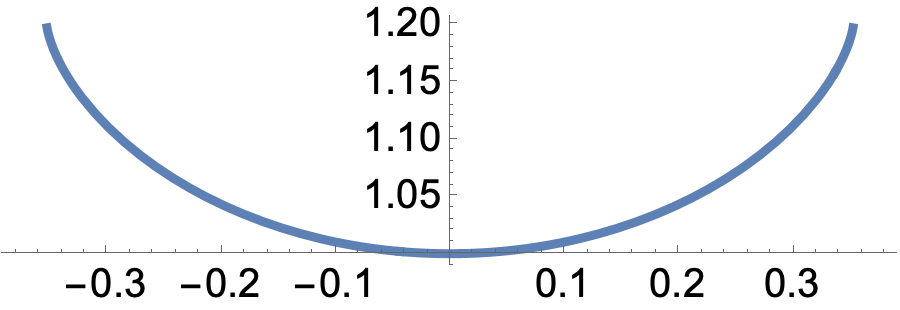
It is worth to consider the cases and . In such a case, the integrals of Cor. 3.3 can be explicitly solved.
Corollary 3.4.
Let be the canonical snm-connection determined by , a non-planar cylindrical surface whose rulings are orthogonal to , and the sectional curvature of with respect to .
-
(1)
If , then .
-
(2)
If , then .
For , the curve in (1) is called grim reaper. The usual parametrization of the grim reaper is in the -plane . This is deduced immediately by letting . The grim reaper is a remarkable curve in the theory of curve-shortening flow [5].
4. Rotational surfaces
In this section we study rotational surfaces with constant sectional curvature. A first problem is the relation between the axis of the surface and the vector field that defines the canonical snm-connection. As we said in the Introduction, there is no a priori a relation between both. However, we prove that they must be parallel.
Theorem 4.1.
Let be a canonical snm-connection on determined by the vector field and be a rotational surface in about an axis . If has constant sectional curvature , then either is any plane and or is parallel to .
Proof.
After a change of coordinates in , we can suppose that the axis of is the -axis. Let , for . Let also be the generating curve of which we can assume that it is contained in the -plane, namely,
We also assume that is parametrized by arc-length, that is, . Let be its Frenet curvature with respect to the induced Levi-Civita connection . A parametrization of is
For the computation of , we calculate all terms of (6). The tangent plane of is spanned by , where
The coefficients of the first fundamental form are , and . The unit normal vector of is
Then it is immediate
| (11) |
We now calculate . For this we employ the definition (3) taking into account that now the denominator is . We begin computing the covariant derivatives , . From (3), we have
Similarly, the covariant derivatives of second order are calculated. We obtain
Obviously, . The curvature is
This gives
Finally, using (6), we obtain
The above expression can be written as a polynomial equation of type
Since the functions , , are linearly independent, then all coefficients must vanish identically. The computation of these coefficients yields
From and , we have the following discussion of cases.
-
(1)
Case identically. Then is a constant function and this implies that is a horizontal plane. In particular, . Without loss of generality, we suppose . Since , equation is simply
This proves the result in this case.
-
(2)
Case that at some value . Then around and implies . Thus and this proves that is parallel to the -axis, which it is the rotation axis of .
∎
Once proved Thm. 4.1, we can suppose that the vector field is and is a rotational surface about the -axis. Following the proof of that theorem, all coefficients and , are trivially except which it is
Using the value of and given in (11), the above equation gives us the expression of of a rotational surface in terms of its generating curve, namely,
| (12) |
We study when the parenthesis of the right hand-side of (12) are identically.
Proposition 4.2.
If is constant in (12), then the functions and cannot vanish identically in .
Proof.
-
(1)
Case . Then neither nor can vanish identically. From (12), we have
Since , then
Combining both equations, we get , then is a constant function, which it is a contradiction.
-
(2)
Case . Since , then . Thus (12) is
On the other hand, it follows that
Combining both equations we obtain that is a constant function. From , we have constant too, which it is a contradiction by regularity of .
∎
In the following two results we study the case when the generating curve of has constant curvature , that is, is a straight-line and a circle. First, suppose that is a straight-line. This implies that is a conical rotational surface.
Theorem 4.3.
Let be a canonical snm-connection and be a rotational surface about the -axis. Assume that the sectional curvature of with respect to is constant. If the generating curve of is a straight-line, then either is a circular cylinder and , or is a horizontal plane and .
Proof.
We follow the notation of Thm. 4.1. Since is parametrized by arc-length, then there is a real number such that can be written as
Equation (12) is now
This is a polynomial equation on , so all coefficients must vanish. Therefore
-
(1)
Case . Then . In particular . This implies that is a circular cylinder of radius . The second equation gives .
-
(2)
Case . Then and the second equation gives . Thus and is a horizontal plane of equation . Here .
∎
Finally, we suppose that is a circle. This implies that is torus of revolution or a rotational ovaloid.
Theorem 4.4.
Let be a canonical snm-connection and be a rotational surface about the -axis. Assume that the sectional curvature of with respect to is constant. Then the generating curve of cannot be a circle.
Proof.
By contradiction, suppose that is a circle of radius . A parametrization of is
Substituting into (12), we obtain
This equation writes as
where and are real constants. Since all and must , a computation gives , obtaining a contradiction. ∎
The study of solutions of (12) is difficult to do in all its generality and Thms. 4.3 and 4.4 are the first results. An interesting value for is because this is the curvature of a circular cylinder (for any radius) and that of a plane parallel to . If , then Eq. (12) is
| (13) |
An interesting question is if this equation has a solution for curves starting orthogonally from the rotation axis. If is the time where intersects the -axis, then we need and . However, the left hand-side of (13) is not defined at . This implies that existence of such solutions is not assured. We prove that these solutions, indeed, exist.
Theorem 4.5.
There exist rotational surfaces with constant sectional curvature intersecting orthogonally the rotation axis.
Proof.
For our convenience, we work assuming that is locally a graph . Then
Then (13) becomes
or equivalently,
This equation also writes as
Thus there is an integration constant such that
If intersects orthogonally the -axis, then we have . This gives , obtaining a first integration of (12), namely,
Squaring both sides of this equation, we get
By standard theory of existence of ODE, this equation has a solution with initial value , proving the result. ∎
Acknowledgements
Rafael López is a member of the IMAG and of the Research Group “Problemas variacionales en geometría”, Junta de Andalucía (FQM 325). This research has been partially supported by MINECO/MICINN/FEDER grant no. PID2020-117868GB-I00, and by the “María de Maeztu” Excellence Unit IMAG, reference CEX2020-001105-M, funded by MCINN/AEI/10.13039/501100011033/ CEX2020-001105-M.
References
- [1] N. S. Agashe, A semi-symmetric non-metric connection on a Riemannian manifold. Indian J. Pure Appl. Math. 23 (1992), 399–409.
- [2] N. S. Agashe, M. R. Chafle, On submanifolds of a Riemannian manifold with a semi-symmetric non-metric connection. Tensor 55 (1994), 120–130.
- [3] B.-Y. Chen, Total mean curvature and submanifolds of finite type. Second edition. With a foreword by Leopold Verstraelen. Series in Pure Mathematics, 27. World Scientific Publishing Co. Pte. Ltd., Hackensack (2015).
- [4] A. Friedmann, J. A. Schouten, Über die Geometrie der halbsymmetrischen Übertragungen. Math. Z. 21 (1924), 211–223.
- [5] H. P. Halldorsson, Self-similar solutions to the curve shortening flow. Trans. Amer. Math. Soc. 364 (2012), 5285–5309.
- [6] H. Hayden, Subspaces of a space with torsion. Proc. London Math. Soc. 34 (1932), 27–50.
- [7] T. Imai, Hypersurfaces of a Riemannian manifold with semi-symmetric metric connection. Tensor (N. S.) 23 (1972), 300–306.
- [8] C. W. Lee, D. W. Yoon, J. W. Lee, Optimal inequalities for the Casorati curvatures of submanifolds of real space forms endowed with semi-symmetric metric connections. J. Inequal. Appl. 2014, 327 (2014).
- [9] A. Mihai, C. Özgür, Chen inequalities for submanifolds of real space forms with a semi-symmetric metric connection. Taiwan. J. Math. 4 (2010), 1465–1477.
- [10] A. Mihai and C. Özgür, Chen inequalities for submanifolds of complex space forms and Sasakian space forms endowed with semi-symmetric metric connections. Rocky Mountain J. Math. 41 (2011), 1653–1673.
- [11] A. Mihai, I. Mihai, A note on a well-defined sectional curvature of a semi-symmetric non-metric connection. Int. Electron. J. Geom. 17(1) (2024), 15-23.
- [12] Z. Nakao, Submanifolds of a Riemannian manifold with semisymmetric metric connections. Proc. Amer. Math. Soc. 54 (1976), 261–266.
- [13] Y. Wang, Minimal translation surfaces with respect to semi-symmetric connections in and . Bull. Korean Math. Soc. 58 (2021), 959–972.
- [14] K. Yano, On semi symmetric metric connection. Rev. Roum. Math. Pures Appl. 15 (1970), 1579–1591.