Constrained Attack-Resilient Estimation of Stochastic Cyber-Physical Systems

Wenbin Wan wenbinw2@illinois.edu Hunmin Kim kim_h@mercer.edu Naira Hovakimyan nhovakim@illinois.edu Petros Voulgaris pvoulgaris@unr.edu University of Illinois at Urbana-Champaign, USA Mercer University, USA University of Nevada, Reno, USA

Abstract

In this paper, a constrained attack-resilient estimation algorithm (CARE) is developed for stochastic cyber-physical systems. The proposed CARE can simultaneously estimate the compromised system states and attack signals. It has improved estimation accuracy and attack detection performance when physical constraints and operational limitations are available. In particular, CARE is designed for simultaneous input and state estimation that provides minimum-variance unbiased estimates, and these estimates are projected onto the constrained space restricted by inequality constraints subsequently. We prove that the estimation errors and their covariances from CARE are less than those from unconstrained algorithms and confirm that this property can further reduce the false negative rate in attack detection. We show that estimation errors of CARE are practically exponentially stable in mean square. Finally, an illustrative example of attacks on a vehicle is given to demonstrate the improved estimation accuracy and detection performance compared to an existing unconstrained algorithm.

keywords:

Detection, Kalman filtering, Recursive estimation, Stability, State estimation

^†^†journal:

\cortext

[cor1]Corresponding author.

1 Introduction

Cyber-Physical Systems (CPS) play a vital role in the metabolism of applications from large-scale industrial systems to critical infrastructures, such as smart grids, transportation networks, precision agriculture, and industrial control systems rajkumar2010cyber . Recent developments in CPS and their safety-critical applications have led to a renewed interest in CPS security. The interaction between information technology and the physical system has made control components of CPS vulnerable to malicious attacks cardenas2008research . Recent cases of CPS attacks have clearly illustrated their susceptibility and raised awareness of the security challenges in these systems. These include attacks on large-scale critical infrastructures, such as the German steel mill cyber attack lee2014german , and Maroochy Water breach slay2007lessons . Similarly, malicious attacks on avionics and automotive vehicles have been reported, such as the U.S. drone RQ-170 captured in Iran peterson2011iran , and disabling the brakes and stopping the engine on civilian cars koscher2010experimental ; checkoway2011comprehensive .

Related work

Traditionally, most works in the field of attack detection had only focused on monitoring the cyber-space misbehavior raiyn2014survey . With the emergence of CPS, it becomes vitally important to monitor physical misbehavior as well because the impact of the attack on physical systems also needs to be addressed cardenas2008secure . In the last decade, attention has been drawn from the perspective of the control theory that exploits some prior information on the system dynamics for detection and attack-resilient control. For instance, a unified modeling framework for CPS and attacks is proposed in pasqualetti2013attack . A typical control architecture for the networked system under both cyber and physical attacks is proposed in teixeira2012attack ; then attack scenarios, such as Denial-of-Service (DoS) and false-data injection (FDI) are analyzed using this control architecture in teixeira2015secure .

In recent years, model-based detection has been tremendously studied. Attack detection has been formulated as an $\ell_{0}$ / $\ell_{\infty}$ optimization problem, which is NP-hard pajic2014robustness . A convex relaxation has been studied in fawzi2014secure . Furthermore, the worst-case estimation error has been analyzed in pajic2017attack . Multirate sampled data controllers have been studied to guarantee detectability in NAGHNAEIAN201912 and to detect zero-dynamic attacks in 8796181 . A residual-based detector has been designed for power systems against false-data injection attacks, and the impact of attacks has been analyzed in liu2011false .

In addition, some papers have studied active detection, such as mo2009secure ; mo2014detecting , where the control input is watermarked with a pre-designed scheme that sacrifices optimality. The aforementioned methods have the problem that the state estimate is not resilient concerning the attack signal, and incorrect state estimates make it more challenging for defenders to react to malicious attacks consequently.

Attack-resilient estimation and detection problems have been studied to address the above challenge in yong2015resilients ; forti2016bayesian ; kim2020simultaneous , where attack detection has been formulated as a simultaneous input and state estimation problem, and the minimum-variance unbiased estimation technique has been applied. More specifically, the approach has been applied to linear stochastic systems in yong2015resilients , stochastic random set methods in forti2016bayesian , and nonlinear systems in kim2020simultaneous . These detection algorithms rely on statistical thresholds, such as the $\chi^{2}$ test, which is widely used in attack detection mo2014detecting ; teixeira2010cyber . Since the detection accuracy improves when the covariance decreases, a smaller covariance is desired.

On top of the minimum-variance estimation approach, the covariance can be further reduced when we incorporate the information of the input and state in terms of constraints. There have been several investigations on Kalman filtering with state constraints simon2002kalman ; ko2007state ; simon2010kalman ; kong2021kalman . The state constraints are induced by unmodeled dynamics and operational processes. Some of these examples include vision-aided inertial navigation mourikis2007multi , target tracking wang2002filtering and power systems yong2015simultaneous . Constraints on inputs are also considered, such as avoiding reachable dangerous states under the assumption that the attack input is constrained kafash2018constraining and designing a resilient controller based on the partial knowledge of the attacker in terms of inequality constraints djouadi2015finite . The methods in kafash2018constraining ; djouadi2015finite can efficiently be used to maneuver a class of attacks when input inequality constraints are available but cannot resiliently address the estimation problem due to the false-data injection. This problem remains to be solved with a stability guarantee in the presence of inequality constraints. In the current paper, we aim to solve the resilient estimation problem and investigate the stability and performance of the algorithm design that integrates with information aggregation. To the best of our knowledge, this is the first investigation that considers both state and input inequality constraints for attack-resilient estimation with guaranteed stability.

Contributions

Our main contributions of this work can be summarized as follows. i) We propose a constrained attack-resilient estimation algorithm (CARE) that can estimate the compromised system states and the attack signals simultaneously. CARE first provides minimum-variance unbiased estimates, and then they are projected onto the constrained space induced by information aggregation. ii) The proposed CARE has better estimation performance. We show that the projection strictly reduces the estimation errors and covariances. iii) We are the first to investigate the stability of the estimation algorithm with inequality constraints and prove that the estimation errors are practically exponentially stable in mean square. iv) The proposed CARE has better attack detection performance. We provide rigorous analysis that the false negative rate is reduced by using the proposed algorithm. v) The proposed algorithm is compared with the state-of-the-art method to show the improved estimation and attack detection performance.

Paper organization

The rest of the paper is organized as follows. Section 2 introduces notations, $\chi^{2}$ test for detection, and problem formulation. The high-level idea of the proposed algorithm is presented in Section 3.1. Section 3.2 gives a detailed algorithm derivation. Section 4 demonstrates the performance improvement and investigates the stability analysis of the proposed algorithm. Section 5 presents an illustrative example of vehicle attacks. Finally, Section 6 draws the conclusion.

2 Preliminaries

Notations

We use the subscript $k$ to denote the time index. For a real set ${\mathbb{R}}$ , ${\mathbb{R}}^{n}_{+}$ denotes the set of positive elements in the $n$ -dimensional Euclidean space and ${\mathbb{R}}^{n\times m}$ denotes the set of all $n\times m$ real matrices. For a matrix ${\bm{A}}$ , ${\bm{A}}^{\top}$ , ${\bm{A}}^{-1}$ , ${\bm{A}}^{\dagger}$ , $\operatorname*{\textit{diag}}({\bm{A}})$ , $\operatorname*{tr}({\bm{A}})$ and $\operatorname*{rank}({\bm{A}})$ denote the transpose, inverse, Moore-Penrose pseudoinverse, diagonal, trace and rank of ${\bm{A}}$ , respectively. For a symmetric matrix ${\bm{S}}$ , ${\bm{S}}>0$ ( ${\bm{S}}\geq 0$ ) indicates that ${\bm{S}}$ is positive (semi)definite. The matrix ${\bm{I}}$ denotes the identity matrix with an appropriate dimension. We use $\|\cdot\|$ to denote the standard Euclidean norm for vector or an induced matrix norm if it is not specified, ${\mathbb{E}}[\,\cdot\,]$ to denote the expectation operator, and $\times$ to denote matrix multiplication when the multiplied terms are in different lines. For a vector ${\bm{a}}$ , ${\bm{a}}(i)$ denotes the $i^{th}$ element in the vector ${\bm{a}}$ . Finally, vectors ${\bm{a}}$ , $\hat{{\bm{a}}}$ , $\tilde{{\bm{a}}}\triangleq{\bm{a}}-\hat{{\bm{a}}}$ denote the ground truth, estimate and estimation error of ${\bm{a}}$ , respectively.

$\chi^{2}$ Test for Detection

Given a sample of Gaussian random variable $\hat{\bm{\sigma}}_{k}$ with unknown mean $\bm{\sigma}_{k}$ and known covariance $\bm{\Sigma}_{k}$ , the $\chi^{2}$ test provides statistical evidence of whether $\bm{\sigma}_{k}=0$ or not. In particular, the sample $\hat{\bm{\sigma}}_{k}$ is being normalized by $\hat{\bm{\sigma}}_{k}^{\top}\bm{\Sigma}_{k}^{-1}\hat{\bm{\sigma}}_{k}$ , and we compare the normalized value with $\chi_{df}^{2}(\alpha)$ , where $\chi_{df}^{2}(\alpha)$ is the $\chi^{2}$ value with degree of freedom $df$ and statistical significance level $\alpha$ . We reject the null hypothesis $H_{0}$ : $\bm{\sigma}_{k}=0$ , if $\hat{\bm{\sigma}}_{k}^{\top}\bm{\Sigma}_{k}^{-1}\hat{\bm{\sigma}}_{k}>\chi^{2}_{df}(\alpha)$ , and accept alternative hypothesis $H_{1}$ : $\bm{\sigma}_{k}\neq 0$ , i.e., there is significant statistical evidence that $\bm{\sigma}_{k}$ is non-zero. Otherwise, we accept $H_{0}$ , i.e., there is no significant evidence that $\bm{\sigma}_{k}$ is non-zero.

False negative rate

Given a set of vectors $\{\bm{\sigma}_{k}\}$ , the false negative rate of the $\chi^{2}$ test is defined as the ratio of the number of false negative test results $N_{neg}$ and the number of non-zero vectors in the given set $N_{\bm{\sigma}_{k}\neq 0}$

\displaystyle F_{neg}(\{\hat{\bm{\sigma}}_{k}\},\{\bm{\Sigma}_{k}\})

\displaystyle\triangleq\frac{N_{neg}}{N_{\bm{\sigma}_{k}\neq 0}}=\frac{\sum_{k}(\bm{1}_{k})}{N_{\bm{\sigma}_{k}\neq 0}},

(1)

where

\displaystyle\bm{1}_{k}\triangleq\begin{cases}1,&\textit{if }\hat{\bm{\sigma}}_{k}^{\top}\bm{\Sigma}_{k}^{-1}\hat{\bm{\sigma}}_{k}\leq\chi^{2}_{df}(\alpha)\textit{ and }\bm{\sigma}_{k}\neq 0\\ 0,&\textit{otherwise}\end{cases}.

(2)

Problem Formulation

Consider the following linear time-varying (LTV) discrete-time stochastic system¹¹1 The current paper considers a general formulation for the attack input matrix ${\bm{G}}_{k}$ . If ${\bm{d}}_{k}$ is injected into the control input, then ${\bm{G}}_{k}={\bm{B}}_{k}$ . If ${\bm{d}}_{k}$ is directly injected into the system, then ${\bm{G}}_{k}={\bm{I}}$ .


$\displaystyle{\bm{x}}_{k+1}$	$\displaystyle={\bm{A}}_{k}{\bm{x}}_{k}+{\bm{B}}_{k}{\bm{u}}_{k}+{\bm{G}}_{k}{\bm{d}}_{k}+{\bm{w}}_{k}$	(3a)
$\displaystyle{\bm{y}}_{k}$	$\displaystyle={\bm{C}}_{k}{\bm{x}}_{k}+{\bm{v}}_{k},$	(3b)

where ${\bm{x}}_{k}\in\mathbb{R}^{m}$ , ${\bm{u}}_{k}\in\mathbb{R}^{n}$ and ${\bm{y}}_{k}\in\mathbb{R}^{n_{y}}$ are the state, the control input and the sensor measurement, respectively. The attack signal is modeled as a simultaneous input ${\bm{d}}_{k}\in\mathbb{R}^{n_{d}}$ , which is unknown to the defender. System matrices ${\bm{A}}_{k}$ , ${\bm{B}}_{k}$ , ${\bm{C}}_{k}$ and ${\bm{G}}_{k}$ are known and bounded with appropriate dimensions. We assume that $\operatorname*{rank}({\bm{C}}_{k}{\bm{G}}_{k-1})=n_{d}$ , $0\leq n_{d}\leq n_{y}$ . This is typical assumption as in yong2016unified ; kim2017attack . The interpretation of this assumption is that the impact of the attack ${\bm{d}}_{k-1}$ on the system dynamics can be observed by ${\bm{y}}_{k}$ . The process noise ${\bm{w}}_{k}$ and the measurement noise ${\bm{v}}_{k}$ are assumed to be i.i.d. Gaussian random variables with zero means and covariances ${\bm{Q}}_{k}\triangleq\mathbb{E}[{\bm{w}}_{k}{\bm{w}}_{k}^{\top}]\geq 0$ and ${\bm{R}}_{k}\triangleq\mathbb{E}[{\bm{v}}_{k}{\bm{v}}_{k}^{\top}]>0$ . Moreover, the measurement noise ${\bm{v}}_{k}$ , the process noise ${\bm{w}}_{k}$ , and the initial state ${\bm{x}}_{0}$ are uncorrelated with each other.

The adopted attack model in (3) is known as the FDI attack that is a very general type of attack, and includes physical attacks, Trojans, replay attacks, overflow bugs, packet injection, etc guo2018roboads . Because of this generality, this attack model has been widely used in CPS security literature (e.g., pasqualetti2013attack ; teixeira2015secure ; yong2015resilients ).

In the cyber-space, digital attack signals could be unconstrained, but their impact on the physical world is restricted by physical and operational constraints (i.e., ${\bm{x}}_{k}$ and ${\bm{d}}_{k}$ are constrained). For example, a vehicle has a limit on acceleration, velocity, steering angle, and change of steering angle. Any physical constraints and ability limitations on attack signals and states are presented by the inequality constraints

\displaystyle\mathcal{A}_{k}{\bm{d}}_{k}\leq{\bm{b}}_{k},\ \mathcal{B}_{k}{\bm{x}}_{k}\leq{\bm{c}}_{k},

(4)

where matrices $\mathcal{A}_{k}$ , $\mathcal{B}_{k}$ , and vectors ${\bm{b}}_{k}$ , ${\bm{c}}_{k}$ are known and bounded with appropriate dimensions. Throughout this paper, we assume that the feasible sets of the constraints in (4) are non-empty.

Remark 1

Gaussian noise in (3) is one of the general ways to model physical systems so that the filtering algorithms use this model to track the level of uncertainties. Therefore, many pieces of work consider Gaussian noise even in the presence of bounded constraints teixeira2009state ; simon2002kalman ; simon2010kalman .

Problem statement

Given the stochastic system in (3), we aim to design an attack-resilient estimation algorithm that can simultaneously estimate the compromised system state ${\bm{x}}_{k}$ and the attack signal ${\bm{d}}_{k}$ . In addition, we seek to improve estimation accuracy and detection performance with a stability guarantee when incorporating the information of the input and state in terms of constraints in (4).

Refer to caption — Figure 1: Constrained Attack-Resilient Estimation (CARE).

3 Algorithm Design

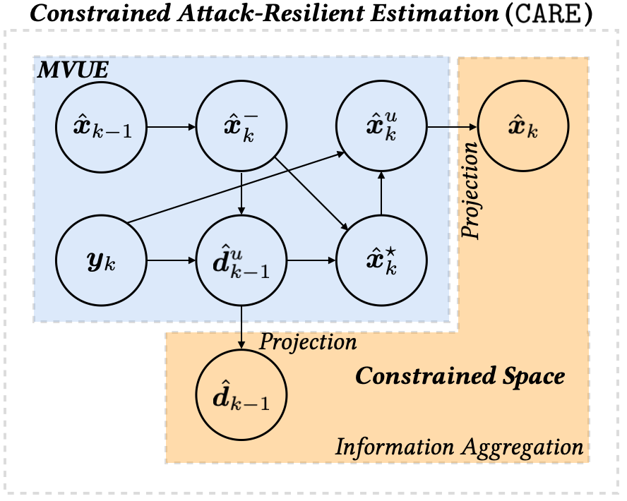
To address the problem statement described in Section 2, we propose a constrained attack-resilient estimation algorithm (CARE), as sketched in Fig. 1, which consists of a minimum-variance unbiased estimator (MVUE) and an information aggregation step via projection. In particular, the optimal estimation provides minimum-variance unbiased estimates, and these estimates are projected onto the constrained space eventually in the information aggregation step. We outline the essential steps of CARE in Section 3.1 and provide a detailed derivation of the algorithm in Section 3.2.

3.1 Algorithm Statement

The proposed CARE can be summarized as follows:

	$\displaystyle\textbf{prediction: }\hat{{\bm{x}}}_{k}^{-}={\bm{A}}_{k-1}\hat{{\bm{x}}}_{k-1}+{\bm{B}}_{k-1}{\bm{u}}_{k-1};$		(5)
	$\displaystyle\textbf{attack estimation: }\hat{{\bm{d}}}_{k-1}^{u}={\bm{M}}_{k}({\bm{y}}_{k}-{\bm{C}}_{k}\hat{{\bm{x}}}^{-}_{k});$		(6)
	$\displaystyle\textbf{time update: }\hat{{\bm{x}}}^{\star}_{k}=\hat{{\bm{x}}}^{-}_{k}+{\bm{G}}_{k-1}\hat{{\bm{d}}}^{u}_{k-1};$		(7)
	$\displaystyle\textbf{measurement update: }\hat{{\bm{x}}}^{u}_{k}=\hat{{\bm{x}}}^{\star}_{k}+{\bm{L}}_{k}({\bm{y}}_{k}-{\bm{C}}_{k}\hat{{\bm{x}}}^{\star}_{k});$		(8)
	projection update:

$\displaystyle\hat{{\bm{d}}}_{k-1}=$	$\displaystyle\operatorname*{arg\,min}_{\bm{d}}({\bm{d}}-\hat{{\bm{d}}}_{k-1}^{u})^{\top}({\bm{P}}_{k-1}^{d,u})^{-1}({\bm{d}}-\hat{{\bm{d}}}_{k-1}^{u})$
	$\displaystyle{\rm subject\ to\ }\mathcal{A}_{k-1}{\bm{d}}\leq{\bm{b}}_{k-1};$	(9)
$\displaystyle\hat{{\bm{x}}}_{k}=$	$\displaystyle\operatorname*{arg\,min}_{\bm{x}}({\bm{x}}-\hat{{\bm{x}}}^{u}_{k})^{\top}({\bm{P}}_{k}^{x,u})^{-1}({\bm{x}}-\hat{{\bm{x}}}^{u}_{k})$
	$\displaystyle{\rm subject\ to\ }\mathcal{B}_{k}{\bm{x}}\leq{\bm{c}}_{k}.$	(10)

Given the previous state estimate $\hat{{\bm{x}}}_{k-1}$ and its error covariance ${\bm{P}}_{k-1}^{x}\triangleq\mathbb{E}[\tilde{{\bm{x}}}_{k-1}(\tilde{{\bm{x}}}_{k-1})^{\top}]$ , the current state can be predicted by $\hat{{\bm{x}}}_{k}^{-}$ in (5) under the assumption that the attack signal ${\bm{d}}_{k-1}$ is absent. The unconstrained attack estimate $\hat{{\bm{d}}}_{k-1}^{u}$ can be obtained by comparing the difference between the predicted output ${\bm{C}}_{k}\hat{{\bm{x}}}_{k}^{-}$ and the measured output ${\bm{y}}_{k}$ in (6), where ${\bm{M}}_{k}$ is the optimal filter gain that can be obtained by applying Gauss-Markov theorem, as shown in Proposition 3 later. The state prediction $\hat{{\bm{x}}}_{k}^{-}$ can be updated incorporating the unconstrained attack estimate $\hat{{\bm{d}}}_{k-1}^{u}$ in (7). The output ${\bm{y}}_{k}$ is used to correct the current state estimate in (8), where ${\bm{L}}_{k}$ is the filter gain that is obtained by minimizing the state error covariance ${\bm{P}}_{k}^{x,u}$ . In the information aggregation step (projection update), we apply the input constraint in (9) by projecting $\hat{{\bm{d}}}_{k-1}^{u}$ onto the constrained space and obtain the constrained attack estimate $\hat{{\bm{d}}}_{k-1}$ . Similarly, the state constraint in (10) is applied to obtain the constrained state estimate $\hat{{\bm{x}}}_{k}$ . The complete algorithm is presented in Algorithm 1.

Algorithm 1 Constrained Attack-Resilient Estimation:

[\hat{{\bm{d}}}_{k-1}

{\bm{P}}^{d}_{k-1}

\hat{{\bm{x}}}_{k}

{\bm{P}}^{x}_{k}]=

CARE

(\hat{{\bm{x}}}_{k-1},{\bm{P}}^{x}_{k-1})

\triangleright

Prediction

\hat{{\bm{x}}}_{k}^{-}={\bm{A}}_{k-1}\hat{{\bm{x}}}_{k-1}+{\bm{B}}_{k-1}{\bm{u}}_{k-1}

;

{\bm{P}}_{k}^{x,-}={\bm{A}}_{k-1}{\bm{P}}^{x}_{k-1}{\bm{A}}_{k-1}^{\top}+{\bm{Q}}_{k-1}

;

\triangleright

Attack estimation

\tilde{{\bm{R}}}_{k}=({\bm{C}}_{k}{\bm{P}}_{k}^{x,-}{\bm{C}}_{k}^{\top}+{\bm{R}}_{k})^{-1}

;

{\bm{M}}_{k}=({\bm{G}}_{k-1}^{\top}{\bm{C}}_{k}^{\top}\tilde{{\bm{R}}}_{k}{\bm{C}}_{k}{\bm{G}}_{k-1})^{-1}{\bm{G}}_{k-1}^{\top}{\bm{C}}_{k}^{\top}\tilde{{\bm{R}}}_{k}

;

\hat{{\bm{d}}}_{k-1}^{u}={\bm{M}}_{k}({\bm{y}}_{k}-{\bm{C}}_{k}\hat{{\bm{x}}}_{k}^{-})

;

{\bm{P}}^{d,u}_{k-1}=({\bm{G}}_{k-1}^{\top}{\bm{C}}_{k}^{\top}\tilde{{\bm{R}}}_{k}{\bm{C}}_{k}{\bm{G}}_{k-1})^{-1}

;

{\bm{P}}_{k-1}^{xd}=-{\bm{P}}^{x}_{k-1}{\bm{A}}_{k-1}^{\top}{\bm{C}}_{k}^{\top}{\bm{M}}_{k}^{\top}

;

10:

\triangleright

Time update

11:

\hat{{\bm{x}}}^{\star}_{k}=\hat{{\bm{x}}}_{k}^{-}+{\bm{G}}_{k-1}\hat{{\bm{d}}}_{k-1}^{u}

;

12:

{\bm{P}}^{x\star}_{k}={\bm{A}}_{k-1}{\bm{P}}_{k-1}^{x}{\bm{A}}_{k-1}^{\top}+{\bm{A}}_{k-1}{\bm{P}}_{k-1}^{xd}{\bm{G}}_{k-1}^{\top}

13:

+{\bm{G}}_{k-1}({\bm{P}}_{k-1}^{xd})^{\top}{\bm{A}}_{k-1}^{\top}+{\bm{G}}_{k-1}{\bm{P}}_{k-1}^{d,u}{\bm{G}}_{k-1}^{\top}

14:

-{\bm{G}}_{k-1}{\bm{M}}_{k}{\bm{C}}_{k}{\bm{Q}}_{k-1}-{\bm{Q}}_{k-1}{\bm{C}}_{k}^{\top}{\bm{M}}_{k}^{\top}{\bm{G}}_{k-1}^{\top}

15:

+{\bm{Q}}_{k-1}

;

16:

\tilde{{\bm{R}}}^{\star}_{k}={\bm{C}}_{k}{\bm{P}}^{x\star}_{k}{\bm{C}}_{k}^{\top}-{\bm{C}}_{k}{\bm{G}}_{k-1}{\bm{M}}_{k}{\bm{R}}_{k}-{\bm{R}}_{k}{\bm{M}}_{k}^{\top}{\bm{G}}_{k-1}^{\top}{\bm{C}}_{k}^{\top}

17:

+{\bm{R}}_{k}

;

18:

\triangleright

Measurement update

19:

{\bm{L}}_{k}=({\bm{P}}^{x\star}_{k}{\bm{C}}_{k}^{\top}-{\bm{G}}_{k-1}{\bm{M}}_{k}{\bm{R}}_{k})\tilde{{\bm{R}}}^{\star\dagger}_{k}

;

20:

\hat{{\bm{x}}}^{u}_{k}=\hat{{\bm{x}}}^{\star}_{k}+{\bm{L}}_{k}({\bm{y}}_{k}-{\bm{C}}_{k}\hat{{\bm{x}}}^{\star}_{k})

;

21:

{\bm{P}}^{x,u}_{k}=({\bm{I}}-{\bm{L}}_{k}{\bm{C}}_{k}){\bm{G}}_{k-1}{\bm{M}}_{k}{\bm{R}}_{k}{\bm{L}}_{k}^{\top}

22:

+{\bm{L}}_{k}{\bm{R}}_{k}{\bm{M}}_{k}^{\top}{\bm{G}}_{k-1}^{\top}({\bm{I}}-{\bm{L}}_{k}{\bm{C}}_{k})^{\top}

23:

+({\bm{I}}-{\bm{L}}_{k}{\bm{C}}_{k}){\bm{P}}^{x\star}_{k}({\bm{I}}-{\bm{L}}_{k}{\bm{C}}_{k})^{\top}+{\bm{L}}_{k}{\bm{R}}_{k}{\bm{L}}_{k}^{\top}

;

24:

\triangleright

Projection update

25:

\bm{\gamma}_{k-1}^{d}={\bm{P}}_{k-1}^{d,u}\bar{\mathcal{A}}_{k-1}^{\top}(\bar{\mathcal{A}}_{k-1}{\bm{P}}_{k-1}^{d,u}\bar{\mathcal{A}}_{k-1}^{\top})^{-1}

;

26:

\hat{{\bm{d}}}_{k-1}=\hat{{\bm{d}}}_{k-1}^{u}-\bm{\gamma}_{k-1}^{d}(\bar{\mathcal{A}}_{k-1}\hat{{\bm{d}}}_{k-1}^{u}-\bar{{\bm{b}}}_{k-1})

;

27:

{\bm{P}}^{d}_{k-1}=({\bm{I}}-\bm{\gamma}_{k-1}^{d}\bar{\mathcal{{\bm{A}}}}_{k-1}){\bm{P}}^{d,u}_{k-1}({\bm{I}}-\bm{\gamma}_{k-1}^{d}\bar{\mathcal{A}}_{k-1})^{\top}

;

28:

\bm{\gamma}_{k}^{x}={\bm{P}}_{k}^{x,u}\bar{\mathcal{B}}_{k}^{\top}(\bar{\mathcal{B}}_{k}{\bm{P}}_{k}^{x,u}\bar{\mathcal{B}}_{k}^{\top})^{-1}

;

29:

\hat{{\bm{x}}}_{k}=\hat{{\bm{x}}}^{u}_{k}-\bm{\gamma}_{k}^{x}(\bar{\mathcal{B}}_{k}\hat{{\bm{x}}}^{u}_{k}-\bar{{\bm{c}}}_{k})

;

30:

{\bm{P}}^{x}_{k}=({\bm{I}}-\bm{\gamma}_{k}^{x}\bar{\mathcal{B}}_{k}){\bm{P}}^{x,u}_{k}({\bm{I}}-\bm{\gamma}_{k}^{x}\bar{\mathcal{B}}_{k})^{\top}

;

3.2 Algorithm Derivation

Prediction

The current state can be predicted by (5) under the assumption that the attack signal ${\bm{d}}_{k-1}=0$ . The prediction error covariance is

\displaystyle{\bm{P}}_{k}^{x{},-}\triangleq\mathbb{E}[\tilde{{\bm{x}}}_{k}^{-}(\tilde{{\bm{x}}}_{k}^{-})^{\top}]={\bm{A}}_{k-1}{\bm{P}}^{x{}}_{k-1}{\bm{A}}_{k-1}^{\top}+{\bm{Q}}_{k-1}.

(11)

Attack estimation

The linear attack estimator in (6) utilizes the difference between the measured output ${\bm{y}}_{k}$ and the predicted output ${\bm{C}}_{k}\hat{{\bm{x}}}^{-}_{k}$ . Substituting (3) and (5) into (6), we have

	$\displaystyle\hat{{\bm{d}}}_{k-1}^{u}={\bm{M}}_{k}\big{(}$	$\displaystyle{\bm{C}}_{k}{\bm{A}}_{k-1}\tilde{{\bm{x}}}_{k-1}+{\bm{C}}_{k}{\bm{G}}_{k-1}{\bm{d}}_{k-1}$
		$\displaystyle+{\bm{C}}_{k}{\bm{w}}_{k-1}+{\bm{v}}_{k}\big{)},$

which is a linear function of the attack signal ${\bm{d}}_{k-1}$ . Under the assumption that there is no projection update, i.e., the state and attack estimates are unconstrained, we design the optimal gain matrix ${\bm{M}}_{k}$ such that the estimate becomes the best linear unbiased estimate (BLUE) by the following two propositions.

Proposition 2

Assume that there is no projection update and $\mathbb{E}[\tilde{{\bm{x}}}_{0}]=\mathbb{E}[\tilde{{\bm{x}}}^{\star}_{0}]=0$ . The state estimates $\hat{{\bm{x}}}_{k}$ and the unconstrained attack estimates $\hat{{\bm{d}}}^{u}_{k}$ are unbiased for all $k$ , i.e. $\mathbb{E}[\tilde{{\bm{x}}}_{k}]=\mathbb{E}[\tilde{{\bm{d}}}^{u}_{k-1}]=0,\ \forall k$ , if and only if ${\bm{M}}_{k}{\bm{C}}_{k}{\bm{G}}_{k-1}={\bm{I}}$ .

Proof: Sufficiency: Assuming that ${\bm{M}}_{k}{\bm{C}}_{k}{\bm{G}}_{k-1}={\bm{I}}$ , the statement can be proved by induction. First, we will show the statement holds when $k=0$ as a base case. By the definition, the errors of the time update and the measurement update in (7) and (8) are given by

	$\displaystyle\tilde{{\bm{x}}}^{\star}_{k}$	$\displaystyle\triangleq{\bm{x}}_{k}-\hat{{\bm{x}}}^{\star}_{k}={\bm{A}}_{k-1}\tilde{{\bm{x}}}_{k-1}+{\bm{G}}_{k-1}\tilde{{\bm{d}}}^{u}_{k-1}+{\bm{w}}_{k-1}$		(12)
	$\displaystyle\tilde{{\bm{x}}}^{u}_{k}$	$\displaystyle\triangleq{\bm{x}}_{k}-\hat{{\bm{x}}}^{u}_{k}=({\bm{I}}-{\bm{L}}_{k}{\bm{C}}_{k})\tilde{{\bm{x}}}^{\star}_{k}-{\bm{L}}_{k}{\bm{v}}_{k},$		(13)

and the error of the unconstrained attack estimate is


$\displaystyle\tilde{{\bm{d}}}^{u}_{k-1}$	$\displaystyle\triangleq{\bm{d}}_{k-1}-\hat{{\bm{d}}}^{u}_{k-1}={\bm{d}}_{k-1}-{\bm{M}}_{k}\big{(}{\bm{C}}_{k}{\bm{A}}_{k-1}\tilde{{\bm{x}}}_{k-1}$
	$\displaystyle+{\bm{C}}_{k}{\bm{G}}_{k-1}{\bm{d}}_{k-1}+{\bm{C}}_{k}{\bm{w}}_{k-1}+{\bm{v}}_{k}\big{)}$
	$\displaystyle=({\bm{I}}-{\bm{M}}_{k}{\bm{C}}_{k}{\bm{G}}_{k-1}){\bm{d}}_{k-1}$	(14a)
	$\displaystyle-{\bm{M}}_{k}\big{(}{\bm{C}}_{k}{\bm{A}}_{k-1}\tilde{{\bm{x}}}_{k-1}+{\bm{C}}_{k}{\bm{w}}_{k-1}+{\bm{v}}_{k}\big{)}.$	(14b)

Under the assumptions that $\mathbb{E}[\tilde{{\bm{x}}}_{0}]=\mathbb{E}[\tilde{{\bm{x}}}^{\star}_{0}]=0$ and the process noise and measurement noise are zero-mean Gaussian, i.e. $\mathbb{E}[{\bm{w}}_{k}]=\mathbb{E}[{\bm{v}}_{k}]=0,\ \forall k$ , the expectation of the term (14b) is zero at $k=1$ . Since ${\bm{d}}_{k-1}$ is deterministic for all $k$ , i.e., $\mathbb{E}[{{\bm{d}}_{k-1}}]\neq 0$ , we have $\mathbb{E}[\tilde{{\bm{d}}}^{u}_{0}]=0$ if ${\bm{I}}-{\bm{M}}_{1}{\bm{C}}_{1}{\bm{G}}_{0}=0$ , i.e., the expectation of the term (14a) is zero at $k=1$ .Then we have $\mathbb{E}[\tilde{{\bm{x}}}^{\star}_{1}]=\mathbb{E}[\tilde{{\bm{x}}}^{u}_{1}]=0$ by applying expectation operation on (12) and (13). In the inductive step, suppose $\mathbb{E}[\tilde{{\bm{x}}}^{u}_{k}]=\mathbb{E}[\tilde{{\bm{x}}}^{\star}_{k}]=0$ ; then $\mathbb{E}[\tilde{{\bm{d}}}^{u}_{k}]=0$ if ${\bm{M}}_{k+1}{\bm{C}}_{k+1}{\bm{G}}_{k}={\bm{I}}$ . Then, similarly, we have $\mathbb{E}[\tilde{{\bm{x}}}^{\star}_{k+1}]=\mathbb{E}[\tilde{{\bm{x}}}^{u}_{k+1}]=0$ by (12) and (13). Since there is no projection update, we have $\mathbb{E}[\tilde{{\bm{x}}}_{k}]=\mathbb{E}[\tilde{{\bm{x}}}^{u}_{k}]=0\ \forall k$ .

Necessity: Assuming that $\mathbb{E}[\tilde{{\bm{x}}}_{k}]=\mathbb{E}[\tilde{{\bm{d}}}_{k-1}]=0$ for all $k$ , or equivalently $\mathbb{E}[\tilde{{\bm{x}}}^{u}_{k}]=\mathbb{E}[\tilde{{\bm{d}}}^{u}_{k-1}]=0$ , the statement also can be proved by induction. In (14), if $\mathbb{E}[\tilde{{\bm{d}}}^{u}_{0}]=0$ for any ${\bm{d}}_{0}$ , we have ${\bm{M}}_{1}{\bm{C}}_{1}{\bm{G}}_{0}={\bm{I}}$ . Therefore, following a similar procedure, we can show that the necessity holds. $\blacksquare$

Proposition 3

Assume that there is no projection update and $\mathbb{E}[\tilde{{\bm{x}}}_{0}]=\mathbb{E}[\tilde{{\bm{x}}}^{\star}_{0}]=0$ . The unconstrained attack estimates $\hat{{\bm{d}}}^{u}_{k}$ are BLUE if

\displaystyle{\bm{M}}_{k}=\big{(}{\bm{G}}_{k-1}^{\top}{\bm{C}}_{k}^{\top}\tilde{{\bm{R}}}_{k}{\bm{C}}_{k}{\bm{G}}_{k-1}\big{)}^{-1}{\bm{G}}_{k-1}^{\top}{\bm{C}}_{k}^{\top}\tilde{{\bm{R}}}_{k},

(15)

where $\tilde{{\bm{R}}}_{k}\triangleq({\bm{C}}_{k}{\bm{P}}_{k}^{x{},-}{\bm{C}}_{k}^{\top}+{\bm{R}}_{k})^{-1}$ .

Proof: Substituting (3a) into (3b), we have

	$\displaystyle{\bm{y}}_{k}$	$\displaystyle={\bm{C}}_{k}{\bm{G}}_{k-1}{\bm{d}}_{k-1}$
		$\displaystyle+{\bm{C}}_{k}\big{(}{\bm{A}}_{k-1}{\bm{x}}_{k-1}+{\bm{B}}_{k-1}{\bm{u}}_{k-1}+{\bm{w}}_{k-1}\big{)}+{\bm{v}}_{k}.$		(16)

Subtraction of ${\bm{C}}_{k}\hat{{\bm{x}}}_{k-1}$ on the both sides of (16) yields

	$\displaystyle{\bm{y}}_{k}-{\bm{C}}_{k}\hat{{\bm{x}}}_{k-1}$	$\displaystyle={\bm{C}}_{k}{\bm{G}}_{k-1}{\bm{d}}_{k-1}$
		$\displaystyle\underbrace{+{\bm{C}}_{k}\big{(}{\bm{A}}_{k-1}\tilde{{\bm{x}}}^{-}_{k-1}+{\bm{w}}_{k-1}\big{)}+{\bm{v}}_{k}}_{\textit{error term}}.$		(17)

Since the covariances of the process noise ${\bm{w}}_{k-1}$ and the measurement noise ${\bm{v}}_{k}$ are known, with (11), the covariance of the error term in (17) can be expressed as ${\bm{C}}_{k}{\bm{P}}_{k}^{x{},-}{\bm{C}}_{k}^{\top}+{\bm{R}}_{k}$ . Applying the Gauss-Markov theorem (see Appendix A), we can get the minimum-variance-unbiased linear estimator (BLUE) of ${\bm{d}}_{k-1}$ in (6) with ${\bm{M}}_{k}=\big{(}{\bm{G}}_{k-1}^{\top}{\bm{C}}_{k}^{\top}\tilde{{\bm{R}}}_{k}{\bm{C}}_{k}{\bm{G}}_{k-1}\big{)}^{-1}{\bm{G}}_{k-1}^{\top}{\bm{C}}_{k}^{\top}\tilde{{\bm{R}}}_{k}$ , where $\tilde{{\bm{R}}}_{k}\triangleq({\bm{C}}_{k}{\bm{P}}_{k}^{x{},-}{\bm{C}}_{k}^{\top}+{\bm{R}}_{k})^{-1}$ . $\blacksquare$

Remark 4

The rank condition $\operatorname*{rank}({\bm{C}}_{k}{\bm{G}}_{k-1})=n_{d}$ is the sufficient condition of ${\bm{M}}_{k}{\bm{C}}_{k}{\bm{G}}_{k-1}={\bm{I}}$ needed in Proposition 2 if ${\bm{M}}_{k}$ is found by (15) in Proposition 3.

The error covariance can be found by ${\bm{P}}_{k-1}^{d,u}={\bm{M}}_{k}\tilde{{\bm{R}}}_{k}^{-1}{\bm{M}}_{k}^{\top}=\big{(}{\bm{G}}_{k-1}^{\top}{\bm{C}}_{k}^{\top}\tilde{{\bm{R}}}_{k}{\bm{C}}_{k}{\bm{G}}_{k-1}\big{)}^{-1}.$ The cross error covariance of the state estimate and the attack estimate is ${\bm{P}}_{k-1}^{xd}=-{\bm{P}}^{x}_{k-1}{\bm{A}}_{k-1}^{\top}{\bm{C}}_{k}^{\top}{\bm{M}}_{k}^{\top}.$

Time update

Given the unconstrained attack estimate $\hat{{\bm{d}}}^{u}_{k-1}$ , the state prediction $\hat{{\bm{x}}}^{-}_{k}$ can be updated as in (7). We derive the error covariance of $\hat{{\bm{x}}}^{\star}_{k}$ as

	$\displaystyle{\bm{P}}_{k}^{x\star}$	$\displaystyle\triangleq\mathbb{E}\big{[}\tilde{{\bm{x}}}^{\star}_{k}(\tilde{{\bm{x}}}^{\star}_{k})^{\top}\big{]}$
		$\displaystyle={\bm{A}}_{k-1}{\bm{P}}_{k-1}^{x}{\bm{A}}_{k-1}^{\top}+{\bm{A}}_{k-1}{\bm{P}}_{k-1}^{xd}{\bm{G}}_{k-1}^{\top}$
		$\displaystyle+{\bm{G}}_{k-1}{\bm{P}}_{k-1}^{dx}{\bm{A}}_{k-1}^{\top}+{\bm{G}}_{k-1}{\bm{P}}_{k-1}^{d,u}{\bm{G}}_{k-1}^{\top}+{\bm{Q}}_{k-1}$
		$\displaystyle-{\bm{G}}_{k-1}{\bm{M}}_{k}{\bm{C}}_{k}{\bm{Q}}_{k-1}-{\bm{Q}}_{k-1}{\bm{C}}_{k}^{\top}{\bm{M}}_{k}^{\top}{\bm{G}}_{k-1}^{\top},$

where ${\bm{P}}_{k-1}^{dx}=({\bm{P}}_{k-1}^{xd})^{\top}$ .

Measurement update

In this step, the measurement ${\bm{y}}_{k}$ is used to update the propagated estimate $\hat{{\bm{x}}}^{\star}_{k}$ as shown in (8). The covariance of the state estimation error is

	$\displaystyle{\bm{P}}^{x,u}_{k}\triangleq$	$\displaystyle\mathbb{E}[(\tilde{{\bm{x}}}_{k}^{u})(\tilde{{\bm{x}}}_{k}^{u})^{\top}]$
	$\displaystyle=$	$\displaystyle({\bm{I}}-{\bm{L}}_{k}{\bm{C}}_{k}){\bm{G}}_{k-1}{\bm{M}}_{k}{\bm{R}}_{k}{\bm{L}}_{k}^{\top}+{\bm{L}}_{k}{\bm{R}}_{k}{\bm{L}}_{k}^{\top}$
		$\displaystyle+{\bm{L}}_{k}{\bm{R}}_{k}{\bm{M}}_{k}^{\top}{\bm{G}}_{k-1}^{\top}({\bm{I}}-{\bm{L}}_{k}{\bm{C}}_{k})^{\top}$
		$\displaystyle+({\bm{I}}-{\bm{L}}_{k}{\bm{C}}_{k}){\bm{P}}^{x\star}_{k}({\bm{I}}-{\bm{L}}_{k}{\bm{C}}_{k})^{\top}.$

The gain matrix ${\bm{L}}_{k}$ is obtained by minimizing the trace of ${\bm{P}}^{x,u}_{k}$ , i.e. $\min_{{\bm{L}}_{k}}\operatorname*{tr}({\bm{P}}^{x,u}_{k}).$ The solution is given by ${\bm{L}}_{k}=({\bm{P}}^{x\star}_{k}{\bm{C}}_{k}^{\top}-{\bm{G}}_{k-1}{\bm{M}}_{k}{\bm{R}}_{k})\tilde{{\bm{R}}}^{\star\dagger}_{k},$ where $\tilde{{\bm{R}}}^{\star}_{k}\triangleq{\bm{C}}_{k}{\bm{P}}^{x\star}_{k}{\bm{C}}_{k}^{\top}+{\bm{R}}_{k}-{\bm{C}}_{k}{\bm{G}}_{k-1}{\bm{M}}_{k}{\bm{R}}_{k}-{\bm{R}}_{k}{\bm{M}}_{k}^{\top}{\bm{G}}_{k-1}^{\top}{\bm{C}}_{k}^{\top}$ .

Projection update

We are now in the position to project the estimates onto the constrained space. Apply the first constraint in (4) to the unconstrained attack estimate $\hat{{\bm{d}}}_{k-1}^{u}$ , and the attack estimation problem can be formulated as the following constrained convex optimization problem

\displaystyle\begin{split}\hat{{\bm{d}}}_{k-1}&=\operatorname*{arg\,min}\limits_{\bm{d}}({\bm{d}}-\hat{{\bm{d}}}_{k-1}^{u})^{\top}{\bm{W}}^{d}_{k-1}({\bm{d}}-\hat{{\bm{d}}}_{k-1}^{u})\\ &\text{subject to}\ \mathcal{A}_{k-1}{\bm{d}}\leq{\bm{b}}_{k-1},\end{split}

(18)

where ${\bm{W}}^{d}_{k-1}$ can be any positive definite symmetric weighting matrix. In the current paper, we select ${\bm{W}}_{k-1}^{d}=({\bm{P}}_{k-1}^{d,u})^{-1}$ which results in the smallest error covariance as shown in simon2002kalman . From Karush-Kuhn-Tucker (KKT) conditions of optimality, we can find the corresponding active constraints. We denote $\bar{\mathcal{A}}_{k}$ and $\bar{{\bm{b}}}_{k}$ the rows of $\mathcal{A}_{k}$ and the elements of ${\bm{b}}_{k}$ corresponding to the active constraints of $\mathcal{A}_{k-1}{\bm{d}}\leq{\bm{b}}_{k-1}$ . Then (18) becomes

\displaystyle\begin{split}\hat{{\bm{d}}}_{k-1}&=\operatorname*{arg\,min}\limits_{\bm{d}}({\bm{d}}-\hat{{\bm{d}}}_{k-1}^{u})^{\top}({\bm{P}}_{k-1}^{d,u})^{-1}({\bm{d}}-\hat{{\bm{d}}}_{k-1}^{u})\\ &\text{subject to}\ \bar{\mathcal{A}}_{k-1}{\bm{d}}=\bar{{\bm{b}}}_{k-1}.\end{split}

(19)

The solution of (19) can be found by $\hat{{\bm{d}}}_{k-1}=\hat{{\bm{d}}}_{k-1}^{u}-\bm{\gamma}_{k-1}^{d}(\bar{\mathcal{A}}_{k-1}\hat{{\bm{d}}}_{k-1}^{u}-\bar{{\bm{b}}}_{k-1}),$ where

\displaystyle\bm{\gamma}_{k-1}^{d}

\displaystyle\triangleq{\bm{P}}_{k-1}^{d,u}\bar{\mathcal{A}}_{k-1}^{\top}(\bar{\mathcal{A}}_{k-1}{\bm{P}}_{k-1}^{d,u}\bar{\mathcal{A}}_{k-1}^{\top})^{-1}.

(20)

The attack estimation error is

	$\displaystyle\tilde{{\bm{d}}}_{k-1}$	$\displaystyle=({\bm{I}}-\bm{\gamma}_{k-1}^{d}\bar{\mathcal{A}}_{k-1})\tilde{{\bm{d}}}_{k-1}^{u}+\bm{\gamma}_{k-1}^{d}(\bar{\mathcal{A}}_{k-1}{\bm{d}}_{k-1}-\bar{{\bm{b}}}_{k-1})$
		$\displaystyle=\hat{{\bm{d}}}^{u}_{k-1}-\bm{\gamma}_{k-1}^{d}(\bar{\mathcal{A}}_{k-1}\hat{{\bm{d}}}^{u}_{k-1}-\bar{{\bm{b}}}_{k-1}).$		(21)

The error covariance can be found by

	$\displaystyle{\bm{P}}^{d}_{k-1}$	$\displaystyle\triangleq{\mathbb{E}}[\tilde{{\bm{d}}}_{k-1}\tilde{{\bm{d}}}_{k-1}^{\top}]$
		$\displaystyle=({\bm{I}}-\bm{\gamma}_{k-1}^{d}\bar{\mathcal{A}}_{k-1}){\bm{P}}^{d,u}_{k-1}({\bm{I}}-\bm{\gamma}_{k-1}^{d}\bar{\mathcal{A}}_{k-1})^{\top}$		(22)

under the assumption that $\bm{\gamma}_{k-1}^{d}(\bar{\mathcal{A}}_{k-1}{\bm{d}}_{k-1}-\bar{{\bm{b}}}_{k-1})=0$ holds. Notice that this assumption holds when the ground truth ${\bm{d}}_{k-1}$ satisfies the active constraint $\bar{\mathcal{A}}_{k-1}{\bm{d}}_{k-1}=\bar{{\bm{b}}}_{k-1}$ . From (20), it can be verified that $\bm{\gamma}_{k-1}^{d}\bar{\mathcal{A}}_{k-1}{\bm{P}}^{d,u}_{k-1}=\bm{\gamma}_{k-1}^{d}\bar{\mathcal{A}}_{k-1}{\bm{P}}^{d,u}_{k-1}(\bm{\gamma}_{k-1}^{d}\bar{\mathcal{A}}_{k-1})^{\top}$ . Therefore, from (22) we have

$\displaystyle{\bm{P}}^{d}_{k-1}=$	$\displaystyle{\bm{P}}^{d,u}_{k-1}-\bm{\gamma}_{k-1}^{d}\bar{\mathcal{A}}_{k-1}{\bm{P}}^{d,u}_{k-1}-{\bm{P}}^{d,u}_{k-1}(\bm{\gamma}_{k-1}^{d}\bar{\mathcal{A}}_{k-1})^{\top}$
	$\displaystyle+\bm{\gamma}_{k-1}^{d}\bar{\mathcal{A}}_{k-1}{\bm{P}}^{d,u}_{k-1}(\bm{\gamma}_{k-1}^{d}\bar{\mathcal{A}}_{k-1})^{\top}$
$\displaystyle=$	$\displaystyle({\bm{I}}-\bm{\gamma}_{k-1}^{d}\bar{\mathcal{A}}_{k-1}){\bm{P}}^{d,u}_{k-1}.$	(23)

Similarly, applying the second constraint in (4) to the unconstrained state estimate $\hat{{\bm{x}}}_{k}^{u}$ , we formalize the state estimation problem as follows:

\displaystyle\begin{split}\hat{{\bm{x}}}_{k}&=\operatorname*{arg\,min}_{{\bm{x}}}({\bm{x}}-\hat{{\bm{x}}}^{u}_{k})^{\top}{\bm{W}}^{x}_{k}({\bm{x}}-\hat{{\bm{x}}}^{u}_{k})\\ &\text{subject to}\ \mathcal{B}_{k}{\bm{x}}\leq{\bm{c}}_{k},\end{split}

(24)

where we select ${\bm{W}}^{x}_{k}=({\bm{P}}^{x,u}_{k})^{-1}$ for the smallest error covariance. We denote $\bar{\mathcal{B}}_{k}$ and $\bar{{\bm{c}}}_{k}$ the rows of $\mathcal{B}_{k}$ and the elements of ${\bm{c}}_{k}$ corresponding to the active constraints of $\mathcal{B}_{k}{\bm{x}}\leq{\bm{c}}_{k}$ . Using the active constraints, we reformulate (24) as follows:

\displaystyle\begin{split}\hat{{\bm{x}}}_{k}&=\operatorname*{arg\,min}\limits_{\bm{x}}({\bm{x}}-\hat{{\bm{x}}}^{u}_{k})^{\top}({\bm{P}}^{x,u}_{k})^{-1}({\bm{x}}-\hat{{\bm{x}}}^{u}_{k})\\ &\text{subject to}\ \bar{\mathcal{B}}_{k}{\bm{x}}=\bar{{\bm{c}}}_{k}.\end{split}

(25)

The solution of (25) is given by $\hat{{\bm{x}}}_{k}=\hat{{\bm{x}}}^{u}_{k}-\bm{\gamma}_{k}^{x}(\bar{\mathcal{B}}_{k}\hat{{\bm{x}}}^{u}_{k}-\bar{{\bm{c}}}_{k}),$ where

\displaystyle\bm{\gamma}_{k}^{x}

\displaystyle\triangleq{\bm{P}}^{x,u}_{k}\bar{\mathcal{B}}_{k}^{\top}(\bar{\mathcal{B}}_{k}{\bm{P}}^{x,u}_{k}\bar{\mathcal{B}}_{k}^{\top})^{-1}.

(26)

Under the assumption that $\bm{\gamma}_{k}^{x}(\bar{\mathcal{B}}_{k}\hat{{\bm{x}}}^{u}_{k}-\bar{{\bm{c}}}_{k})=0$ holds, the state estimation error covariance can be expressed as

\displaystyle{\bm{P}}^{x}_{k}

\displaystyle=\bar{\bm{\Gamma}}_{k}{\bm{P}}^{x,u}_{k}\bar{\bm{\Gamma}}_{k}^{\top},

(27)

where $\bar{\bm{\Gamma}}_{k}\triangleq{\bm{I}}-\bm{\gamma}_{k}^{x}\bar{\mathcal{B}}_{k}$ . Notice that this assumption holds when the ground truth ${\bm{x}}_{k}$ satisfies the active constraint $\bar{\mathcal{B}}_{k}{\bm{x}}_{k}=\bar{{\bm{c}}}_{k}$ .

4 Performance and Stability Analysis

In Section 4.1, we show that the projection induced by inequality constraints improves attack-resilient estimation accuracy and detection performance by decreasing estimation errors and the false negative rate in attack detection. Notice that the estimate $\hat{{\bm{d}}}_{k-1}$ and the ground truth ${\bm{d}}_{k-1}$ satisfy the active constraint $\bar{\mathcal{A}}_{k-1}\hat{{\bm{d}}}_{k-1}-\bar{{\bm{b}}}_{k-1}=0$ in (19) and the inequality constraint $\mathcal{A}_{k-1}{\bm{d}}_{k-1}\leq{\bm{b}}_{k-1}$ in (4), respectively. However, it is uncertain whether the ground truth satisfies the active constraints or not. In this case, from (21) we have

\displaystyle\mathbb{E}[\tilde{{\bm{d}}}_{k-1}]

\displaystyle=\bm{\gamma}_{k-1}^{d}(\bar{\mathcal{A}}_{k-1}{\bm{d}}_{k-1}-\bar{{\bm{b}}}_{k-1})\neq 0.

(28)

A similar statement holds for the state estimation error:

\displaystyle\mathbb{E}[\tilde{{\bm{x}}}_{k}]

\displaystyle=\bm{\gamma}_{k}^{x}(\bar{\mathcal{B}}_{k}{{\bm{x}}}_{k}-\bar{{\bm{c}}}_{k})\neq 0.

(29)

These considerations indicate that the projection potentially induces biased estimates, rendering the traditional stability analysis for unbiased estimation invalid. In this context, we will prove that estimation errors of the CARE are practically exponentially stable in mean square which will be proven in Section 4.2.

4.1 Performance Analysis

For the analysis of the performance through the projection, we first decompose the state estimation error $\tilde{{\bm{x}}}_{k}$ into two orthogonal spaces as follows:

\displaystyle\tilde{{\bm{x}}}_{k}

\displaystyle=({\bm{I}}-\bm{\gamma}_{k}^{x}\bar{\mathcal{B}}_{k})\tilde{{\bm{x}}}_{k}+\bm{\gamma}_{k}^{x}\bar{\mathcal{B}}_{k}\tilde{{\bm{x}}}_{k}.

(30)

We will show that the errors in the space ${\bm{I}}-\bm{\gamma}_{k}^{x}\bar{\mathcal{B}}_{k}$ remain identical after the projection, while the errors in the space $\bm{\gamma}_{k}^{x}\bar{\mathcal{B}}_{k}$ reduce through the projection, as in Lemma 5.

Lemma 5

The decomposition of $\tilde{{\bm{x}}}_{k}$ in the space ${\bm{I}}-\bm{\gamma}_{k}^{x}\bar{\mathcal{B}}_{k}$ is equal to that of $\tilde{{\bm{x}}}_{k}^{u}$ , and the decomposition of $\tilde{{\bm{x}}}_{k}$ in the space $\bm{\gamma}_{k}^{x}\bar{\mathcal{B}}_{k}$ is equal to that of $\tilde{{\bm{x}}}_{k}^{u}$ scaled by $\bm{\alpha}_{k}$ , i.e.

	$\displaystyle({\bm{I}}-\bm{\gamma}_{k}^{x}\bar{\mathcal{B}}_{k})\tilde{{\bm{x}}}_{k}$	$\displaystyle=({\bm{I}}-\bm{\gamma}_{k}^{x}\bar{\mathcal{B}}_{k})\tilde{{\bm{x}}}_{k}^{u}$		(31)
	$\displaystyle\bm{\gamma}_{k}^{x}\bar{\mathcal{B}}_{k}\tilde{{\bm{x}}}_{k}$	$\displaystyle=\bm{\alpha}_{k}\bm{\gamma}_{k}^{x}\bar{\mathcal{B}}_{k}\tilde{{\bm{x}}}_{k}^{u},$		(32)

where $\bm{\alpha}_{k}=\operatorname*{\textit{diag}}{(\bm{\alpha}_{k}^{1},\cdots,\bm{\alpha}_{k}^{n})}$ , and

\bm{\alpha}_{k}^{i}\triangleq(\bm{\gamma}_{k}^{x}\bar{\mathcal{B}}_{k}\tilde{{\bm{x}}}_{k})(i)((\bm{\gamma}_{k}^{x}\bar{\mathcal{B}}_{k}\tilde{{\bm{x}}}_{k}^{u})(i))^{\dagger}\in[0,1)

for $i=1,\cdots,n$ . Similarly, it holds that $({\bm{I}}-\bm{\gamma}_{k}^{d}\bar{\mathcal{A}}_{k})\tilde{{\bm{d}}}_{k}=({\bm{I}}-\bm{\gamma}_{k}^{d}\bar{\mathcal{A}}_{k})\tilde{{\bm{d}}}_{k}^{u}$ and $\bm{\gamma}_{k}^{d}\bar{\mathcal{A}}_{k}\tilde{{\bm{d}}}_{k}=\bm{\kappa}_{k}\bm{\gamma}_{k}^{d}\bar{\mathcal{A}}_{k}\tilde{{\bm{d}}}_{k}^{u}$ , where $\bm{\kappa}_{k}=\operatorname*{\textit{diag}}{(\bm{\kappa}_{k}^{1},\cdots,\bm{\kappa}_{k}^{n})}$ , and $\bm{\kappa}_{k}^{i}\triangleq(\bm{\gamma}_{k}^{d}\bar{\mathcal{A}}_{k}\tilde{{\bm{d}}}_{k})(i)((\bm{\gamma}_{k}^{d}\bar{\mathcal{A}}_{k}\tilde{{\bm{d}}}_{k}^{u})(i))^{\dagger}\in[0,1)$ for $i=1,\cdots,n$ .

Proof: The relationship in (31) can be obtained by applying $\bar{\mathcal{B}}_{k}\hat{{\bm{x}}}_{k}=\bar{{\bm{c}}}_{k}$ to

	$\displaystyle\tilde{{\bm{x}}}_{k}$	$\displaystyle={\bm{x}}_{k}-\hat{{\bm{x}}}_{k}={\bm{x}}_{k}-(\hat{{\bm{x}}}_{k}^{u}-\bm{\gamma}_{k}^{x}(\bar{\mathcal{B}}_{k}\hat{{\bm{x}}}_{k}^{u}-\bar{{\bm{c}}}_{k}))$
		$\displaystyle=\tilde{{\bm{x}}}_{k}^{u}+\bm{\gamma}_{k}^{x}(\bar{\mathcal{B}}_{k}\hat{{\bm{x}}}_{k}^{u}-\bar{{\bm{c}}}_{k})$
		$\displaystyle=\tilde{{\bm{x}}}_{k}^{u}+\bm{\gamma}_{k}^{x}(\bar{\mathcal{B}}_{k}\hat{{\bm{x}}}_{k}^{u}-\bar{\mathcal{B}}_{k}\hat{{\bm{x}}}_{k})$
		$\displaystyle=\tilde{{\bm{x}}}_{k}^{u}-\bm{\gamma}_{k}^{x}(\bar{\mathcal{B}}_{k}\tilde{{\bm{x}}}_{k}^{u}-\bar{\mathcal{B}}_{k}\tilde{{\bm{x}}}_{k}),$

which implies (31). The solution of $\bar{\mathcal{B}}_{k}{\bm{x}}\leq\bar{{\bm{c}}}_{k}$ defines a closed convex set ${\mathcal{C}}_{k}$ . The point $\hat{{\bm{x}}}_{k}^{u}$ is not an element of the convex set. The point $\hat{{\bm{x}}}_{k}$ has the minimum distance from $\hat{{\bm{x}}}_{k}^{u}$ with metric $d(a,b)\triangleq\|a-b\|_{{\bm{W}}_{k}^{x}}$ in the convex set ${\mathcal{C}}_{k}$ by (25). Since the solution $\hat{{\bm{x}}}_{k}$ is in the closed set ${\mathcal{C}}_{k}$ , and $\bm{\gamma}_{k}^{x}\bar{\mathcal{B}}_{k}$ is a weighted projection with weight ${\bm{W}}_{k}^{x}$ , the relationship (32) holds. The statements for attack estimation errors can be proven by a similar procedure, which is omitted here. $\blacksquare$

With the results from Lemma 5, we can show that the projection reduces the estimation errors and the error covariances, as formulated in Theorem 6.

Theorem 6

CARE reduces the state and attack estimation errors and their error covariances from the unconstrained algorithm, i.e., $\|\tilde{{\bm{x}}}_{k}\|\leq\|\tilde{{\bm{x}}}_{k}^{u}\|$ and $\|\tilde{{\bm{d}}}_{k}\|\leq\|\tilde{{\bm{d}}}_{k}^{u}\|$ , ${\bm{P}}_{k}^{x}\leq{\bm{P}}_{k}^{x,u}$ and ${\bm{P}}_{k}^{d}\leq{\bm{P}}_{k}^{d,u}$ . Strict inequality holds if $\operatorname*{rank}(\bar{\mathcal{B}}_{k})\neq 0$ , and $\operatorname*{rank}(\bar{\mathcal{A}}_{k})\neq 0$ , respectively.

Proof: The statement for $\|\tilde{{\bm{x}}}_{k}\|\leq\|\tilde{{\bm{x}}}_{k}^{u}\|$ is the direct result of Lemma 5, where strict inequality holds if $\bm{\alpha}_{k}^{i}\neq 0$ for some $i$ . The statement for $\|\tilde{{\bm{d}}}_{k}\|\leq\|\tilde{{\bm{d}}}_{k}^{u}\|$ can be proved by a similar procedure. To show the rest of the properties, we first identify the equality

\displaystyle({\bm{I}}-\bm{\gamma}_{k}^{x}\bar{\mathcal{B}}_{k})^{\top}\bm{\gamma}_{k}^{x}\bar{\mathcal{B}}_{k}=0.

(33)

Since we have $\bar{\mathcal{B}}_{k}\bm{\gamma}_{k}^{x}={\bm{I}}$ by (26), it holds that $\bm{\gamma}_{k}^{x}\bar{\mathcal{B}}_{k}\bm{\gamma}_{k}^{x}=\bm{\gamma}_{k}^{x}$ , and $\bar{\mathcal{B}}_{k}\bm{\gamma}_{k}^{x}\bar{\mathcal{B}}_{k}=\bar{\mathcal{B}}_{k}$ , i.e. $\bm{\gamma}_{k}^{x}=\bar{\mathcal{B}}_{k}^{\dagger}$ . Then, we have $\bar{\mathcal{B}}_{k}^{\top}(\bm{\gamma}_{k}^{x})^{\top}\bm{\gamma}_{k}^{x}=\bm{\gamma}_{k}^{x}$ , which implies $\tilde{{\bm{x}}}_{k}^{\top}({\bm{I}}-\bm{\gamma}_{k}^{x}\bar{\mathcal{B}}_{k})^{\top}\bm{\gamma}_{k}^{x}\bar{\mathcal{B}}_{k}\tilde{{\bm{x}}}_{k}=\tilde{{\bm{x}}}_{k}^{\top}(\bm{\gamma}_{k}^{x}\bar{\mathcal{B}}_{k}-\bar{\mathcal{B}}_{k}^{\top}(\bm{\gamma}_{k}^{x})^{\top}\bm{\gamma}_{k}^{x}\bar{\mathcal{B}}_{k})\hat{{\bm{x}}}_{k}=0$ . Notice that (33) holds for $(\tilde{{\bm{x}}}_{k}^{u})^{\top}({\bm{I}}-\bm{\gamma}_{k}^{x}\bar{\mathcal{B}}_{k})^{\top}\bm{\gamma}_{k}^{x}\bar{\mathcal{B}}_{k}\tilde{{\bm{x}}}_{k}^{u}=0$ as well. Similar to (23), we have ${\bm{P}}_{k}^{x}=({\bm{I}}-\bm{\gamma}_{k}^{x}\bar{\mathcal{B}}_{k}){\bm{P}}_{k}^{x,u}={\bm{P}}_{k}^{x,u}-\bm{\gamma}_{k}^{x}\bar{\mathcal{B}}_{k}{\bm{P}}_{k}^{x,u}$ . Given that $\bm{\gamma}_{k}^{x}\bar{\mathcal{B}}_{k}{\bm{P}}_{k}^{x,u}={\bm{P}}_{k}^{x,u}\bar{\mathcal{B}}_{k}^{\top}(\bar{\mathcal{B}}_{k}{\bm{P}}_{k}^{x,u}\bar{\mathcal{B}}_{k}^{\top})^{-1}\bar{\mathcal{B}}_{k}{\bm{P}}_{k}^{x,u}>0$ is positive definite, we have the desired result ${\bm{P}}_{k}^{x}<{\bm{P}}_{k}^{x,u}$ . The relation for ${\bm{P}}_{k}^{d}$ can be obtained by a similar procedure. $\blacksquare$

The properties in Theorem 6 are desired for accurate estimation as well as attack detection. More specifically, since the false negative rate of a $\chi^{2}$ attack detector is a function of the estimate $\hat{\bm{\sigma}}_{k}$ and the covariance $\bm{\Sigma}_{k}$ as in (1), more accurate estimations can reduce the false negative rate under the following assumption.

Assumption 7

In the presence of the attack ( ${\bm{d}}_{k}\neq 0$ ), the following two conditions hold: (i) $\|\tilde{{\bm{d}}}^{u}_{k}\|<\frac{1}{2}\|{\bm{d}}_{k}\|$ , and (ii) the ground truth ${\bm{d}}_{k}$ satisfies the condition ${\bm{d}}_{k}^{\top}({\bm{P}}_{k}^{d,u})^{-1}{\bm{d}}_{k}>\chi^{2}_{df}(\alpha)$ .

Remark 8

Assumption 7 implies that the unconstrained attack estimation error $\tilde{{\bm{d}}}^{u}_{k}$ is small with respect to the ground truth ${\bm{d}}_{k}$ , and the normalized ground truth attack signal is larger than $\chi^{2}_{df}(\alpha)$ ; otherwise, it cannot be distinguished from the noise. Notice that Assumption 7 is only considered for smaller false negative rates (Theorem 9), but not for the estimation performance (Theorem 6) and stability analysis in Section 4.2, where we will show the stability of the attack estimation error $\tilde{{\bm{d}}}_{k}$ (Theorem 13) which renders the stability of $\tilde{{\bm{d}}}^{u}_{k}$ .

According to (1), we denote the false negative rates of the proposed CARE and the unconstrained algorithm as $F_{neg}(\{\hat{{\bm{d}}}_{k}\},\{{\bm{P}}_{k}^{d}\})$ and $F_{neg}(\{\hat{{\bm{d}}}_{k}^{u}\},\{{\bm{P}}_{k}^{d,u}\})$ , respectively. The following Theorem 9 demonstrates that the false negative rate of CARE is less or equal to that of the unconstrained algorithm.

Theorem 9

Under Assumption 7, given a set of attack vectors $\{{\bm{d}}_{k}\}$ , the following inequality holds

\displaystyle F_{neg}(\{\hat{{\bm{d}}}_{k}\},\{{\bm{P}}_{k}^{d}\})

\displaystyle\leq F_{neg}(\{\hat{{\bm{d}}}_{k}^{u}\},\{{\bm{P}}_{k}^{d,u}\}).

(34)

Proof: To prove (34) is equivalent to showing that the number of false negative test results of CARE is less or equal to that of the unconstrained algorithm

\displaystyle\sum_{k}(\bm{1}_{k})\leq\sum_{k}(\bm{1}_{k}^{u}).

(35)

If there is no projection ( $\bm{\gamma}_{k}^{d}=0$ ), it holds that $\hat{{\bm{d}}}_{k}=\hat{{\bm{d}}}_{k}^{u}$ and ${\bm{P}}_{k}^{d}={\bm{P}}_{k}^{d,u}$ . And, if there is no attack ( ${\bm{d}}_{k}=0$ ), it holds that $\bm{1}_{k}=\bm{1}_{k}^{u}=0$ . Therefore, we have

\displaystyle\sum_{k\in\mathcal{K}_{0}}(\bm{1}_{k})=\sum_{k\in\mathcal{K}_{0}}(\bm{1}_{k}^{u}),

(36)

where $\mathcal{K}_{0}\triangleq\{k\mid\bm{\gamma}_{k}^{d}=0\textit{ or }{\bm{d}}_{k}=0\}$ . In the rest of the proof, we consider the case for $k\in\mathcal{K}\triangleq\{k\mid\bm{\gamma}_{k}^{d}\neq 0\textit{ and }{\bm{d}}_{k}\neq 0\}$ . Rewriting the normalized test value from CARE by substituting ${\bm{P}}_{k}^{d}$ with $({\bm{I}}-\bm{\gamma}_{k}^{d}\bar{\mathcal{A}}_{k}){\bm{P}}_{k}^{d,u}({\bm{I}}-\bm{\gamma}_{k}^{d}\bar{\mathcal{A}}_{k})^{\top}$ according to (22), we have the following:

$\displaystyle\hat{{\bm{d}}}_{k}^{\top}$	$\displaystyle({\bm{P}}_{k}^{d})^{-1}\hat{{\bm{d}}}_{k}=\hat{{\bm{d}}}_{k}^{\top}\big{(}({\bm{I}}-\bm{\gamma}_{k}^{d}\bar{\mathcal{A}}_{k}){\bm{P}}_{k}^{d,u}({\bm{I}}-\bm{\gamma}_{k}^{d}\bar{\mathcal{A}}_{k})^{\top}\big{)}^{-1}\hat{{\bm{d}}}_{k}$
$\displaystyle=$	$\displaystyle\big{(}({\bm{I}}-\bm{\gamma}_{k}^{d}\bar{\mathcal{A}}_{k})^{-1}\hat{{\bm{d}}}_{k}\big{)}^{\top}({\bm{P}}_{k}^{d,u})^{-1}\big{(}({\bm{I}}-\bm{\gamma}_{k}^{d}\bar{\mathcal{A}}_{k})^{-1}\hat{{\bm{d}}}_{k}\big{)}$
$\displaystyle=$	$\displaystyle\big{(}\hat{{\bm{d}}}_{k}^{u}+({\bm{I}}-\bm{\gamma}_{k}^{d}\bar{\mathcal{A}}_{k})^{-1}\bm{\gamma}_{k}^{d}\bar{{\bm{b}}}_{k}\big{)}^{\top}({\bm{P}}_{k}^{d,u})^{-1}$
	$\displaystyle\times\big{(}\hat{{\bm{d}}}_{k}^{u}+({\bm{I}}-\bm{\gamma}_{k}^{d}\bar{\mathcal{A}}_{k})^{-1}\bm{\gamma}_{k}^{d}\bar{{\bm{b}}}_{k}\big{)},$	(37)

where $({\bm{I}}-\bm{\gamma}_{k}^{d}\bar{\mathcal{A}}_{k})^{-1}\hat{{\bm{d}}}_{k}=\hat{{\bm{d}}}_{k}^{u}+({\bm{I}}-\bm{\gamma}_{k}^{d}\bar{\mathcal{A}}_{k})^{-1}\bm{\gamma}_{k}^{d}\bar{{\bm{b}}}_{k}$ has been applied. Now we expand and rearrange (37), resulting in the following:

	$\displaystyle\hat{{\bm{d}}}_{k}^{\top}({\bm{P}}_{k}^{d})^{-1}\hat{{\bm{d}}}_{k}=(\hat{{\bm{d}}}_{k}^{u})^{\top}({\bm{P}}_{k}^{d,u})^{-1}\hat{{\bm{d}}}_{k}^{u}$
$\displaystyle+$	$\displaystyle\big{(}({\bm{I}}-\bm{\gamma}_{k}^{d}\bar{\mathcal{A}}_{k})^{-1}\bm{\gamma}_{k}^{d}\bar{{\bm{b}}}_{k}\big{)}^{\top}({\bm{P}}_{k}^{d,u})^{-1}\big{(}({\bm{I}}-\bm{\gamma}_{k}^{d}\bar{\mathcal{A}}_{k})^{-1}\bm{\gamma}_{k}^{d}\bar{{\bm{b}}}_{k}\big{)}$
$\displaystyle+$	$\displaystyle 2(\hat{{\bm{d}}}_{k}^{u})^{\top}({\bm{P}}_{k}^{d,u})^{-1}(({\bm{I}}-\bm{\gamma}_{k}^{d}\bar{\mathcal{A}}_{k})^{-1}\bm{\gamma}_{k}^{d}\bar{{\bm{b}}}_{k})$
$\displaystyle=$	$\displaystyle(\hat{{\bm{d}}}_{k}^{u})^{\top}({\bm{P}}_{k}^{d,u})^{-1}\hat{{\bm{d}}}_{k}^{u}$
$\displaystyle+$	$\displaystyle\big{(}\bm{\gamma}_{k}^{d}\bar{{\bm{b}}}_{k}\big{)}^{\top}\big{(}({\bm{I}}-\bm{\gamma}_{k}^{d}\bar{\mathcal{A}}_{k}){\bm{P}}_{k}^{d,u}({\bm{I}}-\bm{\gamma}_{k}^{d}\bar{\mathcal{A}}_{k})^{\top}\big{)}^{-1}\bm{\gamma}_{k}^{d}\bar{{\bm{b}}}_{k}$
$\displaystyle+$	$\displaystyle 2(\hat{{\bm{d}}}_{k}^{u})^{\top}\big{(}({\bm{I}}-\bm{\gamma}_{k}^{d}\bar{\mathcal{A}}_{k}){\bm{P}}_{k}^{d,u}\big{)}^{-1}\bm{\gamma}_{k}^{d}\bar{{\bm{b}}}_{k}.$	(38)

Applying (22) and (23) to (38), we have

		$\displaystyle\hat{{\bm{d}}}_{k}^{\top}({\bm{P}}_{k}^{d})^{-1}\hat{{\bm{d}}}_{k}=(\hat{{\bm{d}}}_{k}^{u})^{\top}({\bm{P}}_{k}^{d,u})^{-1}\hat{{\bm{d}}}_{k}^{u}$
	$\displaystyle+$	$\displaystyle\underbrace{\big{(}\bm{\gamma}_{k}^{d}\bar{{\bm{b}}}_{k}\big{)}^{\top}({\bm{P}}_{k}^{d})^{-1}\bm{\gamma}_{k}^{d}\bar{{\bm{b}}}_{k}+2(\hat{{\bm{d}}}_{k}^{u})^{\top}({\bm{P}}_{k}^{d})^{-1}\bm{\gamma}_{k}^{d}\bar{{\bm{b}}}_{k}}_{\triangleq\ residue\ (res.)}.$		(39)

Since $\hat{{\bm{d}}}_{k}$ satisfies the input active constraint, we can substitute $\bar{{\bm{b}}}_{k}$ with $\bar{\mathcal{A}}_{k}\hat{{\bm{d}}}_{k}$ . Then the residue defined in (39) can be written as follows:

	$\displaystyle res.=\big{(}\bm{\gamma}_{k}^{d}\bar{\mathcal{A}}_{k}\hat{{\bm{d}}}_{k}\big{)}^{\top}({\bm{P}}_{k}^{d})^{-1}\bm{\gamma}_{k}^{d}\bar{\mathcal{A}}_{k}\hat{{\bm{d}}}_{k}$
	$\displaystyle\ \ \ \ \ \ \ \ +2(\hat{{\bm{d}}}_{k}^{u})^{\top}({\bm{P}}_{k}^{d})^{-1}\bm{\gamma}_{k}^{d}\bar{\mathcal{A}}_{k}\hat{{\bm{d}}}_{k}.$		(40)

Expanding and rearranging (40), we have the following:

	$\displaystyle res.=2{\bm{d}}_{k}^{\top}{\bm{P}}^{\prime}_{k}{\bm{d}}_{k}-2\tilde{{\bm{d}}}_{k}^{\top}{\bm{P}}^{\prime}_{k}{{\bm{d}}}_{k}-2(\tilde{{\bm{d}}}_{k}^{u})^{\top}{\bm{P}}^{\prime}_{k}{{\bm{d}}}_{k}$		(41)
	$\displaystyle+2\tilde{{\bm{d}}}_{k}^{\top}{\bm{P}}^{\prime}_{k}\tilde{{\bm{d}}}_{k}+\\|\bm{\gamma}_{k}^{d}\bar{\mathcal{A}}_{k}\\|^{2}\tilde{{\bm{d}}}_{k}^{\top}({\bm{P}}_{k}^{d})^{-1}\tilde{{\bm{d}}}_{k}$		(42)
	$\displaystyle+\\|\bm{\gamma}_{k}^{d}\bar{\mathcal{A}}_{k}\\|^{2}{\bm{d}}_{k}^{\top}({\bm{P}}_{k}^{d})^{-1}{\bm{d}}_{k}-2\\|\bm{\gamma}_{k}^{d}\bar{\mathcal{A}}_{k}\\|^{2}{{\bm{d}}}_{k}^{\top}({\bm{P}}_{k}^{d})^{-1}\tilde{{\bm{d}}}_{k},$		(43)

where ${\bm{P}}^{\prime}_{k}\triangleq(\bm{\gamma}_{k}^{d}\bar{\mathcal{A}}_{k})^{\top}({\bm{P}}_{k}^{d})^{-1}>0$ . Using the result $\|\tilde{{\bm{d}}}_{k}\|<\|\tilde{{\bm{d}}}^{u}_{k}\|$ from Theorem 6 and the first inequality in Assumption 7, we obtain $\|\tilde{{\bm{d}}}\|<\|\tilde{{\bm{d}}^{u}}\|<\frac{1}{2}\|{\bm{d}}\|$ . Then we have $res.>0$ , since (41) to (43) are positive, respectively. Therefore, from (39), we have

\displaystyle(\hat{{\bm{d}}}_{k}^{u})^{\top}({\bm{P}}_{k}^{d,u})^{-1}\hat{{\bm{d}}}_{k}^{u}<\hat{{\bm{d}}}_{k}^{\top}({\bm{P}}_{k}^{d})^{-1}\hat{{\bm{d}}}_{k}.

(44)

Considering the condition in (44), we can divide the set $\mathcal{K}=\cup_{i=1}^{3}\mathcal{K}_{i}$ into three partitions as follows:

	$\displaystyle\mathcal{K}_{1}$	$\displaystyle\triangleq\big{\{}k\mid(\hat{{\bm{d}}}_{k}^{u})^{\top}({\bm{P}}_{k}^{d,u})^{-1}\hat{{\bm{d}}}_{k}^{u}<\hat{{\bm{d}}}_{k}^{\top}({\bm{P}}_{k}^{d})^{-1}\hat{{\bm{d}}}_{k}\leq\chi^{2}_{df}(\alpha)\big{\}}$
	$\displaystyle\mathcal{K}_{2}$	$\displaystyle\triangleq\big{\{}k\mid\chi^{2}_{df}(\alpha)<(\hat{{\bm{d}}}_{k}^{u})^{\top}({\bm{P}}_{k}^{d,u})^{-1}\hat{{\bm{d}}}_{k}^{u}<\hat{{\bm{d}}}_{k}^{\top}({\bm{P}}_{k}^{d})^{-1}\hat{{\bm{d}}}_{k}\big{\}}$
	$\displaystyle\mathcal{K}_{3}$	$\displaystyle\triangleq\big{\{}k\mid(\hat{{\bm{d}}}_{k}^{u})^{\top}({\bm{P}}_{k}^{d,u})^{-1}\hat{{\bm{d}}}_{k}^{u}\leq\chi^{2}_{df}(\alpha)<\hat{{\bm{d}}}_{k}^{\top}({\bm{P}}_{k}^{d})^{-1}\hat{{\bm{d}}}_{k}\big{\}}.$

According to (2), we have

	$\displaystyle\sum_{k\in\mathcal{K}_{i}}(\bm{1}_{k})$	$\displaystyle=\sum_{k\in\mathcal{K}_{i}}(\bm{1}_{k}^{u})\textit{ for }i=1,2\textit{ and }$		(45)
	$\displaystyle\sum_{k\in\mathcal{K}_{3}}(\bm{1}_{k})$	$\displaystyle<\sum_{k\in\mathcal{K}_{3}}(\bm{1}_{k}^{u}).$		(46)

Therefore, from (36), (45) and (46) we conclude that (35) holds, which completes the proof. $\blacksquare$

4.2 Stability Analysis

Although the projection reduces the estimation errors and their error covariances as shown in Theorem 6, it trades the unbiased estimation off according to (28) and (29). In the absence of the projection, Algorithm 1 reduces to the algorithm in yong2016unified , which is an unbiased estimation, while the traditional stability analysis for unbiased estimation becomes invalid after the projection is applied.

To prove the recursive stability of the biased estimation, it is essential to construct a recursive relation between the current estimation error $\tilde{{\bm{x}}}_{k}$ and the previous estimation error $\tilde{{\bm{x}}}_{k-1}$ . However, the construction is not straightforward compared to that in filtering with equality constraints simon2002kalman ; yong2015simultaneous or filtering without constraints anderson1981detectability ; yong2016unified . Especially, it is difficult to find the exact recursive relation between $\tilde{{\bm{x}}}_{k}$ and $\tilde{{\bm{x}}}_{k}^{u}$ , since $\tilde{{\bm{x}}}_{k}$ is also a function of $\hat{{\bm{x}}}^{u}_{k}$ , i.e. $\tilde{{\bm{x}}}_{k}=\tilde{{\bm{x}}}^{u}_{k}-\bm{\gamma}_{k}^{x}(\bar{\mathcal{B}}_{k}\hat{{\bm{x}}}^{u}_{k}-\bar{{\bm{c}}}_{k})$ . Then, we have $\tilde{{\bm{x}}}_{k}\neq({\bm{I}}-\bm{\gamma}_{k}^{x}\bar{\mathcal{B}}_{k})\tilde{{\bm{x}}}^{u}_{k}$ , since the inequality $\bar{\mathcal{B}}_{k}{\bm{x}}_{k}\leq\bar{{\bm{c}}}_{k}$ holds. To address this issue, we decompose the estimation error $\tilde{{\bm{x}}}_{k}$ into two orthogonal spaces as in (30). By Lemma 5, (30) becomes $\tilde{{\bm{x}}}_{k}=\bm{\Gamma}_{k}\tilde{{\bm{x}}}_{k}^{u},$ where $\bm{\Gamma}_{k}\triangleq({\bm{I}}-\bm{\gamma}_{k}^{x}\bar{\mathcal{B}}_{k})+\bm{\alpha}_{k}\bm{\gamma}_{k}^{x}\bar{\mathcal{B}}_{k}$ . Note that $\bm{\alpha}_{k}$ is an unknown matrix and thus cannot be used for the algorithm. We use it only for analytical purposes. Now under the following assumptions, we present the stability analysis of the proposed Algorithm 1.

Assumption 10

We have $\operatorname*{rank}(\mathcal{B}_{k})<n$ $\forall k$ . There exist $\bar{a}$ , $\bar{c}_{y}$ , $\bar{g}$ , $\bar{m}$ , $\underaccent{\bar}{q}$ , $\underaccent{\bar}{\beta}$ , $\bar{\beta}$ $>0$ , such that the following holds for all $k\geq 0$ :

	$\displaystyle\\|{\bm{A}}_{k}\\|\leq\bar{a},$	$\displaystyle\\|{\bm{C}}_{k}\\|\leq\bar{c}_{y},$	$\displaystyle\\|{\bm{G}}_{k}\\|\leq\bar{g},$
	$\displaystyle\\|{\bm{M}}_{k}\\|\leq\bar{m},$	$\displaystyle{\bm{Q}}_{k}\geq\underaccent{\bar}{q}{\bm{I}}.$

Remark 11

In Assumption 10, it is assumed that $\operatorname*{rank}(\mathcal{B}_{k})<n$ $\forall k$ , i.e., the number of the state constraints are less than the number of state variables. The rest of Assumption 10 is widely used in the literature on extended Kalman filtering kluge2010stochastic and nonlinear input and state estimation kim2017attack .

To show the boundedness of the unconstrained state error covariance ${\bm{P}}_{k}^{x,u}$ , we first define the matrices $\bar{{\bm{A}}}_{k-1}\triangleq({\bm{I}}-{\bm{G}}_{k-1}{\bm{M}}_{k}{\bm{C}}_{k}){\bm{A}}_{k-1}$ and $\tilde{{\bm{A}}}_{k-1}\triangleq({\bm{I}}-{\bm{G}}_{k-1}{\bm{M}}_{k}({\bm{C}}_{k}{\bm{G}}_{k-1}{\bm{M}}_{k})^{-1}{\bm{C}}_{k})\bar{{\bm{A}}}_{k-1}\bar{\bm{\Gamma}}_{k-1}$ .

Theorem 12

Let the pair $({\bm{C}}_{k},\tilde{{\bm{A}}}_{k-1})$ be uniformly detectable²²2Please refer to anderson1981detectability for the definition of uniform detectability., then the unconstrained state error covariance ${\bm{P}}_{k}^{x,u}$ is bounded, i.e., there exist non-negative constants $\underaccent{\bar}{p}$ and $\bar{p}$ such that $\underaccent{\bar}{p}{\bm{I}}\leq{\bm{P}}_{k}^{x,u}\leq\bar{p}{\bm{I}}$ for all $k$ .

Proof: The unconstrained state estimation error can be found by

	$\displaystyle\tilde{{\bm{x}}}^{u}_{k}=$	$\displaystyle({\bm{I}}-{\bm{L}}_{k}{\bm{C}}_{k})\bar{{\bm{A}}}_{k-1}\tilde{{\bm{x}}}_{k-1}$
		$\displaystyle+({\bm{I}}-{\bm{L}}_{k}{\bm{C}}_{k})\bar{{\bm{w}}}_{k-1}+\bar{{\bm{L}}}_{k}{\bm{v}}_{k},$		(47)

where $\bar{{\bm{w}}}_{k-1}\triangleq({\bm{I}}-{\bm{G}}_{k-1}{\bm{M}}_{k}{\bm{C}}_{k}){\bm{w}}_{k-1}$ , and $\bar{{\bm{L}}}_{k}\triangleq{\bm{L}}_{k}{\bm{C}}_{k}{\bm{G}}_{k-1}{\bm{M}}_{k}-{\bm{L}}_{k}-{\bm{G}}_{k-1}{\bm{M}}_{k}$ . Therefore, the update law of unconstrained covariance is calculated from (47) and (27) as follows:

$\displaystyle{\bm{P}}_{k}^{x,u}=$	$\displaystyle({\bm{I}}-{\bm{L}}_{k}{\bm{C}}_{k})\bar{{\bm{A}}}_{k-1}\bar{\bm{\Gamma}}_{k-1}{\bm{P}}_{k-1}^{x,u}\bar{\bm{\Gamma}}_{k-1}^{\top}$
	$\displaystyle\times\bar{{\bm{A}}}_{k-1}^{\top}({\bm{I}}-{\bm{L}}_{k}{\bm{C}}_{k})^{\top}+\bar{{\bm{L}}}_{k}{\bm{R}}_{k}\bar{{\bm{L}}}_{k}^{\top}$
	$\displaystyle+({\bm{I}}-{\bm{L}}_{k}{\bm{C}}_{k})\bar{{\bm{Q}}}_{k-1}({\bm{I}}-{\bm{L}}_{k}{\bm{C}}_{k})^{\top},$	(48)

where $\bar{{\bm{Q}}}_{k-1}\triangleq\mathbb{E}[\bar{{\bm{w}}}_{k-1}(\bar{{\bm{w}}}_{k-1})^{\top}]$ . The covariance update law (48) is identical to the covariance update law of the Kalman filtering solution of the transformed system

\displaystyle\begin{split}{\bm{x}}_{k}&=\bar{{\bm{A}}}_{k-1}\bar{\bm{\Gamma}}_{k-1}{\bm{x}}_{k-1}+\hat{{\bm{w}}}_{k-1}\\ {\bm{y}}_{k}&={\bm{C}}_{k}{\bm{x}}_{k}+{\bm{v}}_{k},\end{split}

(49)

where $\hat{{\bm{w}}}_{k-1}\triangleq-{\bm{G}}_{k-1}{\bm{M}}_{k}{\bm{C}}_{k}{\bm{w}}_{k-1}-{\bm{G}}_{k-1}{\bm{M}}_{k}{\bm{v}}_{k}+{\bm{w}}_{k-1}$ . However, in the transformed system, the process noise and measurement noise are correlated, i.e., $\mathbb{E}[\hat{{\bm{w}}}_{k-1}{\bm{v}}_{k}^{\top}]=-{\bm{G}}_{k-1}{\bm{M}}_{k}{\bm{R}}_{k}\neq 0$ . To decouple the noises, we add a zero term ${\bm{Z}}_{k}({\bm{y}}_{k}-{\bm{C}}_{k}(\bar{{\bm{A}}}_{k-1}\bar{\bm{\Gamma}}_{k-1}{\bm{x}}_{k}+\hat{{\bm{w}}}_{k-1})-{\bm{v}}_{k})$ to the state equation in (49), and obtain the following:

\displaystyle{\bm{x}}_{k}

\displaystyle=\tilde{{\bm{A}}}_{k-1}{\bm{x}}_{k-1}+\tilde{{\bm{u}}}_{k-1}+\tilde{{\bm{w}}}_{k-1},

where $\tilde{{\bm{A}}}_{k-1}=({\bm{I}}-{\bm{Z}}_{k}{\bm{C}}_{k})\bar{{\bm{A}}}_{k-1}\bar{\bm{\Gamma}}_{k-1}$ , $\tilde{{\bm{u}}}_{k-1}\triangleq{\bm{Z}}_{k}{\bm{y}}_{k}$ is the known input, and $\tilde{{\bm{w}}}_{k-1}\triangleq({\bm{I}}-{\bm{Z}}_{k}{\bm{C}}_{k})\hat{{\bm{w}}}_{k-1}-{\bm{Z}}_{k}{\bm{v}}_{k}$ is the new process noise. The new process noise and the measurement noise could be decoupled by choosing the gain ${\bm{Z}}_{k}$ such that $\mathbb{E}[\tilde{{\bm{w}}}_{k-1}{\bm{v}}_{k}^{\top}]=0$ . The solution can be found by ${\bm{Z}}_{k}={\bm{G}}_{k-1}{\bm{M}}_{k}({\bm{C}}_{k}{\bm{G}}_{k-1}{\bm{M}}_{k})^{-1}$ . Then, the system (49) becomes

	$\displaystyle{\bm{x}}_{k}$	$\displaystyle=\tilde{{\bm{A}}}_{k-1}{\bm{x}}_{k-1}+\tilde{{\bm{u}}}_{k-1}+\tilde{{\bm{w}}}_{k-1}$
	$\displaystyle{\bm{y}}_{k}$	$\displaystyle={\bm{C}}_{k}{\bm{x}}_{k}+{\bm{v}}_{k}.$

Since the pair $({\bm{C}}_{k},\tilde{{\bm{A}}}_{k-1})$ is uniformly detectable, by Theorem 5.2 in anderson1981detectability , the statement holds. $\blacksquare$

Theorem 12 shows that the uniform detectability of the transformed system is one of the sufficient conditions of boundedness of ${\bm{P}}_{k}^{x,u}$ . Under the assumption of boundedness of ${\bm{P}}_{k}^{x,u}$ from Theorem 12, we show the constrained estimation errors $\tilde{{\bm{x}}}_{k}$ and $\tilde{{\bm{d}}}_{k}$ are practically exponentially stable in mean square as in Theorem 13.

Theorem 13

Consider Assumption 10 and assume that there exist non-negative constants $\underaccent{\bar}{p}$ and $\bar{p}$ such that $\underaccent{\bar}{p}{\bm{I}}\leq{\bm{P}}_{k}^{x,u}\leq\bar{p}{\bm{I}}$ holds for all $k$ . Then the estimation errors $\tilde{{\bm{x}}}_{k}$ and $\tilde{{\bm{d}}}_{k}$ are practically exponentially stable in mean square, i.e., there exist constants $a_{x},a_{d},b_{x},b_{d},c_{x},c_{d}$ such that for all $k$

	$\displaystyle\mathbb{E}[\\|\tilde{{\bm{x}}}_{k}\\|^{2}]$	$\displaystyle\leq a_{x}e^{-b_{x}k}\mathbb{E}[\\|\tilde{{\bm{x}}}_{0}\\|^{2}]+c_{x}$
	$\displaystyle\mathbb{E}[\\|\tilde{{\bm{d}}}_{k}\\|^{2}]$	$\displaystyle\leq a_{d}e^{-b_{d}k}\mathbb{E}[\\|\tilde{{\bm{d}}}_{0}\\|^{2}]+c_{d}.$

Proof: Consider the Lyapunov function $V_{k}=(\tilde{{\bm{x}}}^{u}_{k})^{\top}({\bm{P}}_{k}^{x,u})^{-1}(\tilde{{\bm{x}}}^{u}_{k}).$ After substituting (47) into the Lyapunov function, we obtain

$\displaystyle V_{k}=$	$\displaystyle(\tilde{{\bm{x}}}^{u}_{k-1})^{\top}\bm{\Gamma}_{k-1}^{\top}\bar{{\bm{A}}}_{k-1}^{\top}({\bm{I}}-{\bm{L}}_{k}{\bm{C}}_{k})^{\top}({\bm{P}}_{k}^{x,u})^{-1}$
	$\displaystyle\times({\bm{I}}-{\bm{L}}_{k}{\bm{C}}_{k})\bar{{\bm{A}}}_{k-1}\bm{\Gamma}_{k-1}\tilde{{\bm{x}}}^{u}_{k-1}$
	$\displaystyle+2(\tilde{{\bm{x}}}^{u}_{k-1})^{\top}\bm{\Gamma}_{k-1}^{\top}\bar{{\bm{A}}}_{k-1}^{\top}({\bm{I}}-{\bm{L}}_{k}{\bm{C}}_{k})^{\top}$
	$\displaystyle\times({\bm{P}}_{k}^{x,u})^{-1}({\bm{I}}-{\bm{L}}_{k}{\bm{C}}_{k})\bar{{\bm{w}}}_{k-1}$
	$\displaystyle+2(\tilde{{\bm{x}}}^{u}_{k-1})^{\top}\bm{\Gamma}_{k-1}^{\top}\bar{{\bm{A}}}_{k-1}^{\top}({\bm{I}}-{\bm{L}}_{k}{\bm{C}}_{k})^{\top}({\bm{P}}_{k}^{x,u})^{-1}\bar{{\bm{L}}}_{k}{\bm{v}}_{k}$
	$\displaystyle+\bar{{\bm{w}}}_{k-1}^{\top}({\bm{I}}-{\bm{L}}_{k}{\bm{C}}_{k})^{\top}({\bm{P}}_{k}^{x,u})^{-1}({\bm{I}}-{\bm{L}}_{k}{\bm{C}}_{k})\bar{{\bm{w}}}_{k-1}$
	$\displaystyle+2{\bm{w}}_{k-1}^{\top}({\bm{I}}-{\bm{L}}_{k}{\bm{C}}_{k})^{\top}({\bm{P}}_{k}^{x,u})^{-1}\bar{{\bm{L}}}_{k}{\bm{v}}_{k}$
	$\displaystyle+{\bm{v}}_{k}^{\top}\bar{{\bm{L}}}_{k}({\bm{P}}_{k}^{x,u})^{-1}\bar{{\bm{L}}}_{k}{\bm{v}}_{k}.$	(50)

By the uncorrelatedness property papoulis2002probability of ${\bm{w}}_{k-1}$ , ${\bm{v}}_{k}$ and $\tilde{{\bm{x}}}^{u}_{k-1}$ , the Lyapunov function (13) becomes

$\displaystyle\mathbb{E}[V_{k}]$	$\displaystyle=\mathbb{E}[(\tilde{{\bm{x}}}_{k-1}^{u})^{\top}\bm{\Gamma}_{k-1}^{\top}\bar{{\bm{A}}}_{k-1}^{\top}({\bm{I}}-{\bm{L}}_{k}{\bm{C}}_{k})^{\top}({\bm{P}}_{k}^{x,u})^{-1}$
	$\displaystyle\times\bar{{\bm{A}}}_{k-1}({\bm{I}}-{\bm{L}}_{k}{\bm{C}}_{k})\bm{\Gamma}_{k-1}(\tilde{{\bm{x}}}_{k-1}^{u})]$
	$\displaystyle+\mathbb{E}[\bar{{\bm{w}}}_{k-1}^{\top}({\bm{I}}-{\bm{L}}_{k}{\bm{C}}_{k})^{\top}({\bm{P}}_{k}^{x,u})^{-1}({\bm{I}}-{\bm{L}}_{k}{\bm{C}}_{k})\bar{{\bm{w}}}_{k-1}]$
	$\displaystyle+\mathbb{E}[{\bm{v}}_{k}^{\top}\bar{{\bm{L}}}_{k}({\bm{P}}_{k}^{x,u})^{-1}\bar{{\bm{L}}}_{k}{\bm{v}}_{k}].$	(51)

The following statements are formulated to deal with each term in (51).

Claim 14

There exists a constant $\delta\triangleq(\frac{\underaccent{\bar}{q}^{\prime}}{\bar{a}^{\prime 2}\bar{p}}+1)^{-1}\in(0,1)$ , such that $\bm{\Gamma}_{k-1}^{\top}\bar{{\bm{A}}}_{k-1}^{\top}({\bm{I}}-{\bm{L}}_{k}{\bm{C}}_{k})^{\top}({\bm{P}}_{k}^{x,u})^{-1}({\bm{I}}-{\bm{L}}_{k}{\bm{C}}_{k})\bar{{\bm{A}}}_{k-1}\bm{\Gamma}_{k-1}<\delta({\bm{P}}_{k-1}^{x,u})^{-1}$ .

Proof: Since $\operatorname*{rank}(\mathcal{B}_{k})<n$ $\forall k$ , it holds that $\operatorname*{rank}(\bar{\mathcal{B}}_{k})<n$ $\forall k$ and thus $\bar{\bm{\Gamma}}\neq 0$ . Therefore, $\|\bar{\bm{\Gamma}}_{k-1}\|=1$ because $\bm{\gamma}_{k-1}^{x}\bar{\mathcal{B}}_{k-1}$ is a projection matrix. From Assumption 10 and Theorem 12, we have $\bar{{\bm{Q}}}_{k-1}\geq\underaccent{\bar}{q}^{\prime}{\bm{I}}$ , and ${\bm{P}}_{k-1}^{x}\leq\bar{p}{\bm{I}}$ . Since $\|\bar{{\bm{A}}}_{k-1}\|$ is upper bounded by $\bar{a}^{\prime}\triangleq\bar{a}(1+\bar{g}\bar{m}\bar{c}_{y})$ , we can have $\bar{{\bm{A}}}_{k-1}\bar{{\bm{A}}}_{k-1}^{\top}\leq\bar{a}^{\prime 2}{\bm{I}}$ . Then we have

	$\displaystyle\bar{{\bm{Q}}}_{k-1}$	$\displaystyle\geq\underaccent{\bar}{q}^{\prime}\frac{\bar{{\bm{A}}}_{k-1}\bar{{\bm{A}}}_{k-1}^{\top}}{\bar{a}^{\prime 2}}\geq\frac{\underaccent{\bar}{q}^{\prime}}{\bar{a}^{\prime 2}}\bar{{\bm{A}}}_{k-1}\bar{\bm{\Gamma}}_{k-1}\bar{\bm{\Gamma}}_{k-1}^{\top}\bar{{\bm{A}}}_{k-1}^{\top}$
		$\displaystyle\geq\frac{\underaccent{\bar}{q}^{\prime}}{\bar{a}^{\prime 2}\bar{p}}\bar{{\bm{A}}}_{k-1}\bar{\bm{\Gamma}}_{k-1}{\bm{P}}_{k-1}^{x,u}\bar{\bm{\Gamma}}_{k-1}^{\top}\bar{{\bm{A}}}_{k-1}^{\top}.$		(52)

Substitution of (52) into (48) yields

		$\displaystyle{\bm{P}}_{k}^{x,u}-(1+\frac{\underaccent{\bar}{q}^{\prime}}{\bar{a}^{\prime 2}\bar{p}})({\bm{I}}-{\bm{L}}_{k}{\bm{C}}_{k})\bar{{\bm{A}}}_{k-1}\bar{\bm{\Gamma}}_{k-1}{\bm{P}}_{k-1}^{x,u}\bar{\bm{\Gamma}}_{k-1}^{\top}\bar{{\bm{A}}}_{k-1}^{\top}$
		$\displaystyle\times({\bm{I}}-{\bm{L}}_{k}{\bm{C}}_{k})^{\top}>0,$		(53)

where the inequality holds because ${\bm{R}}_{k}>0$ . As $(1+\frac{\underaccent{\bar}{q}^{\prime}}{\bar{a}^{\prime 2}\bar{p}}){\bm{P}}_{k-1}^{x,u}>0$ , the inverse of the left hand side of (14) exists and is symmetric positive definite. By the matrix inversion lemma tylavsky1986generalization , it follows that

	$\displaystyle(1+\frac{\underaccent{\bar}{q}^{\prime}}{\bar{a}^{\prime 2}\bar{p}})^{-1}({\bm{P}}_{k-1}^{x,u})^{-1}-\bar{\bm{\Gamma}}_{k-1}^{\top}\bar{{\bm{A}}}_{k-1}^{\top}({\bm{I}}-{\bm{L}}_{k}{\bm{C}}_{k})^{\top}$
	$\displaystyle\times({\bm{P}}_{k}^{x,u})^{-1}({\bm{I}}-{\bm{L}}_{k}{\bm{C}}_{k})\bar{{\bm{A}}}_{k-1}\bar{\bm{\Gamma}}_{k-1}>0.$		(54)

Since $\bm{\gamma}_{k-1}^{x}\bar{\mathcal{B}}_{k-1}$ is a positive definite matrix, and $\|\bm{\alpha}_{k-1}\|\leq 1$ , we have

	$\displaystyle{\bm{I}}-\bm{\gamma}_{k-1}^{x}\bar{\mathcal{B}}_{k-1}$	$\displaystyle\leq\bm{\Gamma}_{k-1}$
		$\displaystyle={\bm{I}}-\bm{\gamma}_{k-1}^{x}\bar{\mathcal{B}}_{k-1}+\bm{\alpha}_{k-1}\bm{\gamma}_{k-1}^{x}\bar{\mathcal{B}}_{k-1}\leq{\bm{I}},$

which implies $\|\bm{\Gamma}_{k-1}\|\leq 1$ . Since $\|\bar{\bm{\Gamma}}_{k-1}\|=1$ and $\|\bm{\Gamma}_{k-1}\|\leq 1$ , inequality (54) proves the claim. $\square$

Claim 15

There exists a positive constant $c\triangleq\bar{p}(1+\bar{l}\bar{c}_{y})^{2}(1+\bar{g}\bar{m}\bar{c}_{2})^{2}\bar{q}\ \operatorname*{rank}({\bm{Q}}_{k-1})+\bar{p}(\bar{l}\bar{c}_{y}\bar{g}\bar{m}-\bar{l}-\bar{g}\bar{m})^{2}\bar{r_{2}}\ \operatorname*{rank}({\bm{R}}_{k})$ , such that

	$\displaystyle\mathbb{E}[\\|({\bm{I}}-{\bm{L}}_{k}{\bm{C}}_{k})^{\top}({\bm{P}}_{k}^{x,u})^{-1}({\bm{I}}-{\bm{L}}_{k}{\bm{C}}_{k})\\|\\|\bar{{\bm{w}}}_{k-1}\\|^{2}]$
	$\displaystyle+\mathbb{E}[\\|\bar{{\bm{L}}}_{k}({\bm{P}}_{k}^{x,u})^{-1}\bar{{\bm{L}}}_{k}\\|\\|{\bm{v}}_{k}]\\|^{2}]\leq c.$

Proof: The first term is bounded by

	$\displaystyle\mathbb{E}$	$\displaystyle[\\|({\bm{I}}-{\bm{L}}_{k}{\bm{C}}_{k})^{\top}({\bm{P}}_{k}^{x,u})^{-1}({\bm{I}}-{\bm{L}}_{k}{\bm{C}}_{k})\\|\\|\bar{{\bm{w}}}_{k-1}\\|^{2}]$
	$\displaystyle=$	$\displaystyle\mathbb{E}[\\|({\bm{I}}-{\bm{L}}_{k}{\bm{C}}_{k})^{\top}({\bm{P}}_{k}^{x,u})^{-1}({\bm{I}}-{\bm{L}}_{k}{\bm{C}}_{k})\\|$
		$\displaystyle\\|({\bm{I}}-{\bm{G}}_{k-1}{\bm{M}}_{k}{\bm{C}}_{k})\\|^{2}\\|{\bm{w}}_{k-1}\\|^{2}]$
		$\displaystyle\leq\bar{p}(1+\bar{l}\bar{c}_{y})^{2}(1+\bar{g}\bar{m}\bar{c}_{2})^{2}\bar{q}\ \operatorname*{rank}({\bm{Q}}_{k-1}),$

where we apply $\|{\bm{w}}_{k-1}\|^{2}=\operatorname*{tr}({\bm{w}}_{k-1}{\bm{w}}_{k-1}^{\top})\leq\bar{q}\ \operatorname*{rank}({\bm{Q}}_{k-1})$ . Likewise, the second term is bounded by

	$\displaystyle\mathbb{E}$	$\displaystyle[\\|\bar{{\bm{L}}}_{k}({\bm{P}}_{k}^{x,u})^{-1}\bar{{\bm{L}}}_{k}\\|\\|{\bm{v}}_{k}]\\|^{2}]$
		$\displaystyle\leq\bar{p}(\bar{l}\bar{c}_{y}\bar{g}\bar{m}+\bar{l}+\bar{g}\bar{m})^{2}\bar{r_{2}}\ \operatorname*{rank}({\bm{R}}_{k}).$

These complete the proof. $\square$

Through Claims 14 and 15, (51) becomes

\displaystyle\mathbb{E}[V_{k}]

\displaystyle\leq\delta\mathbb{E}[V_{k-1}]+c.

By recursively applying the above relation, we have

	$\displaystyle\mathbb{E}[V_{k}]$	$\displaystyle\leq\delta^{k}\mathbb{E}[V_{0}]+\sum_{i=0}^{k-1}\delta^{i}c\leq\delta^{k}\mathbb{E}[V_{0}]+\sum_{i=0}^{\infty}\delta^{i}c$
		$\displaystyle=\delta^{k}\mathbb{E}[V_{0}]+\frac{c}{1-\delta},$

which implies practical exponential stability of the estimation error

	$\displaystyle\mathbb{E}[\\|\tilde{{\bm{x}}}_{k}^{u}\\|^{2}]$	$\displaystyle\leq\frac{\bar{p}}{\underaccent{\bar}{p}}\delta^{k}\mathbb{E}[\\|\tilde{{\bm{x}}}_{0}^{u}\\|^{2}]+\frac{c\bar{p}}{(1-\delta)}$
		$\displaystyle=a_{x}^{\prime}e^{-b_{x}^{\prime}k}\mathbb{E}[\\|\tilde{{\bm{x}}}_{0}^{u}\\|^{2}]+c_{x}^{\prime},$

where $(\tilde{{\bm{x}}}_{k}^{u})^{\top}({\bm{P}}_{k}^{x})^{-1}(\tilde{{\bm{x}}}_{k}^{u})\geq\lambda_{\min}{(({\bm{P}}_{k}^{x})^{-1})}\|\tilde{{\bm{x}}}_{k}^{u}\|^{2}\geq\frac{1}{\bar{p}}\|\tilde{{\bm{x}}}_{k}^{u}\|^{2}$ and $(\tilde{{\bm{x}}}_{0}^{u})^{\top}({\bm{P}}_{0}^{x})^{-1}\tilde{{\bm{x}}}_{0}^{u}\leq\lambda_{\max}{(({\bm{P}}_{0}^{x})^{-1})}\|\tilde{{\bm{x}}}_{0}^{u}\|^{2}\leq\frac{1}{\underaccent{\bar}{p}}\|\tilde{{\bm{x}}}_{0}^{u}\|^{2}$ have been applied. Constants are defined by

\displaystyle a_{x}^{\prime}\triangleq\frac{\bar{p}}{\underaccent{\bar}{p}},

\displaystyle b_{x}^{\prime}\triangleq\ln(1+\frac{\underaccent{\bar}{q}^{\prime}}{\bar{h}^{2}\bar{a}^{\prime 2}\bar{p}})

\displaystyle c_{x}^{\prime}\triangleq\frac{c\bar{p}}{(1-\delta)}.

Since $\tilde{{\bm{x}}}_{k}$ is a linear transformation of $\tilde{{\bm{x}}}_{k}^{u}$ , the same stability holds for $\tilde{{\bm{x}}}_{k}$ . Likewise, the same stability holds for $\tilde{{\bm{d}}}_{k}$ in (21) because it is a linear transformation of $\tilde{{\bm{x}}}_{k}$ . We omit its details. $\blacksquare$

5 Illustrative Example

In this example, we test Algorithm 1 on a vehicle model with input and state constraints and compare the estimation accuracy and the detection performance with an unconstrained algorithm.

Table 1: Performance comparison.

	$\sum_{k}\\|\tilde{{\bm{x}}}_{k}\\|$	$\sum_{k}\\|\tilde{{\bm{d}}}_{k}\\|$	$\sum_{k}\\|\operatorname*{tr}({\bm{P}}^{x}_{k})\\|$	$\sum_{k}\\|\operatorname*{tr}({\bm{P}}^{d}_{k})\\|$
CARE	88.928	672.914	0.455	27.351^∗
ISE	123.623	1041.837	0.613	40.577^∗

^∗ The summation ranges from $k=100$ to $k=1000$ due to the large initialization ( $10^{4}$ -scale), as shown in Fig. 4.

5.1 Experimental Setup

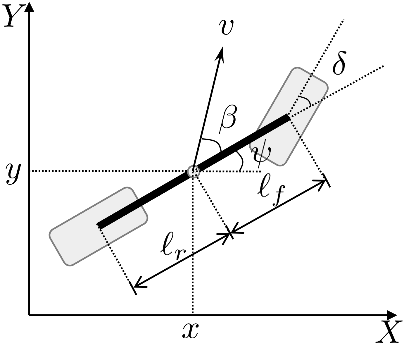
We consider a kinematic bicycle model (Fig. 2) in rajamani2011vehicle . The nonlinear continuous-time model is given as

	$\displaystyle\dot{x}$	$\displaystyle=v\cos(\psi+\beta)$
	$\displaystyle\dot{y}$	$\displaystyle=v\sin(\psi+\beta)$
	$\displaystyle\dot{\psi}$	$\displaystyle=\frac{v}{l_{r}}\sin(\beta)$
	$\displaystyle\dot{v}$	$\displaystyle=a$
	$\displaystyle\beta$	$\displaystyle=\arctan\Big{(}\frac{l_{r}}{l_{f}+l_{r}}\tan(\delta)\Big{)},$

where $x$ and $y$ are the coordinates of the center of mass, $v$ is the velocity of the center of mass, $\beta$ is the angle of the velocity $v$ with respect to the longitudinal axis of the vehicle, $a$ is the acceleration, $\psi$ is the heading angle of the vehicle, $\delta$ is the steering angle of the front wheel, and $l_{f}$ and $l_{r}$ represent the distance from the center of mass of the vehicle to the front and rear axles, respectively.

Since the proposed algorithm is for linear discrete-time systems, we perform the linearization and discretization as in law2018robust with sampling time $T_{s}=0.01s$ . We rewrite the system in the form of (3), where ${\bm{x}}_{k}=[x_{k},y_{k},\psi_{k},v_{k}]^{\top}$ is the state vector, ${\bm{u}}_{k}=[\beta_{k}^{u},a_{k}^{u}]^{\top}=\Big{[}\arctan\Big{(}\frac{l_{r}}{l_{f}+l_{r}}\tan(\delta_{k}^{u})\Big{)},a_{k}^{u}\Big{]}^{\top}$ is the input vector, and ${\bm{d}}_{k}=[\beta_{k}^{d},a_{k}^{d}]^{\top}=\Big{[}\arctan\Big{(}\frac{l_{r}}{l_{f}+l_{r}}\tan(\delta_{k}^{d})\Big{)},a_{k}^{d}\Big{]}^{\top}$ is the attack input vector. We consider the scenario that attack input is injected into the input, i.e. ${\bm{G}}_{k}={\bm{B}}_{k}$ . The system matrices are given as follows:

\displaystyle{\bm{A}}_{k}=\begin{bmatrix}1&0&0&T_{s}\\ 0&1&v_{k}T_{s}&0\\ 0&0&1&0\\ 0&0&0&1\end{bmatrix},\ {\bm{B}}_{k}={\bm{G}}_{k}=\begin{bmatrix}0&0\\ v_{k}T_{s}&0\\ \frac{v_{k}T_{s}}{l_{r}}&0\\ 0&T_{s}\end{bmatrix},

and ${\bm{C}}_{k}={\bm{I}}$ . The noise covariances ${\bm{Q}}_{k}$ and ${\bm{R}}_{k}$ are considered as diagonal matrices with $\operatorname*{\textit{diag}}({\bm{Q}}_{k})=[0.1,0.1,0.001,0.0001]$ and $\operatorname*{\textit{diag}}({\bm{R}}_{k})=[0.01,0.01,0.001,0.00001]$ .

The vehicle is assumed to have state constraints on the location $0\leq x_{k}\leq 20$ , $0\leq y_{k}\leq 5$ and the velocity $0\leq v_{k}\leq 22$ , and input constraints on the steering angle $|\delta|\leq 1.0472$ and the acceleration $|a|\leq 3.5$ .

The unknown attack signals are

	$\displaystyle\delta_{k}^{d}$	$\displaystyle=\begin{cases}0,&0\leq k<100\\ 1.1\sin(0.05k),&0\leq k<100\end{cases}$
	$\displaystyle a_{k}^{d}$	$\displaystyle=\begin{cases}0&0\leq k<100\\ 3.5,&100n\leq k<100(n+1)\\ -3.5,&100(n+1)\leq k<100(n+2)\end{cases},$

where $n=1,2,\cdots,5$ .

The constraints on the vehicle can be formulated by inequality constraints as in (4):

	$\displaystyle\underbrace{\begin{bmatrix}1&0\\ -1&0\\ 0&1\\ 0&-1\end{bmatrix}}_{\mathcal{A}_{k-1}}\begin{bmatrix}\delta_{k-1}^{d}\\ a_{k-1}^{d}\end{bmatrix}$	$\displaystyle\leq\underbrace{\begin{bmatrix}1.0472-\delta_{k-1}^{u}\\ 1.0472+\delta_{k-1}^{u}\\ 3.5-a_{k-1}^{u}\\ 3.5+a_{k-1}^{u}\end{bmatrix}}_{{\bm{b}}_{k-1}}$
	$\displaystyle\underbrace{\begin{bmatrix}1&0&0&0\\ -1&0&0&0\\ 0&1&0&0\\ 0&-1&0&0\\ 0&0&0&1\\ 0&0&0&-1\end{bmatrix}}_{\mathcal{B}_{k}}\begin{bmatrix}x_{k}\\ y_{k}\\ \psi_{k}\\ v_{k}\end{bmatrix}$	$\displaystyle\leq\underbrace{\begin{bmatrix}20\\ 0\\ 5\\ 0\\ 22\\ 0\end{bmatrix}}_{{\bm{c}}_{k}}.$

To reduce the effect of instantaneous noises, the cumulative sum algorithm (CUSUM) is adopted lai1995sequential . The $\chi^{2}$ test is utilized in a cumulative form. The $\chi^{2}$ CUSUM detector is characterized by the detector state $S_{k}\in\mathbb{R}_{+}$ :

\displaystyle S_{k}=\phi S_{k-1}+\hat{\bm{d}}_{k}^{\top}\bm{P}_{k}^{-1}\hat{\bm{d}}_{k},\quad S_{0}=0,

(55)

where $0<\phi<1$ is the pre-determined forgetting rate. At each time $k$ , the CUSUM detector (55) is used to update the detector state $S_{k}$ and detect the attack. In particular, we conclude that the attack is presented if

\displaystyle S_{k}>\sum_{i=0}^{\infty}\phi^{i}\chi^{2}_{df}(\alpha)=\frac{\chi^{2}_{df}(\alpha)}{1-\phi}.

(56)

All values are in standard SI units: $m$ (meter) for $l_{f}$ , $l_{r}$ , $x_{k}$ , and $y_{k}$ ; $rad$ for $\delta^{u}_{k}$ , $\delta^{d}_{k}$ , $\beta^{u}_{k}$ , $\beta^{d}_{k}$ , and $\psi_{k}$ ; $m/s$ for $v_{k}$ ; $m/s^{2}$ for $a^{u}_{k}$ and $a^{d}_{k}$ .

5.2 Results

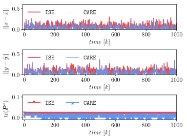
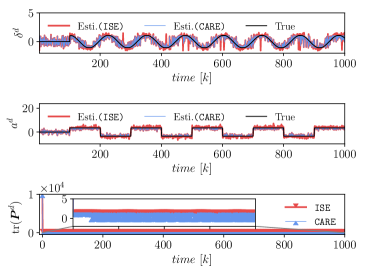
We show a comparison of the proposed algorithm (CARE) and the unified linear input and state estimator (ISE) introduced in yong2016unified . Figure 3 shows the estimation errors of the constrained states ( $x_{k}$ and $y_{k}$ ) and the traces of the state error covariances, and Fig. 4 shows the unknown attack signals and their estimates and traces of the attack estimation error covariances. As expected, CARE produces smaller state estimation error and lower covariance. When the attack happens after $k=100$ , the estimates obtained by CARE are closer to the true values and have lower error covariances (cf. Table 1).

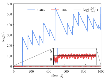
The estimates are used to calculate the detector state $S_{k}$ in (55). The statistical significance of the attack is tested using the CUSUM detector. The threshold is calculated by $\chi^{2}_{df}/(1-\phi)$ in (56) with the significance level $\alpha=0.01$ and the forgetting rate $\phi=0.15$ . The detector states and the threshold are plotted in $log-$ scale (Fig. 5). When the attack is present, CARE can detect the attack by producing high detector state values above the threshold, while the detector state values from ISE are oscillating around the threshold, suffering from a high false negative rate of $66.44\%$ .

6 Conclusion

In this paper, we presented a constrained attack-resilient estimation algorithm (CARE) of linear stochastic cyber-physical systems. The proposed algorithm produces minimum-variance unbiased estimates and utilizes physical constraints and operational limitations to improve estimation accuracy and detection performance via projection. In particular, CARE first provides minimum-variance unbiased estimates, and then these estimates are projected onto the constrained space. We formally proved that estimation errors and their covariances from CARE are less than those from unconstrained algorithms and showed that CARE had improved false negative rate in attack detection. Moreover, we proved that the estimation errors of the proposed estimation algorithm are practically exponentially stable. A simulation of attacks on a vehicle demonstrates the effectiveness of the proposed algorithm and reveals better attack-resilient properties compared to an existing algorithm.

Appendix A Gauss-Markov Theorem

Theorem 16 (Gauss-Markov Theorem sayed2003fundamentals )

Given the linear model ${\bm{y}}={\bm{H}}{\bm{x}}+{\bm{v}}$ , where ${\bm{v}}$ is a zero-mean random variable with positive-definite covariance matrix ${\bm{R}}_{v}$ and ${\bm{H}}$ is full rank $m\times n$ matrix with $m\geq n$ , the minimum-variance-unbiased linear estimator of ${\bm{x}}$ given ${\bm{y}}$ is $\hat{{\bm{x}}}=({\bm{H}}^{*}{\bm{R}}_{v}^{-1}{\bm{H}})^{-1}{\bm{H}}^{*}{\bm{R}}_{v}^{-1}{\bm{y}}$ .

Acknowledgements

This work has been supported by the National Science Foundation (ECCS-1739732 and CMMI-1663460).

References

(1) R. Rajkumar, I. Lee, L. Sha, J. Stankovic, Cyber-physical systems: the next computing revolution, in: IEEE Design Automation Conference, 2010, pp. 731–736.
(2) A. A. Cárdenas, S. Amin, S. Sastry, Research challenges for the security of control systems., HotSec 5 (2008) 15.
(3) R. M. Lee, M. J. Assante, T. Conway, German steel mill cyber attack, Industrial Control Systems 30 (2014) 22.
(4) J. Slay, M. Miller, Lessons learned from the Maroochy water breach, in: Springer International Conference on Eritical Infrastructure Protection, 2007, pp. 73–82.
(5) S. Peterson, P. Faramarzi, Iran hijacked us drone, says iranian engineer, Christian Science Monitor 15 (2011).
(6) K. Koscher, A. Czeskis, F. Roesner, S. Patel, T. Kohno, S. Checkoway, D. McCoy, B. Kantor, D. Anderson, H. Shacham, et al., Experimental security analysis of a modern automobile, in: IEEE Symposium on Security and Privacy, 2010, pp. 447–462.
(7) S. Checkoway, D. McCoy, B. Kantor, D. Anderson, H. Shacham, et al., Comprehensive experimental analyses of automotive attack surfaces, in: USENIX Security Symposium, Vol. 4, 2011, pp. 447–462.
(8) J. Raiyn, A survey of cyber attack detection strategies, International Journal of Security and Its Applications 8 (1) (2014) 247–256.
(9) A. A. Cardenas, S. Amin, S. Sastry, Secure control: Towards survivable cyber-physical systems, in: 28th International Conference on Distributed Computing Systems Workshops, 2008, pp. 495–500.
(10) F. Pasqualetti, F. Dörfler, F. Bullo, Attack detection and identification in cyber-physical systems, IEEE Transactions on Automatic Control 58 (11) (2013) 2715–2729.
(11) A. Teixeira, D. Pérez, H. Sandberg, K. H. Johansson, Attack models and scenarios for networked control systems, in: Proceedings of the 1st international conference on High Confidence Networked Systems, 2012, pp. 55–64.
(12) A. Teixeira, I. Shames, H. Sandberg, K. H. Johansson, A secure control framework for resource-limited adversaries, Automatica 51 (2015) 135–148.
(13) M. Pajic, J. Weimer, N. Bezzo, P. Tabuada, O. Sokolsky, I. Lee, G. J. Pappas, Robustness of attack-resilient state estimators, in: ACM/IEEE International Conference on Cyber-Physical Systems, 2014, pp. 163–174.
(14) H. Fawzi, P. Tabuada, S. Diggavi, Secure estimation and control for cyber-physical systems under adversarial attacks, IEEE Transactions on Automatic Control 59 (6) (2014) 1454–1467.
(15) M. Pajic, I. Lee, G. J. Pappas, Attack-resilient state estimation for noisy dynamical systems, IEEE Transactions on Control of Network Systems 4 (1) (2017) 82–92.
(16) M. Naghnaeian, N. H. Hirzallah, P. G. Voulgaris, Security via multirate control in cyber–physical systems, Systems & Control Letters 124 (2019) 12–18.
(17) N. H. Hirzallah, P. G. Voulgaris, N. Hovakimyan, On the estimation of signal attacks: A dual rate SD control framework, in: IEEE European Control Conference (ECC), 2019, pp. 4380–4385.
(18) Y. Liu, P. Ning, M. K. Reiter, False data injection attacks against state estimation in electric power grids, ACM Transactions on Information and System Security 14 (1) (2011) 21–32.
(19) Y. Mo, B. Sinopoli, Secure control against replay attacks, in: 47th Annual Allerton Conference on Communication, Control, and Computing, 2009, pp. 911–918.
(20) Y. Mo, R. Chabukswar, B. Sinopoli, Detecting integrity attacks on SCADA systems, IEEE Transactions on Control Systems Technology 22 (4) (2014) 1396–1407.
(21) S. Z. Yong, M. Zhu, E. Frazzoli, Resilient state estimation against switching attacks on stochastic cyber-physical systems, in: IEEE Conference on Decision and Control (CDC), 2015, pp. 5162–5169.
(22) N. Forti, G. Battistelli, L. Chisci, B. Sinopoli, A Bayesian approach to joint attack detection and resilient state estimation, in: IEEE Conference on Decision and Control (CDC), 2016, pp. 1192–1198.
(23) H. Kim, P. Guo, M. Zhu, P. Liu, Simultaneous input and state estimation for stochastic nonlinear systems with additive unknown inputs, Automatica 111 (2020) 108588.
(24) A. Teixeira, S. Amin, H. Sandberg, K. H. Johansson, S. S. Sastry, Cyber security analysis of state estimators in electric power systems, in: IEEE Conference on Decision and Control (CDC), 2010, pp. 5991–5998.
(25) D. Simon, T. L. Chia, Kalman filtering with state equality constraints, IEEE Transactions on Aerospace and Electronic Systems 38 (1) (2002) 128–136.
(26) S. Ko, R. R. Bitmead, State estimation for linear systems with state equality constraints, Automatica 43 (8) (2007) 1363–1368.
(27) D. Simon, Kalman filtering with state constraints: A survey of linear and nonlinear algorithms, IET Control Theory & Applications 4 (8) (2010) 1303–1318.
(28) H. Kong, M. Shan, S. Sukkarieh, T. Chen, W. X. Zheng, Kalman filtering under unknown inputs and norm constraints, Automatica 133 (2021) 109871.
(29) A. I. Mourikis, S. I. Roumeliotis, A multi-state constraint Kalman filter for vision-aided inertial navigation, in: IEEE International Conference on Robotics and Automation (ICRA), 2007, pp. 3565–3572.
(30) L. Wang, Y. Chiang, F. Chang, Filtering method for nonlinear systems with constraints, IEEE Proceedings-Control Theory and Applications 149 (6) (2002) 525–531.
(31) S. Z. Yong, M. Zhu, E. Frazzoli, Simultaneous input and state estimation of linear discrete-time stochastic systems with input aggregate information, in: IEEE Conference on Decision and Control (CDC), 2015, pp. 461–467.
(32) S. H. Kafash, J. Giraldo, C. Murguia, A. A. Cardenas, J. Ruths, Constraining attacker capabilities through actuator saturation, in: IEEE American Control Conference (ACC), 2018, pp. 986–991.
(33) S. M. Djouadi, A. M. Melin, E. M. Ferragut, J. A. Laska, J. Dong, A. Drira, Finite energy and bounded actuator attacks on cyber-physical systems, in: IEEE European Control Conference (ECC), 2015, pp. 3659–3664.
(34) S. Z. Yong, M. Zhu, E. Frazzoli, A unified filter for simultaneous input and state estimation of linear discrete-time stochastic systems, Automatica 63 (2016) 321–329.
(35) H. Kim, P. Guo, M. Zhu, P. Liu, Attack-resilient estimation of switched nonlinear cyber-physical systems, in: IEEE American Control Conference (ACC), 2017, pp. 4328–4333.
(36) P. Guo, H. Kim, N. Virani, J. Xu, M. Zhu, P. Liu, Roboads: Anomaly detection against sensor and actuator misbehaviors in mobile robots, in: 48th Annual IEEE/IFIP international conference on dependable systems and networks (DSN), 2018, pp. 574–585.
(37) B. O. Teixeira, J. Chandrasekar, L. A. Tôrres, L. A. Aguirre, D. S. Bernstein, State estimation for linear and non-linear equality-constrained systems, International Journal of Control 82 (5) (2009) 918–936.
(38) B. D. O. Anderson, J. B. Moore, Detectability and stabilizability of time-varying discrete-time linear-systems, SIAM Journal on Control and Optimization 19 (1) (1981) 20–32.
(39) S. Kluge, K. Reif, M. Brokate, Stochastic stability of the extended Kalman filter with intermittent observations, IEEE Transactions on Automatic Control 55 (2) (2010) 514–518.
(40) A. Papoulis, S. U. Pillai, Probability, random variables, and stochastic processes, Tata McGraw-Hill Education, 2002.
(41) D. J. Tylavsky, G. R. Sohie, Generalization of the matrix inversion lemma, Proceedings of the IEEE 74 (7) (1986) 1050–1052.
(42) R. Rajamani, Vehicle dynamics and control, Springer Science & Business Media, 2011.
(43) C. K. Law, D. Dalal, S. Shearrow, Robust model predictive control for autonomous vehicles/self driving cars, arXiv preprint arXiv:1805.08551 (2018).
(44) T. L. Lai, Sequential changepoint detection in quality control and dynamical systems, Journal of the Royal Statistical Society. Series B (Methodological) (1995) 613–658.
(45) A. H. Sayed, Fundamentals of adaptive filtering, John Wiley & Sons, 2003.

	$\displaystyle\\|{\bm{A}}_{k}\\|\leq\bar{a},$	$\displaystyle\\|{\bm{C}}_{k}\\|\leq\bar{c}_{y},$	$\displaystyle\\|{\bm{G}}_{k}\\|\leq\bar{g},$
	$\displaystyle\\|{\bm{M}}_{k}\\|\leq\bar{m},$	$\displaystyle{\bm{Q}}_{k}\geq\underaccent{\bar}{q}{\bm{I}}.$

	$\displaystyle\mathbb{E}[\\|\tilde{{\bm{x}}}_{k}\\|^{2}]$	$\displaystyle\leq a_{x}e^{-b_{x}k}\mathbb{E}[\\|\tilde{{\bm{x}}}_{0}\\|^{2}]+c_{x}$
	$\displaystyle\mathbb{E}[\\|\tilde{{\bm{d}}}_{k}\\|^{2}]$	$\displaystyle\leq a_{d}e^{-b_{d}k}\mathbb{E}[\\|\tilde{{\bm{d}}}_{0}\\|^{2}]+c_{d}.$

Constrained Attack-Resilient Estimation of Stochastic Cyber-Physical Systems

Abstract

keywords:

1 Introduction

Related work

Contributions

Paper organization

2 Preliminaries

Notations

χ2\chi^{2} Test for Detection

False negative rate

Problem Formulation

Remark 1

Problem statement

3 Algorithm Design

3.1 Algorithm Statement

3.2 Algorithm Derivation

Prediction

Attack estimation

Proposition 2

Proposition 3

Remark 4

Time update

Measurement update

Projection update

4 Performance and Stability Analysis

4.1 Performance Analysis

Lemma 5

Theorem 6

Assumption 7

Remark 8

Theorem 9

4.2 Stability Analysis

Assumption 10

Remark 11

Theorem 12

Theorem 13

Claim 14

Claim 15

5 Illustrative Example

5.1 Experimental Setup

5.2 Results

6 Conclusion

Appendix A Gauss-Markov Theorem

Theorem 16 (Gauss-Markov Theorem sayed2003fundamentals )

Acknowledgements

References

$\chi^{2}$ Test for Detection