QCDSF/UKQCD/CSSM Collaboration
Constraining beyond the Standard Model nucleon isovector charges
Abstract
At the TeV scale, low-energy precision observations of neutron characteristics provide unique probes of novel physics. Precision studies of neutron decay observables are susceptible to beyond the Standard Model (BSM) tensor and scalar interactions, while the neutron electric dipole moment, , also has high sensitivity to new BSM CP-violating interactions. To fully utilise the potential of future experimental neutron physics programs, matrix elements of appropriate low-energy effective operators within neutron states must be precisely calculated. We present results from the QCDSF/UKQCD/CSSM collaboration for the isovector charges and of the nucleon, and baryons using lattice QCD methods and the Feynman-Hellmann theorem. We use a flavour symmetry breaking method to systematically approach the physical quark mass using ensembles that span five lattice spacings and multiple volumes. We extend this existing flavour breaking expansion to also account for lattice spacing and finite volume effects in order to quantify all systematic uncertainties. Our final estimates of the nucleon isovector charges are and renormalised, where appropriate, at in the scheme.
I Introduction
Historically nuclear and neutron beta decays have played an important role in determining the vector-axial (V-A) structure of weak interactions and in shaping the Standard Model (SM). However, more recently, neutron and nuclear -decays can also be used to probe the existence of beyond the Standard Model (BSM) tensor and scalar interactions. The interaction of the boson with the neutron and proton during neutron -decay is proportional to the matrix element of flavour changing vector and axial-vector currents between the initial neutron state and final proton state, with coupling constants [1]. It has been identified that the potential existence of BSM tensor and scalar couplings would provide additional contributions to neutron -decay [2]. These new BSM contributions are proportional to analogous matrix elements of flavour-changing tensor or scalar operators. To gain sensitivity to these effects the majority of previous and proposed neutron beta decay studies aim to determine one or more of the correlation coefficients included in the differential decay rate for a beam of polarised neutrons [2]:
| (1) | ||||
where is the neutron spin, is the momentum of the electron and is the momentum of the neutrino with energies and , respectively, and is the end-point energy of the electron. In the SM, , where is the ratio of the axial-vector and vector coupling constants and is the Fermi constant. The neutron decay observables include, , the neutrino-electron correlation coefficient, , the Fierz interference term, , the beta asymmetry, and , the neutrino asymmetry. Within the SM, the correlation coefficients and depend solely on the ratio of the axial-vector and vector coupling constants, . However the parameter, , is included to account for the case of the hypothetical scalar or tensor couplings in addition to the (V-A) interaction of the SM. Many experiments are underway worldwide with the aim to improve the precision of measurements of these neutron decay observables, two importantly being the neutrino asymmetry [3], and the Fierz interference term [4, 5]. The parameter has linear sensitivity to BSM physics through [6]:
| (2) | ||||
| (3) | ||||
where and are the new-physics effective couplings and and are the tensor and scalar nucleon isovector charges. Here is a correction term to the neutrino asymmetry correlation coefficient, , and is an addition to the Fierz interference term in Eq. 1. Data taken at the Large Hadron Collider (LHC) is currently looking at probing scalar and tensor interactions at the level [7]. However to fully assess the discovery potential of experiments at the level it is crucial to identify existing constraints on new scalar and tensor operators.
Another quantity of interest is the neutron electric dipole moment (EDM), which is a measure for CP violation. In extensions of the Standard Model quarks acquire an EDM through the interaction of the photon with the tensor current [8]. The contribution of the quark EDMs, , to the EDM of the neutron, , is related to the quark tensor charges, , by [9, 10, 11]:
| (4) |
Here are the new effective couplings which contain new CP violating interactions at the TeV scale. The current experimental data gives an upper limit on the neutron EDM of .cm [12]. In calculating the tensor charges and knowing a bound on , we are able to constrain the couplings, , and hence BSM theories.
In recent years there has been an increase in interest from lattice QCD collaborations in calculating the axial, scalar and tensor isovector charges due to their importance in interpreting the results of many experiments and phenomena mediated by weak interactions [13, 14, 15, 16, 17, 18, 19]. The QCDSF/UKQCD/CSSM collaborations have an ongoing program investigating various hadronic properties using the Feynman-Hellmann theorem [20, 21, 22, 23, 24, 25, 26, 27]. Here we extend this work to a dedicated study of the nucleon tensor, scalar and axial charges. We discuss a flavour symmetry breaking method to systematically approach the physical quark mass. We then extend this existing flavour breaking expansion to also account for lattice spacing and finite volume effects to quantify systemic uncertainties. Finally, we look at the potential impact of our results on measurements of the Fierz interference term and the neutron EDM.
II Simulation Details
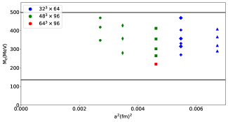
For this work we use gauge field configurations that have been generated with flavours of dynamical fermions, using the tree-level Symanzik improved gluon action and non-perturbatively improved Wilson fermions [28]. In our simulations, we have kept the bare average quark mass, , held fixed approximately at its physical value, while systematically varying the quark masses around the flavour symmetric point, , to extrapolate results to the physical point [29]. We also have degenerate and quark masses, . The coverage of lattice spacings and pion masses is represented graphically in Fig. 1.
| (fm) | Volume | (MeV) | |||
| * | |||||
| * | |||||
| * | |||||
Further information about these ensembles is presented in Table 1 and Appendix A, Table 7. We have five lattice spacings, fm [30], enabling an extrapolation to the continuum limit as well as three lattice volumes, , and , allowing an extension to the flavour-breaking expansion, which describes the quark mass-dependence of the matrix elements, to also account for lattice spacing and finite volume effects. We also use a bootstrapping resampling technique to compute all statistical uncertainties in our study.
In order to compare with existing results in the literature we use the renormalisation constants given in Table 2. Table 2 summarises the renormalisation constants at each value of after chiral and continuum extrapolation across multiple masses with conversion from R-MOM to at GeV. The renormalisation constants are calculated following the method in Ref. [32] and the results first appeared in Ref. [31].
III The Feynman-Hellmann Theorem
The Feynman-Hellmann (FH) theorem is used to calculate hadronic matrix elements in lattice QCD through modifications to the QCD Lagrangian. The expression for the FH theorem in the context of field theory is [20]:
| (5) |
where is a modified action of our theory so that it depends on some parameter , and is the energy of a hadron state, . This result relates the derivative of the total energy to the expectation value of the derivative of the action with respect to the same parameter.
III.1 Application and implementation
Consider the following modification to the action of our theory:
| (6) |
Then the FH theorem as shown in Eq. 5, provides a relationship between an energy shift and a matrix element of interest:
| (7) |
Importantly, the right-hand side is the standard matrix element of the operator inserted on the hadron, , in the absence of any background field. In lattice calculations, we modify the action in Eq. 6, then examine the behaviour of hadron energies as the parameter changes, and finally extract the above matrix element from the slope at .
In order to calculate the tensor, axial and scalar charges of a baryon, the extra terms we add to the QCD action are:
| (8) | ||||
| (9) | ||||
| (10) |
where we will take the case of each quark flavour, , separately, , are the phase factors and there are four choices of and . The phase factors chosen here are , and , . The tensor, axial and scalar charges are related to the baryon matrix elements of the same operators:
| (11) | ||||
where , and [33]. In our simulations, we have chosen , and :
| (12) | ||||
where, , is the spin of the baryon polarised in the direction.111Our spin vector is given by , where , with quantisation axis where , and . For our case we have , , and . Therefore , and . Hence the FH theorem in Eq. 7 for the tensor and axial charges gives:
| (13) |
where we have dropped the, , subscript as from now on we are only dealing with baryon states and denotes the baryon energy with spin up/down in the direction in the presence of a tensor or axial background field (Eq. 8 and Eq. 9) with strength . For small values of , the energy is therefore given by:
| (14) |
We have related the change in energy of the hadron state to the spin contribution from the quark flavour . Alternatively, due to the combination of , the spin-down state with positive is equivalent to the energy shift of the spin-up state with negative . For the scalar we simply have:
| (15) | ||||
Here the insertion is on the quark flavour . For example, we use the perturbed propagator for the -quark in the proton to get the -quark contribution to the nucleon isovector charge. The nucleon isovector charges are then given by the difference between the up and down quark contributions:
| (16) |
Here we only insert the operator into the propagators used in the quark-line connected contributions; there are no quark-line disconnected terms considered here as they cancel in the case . To improve the precision of our results we can take advantage of the fact that we are only interested in energy changes due to changes in , specifically the change in energy around the point , with respect to the unperturbed energy. We consider two correlation functions, one calculated at and the other at some finite value of . If we take the ratio of these two quantities, we find:
| (17) |
The exponential dependence on now contains the difference in energies between the unperturbed energy and the energy at some .
and are both measured on the same configurations, so both will have correlated noise. Using this ratio to determine energy differences has the advantage that the noise will largely cancel, leaving to a more reliable energy shift. We can also constrain our fit function to pass through zero by construction as there is no difference in energies at .
The extraction of hadron matrix elements in lattice QCD demands careful attention to contamination from excited states. Excited-state contamination has an impact on the study of standard baryon three-point functions due to the presence of weak signal-to-noise behavior at large Euclidean times. Various techniques are used to address excited-state contamination, one of which is the variational method. The variational method has been widely successful in spectroscopy investigations [34, 35, 36, 37, 38, 39, 40], and has also found application in the analysis of hadronic matrix elements [41, 42, 43, 44, 45, 46]. Another popular method is the “two-exponential fit” and “summation” methods seen in Refs. [45, 46, 47, 48, 49, 50, 51]. A summary of these methods as well as a comparison between them can be seen in Ref. [52].
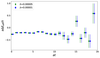
Since in this investigation hadron energies are extracted from two-point functions, control of excited state contamination in the Feynman-Hellmann is simplified compared to standard three-point analyses. For example Fig. 2 shows the effective energy shift for the ratio (Eq. 17) divided by for the down quark at two different values of . In Fig. 2 we see a plateau in the effective mass indicating a clear region where the ground state can be isolated.
IV Weighted Averaging Method
The dependency of the fits on the time ranges used is a source of systematic uncertainty. To address these issues, we use a weighted averaging method on the fit results to limit the impact of the fit window selection. The weighted averaging method we use is a simplified variation of that outlined in detail in Ref. [53] and has similarities to that proposed in Ref. [54]. We proceed by determining the energy shifts, , by fitting the ratio of perturbed to unperturbed correlation functions using Eq. 17 for a variety of different Euclidean time fit windows. The largest time slice employed in each fit for each ensemble and operator is fixed to be the last time slice before the signal is lost due to statistical noise. For example, in Fig. 2 this would be chosen to be . The start of the fit range, , is varied between for ensembles with respectively and up to the largest value of such that no less than four time slices are used in a fit. By adjusting the minimum time of the fit range, , based on the lattice spacing of each ensemble, we are ensuring that each fit starts at an earlier scale. In the following we refer to the value of for a single fit, , as . Each fit result is then assigned a weight:
| (18) |
where labels the choice of fit range specified by for a fixed , is the p-value of the fit and is the uncertainty in the energy shift, , for fit . Taking a weighted average of the fit findings, , provides the final estimate of the energy shift, , and associated uncertainty ,
| (19) | ||||
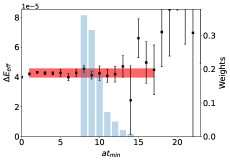
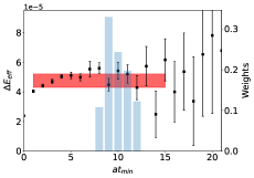
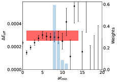
The total error describes the combined statistical uncertainty on plus the systematic uncertainty arising from the choice of fit range. The separating of this error into and only partially separates statistical and systematic uncertainties because includes statistical errors plus systematic uncertainties related to fluctuations among the . The final estimate, , provides an estimate of the energy of the hadron with reduced systematic bias arising from choice of fit window. Fig. 3 shows the proton effective energy shift for the ratio (Eq. 17), using the standard definition of an effective mass. The final estimate of the energy shift, , when using the weighted averaging method is indicated by the red band. Fig. 3 also includes a bar graph for the weights assigned to each fit value.
V Determination of Matrix Elements
V.1 Feynman-Hellman Method
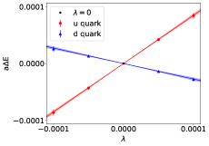
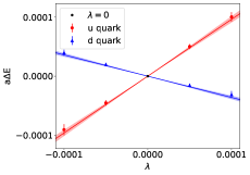
Now that we have a procedure for reliably determining the energy shifts, we are now in a position to determine at multiple values of for a fixed ensemble and operator. In Fig. 4 we plot the calculated proton energy shifts for each value of for the fm ensemble with . Fig. 4(a) shows results for the tensor operator, while Fig. 4(b) shows those for the axial operator. Now performing a linear fit to Eq. 14 and extracting the slope we obtain the following results,
, , and , with the tensor results, renormalised at in the scheme using the renormalisation factors given in Table 2.
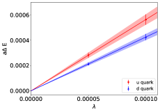
Similarly for the scalar charge, in Fig. 4(c) we perform a linear fit to Eq. 15 and by extracting the slope we find, and , again renormalised at in the scheme. The above process has been repeated for all quark masses on each of the lattice spacings as well as for the and baryons. The results can been found in Appendix B, in Tables 8, 9, 10.
V.2 Two-exponential fit method
Here we compare the FH method results to the popular “two-exponential fit” method using three point functions. This is undertaken by expanding the two-point and three-point functions to the second energy state and fitting to obtain the parameters of interest. The process for the two-exponential fit is to fit the two-point correlator over a sink time range in which the two-state initial fit assumption is justified. Then using these extracted parameters in the fit to the three-point correlator using a range that also satisfies a two-state initial fit assumption. A detailed treatment of the two-exponential fit is given in, for example, Ref. [52].
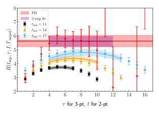
Fig. 5 shows a comparison of the result for extracted using the FH method (red band) and the result using the two-exponential fit method (purple band). The red points come from a fixed value, similar to that shown in Fig. 2, whereas the red band comes from performing a linear fit to Eq. 14 and extracting the slope. We can see that the results using the FH method is in excellent agreement with the standard three-point analysis.
Now that we have the quark contributions for multiple lattice ensembles, in the next section we shall use a flavour symmetry breaking method to extrapolate results for the nucleon isovector charges to the physical quark mass.
VI Flavour Symmetry Breaking
The QCD interaction is flavour-blind, which means that the only distinction between quark flavours comes from the quark masses when we disregard the electromagnetic and weak interactions. The theory behind these interactions is easiest to understand when all three quark flavours share the same mass, as this allows us to use the full power of flavour symmetry. Here we have kept the bare quark mass, , held fixed at its physical value, while systematically varying the individual quark masses around the flavour symmetric point, , in order to constrain the extrapolation to the physical point. In this work we simulate with degenerate and quark masses , restricting ourselves to .
When is unbroken all octet baryon matrix elements of a given octet operator can be expressed in terms of just two couplings and . However, once is broken and we move away from the symmetric point we can construct quantities (, ) which are equal at the symmetric point but differ in the case where the quark masses are different. The theory behind constructing these quantities is described in detail in Ref. [55] and is summarised below. The result of constructing these quantities leads to ‘fan’ plots, with slope parameters (, ) relating them. Following the method in Ref. [55] we use the expansion to extrapolate the nucleon charges to the physical point.
In this work, we describe the quark mass dependence of the hadronic matrix elements by a perturbation in the quark masses about an symmetric point. This perturbation generates a polynomial expansion in the quark mass differences (i.e. the breaking parameter) and therefore appears distinct from a chiral formulation that generates nonanalytic behaviour (e.g. logarithms) in the vicinity of the 2- or 3-flavour chiral limits. However, it has been demonstrated in Ref. [56], that by expanding the logarithmic features about a fixed quark mass point (such as the chosen symmetric point), the infrared singularities reveal themselves in the high-order terms of the polynomial expansion — hence demonstrating that the group-theoretic expansion does encode the same physics that appears in the logarithms. A detailed numerical investigation exploring the numerical convergence from both limits goes beyond the present work. Here we assess the convergence of our expansion empirically, subject to the precision of our numerical results.
VI.1 Mass dependence of amplitudes
In order to find the allowed mass dependence of the octet operators in hadrons we need the decomposition of the . singlet and octet coefficients are constructed through group theory and using a mass Taylor expansion, which can be seen in Ref. [55]. Here we summarise the coefficients in Table 3.
| , class | , class | |||||||
|---|---|---|---|---|---|---|---|---|
| f | d | d | d | d | f | f | ||
| I | f | d | ||||||
| 0 | -1 | 1 | 0 | 0 | 0 | -1 | ||
| 0 | 0 | 2 | 1 | 0 | 2 | 0 | 0 | |
| 0 | 0 | -2 | 1 | 2 | 0 | 0 | 0 | |
| 0 | - | -1 | 1 | 0 | 0 | 0 | 1 | |
| 1 | 1 | 0 | 0 | -2 | 2 | 0 | ||
| 1 | 2 | 0 | 0 | 0 | 0 | -2 | ||
| 1 | 1 | - | 0 | 0 | 2 | 2 | 0 | |
These coefficients are used to construct equations which are linear in , where:
| (20) |
is the difference of the light quark mass to the symmetric point. Using the definitions in Table 4, we introduce the notation for the matrix element transition of as follows:
| (21) |
| Index | Baryon () | Meson () | Current () |
|---|---|---|---|
| 1 | |||
| 2 | |||
| 3 | |||
| 4 | |||
| 5 | |||
| 6 | |||
| 7 | |||
| 8 | |||
| 0 |
where is the appropriate operator, or current, from Table 4 and represents the flavour structure of the operator. From Table 3 we can now read off the expansions of the various matrix elements, where the and terms are independent of and the coefficients , , and , are the leading order terms. For example if we look at the term, we have to first order in :
| (22) |
VI.2 Mass Dependence: ‘Fan Plots’
Since we hold the average quark mass, , fixed, while moving away from the symmetric point, we only need to consider the non-singlet polynomials in the quark mass. In this sub-section quantities are constructed which are equal at the symmetric point and differ in the case where the quark masses are different. We can then evaluate the the violation of symmetry that emerges from the difference in .
VI.2.1 The d-fan
Following Ref. [55], we construct the following combinations of matrix elements which have the same value, , at the symmetric point:
| (23) | ||||
By constructing these quantities the result is a ‘fan’ plot with seven lines and three slope parameters and constraining them. The slope parameters can be constrained by calculating octet baryon matrix elements on a set of ensembles with varying quark masses at fixed lattice spacing, such as those given in Table 1, and constructing the s. For the forward matrix elements considered here, these s can also be written as linear combinations of the different quark contributions to the baryon charges. For example, using Table 4 we see:
| (24) | ||||
where we introduce the notation to denote the quark, , contribution to the overall charge in the baryon, . In this work we only consider the flavour diagonal matrix terms, i.e. there are no transition terms. Therefore, only the diagonal terms, , and , are used. An ‘average D’ can also be constructed from the diagonal amplitudes:
| (25) |
which is constant in up to terms . When constructing these fan plots it is useful to plot to find the average fit to reduce statistical fluctuations.
VI.2.2 The f-fan
Similarly another five quantities, , can be constructed which all have the same value, , at the symmetric point:
| (26) | ||||
Again, an ‘average F’ can be calculated through:
| (27) |
In this work, only the connected quark-line terms are computed. Quark-line disconnected terms only show up in the coefficient and cancels in the case . Unlike the -fan, the -fan to linear order, has no error from dropping the quark-line disconnected contributions, as none of the parameters appear in the -fan.
VI.3 Fan Plot Results
Here we present results using the fm ensemble. Results from other lattice spacings are similar. In Section VII, we will extend this method to include all ensembles and present the final results for .
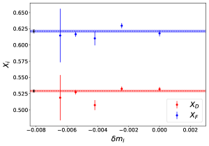
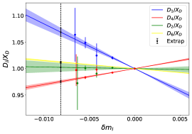
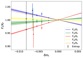
The singlet quantities and are calculated using Eq. 25 and Eq. 27. In Fig. 6 and are plotted against and fitted to a constant. Since in Section VII we will work to in our flavour-breaking expansions, we fit and to constants in order to determine their values at the physical quark masses. The constant fits to the fm data are shown by the dashed lines in Fig. 6. In Fig. 7(a) we present the D-‘fan’ plot which shows the dependence of the for and . Here the lines correspond to the linear in fits using Eq. LABEL:eqn:Dfan. From these linear fits the slope parameters and are determined. It is interesting to note that these parameters also lead to a prediction for the flavour off-diagonal term for , which is also shown. Similarly in Fig. 7(b) we present the F-‘fan’ plot for , and , where the lines correspond to the linear fits using Eq. LABEL:eqn:Ffan. Similarly, the parameters and are determined from the linear fits. Again, the corresponding off-diagonal terms for are also predicted and plotted. By forming appropriate linear combinations, we reconstruct the matrix elements for an individual quark flavour in a particular hadron:
| (28) | ||||
and hence the nucleon isovector charges can be determined:
| (29) |
for and . To obtain an extrapolation of to the physical point, we evaluate the expressions in Eq. 28 at and substitute in the estimated values for and . In order to quantify systemic uncertainties we will now extend this flavour breaking expansion method further.
VII Global Fits
The flavour breaking expansion described in Section VI only accounts for the quark mass-dependence of the matrix elements. However, in order to quantify systematic uncertainties, here we extend this method to also account for lattice spacing, finite volume effects and second order mass terms. As we are performing a global fit over all ensembles, we are now able to place constraints on the second-order mass terms, which means that all fits will now incorporate a term of order . These fits also include corrections with respect to , and . In order to perform a global fit across all masses we substitute the quantity from here on with:
| (30) |
where the pseudoscalar mass flavour singlet, , is given by:
| (31) |
By determining to now be dimensionless and given in terms of physical quantities we are now able to combine results from different lattice spacings. The fit used for the singlet quantities and are extended to [56]:
| (32) | ||||
where we also consider an alternative lattice spacing dependence by replacing with . The term estimates the finite size effects, where the leading meson-loop contribution has the functional form [57]:
| (33) |
It is important to note that here finite size effects are only included in the singlet quantities and and not in the and fan plot fits as the finite size corrections to the flavour-breaking coefficients determined by fits to, e.g. are expected to be sub-dominant compared to those in the corresponding singlet quantities. The fits used for the fan, , are of the form:
| (34) | ||||
and similarly for the fan, :
| (35) | ||||
| Fit | D-Fan | F-Fan | ||||||
|---|---|---|---|---|---|---|---|---|
| 1. | ||||||||
| 2. | ||||||||
| 3. | ||||||||
| 4. | ||||||||
| 5. | ||||||||
| 6. | ||||||||
| Fit | D-Fan | F-Fan | ||||||
| 1. | ||||||||
| 2. | ||||||||
| 3. | ||||||||
| 4. | ||||||||
| 5. | ||||||||
| 6. | ||||||||
| Fit | D-Fan | F-Fan | ||||||
| 1. | ||||||||
| 2. | ||||||||
| 3. | ||||||||
| 4. | ||||||||
| 5. | ||||||||
| 6. |
The coefficients were computed for the EM form factors in Ref. [55]. At there are 12 amplitudes and 11 coefficients so there is just one constraint. However, here we only consider the diagonal amplitudes and therefore we do not have 12 amplitudes and hence they are unable to be constrained here [59]. Therefore they are replaced with one coefficient () for each and .
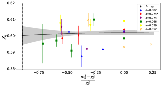
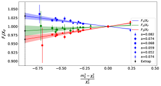
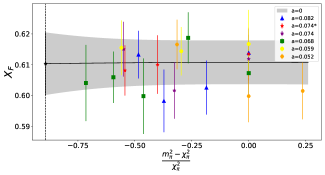
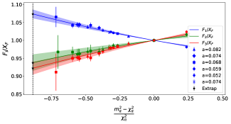
Now we perform a combination of different fits summarised in Table 5. Firstly, the fit is performed individually on and . An example of this is shown in Fig. 8(a) and (c). In Fig 8(a) we show as a function for ‘Fit 1’, which only includes the constant term, and a term in Eq. 32, while Fig 8(c) shows as a function of with the result from using Eq. 32 with all corrections included (‘Fit 4’). The extrapolated result for and are summarised in Table 5 taken in the limits , and physical masses. Similarly, fits are performed on the fan plots using Eq. LABEL:eqn:Dfan_gf and Eq. LABEL:eqn:Ffan_gf. Fig. 8(b) and (d) shows the results when using ‘Fit 1’ and ‘Fit 4’, where it is important to mention that all data points are shifted in the limit in Figs. 8(c)(d). The slope results are then multiplied by the extrapolated results for and :
| (36) | ||||
The resulting slope parameters , and the coefficients are then included in the reconstruction of the matrix elements in a particular hadron:
| (37) | ||||
where and . The final result for are then given in the limit, , and is the physical mass. The final results for , and for each fit are summarised are in Table 5, together with the for each fit.
VII.1 Results
In order to combine these results we extend our weighted averaging method described in section IV. To do this we combine the and degrees of freedom of , , -fan and -fan; enumerated by , respectively, in the following:
| (38) |
where labels one of the six fit types. Each fit is then assigned a weight using the combined :
| (39) |
where is the -value of the fit and is the uncertainty in the nucleon isovector charges calculated using Eq. 37. Taking a weighted average of the six fit results, , provides a final estimate of the nucleon isovector charges, , and associated uncertainty:
| (40) | ||||
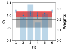
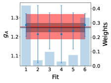
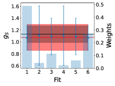
Fig. 9 shows the results for each fit and their assigned weight. The final estimate of the nucleon isovector charges, , renormalised using the results given in Table 2, at in the , are:
| (41) | ||||
| (42) | ||||
| (43) |
where the systematic errors labelled as ‘a’ and ‘FV’ represent the difference in the central value obtained by incorporating a lattice spacing correction compared to without, and likewise for the finite volume correction. These final results, with statistical and systematic errors combined in quadrature, are shown by the red bands in Fig. 9. We note our results for , and are all comparable with the FLAG Review results [58], represented by the grey bands in Fig. 9. Of particular note is that we have determined to the level. However, work is still needed in order reduce the uncertainties on, and , to understand it at the same level.
As a check on our method for combining the results from the six different fits given in Table 5, we employ the widely used Akaike Information Criterion (AIC). Here results obtained from the various fits are weighted using the Akaike weights [60]:
| (44) |
Akaike’s information criterion takes on the simple form for models with normally distributed errors:
| (45) |
where is the same as that calculated in Eq. 38 and is the number of parameters in each fit. As a result the AIC weight prefers the models with lower values, but penalises those with too many fit parameters. The above method was repeated using the AIC weights. This gives the following results for the nucleon isovector charges, , and , where the errors have been added in quadrature. These results are in agreement with those in Eq. 41, 42 and 43.
VII.2 Hyperons
Here we calculate flavour-diagonal matrix elements of hyperons using the same method. Ref. [61] demonstrates that isovector combinations of hyperon charges are relevant in searches for new physics through semileptonic hyperon decays. The calculated slope parameters , and the coefficients can also be used in the reconstruction of the matrix elements in a particular hyperon. The theory behind constructing these quantities is described in detail in Ref. [55] and is summarised in Appendix. C. The results for the charges of the and baryons are summarised in Table 6.
| Tensor | Axial | Scalar | |
|---|---|---|---|
To properly exploit the increased experimental sensitivity to hypothetical tensor and scalar interactions, we require lattice-QCD estimates of the nucleon isovector charge, at the level of [6]. The results presented here are at the level. As the overall goal of this research is to support precision tests of the Standard Model, we have successfully demonstrated the validity of our approach. We can now look at the effect this has on phenomenology.
VIII Impact of Lattice Results on Phenomenology
As discussed in Section I, it is expected that future neutron beta decay experiments will increase their sensitivity to BSM scalar and tensor interactions through improved measurements of the Fierz interference term, , as well as the neutrino asymmetry parameter, . In order to assess the full impact of these future experiments we have performed an analysis of the tensor charge and . Here we discuss existing constraints on new scalar and tensor couplings which arise from low-energy experiments. Finally, using the existing constraints on and as well as our calculated value for and , we determine the allowed regions in the plane.
VIII.1 Low-energy phenomenology of scalar and tensor interactions
VIII.1.1 transitions and scalar interactions
The most precise bound on the scalar coupling comes from nuclear beta decay. The differential decay rate for nuclear beta decay has coefficient and Fierz interference term [6]:
| (46) | ||||
| (47) |
where is the atomic number of the daughter nucleus. We can see from Eq. 47 that couples to the BSM scalar interaction. From a comparison of well known half-lives corrected by a phase-space factor, Hardy and Towner [62] found . This result was found using a number of daughter nuclei and averaging over the set. This can be converted to the following bound on the product of scalar charge and the new-physics effective scalar coupling:
| (48) |
This is the most precise bound on the scalar interactions from low-energy probes.
VIII.1.2 Radioactive Pion Decay and the Tensor Interaction
An analysis of radioactive pion decay is sensitive to the same tensor operator that can be investigated in beta decays. The experimental results from the PIBETA collaboration [63] put constraints on :
| (49) |
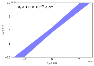
Currently this is the most stringent constraint on the tensor coupling from low energy experiments. Using these constraints, as well Eq. 2 and Eq. 3, bounds can be put on the new scalar and tensor interactions at the level. Following the work of Ref. [6], in Fig. 10 we show the constraint on the plane.
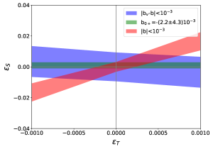
The current best constraints on scalar and tensor interactions arise from nuclear beta decays and radioactive pion decay, which is shown by the green band [6, 62]. The neutron constraints are future projections at the level, derived from Eq. 2 and Eq. 3, using the tensor and scalar charges as obtained in this work, shown by the red and blue bands in Fig. 10. When accounting for uncertainties in these lattice QCD calculations, the boundaries on the bands in Fig. 10 become wider and the bands take on a ‘bow-tie’ shape. However most of the constraining power is lost due to the large uncertainty in our value for . In order to fully utilise the constraining power of experiments, understanding the lattice-QCD estimates of the nucleon tensor and scalar charge at the level of is required [6]. We have successfully calculated the tensor charge at the level and are able to fully utilise the constraining power future experiments.
VIII.2 Quark electric dipole moment
In this section we briefly discuss the impact our results have on constraining the quark EDM couplings using the current bound on the neutron EDM. Using the same method followed in Section VII we are able to constrain . We note that in this work we have only considered quark-line connected contributions, although other works have shown the disconnected contributions to be small at near-physical quark masses [64]. This is in line with expectations based on the fact that the tensor operator is a helicity-flip operator and hence disconnected contributions mush vanish in the chiral limit. Using Eq. 37 we can calculate the up and down contributions to the nucleon tensor charge for each fit listed in Table 5. Applying the weighted averaging method, the final estimates for, , are:
| (50) | |||
| (51) |
IX Conclusion
In this work we have presented results for the axial, tensor and scalar nucleon and hyperon charges using the Feynman-Hellmann theorem, as well as using a flavour symmetry breaking method to systematically approach the physical quark masses. We applied a weighted averaging method on the fit results, removing possible systematic uncertainties which arise from a bias in choosing the fit windows. In the flavour symmetry breaking method, symmetry constraints are automatically built in order-by-order in breaking. We extended the flavour symmetry breaking method in this analysis in order to have full coverage of , and volume, meaning we have control over these systematics. Our final result of is comparable to results present in the FLAG review. We have precisely calculated to the level, successfully reaching the goal of understanding at the level. However, work is still needed in order reduce the error on, and , to understand it at the same level. Future work is still needed with access to physical quark masses in order to better constrain the extrapolation to the physical point.
Acknowledgements.
The numerical configuration generation (using the BQCD lattice QCD program [65]) and data analysis (using the Chroma software library [66]) was carried out on the DiRAC Blue Gene Q and Extreme Scaling Service (EPCC, Edinburgh, UK), the Data Intensive Service (Cambridge Service for Data-Driven Discovery, CSD3, Cambridge, UK), the Gauss Centre for Supercomputing (GCS) supercomputers JUQUEEN and JUWELS (John von Neumann Institute for Computing, NIC, Jülich, Germany) and resources provided by the North-German Supercomputer Alliance (HLRN), the National Computer Infrastructure (NCI National Facility in Canberra, Australia supported by the Australian Commonwealth Government) and the Phoenix HPC service (University of Adelaide). R.H. is supported in part by the STFC grant ST/P000630/1. P.E.L.R. is supported in part by the STFC grant ST/G00062X/1. G.S. is supported by DFG grant SCHI 179/8-1. R.D.Y. and J.M.Z. are supported by the ARC grants DP190100298 and DP220103098.Appendix A Lattice Ensemble Details
| (fm) | Volume | Trajectories | ||
Appendix B Individual quark contributions to the overall charge in the baryon.
Here we present the the bare results for the individual quark contributions to the overall tensor, axial and scarlar charges in the nucleon, and baryons.
Appendix C Hyperon Matrix elements
Reconstruction of the hyperon matrix elements as shown to first order in Ref. [55] and given to second order here:
References
- Zyla et al. [2020] P. Zyla et al. (Particle Data Group), Review of Particle Physics, PTEP 2020, 083C01 (2020), and 2021 update.
- Jackson et al. [1957] J. D. Jackson, S. B. Treiman, and H. W. Wyld, Possible tests of time reversal invariance in beta decay, Phys. Rev. 106, 517 (1957).
- Wilburn et al. [2009] W. Wilburn, V. Cirigliano, A. Klein, M. Makela, P. McGaughey, C. Morris, J. Ramsey, A. Salas-Bacci, A. Saunders, L. Brousard, and A. Young, Measurement of the neutrino-spin correlation parameter b in neutron decay using ultracold neutrons, Rev. Mex. Fis. Suppl. 55(2), 119 (2009).
- Počanić et al. [2009] D. Počanić, R. Alarcon, L. Alonzi, S. Baeßler, S. Balascuta, J. Bowman, M. Bychkov, J. Byrne, J. Calarco, V. Cianciolo, C. Crawford, E. Frlež, M. Gericke, G. Greene, R. Grzywacz, V. Gudkov, F. Hersman, A. Klein, J. Martin, S. Page, A. Palladino, S. Penttilä, K. Rykaczewski, W. Wilburn, A. Young, and G. Young, Nab: Measurement principles, apparatus and uncertainties, Nuclear Instruments and Methods in Physics Research Section A: Accelerators, Spectrometers, Detectors and Associated Equipment 611, 211 (2009).
- Sun et al. [2020] X. Sun et al., Improved limits on fierz interference using asymmetry measurements from the ultracold neutron asymmetry (ucna) experiment, Phys. Rev. C 101, 035503 (2020), arXiv:1911.05829 [nucl-ex] .
- Bhattacharya et al. [2012] T. Bhattacharya, V. Cirigliano, S. D. Cohen, A. Filipuzzi, M. Gonzalez-Alonso, M. L. Graesser, R. Gupta, and H.-W. Lin, Probing Novel Scalar and Tensor Interactions from (Ultra)Cold Neutrons to the LHC, Phys. Rev. D 85, 054512 (2012), arXiv:1110.6448 [hep-ph] .
- Aaboud et al. [2018] M. Aaboud, G. Aad, B. Abbott, et al., Search for a new heavy gauge-boson resonance decaying into a lepton and missing transverse momentum in 36 fb-1 of pp collisions at TeV with the ATLAS experiment, The European Physical Journal C 78, 401 (2018), arXiv:1706.04786 [hep-ex] .
- Pospelov and Ritz [2005] M. Pospelov and A. Ritz, Electric dipole moments as probes of new physics, Annals of Physics 318, 119 (2005), special Issue, arXiv:hep-ph/0504231 .
- Ellis and Flores [1996] J. R. Ellis and R. A. Flores, Implications of the strange spin of the nucleon for the neutron electric dipole moment in supersymmetric theories, Phys. Lett. B 377, 83 (1996), arXiv:hep-ph/9602211 .
- Bhattacharya et al. [2015] T. Bhattacharya, V. Cirigliano, S. D. Cohen, R. Gupta, A. Joseph, H.-W. Lin, and B. Yoon, Iso-vector and Iso-scalar Tensor Charges of the Nucleon from Lattice , Phys. Rev. D 92, 094511 (2015), arXiv:1506.06411 [hep-lat] .
- Pitschmann et al. [2015] M. Pitschmann, C.-Y. Seng, C. D. Roberts, and S. M. Schmidt, Nucleon tensor charges and electric dipole moments, Phys. Rev. D 91, 074004 (2015), arXiv:1411.2052 [nucl-th] .
- Abel et al. [2020] C. Abel et al., Measurement of the permanent electric dipole moment of the neutron, Phys. Rev. Lett. 124, 081803 (2020), arXiv:2001.11966 [hep-ex] .
- Gupta et al. [2018a] R. Gupta, Y.-C. Jang, B. Yoon, H.-W. Lin, V. Cirigliano, and T. Bhattacharya ([Precision Neutron Decay Matrix Elements (PNDME) Collaboration]), Isovector charges of the nucleon from -flavor lattice , Phys. Rev. D 98, 034503 (2018a), arXiv:1806.09006 [hep-lat] .
- Chang et al. [2018] C. C. Chang et al., A per-cent-level determination of the nucleon axial coupling from quantum chromodynamics, Nature 558, 91 (2018), arXiv:1805.12130 [hep-lat] .
- Liang et al. [2018] J. Liang, Y.-B. Yang, T. Draper, M. Gong, and K.-F. Liu (QCD Collaboration), Quark spins and anomalous ward identity, Phys. Rev. D 98, 074505 (2018), arXiv:1806.08366 [hep-ph] .
- Walker-Loud et al. [2020] A. Walker-Loud, E. Berkowitz, D. Brantley, A. S. Gambhir, P. Vranas, C. Bouchard, M. Clark, C. C. Chang, N. Garron, B. Joo, T. Kurth, H. Monge-Camacho, A. Nicholson, C. Monahan, K. Orginos, and E. Rinaldi, Lattice determination of the nucleon axial charge, PoS CD2018, 020 (2020), arXiv:1912.08321 [hep-lat] .
- Harris et al. [2019] T. Harris, G. von Hippel, P. Junnarkar, H. B. Meyer, K. Ottnad, J. Wilhelm, H. Wittig, and L. Wrang, Nucleon isovector charges and twist-2 matrix elements with dynamical wilson quarks, Phys. Rev. D 100, 034513 (2019), arXiv:1905.01291 [hep-lat] .
- Bali et al. [2015] G. S. Bali, S. Collins, B. Gläßle, M. Göckeler, J. Najjar, R. H. Rödl, A. Schäfer, R. W. Schiel, W. Söldner, and A. Sternbeck (RQCD Collaboration), Nucleon isovector couplings from lattice , Phys. Rev. D 91, 054501 (2015), arXiv:1412.7336 [hep-lat] .
- He et al. [2022] J. He, D. A. Brantley, C. C. Chang, I. Chernyshev, E. Berkowitz, D. Howarth, C. Körber, A. S. Meyer, H. Monge-Camacho, E. Rinaldi, C. Bouchard, M. A. Clark, A. S. Gambhir, C. J. Monahan, A. Nicholson, P. Vranas, and A. Walker-Loud, Detailed analysis of excited-state systematics in a lattice qcd calculation of , Phys. Rev. C 105, 065203 (2022), arXiv:2104.05226 [hep-lat] .
- Chambers et al. [2014] A. J. Chambers, R. Horsley, Y. Nakamura, H. Perlt, D. Pleiter, P. E. L. Rakow, G. Schierholz, A. Schiller, H. Stüben, R. D. Young, and J. M. Zanotti, Feynman-hellmann approach to the spin structure of hadrons, Phys. Rev. D 90, 014510 (2014), arXiv:1405.3019 [hep-lat] .
- Chambers et al. [2015a] A. Chambers, R. Horsley, Y. Nakamura, H. Perlt, P. Rakow, G. Schierholz, A. Schiller, and J. Zanotti, A novel approach to nonperturbative renormalization of singlet and nonsinglet lattice operators, Physics Letters B 740, 30 (2015a), arXiv:1410.3078 [hep-lat] .
- Chambers et al. [2015b] A. J. Chambers, R. Horsley, Y. Nakamura, H. Perlt, D. Pleiter, P. E. L. Rakow, G. Schierholz, A. Schiller, H. Stüben, R. D. Young, and J. M. Zanotti, Disconnected contributions to the spin of the nucleon, Phys. Rev. D 92, 114517 (2015b), arXiv:1508.06856 [hep-lat] .
- Horsley et al. [2018] R. Horsley, Y. Nakamura, H. Perlt, D. Pleiter, P. E. L. Rakow, G. Schierholz, A. Schiller, H. Stüben, R. D. Young, and J. M. Zanotti, The strange quark contribution to the spin of the nucleon, PoS LATTICE2018, 119 (2018), arXiv:1901.04792 [hep-lat] .
- Horsley et al. [2012] R. Horsley, R. Millo, Y. Nakamura, H. Perlt, D. Pleiter, P. Rakow, G. Schierholz, A. Schiller, F. Winter, and J. Zanotti, A Lattice Study of the Glue in the Nucleon, Phys. Lett. B 714, 312 (2012), arXiv:1205.6410 [hep-lat] .
- Chambers et al. [2017] A. J. Chambers, R. Horsley, Y. Nakamura, H. Perlt, P. E. L. Rakow, G. Schierholz, A. Schiller, K. Somfleth, R. D. Young, and J. M. Zanotti, Nucleon Structure Functions from Operator Product Expansion on the Lattice, Phys. Rev. Lett. 118, 242001 (2017), arXiv:1703.01153 [hep-lat] .
- Can et al. [2020] K. U. Can et al., Lattice evaluation of the Compton amplitude employing the Feynman-Hellmann theorem, Phys. Rev. D 102, 114505 (2020), arXiv:2007.01523 [hep-lat] .
- Hannaford-Gunn et al. [2022] A. Hannaford-Gunn, K. U. Can, R. Horsley, Y. Nakamura, H. Perlt, P. E. L. Rakow, G. Schierholz, H. Stüben, R. D. Young, and J. M. Zanotti (CSSM/QCDSF/UKQCD Collaborations), Generalized parton distributions from the off-forward compton amplitude in lattice , Phys. Rev. D 105, 014502 (2022), arXiv:2110.11532 [hep-lat] .
- Cundy et al. [2009] N. Cundy, M. Göckeler, R. Horsley, T. Kaltenbrunner, A. D. Kennedy, Y. Nakamura, H. Perlt, D. Pleiter, P. E. L. Rakow, A. Schäfer, G. Schierholz, A. Schiller, H. Stüben, and J. M. Zanotti (QCDSF-UKQCD Collaboration), Nonperturbative improvement of stout-smeared three-flavor clover fermions, Phys. Rev. D 79, 094507 (2009), arXiv:0901.3302 [hep-lat] .
- Bietenholz et al. [2010] W. Bietenholz, V. Bornyakov, N. Cundy, M. Göckeler, R. Horsley, A. Kennedy, W. Lockhart, Y. Nakamura, H. Perlt, D. Pleiter, P. Rakow, A. Schäfer, G. Schierholz, A. Schiller, H. Stüben, and J. Zanotti, Tuning the strange quark mass in lattice simulations, Physics Letters B 690, 436 (2010), arXiv:1003.1114 [hep-lat] .
- Bornyakov et al. [2015] V. Bornyakov, R. Horsley, R. J. Hudspith, Y. Nakamura, H. Perlt, D. Pleiter, P. E. L. Rakow, G. Schierholz, A. Schiller, H. Stuben, and J. M. Zanotti, Wilson flow and scale setting from lattice (2015), arXiv:1508.05916 [hep-lat] .
- Bickerton [2020] J. Bickerton, Transverse properties of baryons using lattice quantum chromodynamics, The University of Adelaide https://hdl.handle.net/2440/129589 (2020).
- Constantinou et al. [2015] M. Constantinou, R. Horsley, H. Panagopoulos, H. Perlt, P. E. L. Rakow, G. Schierholz, A. Schiller, and J. M. Zanotti, Renormalization of local quark-bilinear operators for =3 flavors of stout link nonperturbative clover fermions, Phys. Rev. D 91, 014502 (2015), arXiv:1408.6047 [hep-lat] .
- Capitani et al. [1999] S. Capitani, M. Göckeler, R. Horsley, H. Perlt, D. Petters, D. Pleiter, P. Rakow, G. Schierholz, A. Schiller, and P. Stephenson, Towards a lattice calculation of and , Nuclear Physics B - Proceedings Supplements 79, 548 (1999), proceedings of the 7th International Workshop on Deep Inelastic Scattering and , arXiv:hep-ph/9905573 .
- ALPHA collaboration et al. [2009] ALPHA collaboration, B. Blossier, M. D. Morte, G. von Hippel, T. Mendes, and R. Sommer, On the generalized eigenvalue method for energies and matrix elements in lattice field theory, Journal of High Energy Physics 2009, 094 (2009), arXiv:0902.1265 [hep-lat] .
- Engel et al. [2010] G. P. Engel, C. B. Lang, M. Limmer, D. Mohler, and A. Schäfer (BGR [Bern-Graz-Regensburg] Collaboration), Meson and baryon spectrum for with two light dynamical quarks, Phys. Rev. D 82, 034505 (2010), arXiv:1005.1748 [hep-lat] .
- Mahbub et al. [2012] M. S. Mahbub, W. Kamleh, D. B. Leinweber, P. J. Moran, and A. G. Williams, Roper resonance in 2+1 flavor, Physics Letters B 707, 389 (2012), arXiv:1011.5724 [hep-lat] .
- Kiratidis et al. [2015] A. L. Kiratidis, W. Kamleh, D. B. Leinweber, and B. J. Owen, Lattice baryon spectroscopy with multiparticle interpolators, Phys. Rev. D 91, 094509 (2015), arXiv:1501.07667 [hep-lat] .
- Mahbub et al. [2013] M. S. Mahbub, W. Kamleh, D. B. Leinweber, P. J. Moran, and A. G. Williams, Structure and flow of the nucleon eigenstates in lattice , Phys. Rev. D 87, 094506 (2013), arXiv:1302.2987 [hep-lat] .
- Menadue et al. [2012] B. J. Menadue, W. Kamleh, D. B. Leinweber, and M. S. Mahbub, Isolating the in lattice , Phys. Rev. Lett. 108, 112001 (2012), arXiv:1109.6716 [hep-lat] .
- Edwards et al. [2011] R. G. Edwards, J. J. Dudek, D. G. Richards, and S. J. Wallace, Excited state baryon spectroscopy from lattice , Phys. Rev. D 84, 074508 (2011), arXiv:1104.5152 [hep-lat] .
- Owen et al. [2015a] B. J. Owen, W. Kamleh, D. B. Leinweber, M. S. Mahbub, and B. J. Menadue, Transition of in lattice , Phys. Rev. D 92, 034513 (2015a), arXiv:1505.02876 [hep-lat] .
- Hall et al. [2015] J. M. M. Hall, W. Kamleh, D. B. Leinweber, B. J. Menadue, B. J. Owen, A. W. Thomas, and R. D. Young, Lattice evidence that the resonance is an antikaon-nucleon molecule, Phys. Rev. Lett. 114, 132002 (2015), arXiv:1411.3402 [hep-lat] .
- Owen et al. [2015b] B. J. Owen, W. Kamleh, D. B. Leinweber, M. S. Mahbub, and B. J. Menadue, Light meson form factors at near physical masses, Phys. Rev. D 91, 074503 (2015b), arXiv:1501.02561 [hep-lat] .
- Owen et al. [2013] B. J. Owen, J. Dragos, W. Kamleh, D. B. Leinweber, M. S. Mahbub, B. J. Menadue, and J. M. Zanotti, Variational approach to the calculation of , Physics Letters B 723, 217 (2013), arXiv:1212.4668 [hep-lat] .
- Lin et al. [2008] H.-W. Lin, S. D. Cohen, R. G. Edwards, and D. G. Richards, Lattice study of the transition form factors, Phys. Rev. D 78, 114508 (2008), arXiv:0803.3020 [hep-lat] .
- Yoon et al. [2016] B. Yoon, R. Gupta, T. Bhattacharya, M. Engelhardt, J. Green, B. Joó, H.-W. Lin, J. Negele, K. Orginos, A. Pochinsky, D. Richards, S. Syritsyn, and F. Winter (Nucleon Matrix Elements (NME) Collaboration), Controlling excited-state contamination in nucleon matrix elements, Phys. Rev. D 93, 114506 (2016), arXiv:1602.07737 [hep-lat] .
- Dinter et al. [2011] S. Dinter, C. Alexandrou, M. Constantinou, V. Drach, K. Jansen, and D. B. Renner, Precision study of excited state effects in nucleon matrix elements, Physics Letters B 704, 89 (2011), arXiv:1108.1076 [hep-lat] .
- Bhattacharya et al. [2014] T. Bhattacharya, S. D. Cohen, R. Gupta, A. Joseph, H.-W. Lin, and B. Yoon, Nucleon charges and electromagnetic form factors from -flavor lattice , Phys. Rev. D 89, 094502 (2014), arXiv:1306.5435 [hep-lat] .
- Capitani et al. [2015] S. Capitani, M. Della Morte, D. Djukanovic, G. von Hippel, J. Hua, B. Jäger, B. Knippschild, H. B. Meyer, T. D. Rae, and H. Wittig, Nucleon electromagnetic form factors in two-flavor , Phys. Rev. D 92, 054511 (2015), arXiv:1504.04628 [hep-lat] .
- Green et al. [2014] J. R. Green, J. W. Negele, A. V. Pochinsky, S. N. Syritsyn, M. Engelhardt, and S. Krieg, Nucleon electromagnetic form factors from lattice using a nearly physical pion mass, Phys. Rev. D 90, 074507 (2014), arXiv:1404.4029 [hep-lat] .
- Capitani et al. [2012] S. Capitani, M. Della Morte, G. von Hippel, B. Jäger, A. Jüttner, B. Knippschild, H. B. Meyer, and H. Wittig, Nucleon axial charge in lattice with controlled errors, Phys. Rev. D 86, 074502 (2012), arXiv:1205.0180 [hep-lat] .
- Dragos et al. [2016] J. Dragos, R. Horsley, W. Kamleh, D. B. Leinweber, Y. Nakamura, P. E. L. Rakow, G. Schierholz, R. D. Young, and J. M. Zanotti, Nucleon matrix elements using the variational method in lattice , Phys. Rev. D 94, 074505 (2016), arXiv:1606.03195 [hep-lat] .
- Beane et al. [2021] S. R. Beane, W. Detmold, R. Horsley, M. Illa, M. Jafry, D. J. Murphy, Y. Nakamura, H. Perlt, P. E. L. Rakow, G. Schierholz, P. E. Shanahan, H. Stüben, M. L. Wagman, F. Winter, R. D. Young, and J. M. Zanotti (NPLQCD and QCDSF collaborations), Charged multihadron systems in lattice , Phys. Rev. D 103, 054504 (2021), arXiv:2003.12130 [hep-lat] .
- Rinaldi et al. [2019] E. Rinaldi, S. Syritsyn, M. L. Wagman, M. I. Buchoff, C. Schroeder, and J. Wasem, Lattice determination of neutron-antineutron matrix elements with physical quark masses, Phys. Rev. D 99, 074510 (2019), arXiv:1901.07519 [hep-lat] .
- Bickerton et al. [2019] J. M. Bickerton, R. Horsley, Y. Nakamura, H. Perlt, D. Pleiter, P. E. L. Rakow, G. Schierholz, H. Stüben, R. D. Young, and J. M. Zanotti, Patterns of flavor symmetry breaking in hadron matrix elements involving u, d, and s quarks, Physical Review D 100, 10.1103/physrevd.100.114516 (2019), arXiv:1909.02521 [hep-lat] .
- Bietenholz et al. [2011] W. Bietenholz, V. Bornyakov, M. Göckeler, R. Horsley, W. G. Lockhart, Y. Nakamura, H. Perlt, D. Pleiter, P. E. L. Rakow, G. Schierholz, A. Schiller, T. Streuer, H. Stüben, F. Winter, and J. M. Zanotti (QCDSF-UKQCD Collaboration), Flavor blindness and patterns of flavor symmetry breaking in lattice simulations of up, down, and strange quarks, Phys. Rev. D 84, 054509 (2011), arXiv:1102.5300 [hep-lat] .
- Beane and Savage [2004] S. R. Beane and M. J. Savage, Baryon axial charge in a finite volume, Phys. Rev. D 70, 074029 (2004), arXiv:hep-ph/0404131 .
- Aoki et al. [2021] Y. Aoki, T. Blum, G. Colangelo, S. Collins, M. Della Morte, P. Dimopoulos, S. Dürr, X. Feng, H. Fukaya, M. Golterman, and et al., Flag review 2021 (2021), arXiv:2111.09849 [hep-lat] .
- Bickerton et al. [2022] J. Bickerton, A. Cooke, R. Horsley, Y. Nakamura, H. Perlt, D. Pleiter, P. Rakow, G. Schierholz, H. Stüben, R. Young, and J. Zanotti, Patterns of flavour symmetry breaking in hadron matrix elements involving , and quarks, PoS LATTICE2021, 490 (2022), arXiv:2112.04445 [hep-lat] .
- Akaike [1978] H. Akaike, On the likelihood of a time series model, Journal of the Royal Statistical Society. Series D (The Statistician) 27, 217 (1978).
- Chang et al. [2015] H.-M. Chang, M. González-Alonso, and J. Martin Camalich, Nonstandard Semileptonic Hyperon Decays, Phys. Rev. Lett. 114, 161802 (2015), arXiv:1412.8484 [hep-ph] .
- Hardy and Towner [2009] J. C. Hardy and I. S. Towner, Superallowed nuclear decays: A new survey with precision tests of the conserved vector current hypothesis and the standard model, Phys. Rev. C 79, 055502 (2009), arXiv:0812.1202 [nucl-ex] .
- Bychkov et al. [2009] M. Bychkov, D. Počanić, B. A. VanDevender, V. A. Baranov, W. Bertl, et al., New precise measurement of the pion weak form factors in decay, Phys. Rev. Lett. 103, 051802 (2009), arXiv:0804.1815 [hep-ex] .
- Gupta et al. [2018b] R. Gupta, B. Yoon, T. Bhattacharya, V. Cirigliano, Y.-C. Jang, and H.-W. Lin (PNDME Collaboration), Flavor diagonal tensor charges of the nucleon from ()-flavor lattice , Phys. Rev. D 98, 091501 (2018b), arXiv:1808.07597 [hep-lat] .
- Haar et al. [2017] T. Haar, Y. Nakamura, and H. Stüben, An update on the bqcd hybrid monte carlo program, EPJ Web of Conferences 175 (2017), arXiv:0902.0885 [quant-ph] .
- Edwards and Joo [2005] R. G. Edwards and B. Joo, The chroma software system for lattice , Nuclear Physics B - Proceedings Supplements 140, 832 (2005), arXiv:hep-lat/0409003 .