Constraining Hybrid Natural Inflation with recent CMB data

J. Alberto Vázquez

{}^{a}\,\!\!

, Mariana Carrillo–González

{}^{b,c}\,\!

, Gabriel Germán^d,
Alfredo Herrera–Aguilar

{}^{e,f,g}\,\!\!

, Juan Carlos Hidalgo^d
^aBrookhaven National Laboratory, 2 Center Road, Upton, NY 11973, USA.
^bPerimeter Institute for Theoretical Physics,
31 Caroline St. North, Waterloo ON N2L 2Y5, Canada.
^cDepartment of Physics and Astronomy, University of Waterloo,
200 University Av. West, Waterloo, ON N2L 3G1, Canada
^dInstituto de Ciencias Físicas, Universidad Nacional Autónoma de México,
Apdo. Postal 48-3, 62251 Cuernavaca, Morelos, México.
^eDepartamento de Física, Universidad Autónoma Metropolitana Iztapalapa,
San Rafael Atlixco 186, CP 09340, México D. F., México.
^fInstituto de Física y Matemáticas,Universidad Michoacana de San Nicolás de Hidalgo,
Edificio C–3, Ciudad Universitaria, CP 58040, Morelia, Michoacán, México.
^gInstituto de Física, Benemérita Universidad Autónoma de Puebla,
Apdo. postal J-48, 72570, Puebla, Puebla, México.

Abstract

We study the Hybrid Natural Inflation (HNI) model and some of its realisations in the light of recent CMB observations, mainly Planck temperature and WMAP-9 polarization, and compare with the recent release of BICEP2 dataset. The inflationary sector of HNI is essentially given by the potential $V(\phi)=V_{0}\left(1+a\cos\left(\frac{\phi}{f}\right)\right)$ , where $a$ is a positive constant smaller or equal to one and $f$ is the scale of (pseudo Nambu-Goldstone) symmetry breaking. We show that to describe the HNI model realisations we only need two observables; the spectral index $n_{s}$ , the tensor-to-scalar ratio, and a free parameter in the amplitude of the cosine function $a$ . We find that in order to make the HNI model compatible with the BICEP2 observations, we require a large positive running of the spectra. We find that this could over-produce primordial black holes (PBHs) in the most theoretically consistent case of the model. This situation could be alleviated if, as recently argued, the BICEP2 data do not correspond to primordial gravitational waves.

1 Introduction

Cosmological inflation [1, 2, 3, 4] not only explains the homogeneity of the universe on very large scales, but provides a theory for the seeds of structure, explaining the observed level of anisotropy. Typical slow-roll models generically predict Gaussian, adiabatic and nearly scale-invariant primordial fluctuations, but it is ultimately observations of the galaxy distribution and the microwave background anisotropies which determine the shape of the primordial spectra. The simplest assumption is that the initial spectrum has a power-law form, parameterised in terms of the spectral amplitude $A_{i}$ and the spectral indices $n_{i}$ , where the i refers to scalar or tensor components. Recent analyses have shown, however, that the spectral index may deviate from a constant value (close to unity) and so consideration of models that provide some running of the index is warranted [5, 6].

The inflationary sector of the models explored in this paper is given by the potential

V(\phi)=V_{0}\left(1+a\cos\left(\frac{\phi}{f}\right)\right),

(1)

where $a$ is a positive constant less or equal to one and $f$ is the scale of (pseudo Nambu-Goldstone) symmetry breaking. NI was originally proposed to justify the inflationary potential in the context of high energy physics, where the inflaton is a pseudo Nambu-Goldstone boson resulting from symmetry breaking [7, 8, 9]. However, as we also show in this paper, when tested against observations, $f$ lies above the Planck scale. This is usually attributed to the fact that the same inflaton must end inflation after at least 50 e-folds of expansion.

To overcome this possible weakness in the NI model, other, more complete and equally well motivated models have been formulated. In particular, the Hybrid Natural Inflation (HNI) model was first presented in [10, 11]. The model is an improvement over NI in that a waterfall-like auxiliary field [12] is considered to end inflation thus allowing the scale $f$ to get Planckian or sub-Planckian values. It is thus imperative to constrain the parameter space of the model with the observations at hand. In this paper we derive constraints for the parameters of the HNI model when subject to the latest CMB observations. We do this for two cases: one with no priors on the model parameters, and a second case where the symmetry breaking scale $f$ takes the Planck value.

In an effort to restore realistic values of the symmetry breaking parameter $f$ , we relieve the inflaton in NI from the requirement of ending inflation, and endow the model with a second, waterfall scalar field, responsible of the end of inflation (see [10] for the details). In fact, if we set the parameter $a=1$ in Eq. (1), we recover a hybrid version of Natural Inflation(NI), we call this scenario Waterfall Natural Inflation(WNI). With the constraints imposed by observations at hand, we explore the theoretical and phenomenological differences between WNI and HNI. Throughout this paper we carry two parallel analyses. A first analysis only taking the Planck data on account, with the WMAP polarisation data [14], and a second analysis taking the BICEP2 polarisation data as a product of primordial gravitational waves, as reported in the collaboration paper [15]. Alternative interpretations of these results, attributing the polarisation signal to foreground dust are still to be confirmed by the Planck satellite and hence the motivation to contrast both datasets studied here.

Our presentation is organized as follows: in Section 2 we present both models of inflation, HNI and WNI, identifying the inflationary stage and the form of their spectral parameters. In Section 3 we present likelihood contours of parameter values, in light of the latest Planck data release [13] and WMAP polarization maps (WP) [14], hereafter Planck+WP; and separately for the combination of Planck+WP and the results of the BICEP2 experiment [15] (here Pl+ WP+BICEP2. We do this for three different cases: The general HNI model with no priors on the pair of parameters $\{a,f\}$ , the case $a=1$ corresponding to WNI, and finally the case with no prior over $a$ but with the symmetry breaking scale $f$ restricted to the largest physical value $f=1$ , in Planck units. In Section 4 we analyse the featured results identifying pathological cases where either the scale $f$ acquires unphysically large values, or where the running could over-produce primordial black holes, as is the case for other models of inflation where the potential slope flattens toward the end of inflation [16, 17]. Finally, in Section 5 we conclude by discussing the observational and theoretical constraints to the featured models.

2 Slow-roll parameters and observables

2.1 Slow-roll parameterisation of spectra

In slow-roll inflation, the spectral indices are given in terms of the slow-roll parameters of the models, which involve the potential $V(\phi)$ and its derivatives (see e.g. [18], [19])

\epsilon\equiv\frac{M^{2}}{2}\left(\frac{V^{\prime}}{V}\right)^{2},\quad\eta\equiv M^{2}\frac{V^{\prime\prime}}{V},\quad\xi_{2}\equiv M^{4}\frac{V^{\prime}V^{\prime\prime\prime}}{V^{2}},\quad\xi_{3}\equiv M^{6}\frac{V^{\prime 2}V^{\prime\prime\prime\prime}}{V^{3}}.

(2)

Here primes denote derivatives with respect to the inflaton $\phi$ and $M$ is the reduced Planck mass $M=2.44\times 10^{18}\,\mathrm{GeV}$ which we set $M=1$ in most of what follows. In the slow-roll approximation observables are given by (see e.g. [13],[19])

$\displaystyle n_{t}$	$\displaystyle=$	$\displaystyle-2\epsilon=-\frac{r}{8},$	(3)
$\displaystyle n_{s}$	$\displaystyle=$	$\displaystyle 1+2\eta-6\epsilon,$	(4)
$\displaystyle n_{tk}$	$\displaystyle=$	$\displaystyle\frac{dn_{t}}{d\ln k}=4\epsilon\left(\eta-2\epsilon\right),$	(5)
$\displaystyle n_{sk}$	$\displaystyle=$	$\displaystyle\frac{dn_{s}}{d\ln k}=16\epsilon\eta-24\epsilon^{2}-2\xi_{2},$	(6)
$\displaystyle n_{skk}$	$\displaystyle=$	$\displaystyle\frac{d^{2}n_{s}}{d\ln k^{2}}=-192\epsilon^{3}+192\epsilon^{2}\eta-32\epsilon\eta^{2}-24\epsilon\xi_{2}+2\eta\xi_{2}+2\xi_{3},$	(7)
$\displaystyle A_{s}(k)$	$\displaystyle=$	$\displaystyle\frac{1}{24\pi^{2}}\frac{\Lambda^{4}}{\epsilon_{H}},$	(8)

where $n_{tk}$ denotes the running of the tensor index, $n_{sk}$ the running of the scalar index and $n_{skk}$ the running of the running, in a self-explanatory notation. The density perturbation at wave number $k$ is $A_{s}(k)$ , the scale of inflation is $\Lambda$ with $\Lambda\equiv V_{H}^{1/4}$ and $r\equiv A_{t}/A_{s}$ the ratio of tensor to scalar perturbations. All the quantities with a subindex _H are evaluated at the scale $\phi_{H}$ , at which the perturbations are produced, some $50-60$ e-folds before the end of inflation. In particular the pivot scale is set to $k_{H}=0.002\,\mathrm{Mpc}^{-1}$ [13]. The limited number of slow-roll parameters in Eq. (2) yields consistency relations between inflation observables, e.g.,

	$\displaystyle n_{t}$	$\displaystyle=$	$\displaystyle-\frac{r}{8},$		(9)
	$\displaystyle n_{tk}$	$\displaystyle=$	$\displaystyle\frac{r}{64}\left(r-8\delta_{ns}\right),$		(10)

where we simplify by defining $\delta_{ns}\equiv 1-n_{s}$ .

It is a well established convention to assume a parameterised form for the spectra of scalar and tensor perturbations, and the simplest shape is that of a power-law, parameterised in terms of the spectral amplitude $A_{i}$ and the spectral indices $n_{i}$ , where the subindex _i refers to either scalar $(s)$ or tensor $(t)$ components. Slow-roll inflation predicts the spectrum of curvature perturbations to be close to scale-invariant. Based on this result, the primordial power spectra $\mathcal{P}_{i}$ , scalar and tensor, are commonly expressed as:

	$\displaystyle\mathcal{P}_{s}(k)$	$\displaystyle=$	$\displaystyle A_{s}\left(\frac{k}{k_{H}}\right)^{(n_{s}-1)},$		(11)
	$\displaystyle\mathcal{P}_{t}(k)$	$\displaystyle=$	$\displaystyle A_{t}\left(\frac{k}{k_{H}}\right)^{n_{t}}=rA_{s}\left(\frac{k}{k_{H}}\right)^{n_{t}}.$		(12)

The vast amount of data at hand allows cosmologists to consider a more accurate description of the power spectra [20]. This improvement is parameterised by including the running, and even the running of the running of scalar perturbations [21]. In this case, the expressions above become, following [13],

	$\displaystyle\mathcal{P}_{s}(k)$	$\displaystyle=$	$\displaystyle A_{s}\left(\frac{k}{k_{H}}\right)^{(n_{s}-1)+\frac{1}{2}n_{sk}\ln\left(\frac{k}{k_{H}}\right)+\frac{1}{6}n_{skk}\left(\ln\left(\frac{k}{k_{H}}\right)\right)^{2}},$		(13)
	$\displaystyle\mathcal{P}_{t}(k)$	$\displaystyle=$	$\displaystyle A_{t}\left(\frac{k}{k_{H}}\right)^{n_{t}+\frac{1}{2}n_{tk}\ln\left(\frac{k}{k_{H}}\right)},$		(14)

all indices are such that, for example, $n_{s}$ stands $n_{s}(k_{H})$ implicitly throughout the paper. Thus we may consider scale dependent indices as,

	$\displaystyle n_{s}(k)-1$	$\displaystyle\equiv$	$\displaystyle\frac{dln\mathcal{P}_{s}}{d\ln k}=n_{s}-1+n_{sk}\ln\left(\frac{k}{k_{H}}\right)+\frac{1}{2}n_{skk}\left(\ln\left(\frac{k}{k_{H}}\right)\right)^{2},$		(15)
	$\displaystyle n_{t}(k)$	$\displaystyle\equiv$	$\displaystyle\frac{dln\mathcal{P}_{t}}{d\ln k}=n_{t}+n_{tk}\ln\left(\frac{k}{k_{H}}\right).$		(16)

Although the power-law spectra of Eqs. (11) and (12) have provided reasonable agreement with cosmological observations, recent analyses of Planck data have shown that if a running of the scalar spectral-index be a free parameter, there exists a preference for a negative running-value at 2 $\sigma$ [13]. On the other hand, the additional parameters ( $n_{sk},n_{skk}$ ) do not only help to describe the underlying model more accurately on observable scales, but they also allow for additional shapes of the potential at stages of inflation away from the observable range. In general, we want to avoid positive values of the running as they may result in an over-production of Primordial Black Holes (PBHs) at the smallest scales, near the end of inflation [16, 17]. We will address this point for the case of HNI in Sec. 4.

2.2 Framework for Hybrid Natural Inflation

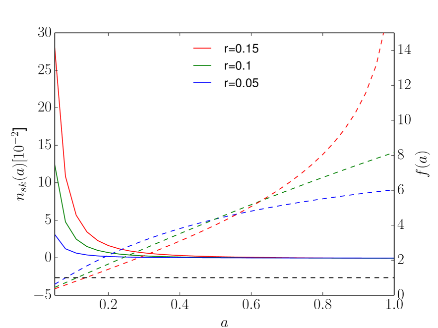
Refer to caption — Figure 1: Plot of $n_{sk}$ (solid lines) and $f$ (dashed lines) as functions of $a$ , at fixed $n_{s}=0.96$ for $r=0.05,0.1,0.15$ values, and as dictated by Eqs. (17) and (19) respectively. Notice that for small $a$ the running becomes large; on the other hand when $a$ approaches unity (black dashed line) the running tends to vanish. In this case results are very similar to just considering the case $n_{sk}=0$ . We analyse specific cases in Sec. 3.

Let us now focus on the inflationary sector of the model given by the potential of Eq. (1). The running and running of the running of the scalar power spectrum satisfy the following relations [22]

	$\displaystyle n_{sk}$	$\displaystyle=$	$\displaystyle\frac{r}{32}\left(3r-16\delta_{ns}+\frac{8}{f^{2}}\right),$		(17)
	$\displaystyle n_{skk}$	$\displaystyle=$	$\displaystyle\frac{r}{128}\left(3r^{2}+\frac{12}{f^{2}}r-32\left(2\delta_{ns}-\frac{1}{f^{2}}\right)\delta_{ns}\right).$		(18)

From Eq. (4) for the spectral index we obtain an expression for $f$ involving the second parameter of the model, $a$ :

f=\frac{4a}{\left(r\left(1-3a^{2}\right)+8a^{2}\delta_{ns}+\sqrt{4a^{2}\left(4\delta_{ns}-r\right)^{2}+r^{2}\left(1-a^{2}\right)}\right)^{1/2}}.

(19)

It is thus evident that in a slow-roll stage, this model is fully described in terms of the parameter $a$ alone. The HNI model allows for more flexibility in the potential, since the constraint coming from the number of e-folds does not fix $f$ . The end of inflation is specified by a waterfall field which plays no role during inflation. When considering the particular case $a=1$ we are reduced to a waterfall version of Natural Inflation.

In Fig. 1, we plot $f$ and $n_{sk}$ in terms of $a$ , at a fixed $n_{s}=0.96$ and for $r=0.05,0.1,0.15$ values. If we assume the values of BICEP2 of the order $r\sim 0.15$ (red lines), for $a=1$ the running tends to be very close to zero and $f>>1$ . On the other hand, if we consider values allowed by Planck (blue lines), $f$ values decreases to order $f\sim 6$ . Similarly for $f=1$ values (black dashed line), $a$ tends to be order of $a\sim 0.1$ and hence $n_{sk}\sim 0.1$ for BICEP2 and $n_{sk}\sim 0.01$ for Planck values (see however subsection 3.3, where we fix $f$ to the value $f=1$ and study its consequences).

From Fig. 1 we can identify the corner of parameter space where a theoretically consistent value for $f$ ( $\leq 1$ ) is obtained during slow-roll. We go further to constrain the HNI model by employing the most recent tracers of the CMB. In particular, we use the latest release of Planck dataset [13] which, combined with the nine-year WMAP polarisation maps [14], allow to constrain the temperature and polarisation spectra (T, E and B components). Furthermore, we provide a joint-analysis with the BICEP2 data release [15], interpreting these results as a non-vanishing tensor contributions. To carry out the exploration of the parameter space, we incorporate the HNI potential into the standard cosmological equations, by performing the minor modifications to the CAMB code [23]. We use the CAMB runs to explore the parameter space with the software CosmoMC [24].

Throughout the analysis we consider purely Gaussian adiabatic scalar and tensor perturbations. We assume a standard $\Lambda$ CDM model specified by the following parameters: the physical baryon density $\Omega_{\rm b}h^{2}$ and CDM density $\Omega_{\rm DM}h^{2}$ , where $h$ is the dimensionless Hubble parameter such that $H_{0}=100h$ kms^-1Mpc^-1; $\theta$ , which is $100\times$ the ratio of the sound horizon to angular diameter distance at last scattering surface, and the optical depth $\tau$ at reionisation.

3 Results: Cosmological constraints

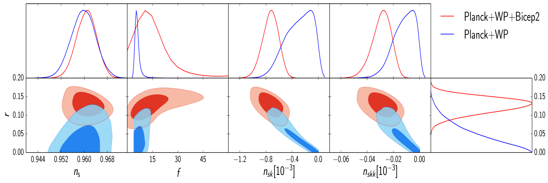
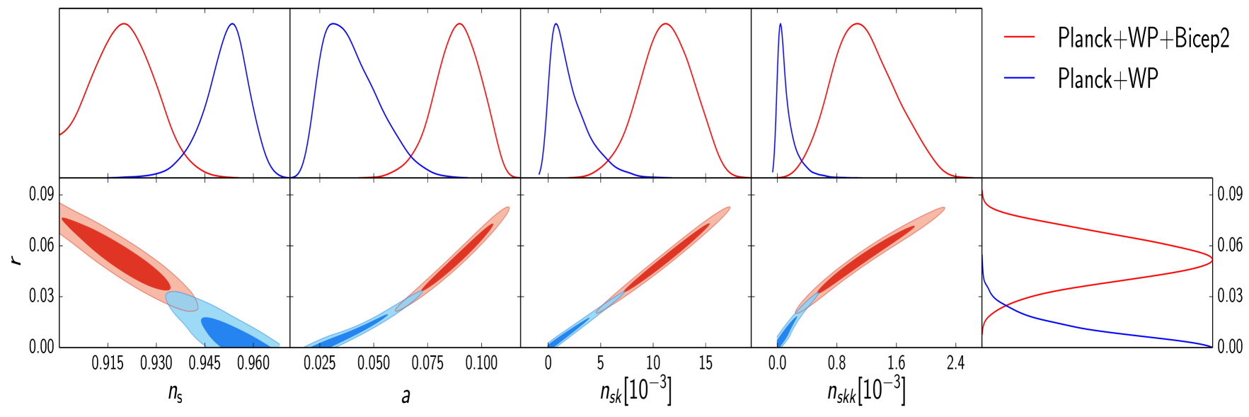
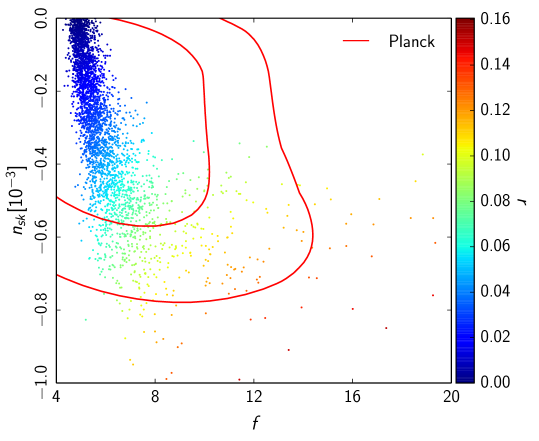
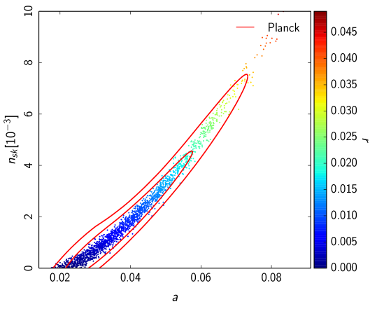
In this section we present the one- and two- $\sigma$ likelihood contours for the set of spectral parameters $\{n_{s},a,f,n_{sk},n_{skk}\}$ ¹¹1We omit plotting the tensor index $n_{t}$ because in the assumed slow-roll regime it is linearly proportional to the tensor-to-scalar ratio $r$ , cf. Eq. (3)., plotted against the tensor to scalar ratio $r$ , in three different cases of the model in Eq. (1). In Sec. 3.1 we study the case when the parameters $\{a,f\}$ are allowed to take any constant value in the range $0<a<1$ and $f>0$ ; In Sec. 3.2 we look at the case of WNI , where we fix $a=1$ a priori; and In Sec. 3.3 the case of $f=1$ is studied. This is justified as a just realistic value for the symmetry breaking parameter $f$ .

3.1 Full Hybrid Natural Inflation

As introduced above, the HNI model features $a$ as a free parameter taking any value in the interval $0<a<1$ . With the scale $f$ allowed to take any given positive value, Fig. 2 shows the likelihood contours which present no degeneracy between parameters. From the figure we can read a small running consistent with $n_{sk}=0$ , both in the analysis using Planck+WP data only and the combined Planck+WP+BICEP2 data. The results suggest that, when leaving $f$ arbitrary, HNI shows no significant improvement over WNI since $f$ has to be bigger that one and the running uninterestingly small. More interestingly, the Planck+WP+BICEP2 data favour a vanishing running but with a parameter $a$ close to one ( $0.8$ ) and $f\approx 8$ as shown in Table 1, instead of the small and always negative running of WNI with $a=1$ and larger $f$ [25]. The preferred value of $a$ approaching unity is close to the standard NI model.

3.2 Hybrid Natural Inflation with $a=1$

The case $a=1$ corresponds to a slight generalization of NI. Released from the requirement to end inflation, aided by a waterfall field, we consider the special case of Waterfall Natural Inflation (WNI) (for a recent study of the consistency of standard NI with CMB observations of Planck and BICEP2 see [25]). The likelihood contours for this case are presented in Fig. 3. A certain degeneracy is observed between $r$ and the running parameter $n_{sk}$ when analysing the Planck+WP data alone. Such degeneracy is broken when BICEP2 observations are added to the dataset. Additionaly, note that the area of overlap of both datasets is marginally smaller than the previous case. Note that the preferred value of the symmetry breaking scale $f$ for WNI still lies above unity.

3.3 Hybrid Natural Inflation with $f=1$

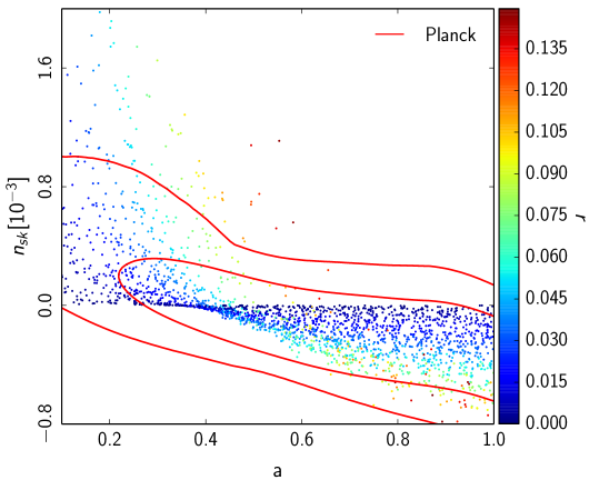
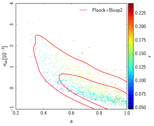
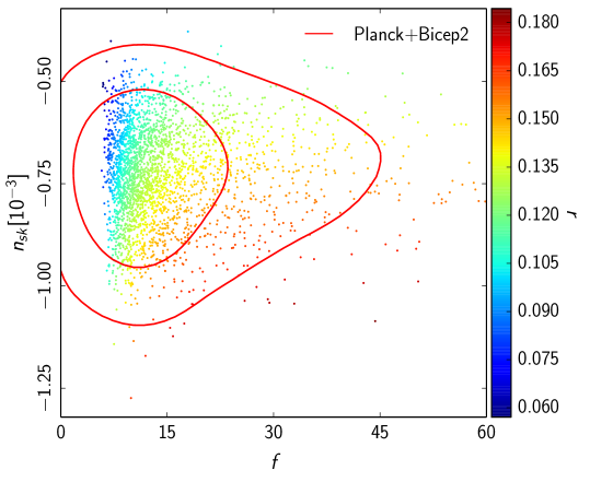
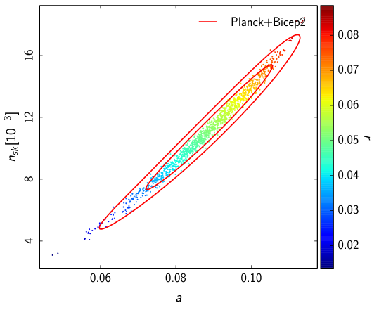
One of the main motivations for introducing the model of HNI [10, 11], where the end of inflation is not triggered by the slow-rolling inflaton field but by a second waterfall field, is to release the parameter $f$ from inflationary constraints and to have values equal or less than the Planck scale. Being $f$ the scale of (Nambu-Goldstone) symmetry breaking it is desirable not to surpass the Planck value as occurs in ordinary NI, where the same field which produces inflation is also in charge of terminating it. What we see from Fig. 4 is that HNI with $f=1$ is consistent with Planck+WP data alone but, when taking running through the BICEP2 dataset the overlap is almost vanishing. This evidences a strong tension between the two datasets for the model. Also, a set value for the parameter $f$ , means that the single degree of freedom $a$ determines the value of the other parameters. This is evident from the plots which reveal a strong correlation between $r$ and the rest of the spectral parameters. We analyse the consequences of these results for the validity of the models in the next section.

HNI	$f$	$a$	$r$	$n_{s}$	$n_{sk}$
Case: general
PL+WP	$4.5$	$0.60$	$<0.09$	$0.96$	$-4\times 10^{-5}$
PL+WP+BP2	$8.0$	$>0.42$	$0.14$	$0.96$	$<1.6\times 10^{-3}$
Case: $a=1$
PL+WP	$6.1$	$1$	$<0.1$	$0.96$	$-3\times 10^{-4}$
PL+WP+BP2	$17.2$	$1$	$0.13$	$0.96$	$-7\times 10^{-4}$
Case: $f=1$
PL+WP	$1$	$0.04$	$<0.02$	$0.95$	$2\times 10^{-3}$
PL+WP+BP2	$1$	$0.09$	$0.05$	$0.92$	$1\times 10^{-2}$

Table 1: We show approximate mean values and bounds for the model parameters

f

and

a

(when not fixed) as well as for the tensor

r

, spectral index

n_{s}

and running

n_{sk}

for three cases of hybrid natural inflation using Planck+WMAP data only (PL+WP) and Planck+WMAP+BICEP2 data (PL+WP+BP2). We confirm that for the case of two free parameters

\{a,f\}

, HNI is no real improvement over a Waterfall Natural Inflation model (i.e. the

a=1

case). The different values for

r

in these two cases essentially correspond respectively to adjustments in

a

and

f

, and

f

alone, which however do not affect the spectral index value. When we fix the scale of symmetry breaking

f

to one (in Planck units), we see that there is a clear distinction between results. HNI is consistent with PL+WP data alone, but then becomes disfavoured when PL+WP+BP2 data is considered.

4 Consistency checks: $f\leq 1$ and bounds on Primordial Black Holes abundance

Let us now analyse the results presented above in terms of the self-consistency of the models and the consistency with the constraints imposed by the null observations of primordial black holes. From Figs. 2 and 3, we immediately read that the model requires a symmetry breaking parameter $f$ with a value well above the Planck scale which we consider undesirable. Requiring that the scale $f$ is at most $f=1$ , in Planck units, we get Fig. 4 where we see that HNI is still compatible with the Planck+WP data. When combined with the BICEP2 data however, we find that there is a strong tension between the two datasets with an almost vanishing overlap. This is most evident from the combined data plotted in Fig. 5. To get a handle of these results we present in Table 1 the mean values for the model parameters $f$ and $a$ as well as for the observable tensor $r$ , spectral index $n_{s}$ and running $n_{sk}$ for the three cases of HNI studied here.

When, for the case $f=1$ , we combine both datasets there is an additional constraint coming from the possible over-production of primordial black holes (PBHs). The large positive value of the running $n_{sk}$ in Fig. 4 (see also Fig. 1), could invert the red spectrum of scalar perturbations and induce, at small scales, inhomogeneities with amplitudes ruled out by observations. Following the argument of [16], the undesired amplitude for perturbations at which PBHs could be over-produced is $\mathcal{P}_{s}(N=0)\simeq 10^{3}$ (see also Refs. [26, 27]). Since this is most likely to happen toward the end of inflation, when the number of remaining e-folds of inflation is $N\approx 0$ , the inflaton field has the order of 50 or 60 e-folds to evolve from the initial $\mathcal{P}_{s}=10^{-9}$ to the PBHs overproduction value. The Taylor expansion of the power spectrum around its observed value at $N_{i}=50\text{ to }60$ shows that ²²2Note that, to lowest order in slow-roll $d/dN=-d/dk$ ,

\ln\left[\frac{\mathcal{P}_{s}(0)}{\mathcal{P}_{s}(N_{i})}\right]=(n_{s}-1)N_{i}+\frac{1}{2}n_{sk}N_{i}^{2}.

(20)

In writing this equation we have ignored derivatives of the power spectrum at orders higher than two. Such truncated expansions may seem incomplete to evaluate the amplitude of the spectrum, at about 50 e-folds away from observable scales, but they have been successfully employed to constrain undetermined parameters (e.g. [28, 16, 17]). Our equation (20) is only a first approximation to establish a bound on the undetermined value of the running $n_{sk}$ and therefore to constrain the predictions of HNI.³³3We have checked that the next order term in the expansion of Eq. (20), involving the parameter $n_{skk}$ , is subdominant with respect to those appearing in the equation.

Upon substitution of values of $\mathcal{P}_{s}(0)$ that over-produce PBHs, we find that the left hand side should not exceed the value of about 14. The right hand side then imposes a constraint on positive values of the running. Substituting the values of Table 1 we see that the HNI model with $f=1$ is restricted to values of the running $n_{sk}<0.0104$ , which practically excludes the central value of the parameter adjusting the Planck+WP+BICEP2 data. Note that for this same model, the Planck+WP data yield a smaller value of $n_{sk}\approx 10^{-3}$ , which is not excluded by the abundance of PBHs. Our calculation shows that, when the BICEP2 data is interpreted as a signature of primordial gravitational waves, the model of HNI with $f=1$ would be discarded.

5 Summary and conclusions

We find that when the scale of symmetry breaking $f$ is left unrestricted, Hybrid Natural Inflation is not essentialy different from natural inflation both favouring a small running consistent with a vanishing value. The case where $f=1$ , however, is consistent with Planck+WP data alone but not when combined with BICEP2 data. This is shown in Fig. 4 evidencing a strong tension between both data sets. Table 1 shows that when the Planck+WP+BICEP2 data is used, HNI with $f=1$ is disfavoured since the spectral index starts moving away from observed values. At the ultraviolet end of the spectrum, the over-production of PBHs imposes a bound on the value of the running $n_{sk}\lesssim 0.01$ . This has also been reported in previous works of single-field inflation: for running mass inflation [16] and for the more general hilltop inflationary models [17]. The common feature shared by these models and HNI is that the slope of the inflationary potential flattens toward the end of inflation, allowing for both a large number of e-folds and an enhancement in the amplitude of field fluctuations.

Two comments are in place regarding the validity of constraints derived from BICEP2 and the bounds to PBHs abundance. Recent observations [29] have raised doubts regarding the cleanliness of the BICEP2 data. Additionally, our results seem to support the argument that BICEP2 data at face value may be incompatible with slow-roll inflation in general [30]. Thus, a conclusive analysis on the feasibility of HNI awaits more data.

On the other hand, recent studies have shown that the formation of PBHs is not solely determined by the amplitude of perturbations. Indeed, not all profiles of overdensities with a common amplitude will get to form PBHs [31, 32], and the probability of formation might be significantly reduced, [33]. On the other hand, the overproduction of PBHs at the end of inflation could trigger the subsequent reheating period [34]. While this argument requires fine-tuning, it is worth exploring the final stages of inflation since, in addition to the analysis above, a waterfall field, like the one expected to end inflation in the models studied here, is likely to produce PBHs copiously at the end of inflation [35]. We leave the study of these possibilities for future work.

In conclusion, our results show that when we force HNI to desirable values of the symmetry breaking parameter, the $f=1$ case is compatible with Planck+WP-only data but not when combined with BICEP2 since a smaller spectral index $n_{s}$ is favoured and over-production of PBHs at the end of inflation occurs. This disagreement is not yet ruling out the $f=1$ scenario given that the polarisation data from Planck [29], indicates that the signal detected by BICEP2 may be completely due to galactic dust. A forthcoming cross-correlation of the data from both experiments will reveal the nature of the BICEP2 observations.

6 Acknowledgements

We gratefully acknowledge support from Programa de Apoyo a Proyectos de Investigación e Innovación Tecnológica (PAPIIT) UNAM, IN103413-3, Teorías de Kaluza-Klein, inflación y perturbaciones gravitacionales and IA101414-1, Fluctuaciones no-lineales en cosmología relativista. AHA is grateful to the staff of ICF, UNAM and UAM-Iztapalapa for hospitality. MCG acknowledges a scholarship from PI and CONACyT. JAV, GG, AHA and JCH thank SNI for support.

References

[1] A.H. Guth, Phys. Rev. D23 (1981) 347.
[2] A.D Linde, Phys. Lett. B108 (1982) 389.
[3] A. Albrecht and P.J. Steinhardt, Phys. Rev. Lett. 48 (1982) 1220.
[4] For reviews see e.g., D. H. Lyth and A. Riotto, Phys. Rept. 314 (1999) 1 [hep-ph/9807278]; D. H. Lyth and A. R. Liddle, Cambridge, UK: Cambridge Univ. Pr. (2009) 497 p; D. Baumann, “TASI Lectures on Inflation,” arXiv:0907.5424 [hep-th].
[5] J. A. Vázquez, A. N. Lasenby, M. Bridges, and M. P. Hobson. MNRAS, 422(3):1948–1956, 2012, [arXiv:1103.4619].
[6] J. A. Vazquez, M. Bridges, M. Hobson, and A. Lasenby. JCAP, 2012 06:06, [arXiv:1203.1252].
[7] K. Freese, J. A. Frieman and A. V. Olinto, Phys. Rev. Lett. 65 (1990) 3233.
[8] F. Adams, J.R. Bond, K. Freese, J. A. Frieman and A. V. Olinto, Phys. Rev.D47 (1993) 426-455.
[9] K. Freese, C. Savage and W. H. Kinney, Int. J. Mod. Phys. D 16 (2008) 2573 [arXiv:0802.0227 [hep-ph]].
[10] G. G. Ross and G. German, Phys. Lett. B 684 (2010) 199 [arXiv:0902.4676 [hep-ph]].
[11] G. G. Ross and G. German, Phys. Lett. B 691 (2010) 117 [arXiv:1002.0029 [hep-ph]].
[12] A. Linde, Phys. Rev. D 49 (1994) 748; Other general references for hybrid inflation are: D.H. Lyth, A. Riotto, Phys. Rep. 314 (1999) 1, arXiv:hep-ph/9807278; A.D. Linde, Lecture Notes in Phys. 738 (2008) 1, arXiv:0705.0164 [hep-th]; M. Shaposhnikov, J. Phys. Conf. Ser. 171 (2009) 012005.
[13] P. A. R. Ade et al. [Planck Collaboration], arXiv:1303.5082 [astro-ph.CO].
[14] C. L. Bennett et al. [WMAP Collaboration], ApJS 208 (2013) 20B arXiv:1212.5225 [astro-ph.CO].
[15] P. A. R. Ade et al. [BICEP2 Collaboration], Phys. Rev. Lett. 112 (2014) 241101 [arXiv:1403.3985 [astro-ph.CO]].
[16] K. Kohri, D. H. Lyth and A. Melchiorri, JCAP 0804 (2008) 038 [arXiv:0711.5006 [hep-ph]].
[17] L. Alabidi and K. Kohri, Phys. Rev. D 80 (2009) 063511 [arXiv:0906.1398 [astro-ph.CO]].
[18] A. R. Liddle, P. Parsons and J. D. Barrow, Phys. Rev. D 50 (1994) 7222 [astro-ph/9408015].
[19] A. R. Liddle and D. H. Lyth, Cosmological Inflation and Large-Scale Structure, Cambridge University Press, (2000).
[20] J. A. Vazquez, M. Bridges, Yin-Zhe Ma, and M. Hobson. JCAP 1308 (2013) 001, [arXiv:1303.4014].
[21] Brian A. Powell, [arXiv:1209.2024].
[22] M. Carrillo-González, G. Germán, A. Herrera-Aguilar, J. C. Hidalgo and R. Sussman, Phys. Lett. B 734 (2014) 345 [arXiv:1404.1122 [astro-ph.CO]].
[23] A. Lewis, A. Challinor and A. Lasenby, Astrophys. J. 538 (2000) 473 [astro-ph/9911177].
[24] A. Lewis and S. Bridle Phys. Rev. D, 66 (2002) 103511 [arXiv:0205436 [astro-ph.CO]].
[25] K. Freese and W. H. Kinney, arXiv:1403.5277 [astro-ph.CO].
[26] A. S. Josan, A. M. Green and K. A. Malik, Phys. Rev. D 79 (2009) 103520 [arXiv:0903.3184 [astro-ph.CO]].
[27] B. J. Carr, K. Kohri, Y. Sendouda and J. Yokoyama, Phys. Rev. D 81 (2010) 104019 [arXiv:0912.5297 [astro-ph.CO]].
[28] B. J. Carr, J. H. Gilbert and J. E. Lidsey, Phys. Rev. D 50 (1994) 4853 [astro-ph/9405027].
[29] R. Adam et al. [Planck Collaboration], arXiv:1409.5738 [astro-ph.CO].
[30] M. Cortês, A. R. Liddle and D. Parkinson, arXiv:1409.6530 [astro-ph.CO].
[31] A. G. Polnarev and I. Musco, Class. Quant. Grav. 24 (2007) 1405 [gr-qc/0605122].
[32] T. Nakama, T. Harada, A. G. Polnarev and J. Yokoyama, JCAP01(2014)037 [arXiv:1310.3007 [gr-qc]].
[33] J. C. Hidalgo and A. G. Polnarev, Phys. Rev. D 79 (2009) 044006 [arXiv:0806.2752 [astro-ph]].
[34] J. C. Hidalgo, L. A. Urena-Lopez and A. R. Liddle, Phys. Rev. D 85 (2012) 044055 [arXiv:1107.5669 [astro-ph.CO]].
[35] D. H. Lyth, JCAP 1205 (2012) 022 [arXiv:1201.4312 [astro-ph.CO]].