Constraints on cosmic rays in the Milky Way circumgalactic medium from OVIII observations
Abstract
We constrain the cosmic ray (CR) population in the circumgalactic medium (CGM) of Milky Way by comparing the observations of absorption lines of OVIII ion with predictions from analytical models of CGM : precipitation (PP) and isothermal (IT) model. For a CGM in hydrostatic equilibrium, the introduction of CR suppresses thermal pressure, and affects the OVIII ion abundance. We explore the allowances given to the ratio of CR pressure to thermal pressure (), with varying boundary conditions, CGM mass content, photoionization by extragalactic ultraviolet background and temperature fluctuations. We find that the allowed maximum values of are : in the PP model and in the IT model. We also explore the spatial variation of : rising () or declining () with radius, where A is the normalization of the profiles. In particular, the models with declining ratio of CR to thermal pressure fare better than those with rising ratio with suitable temperature fluctuation (larger for PP and lower for IT). The declining profiles allow and in the case of IT and PP models, respectively, thereby accommodating a large value of in the central region, but not in the outer regions. These limits, combined with the limits derived from -ray and radio background, can be useful for building models of Milky Way CGM including CR population. However, the larger amount of CR can be packed in cold phase which may be one way to circumvent these constraints.
1 Introduction
Galaxies have two components: galactic disk surrounded by a gaseous and a dark matter halo. The gaseous halo, which extends up to the virial radius (sometimes even beyond) is known as the circumgalactic medium (CGM). It is a reservoir for most of the baryons and plays a crucial role in galaxy formation and evolution by various feedback processes such as outflowing, recycling of gas (Tumlinson et al., 2017). Soft -ray observation of OVII and OVIII absorption (Gupta et al., 2012; Fang et al., 2015) and emission lines (Henley et al., 2010; Henley & Shelton, 2010), and SZ effect (Planck Collaboration et al., 2013; Anderson et al., 2015) indicate the presence of a hot phase (T K) of CGM. Recently, a warm (K) and a cool phase (K) of CGM have also been discovered through absorption lines of low and intermediate ions 111Low Ions: Ionization Potential (IP) eV, T K; Intermediate Ions: IP (eV) , T K; High Ions: IP, TK. (Tumlinson et al., 2017) at low redshifts (Stocke et al., 2013; Werk et al., 2014, 2016; Prochaska et al., 2017a) and Ly emission at high redshifts (Hennawi et al., 2015; Cai et al., 2017). It is not yet clear how this cool phase coexists with the hot phase and survives the destructive effects of various instabilities (McCourt et al., 2015; Ji et al., 2018), but this discovery has led to a picture of multiphase temperature and density structure of the CGM (Tumlinson et al., 2017; Zhang, 2018). It also partially solves the problem of missing baryon in the galaxies (Tumlinson et al., 2017).
If the CGM is considered to be in hydrostatic equilibrium by means of only thermal pressure, then in order to maintain pressure equilibrium the cold component ( K) of CGM is expected to have a higher density than the hot component ( K). However, Werk et al. (2014) found the density of cold gas to follow the hot gas density distribution. This has given rise to the idea of a non-thermal pressure component, consisting of cosmic-ray (CR) and magnetic pressure which can add to the thermal pressure. Without a non-thermal component, the abundances of low and mid-ions (seen in cool and warm phases, respectively) are under-estimated even in high-resolution simulations (van de Voort et al., 2019; Hummels et al., 2019; Peeples et al., 2019). Ji et al. (2020) have suggested that CR can explain these two problems. It has been suggested that CR can provide pressure support to cool diffuse gas (Salem et al., 2015; Butsky & Quinn, 2018), help in driving galactic outflows (Ruszkowski et al., 2017; Wiener et al., 2017), as well as excite Alfvén waves that can heat the CGM gas (Wiener et al., 2013).
The magnitude of the CR population in the CGM is, however, highly debated. Some simulations (Butsky & Quinn, 2018; Ji et al., 2020; Dashyan & Dubois, 2020) claimed a CR dominated halo, which increases feedback efficiency of the outflowing gas by increasing the mass loading factor and suppressing the star formation rate. The ratio of CR pressure and thermal pressure () controls this effect and can reach a large value exceeding 10 over a huge portion of Milky-way sized halo (Butsky & Quinn, 2018). Another simulation claimed that MW-sized halo at low redshift (z) can be CR populated with nearly in outflow regions, although in warm regions (T= K) of halo, (Ji et al., 2020). Dashyan & Dubois (2020) found in their simulation that dwarf galaxies, with virial mass M⊙, can have a high value of () at kpc from the mid-plane when isotropic diffusion is incorporated (their figure 1 and 2 ).
It is therefore an important question as to how much CR can be accommodated in the CGM in light of different observations. One of the most obvious effects of CR population in CGM is to suppress the thermal pressure of the hot phase which is also seen in the simulation of Ji et al. (2020). The recent work by Kim et al. (2021) pointed out that this reduction in thermal pressure would lower the thermal SZ (tSZ) signal, as tSZ probes the integrated thermal pressure in the halo. This diminished value of thermal pressure would also significantly change the abundance of high ionization species, and thereby jeopardise the interpretation of their column densities. In a recent work by Faerman et al. (2021), they modified their previous isentropic model Faerman et al. (2019) with significant non-thermal pressure () and found that the gas temperature in the central region for the non-thermal model becomes lower than the value at which OVIII CIE temperature peaks, which in turn results in a lower OVIII column density. At low CGM masses, photoionization compensated for this effect by the formation of OVIII at larger radii, but for large gas masses and large mean densities (as in the Milky Way), photoionization effect is negligible and the total OVIII column density is low. In a previous work (Jana et al., 2020), we constrained the CR pressure () in the CGM in light of the isotropic -ray background (IGRB) and radio background, using different analytical models (Isothermal Model: IT, Precipitation Model: PP) of CGM. In the case of IT model, the value of IGRB flux puts an upper limit of 3 on , whereas all values of are ruled out if one considers the anisotropy of the flux due to off-center position of solar system in Milky Way. However, in the case of PP model, IGRB flux value and its anisotropy allow a range of from 100 to 230. In comparison, the constraints from radio background are not quite robust. In this paper, we use the same analytical models (IT and PP) and put limits on CR population in the CGM of Milky Way by comparing the predicted OVIII absorption column densities (NOVIII) with the available observations.
It might still be asked, why use OVIII as a probe? Previous works (Faerman et al., 2017; Roy et al., 2021) explained the observed OVII, OVIII absorption column densities in the Milky Way without the incorporation of CR component using the analytical models of CGM used here. It is, therefore, important to study the effect of CR on these column densities with the inclusion of CR component in these models. Whereas the OVII ion has a plateau of favourable temperatures ( K - K), the suitable temperature for OVIII production (K) peaks near the temperature of the hot halo gas of Milky Way CGM. This particular fact makes OVIII abundance a sensitive probe of the CGM hot gas and motivates the choice of OVIII column density for comparison with the observations in order to constrain CR population in Milky Way CGM.
2 Density and Temperature Models
We study two widely discussed analytical models: 1) Isothermal Model (IT), 2) Precipitation Model (PP). These models have previously been studied in the context of absorption and emission lines from different ions (Faerman et al., 2017; Voit, 2019; Roy et al., 2021) We assume the CGM to be in hydrostatic equilibrium within the potential of dark matter halo () , with a metallicity of Z⊙ (Prochaska et al., 2017b), so that,
| (1) |
where is the total pressure and and r are the density and radius, respectively. We consider the Navarro-Frenk-White (NFW) (Navarro et al., 1996) profile as the underlying dark matter potential in the IT model. However we slightly modify this potential in the case of the PP model as suggested in Voit (2019) by considering the circular velocity (vc) to be constant (v km s-1) up to a radius of for a halo with M M⊙ and concentration parameter . We include non-thermal pressure support with CR population and magnetic field along with thermal pressure in these models. We consider the magnetic energy to be in equipartition with thermal energy (Pmag=Pth) so that the total pressure , which leads to,
| (2) |
Note that the magnitude of magnetic field in CGM is rather uncertain. While Bernet et al. (2008) claimed the magnetic field in CGM of galaxies at to be larger than that in present day galaxies, the observations of Prochaska et al. (2019) suggested a value less than that given by equipartition. Yet another study claimed near-equipartition value after correlating the rotation measures of high- radio sources with those in CGM of foreground galaxies (Lan & Prochaska, 2020).
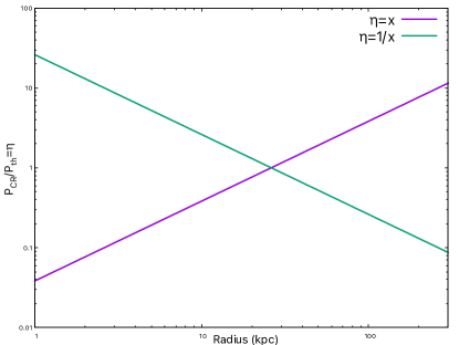
The inclusion of non-thermal pressure suppresses the thermal pressure, and in turn the temperature or density or both of the CGM gas (also seen in recent simulation of Ji et al. (2020)). Our goal is to determine the effect of the inclusion of CR population on NOVIII therefore constrain the CR population in Milky Way CGM. In addition to models with uniform , we have studied the effect of varying as a function of radius. For this, we have explored two contrasting variations, (rising profile) and (declining profile) where x=r/rs, where A is normalization of the profiles. We primarily studied the case with A=1, where the maximum value (for ) is r=c=10. For , to avoid divergence at r=0 kpc we have started our calculation from r=1 kpc, therefore the maximum value in this case is r kpc. We have shown the profiles of in the figure 1. We have explored the effects of scaling up and down the values with these profiles as well (e.g., , with ). Although can vary in a more complicated manner, we study these two particular cases (increasing and decreasing linearly) as the simplest representatives of a class of models in which is allowed to vary with radius. It should be noted that the here denotes the CR pressure in the diffuse hot gas with respect to thermal pressure of the hot gas.
There are several ways to proceed, starting from equation 2. One way is to simply consider the temperature all over the CGM to be constant, which implies the LHS of the equation 2 to be zero. Another way is to use specific entropy to relate the two unknown quantities in the equation 2, temperature and density. We discuss these two ways in details in the following subsections.
2.1 Isothermal Model
The IT model provides the simplest model for the CGM gas with a constant temperature, so that,
| (3) |
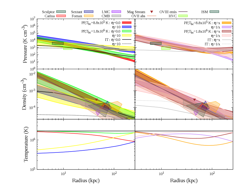
Previously hot gas has been modelled using isothermal profile by Miller & Bregman (2015) where they fitted their model with the OVIII emission line observations which determined the hot gas mass to be within the range of . Therefore, we normalize the density profile isothermal model without any non-thermal component such that the hot gas mass is . It should be noted that the single temperature IT model does not represent the multiphase nature of the CGM. However, OVIII abundance is sensitive mostly to the hot phase of CGM which is well described by the single phase model. Therefore, our limits from the IT model will not change even if we have a two or three temperature model. Another way of incorporating multi-phase in IT model is to consider temperature distribution around the single mean temperature. We will show below that incorporation of such distribution in IT model will tighten our limit on CR. We can, therefore, treat the limit from our single temperature IT model as an upper limit. We then include a non-thermal pressure component in our model along with the thermal pressure. At this point, there are again several ways to proceed. One can fix the mass, and hence the density profile of the hot gas, and compensate for the decrease in thermal pressure by reducing the temperature (Jana et al., 2020). Another way is to fix the temperature and reduce the density by keeping the boundary value same. However, for massive galaxies (M M⊙) (Li et al., 2015) as well as Milky Way (Miller & Bregman, 2015), the halo temperature is observed to be K. This motivates us to assume a constant CGM temperature of K for all the IT model (without and with non-thermal pressure) (Miller & Bregman, 2015). We therefore vary the density profile for different values of by keeping the density at the outer boundary fixed. This lowers the inner density for increasing value of , and for , the hot gas mass becomes - the lower limit of hot gas mass obtained by Miller & Bregman (2015). We, therefore, do not consider larger values of for IT model. In the left panel of Figure 2, density profiles for IT model are shown by black solid () and dotted lines (). The grey solid and dotted lines in the right panel of Figure 2 denote the x and 1/x cases respectively.
2.2 Precipitation Model
The PP model is a physically motivated CGM model which uses the specific entropy as a connection between density and temperature. It is built upon the concept of a threshold limit for the ratio of radiative cooling time (tcool) to free fall time (tff). Recent phenomenological studies and numerical simulations (e.g., McCourt et al., 2012; Sharma et al., 2012; Voit & Donahue, 2015) showed that thermally unstable perturbations can lead to multiphase condensation below this threshold value. In this model, we consider a composite entropy profile () with the combination of base entropy and precipitation-limited entropy.
| (4) |
where base profile is,
| (5) |
and precipitation-limited profile is,
| (6) |
Then using , it follows from equation 2 that,
| (7) |
A recent study by Butsky et al. (2020) has shown the effect of cosmic ray pressure on thermal instability and precipitation for different values of the ratio tcool/tff. In their study, they found that large cosmic ray pressure decreases the density contrast of cool clouds. In our model, we keep tcool/tff to be constant throughout the halo. Although observations and simulations of intercluster medium point towards a value of this ratio between , it is a rather uncertain parameter in case of CGM studies and can have a wide range. We explore a range of the temperature boundary condition (Tbc) at the virial radius, between K (virial temperature of the Milky-way) to K (used originally by Voit (2019)). The inclusion of non-thermal pressure in the model suppresses the temperature and in turn the density. However we keep the mass of the CGM gas constant by decreasing tcool/tff ratio. The variation of tcool/tff with for different values of temperature boundary condition can be seen in Figure 2 of Jana et al. (2020). We have taken the mass of the CGM in a range of M⊙ (from the original model of Voit (2019) without CR) to M⊙ (for cosmic baryon fraction) in case of . However the mass range for is M⊙ since beyond this upper limit of mass, the value of tcool/tff falls below . We use the cooling function from CLOUDY (Ferland et al., 2017) for a metallicity of 0.3Z⊙.
We show the temperature and density profiles for PP in Figure 2 as shaded regions, bracketing the range of CGM mass mentioned above. In the left panel of Figure 2, the temperature and density profiles are shown in green and red for the PP model with no CR component whereas yellow and blue denotes for and respectively. In the right panel of Figure 2, the temperature and density profiles are shown in brown and orange for the PP model with x whereas pink and purple denote 1/x for and respectively.
2.3 Observational constraints
Figure 2 also shows observational limits on pressure, density from (a) observations of OVII and OVIII (Miller & Bregman, 2015), (b) CMB/X-ray stacking (Singh et al., 2018), (c) ram pressure stripping of LMC (Salem et al., 2015), Carina, Sextans (Gatto et al., 2013), Fornax, Sculptor (Grcevich & Putman, 2009), (d) high-velocity clouds (Putman et al., 2012), (e) Magellanic stream (Stanimirović et al., 2002) and (f) ISM pressure (Jenkins & Tripp, 2011). We find that the obtained profiles including non-thermal components are within the observational limits. We can also compare the temperature and density profiles with those from simulations that include CR. In the PP model, the distinguishing feature is a rising temperature profile from the inner to the outer region. CR simulations also show such profiles, e.g., as shown in Figure 5 of Ji et al. (2020), especially beyond the galacto-centric radius of kpc. This particular profile from Ji et al. (2020) shows a decrease in temperature by a factor from the virial radius to kpc, similar to that shown in Figure 2 for cases, although the outer boundary temperature is different in two cases. The difference in the profiles inward of kpc is not significant because the difference caused in the column density is small. The curves on the RHS of Figure 2 for declining cases are similar to the simulation results expect at the outer radii, where PP models predict a declining temperature profile, which is not seen in CR-inclusive simulations. In brief, PP models with with constant or declining profiles appear to capture the CR-simulation temperature (and consequently) density profiles.
2.4 Log-normal Temperature Fluctuation
The observed widths and centroid offsets of OVI absorption lines in the CGM motivate us to consider dynamical disturbances causing temperature fluctuations in the CGM which results in a multiphase CGM gas. Low entropy gas parcels uplifted by outflows or high entropy gas can cool down adiabatically to maintain pressure balance and give rise to temperature and density fluctuations. Turbulence-driven nonlinear oscillations of gravity waves in a gravitationally stratified medium can be an alternative source for these fluctuations. Therefore, we consider an inhomogeneous CGM by including a log-normal temperature distribution (characterized by ) around the mean temperature.
Previous studies have considered a log-normal temperature fluctuation for CGM and successfully matched with CGM observations. Faerman et al. (2017) considered log-normal distribution for their two-temperature (K and K) CGM model. They found the best fit value of to be 0.3 in order to explain the observed OVI column density. We have taken a similar approach. However we have a single temperature IT model. Therefore we consider a log-normal distribution of temperature around the single halo temperature in the case of IT model. In case of PP model, instead of a single temperature, we have a temperature profile . Voit (2019); Roy et al. (2021) took into account temperature fluctuation in PP model by considering log-normal distributions with constant value of around the mean temperature at each radius. Voit (2019) found that satisfies the observed OVI column, whereas Roy et al. (2021) concluded a range of in order to explain the observed OVII, OVIII and their ratio. In the PP model, we follow the similar approach as in Voit (2019); Roy et al. (2021).
3 Results
| Model | CI (without fluctuations) | CI (with fluctuations) | PI | ||||
| G12 | F15 | G12 | F15 | G12 | F15 | ||
| PP | Tbc1 | 0.5 | 6 | – | 10 | 0.5 | 8 |
| Tbc2 | – | 0.5 | – | 6 | – | 1 | |
| IT | – | 5 | – | 1 | – | 6 | |
We calculate the ionization fraction of OVIII using CLOUDY (Ferland et al., 2017) with the input of density and temperature profiles derived from the CGM models. In order to incorporate temperature fluctuation, we calculate the ionization fraction for all the temperatures in a log-normal distribution using CLOUDY and integrate them over the corresponding log-normal distribution to get a mean ionization fraction. That means, for IT model we get a single mean ionization fraction corresponding to the log-normal distribution around the single temperature of the halo. But for PP model, we will get mean ionization fractions at each radius corresponding to the log-normal distributions with constant value of around the mean temperature at each radius. We consider two cases: collisional ionization and photoionization along with collisional ionization. We use the extragalactic UV background (Haardt & Madau, 2012) at redshift for photoionization. We take into account our vantage point of observation i.e the solar position and calculate the variation of column density with the Galactic latitude and longitude. We consider the median of the column densities for each value of in order to compare with the observations.
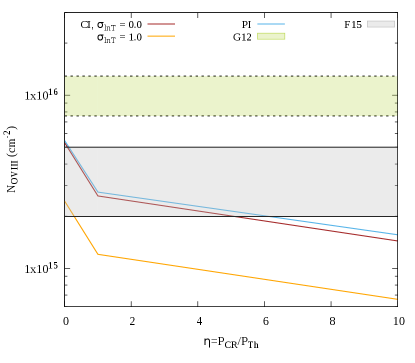
In Figures 3 (for IT model) and 4 (for PP model), we show the variation of NOVIII with , considering collisional ionization (CI) and photoionization (PI) for different models. One can clearly see from these figures that with an increase in , the value of NOVIII decreases due to the decrease in the temperature. In Figure 3, the brown and blue lines denote the cases with CI and PI respectively in the IT model. In this figure, the orange colours denote the effect of log-normal fluctuations (). The cases of CI and PI do not differ for , since at K, CI dominates over PI. However, for , PI leads to slightly larger values of OVIII column density than the CI case, as further decrease in temperature leads to more production of OVIII by PI. It should be noted that if one considers temperature fluctuation around a single favourable temperature of OVIII, there is less OVIII production with the increase in .
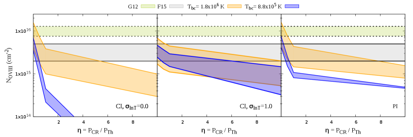
In Figure 4 the orange shaded region indicates the boundary temperature near to virial temperature of halo K (Tbc1) in PP model, whereas the blue shaded region denotes the boundary condition of K (Tbc2) at virial radius. For the PP model, we show the cases with CI without () and with fluctuation () and PI in left, middle and right panel of Figure 4. The shaded regions in this figure refer to the CGM mass range mentioned earlier in the case of PP model. A boundary temperature that is close to the favourable temperature for OVIII yields more OVIII than one gets with lower boundary temperatures. However, with the inclusion of temperature fluctuations, one gets almost similar OVIII for both cases. With lower boundary temperature, the production of OVIII decreases for , because the inclusion of shifts the temperatures from the CI peak of OVIII. However, considering PI in this case can increase the amount of OVIII.
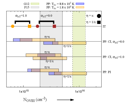
In Figure 5, we show NOVIII with different profiles for both of the models. For IT model, we use brown and orange colours to denote and respectively whereas circles denote x and squares denote 1/x. For PP model, different temperature boundary conditions are shown by orange (T K) and red (T K) shaded regions where shaded region (above the lines for =x and below the lines for =1/x) denote the mass range for each case in PP model. One important point to notice here is that declining profiles produce more OVIII than rising profiles.
3.1 Observations To Compare With
There are some soft X-ray observations of NOVIII of Milky Way by Gupta et al. (2012), Miller & Bregman (2013) and Fang et al. (2015) (Hereafter referred as G12, MB13 and F15 respectively). G12 have measured NOVIII along eight sight lines with Chandra telescope. They have quoted the equivalent width (EW) of OVIII instead of NOVIII in their paper. However, their measured values of EW of OVIII are increased by % for the correction of systematic error and column densities were therefore re-calculated by Faerman et al. (2017). The re-calculated values of log(NOVIII) are respectively. The green shaded region in Figures 3, 4 and 5 show the ranges of of G12 as re-calculated by Faerman et al. (2017).
OVII lines have been studied by MB13 with XMM-Newton along the 26 sight-lines of distant AGNs as well as only one detection of OVIII with ratio of NOVII/NOVIII=. F15 observed the OVII absorption line for a broader sample of 43 AGNs which includes the sample from MB13. They reported a wider range of NOVII ( cm-2) with the central value at cm-2. However they have arrived at these values by setting aside the non-detection along 10 sight-lines. Adding these upper limits to the detected sample, Faerman et al. (2017) have come up with a new range of value of log(NOVII) . Although F15 did not report OVII lines, Faerman et al. (2017) calculated the median of ratio of NOVII and NOVIII from G12 observations. Using this ratio and re-calculated value of NOVII from F15, they calculate log(NOVIII) which ranges from to with a median value of . The grey shaded regions in Figures 3, 4 and 5 show the ranges of NOVII and NOVIII of F15 as re-calculated by Faerman et al. (2017). Note that these re-derived ranges of NOVIII indicate - uncertainty around the median value.
3.2 Constraints
We have tabulated the constraints on for different models in Table 1. It is evident from Figures 3, 4 and 5 NOVIII can help in putting upper limits on . For IT model, we find that if one consider only CI with no temperature fluctuations. The inclusion of PI slightly changes this constraint to . We can also clearly see that introducing log-normal fluctuations makes these constraints even stronger () (Figure 3). Interestingly, we find that the models with varying with radius can be accommodated within observational limits by suitably decreasing (Figure 5). For example, in the Figure 5, the model of increasing with radius for is fairly close to the bottom range of F15’s data, and for the opposite case (), decreasing sufficiently can put in the ballpark of F15’s data.
A larger upper-limit () is allowed for the case of PP model with Tbc1 if one considers of observations of F15. In general, we find that the inclusion of temperature fluctuation relaxes these limits in all the cases by allowing larger value of () (Figure 4). Furthermore, spatial variation of (Figure 5) can be allowed within the observational limits by increasing temperature fluctuations and using suitable mass range in PP model. In particular, models with declining ratio of CR to thermal pressure with radius (as hinted in the simulations of, e.g., Butsky & Quinn (2018)) predict OVIII column densities within observational limits. Note that, in the PP case the requirement for for varying models runs opposite to that in IT, where varying models require smaller in order to be viable.
To see the effect of normalization for the cases or , we have increased the value of , which increases the CR pressure. This leads to a decrease in the density or temperature or both, and consequently decreases the OVIII column density. Therefore, all the plots in Figure 5 will shift towards left with the increment of the normalization. That implies that cases are not allowed for both IT and PP models even with the inclusion of photoionization and temperature fluctuations. However, in the case of the PP model, for with A, all the cases do not satisfy the observational constraints except for the case with boundary temperature K, for . On the other hand, in the case of IT, for the profiles, the OVIII column densities are within the observational constraints for the cases . That implies these models allow the central region to have large CR pressure even , but not in the outer halo. This result differs from the findings by previous simulations which shows CR dominated outer halo (Butsky & Quinn, 2018). As normalization increment shifts all the plots towards left, the inclusion of temperature fluctuations are ruled out for the models with profiles except for a very small range with high CGM mass in the PP model with boundary temperature K and .
4 Discussion
Our constraints allow larger values of for most of the cases in comparison to the isentropic model by Faerman et al. (2019, 2021). In their recent work (Faerman et al., 2021), they have considered three cases for their model : 1) with only thermal pressure i.e, , 2) with standard case as considered in Faerman et al. (2019) i.e, and 3) with significant non-thermal pressure where . Note that the the above mentioned values of are the values at the outer boundary and the profiles of will follow a declining pattern as radius decreases (see blue curve in the right panel of Figure 2 by Faerman et al. (2019)). With our definition of , along with the magnetic field value used by us, we can convert these values to , respectively, for their three cases. The thermal case matches NOVIII observations up to CGM mass of , and for the standard case, the value of NOVIII is comparable to the observed value. However, for the significant non-thermal case, the OVIII value is lower than the observations by a factor of for a CGM mass of . Therefore, one can say that is allowed for the isentropic model. For PP model, we get upper limit of for two cases which are therefore in agreement with the constraint from the isentropic model. However, for most of our models, the upper limits derived in the present work are larger than the isentropic model.
It should be noted that the limits of derived here translate to constraints on cosmic ray pressure in the hot diffuse CGM, and one may wonder about the CR pressure in the cold gas. CR pressure scales with density (, where is the effective adiabatic index of the CR) of the gas, where the adiabatic index depends on the transport mechanism (Butsky et al., 2020), the limits of CR pressure in the cold gas would be different from what we have found for the hot gas. If CRs are strongly coupled to the gas, then in the limit of slow CR transport, i.e, if the only CR transport mechanism is advection, . In this case, CR pressure can be higher in cooler, denser gas than in the hot gas. However, in the limit of efficient CR transport i.e, if there are CR diffusion, streaming along with advection, the CR pressure will be redistributed from high density, cold region to diffuse, hot region of CGM which will lower the . In this limit, , and the limits of CR pressure in the cold phase are nearly equal to the CR pressure in hot phase. In the context of a single phase temperature with temperature gradient, if one considers CR pressure in the hot phase to scale as then is proportional to , as adiabatic index for gas is . Then will be proportional to and respectively depending on slow and effective transport mechanism. This implies that is smaller in denser gas and hence mimic a rising profile of in case of the single hot phase gas, which we have shown in the present paper.
However, these scaling relations are for adiabatic situations, which is not the case for PP model which involves energy loss. In the context of cold gas that may have condensed out of the hot gas, it is possible for the cold gas to contain a significant amount of CR pressure, with a large value of for cold gas. Simulations by Butsky et al. (2020) (their figure 10) showed that in the limit of slow cosmic ray transport, the value of is quite different for hot and cold gas. In the limit of efficient transport, cosmic ray pressure is decoupled from the gas, and has similar values in hot and cold gas. If we recall the observation by Werk et al. (2014), that the cold phase of CGM nearly follows the hot gas density profile then for small density contrast, the CR pressure in the cold phase and hot phase may not differ much even with different transport mechanisms. But even with small density contrast, thermal pressure of cold gas will be smaller than hot phase by two order of magnitude due to the temperature difference, which allows for a larger upper limit on . However, packing more CR in cold gas will not have any effect on the constraints derived here. In fact, this may be one way to circumvent the constraints on described here.
We have not included any disc component in the present work. A recent work by Kaaret et al. (2020) took into account an empirical disc density profile motivated by the measured molecular profile of MW along with the halo component. They pointed out that the high density disc model can well fit the MW’s soft X-ray emission, whereas it under predicts the absorption columns. Their conclusion is that the dominant contribution of X-ray absorption comes from the halo component due to large path length. Also this difference in contribution comes from the fact that the absorption is proportional to density whereas emission measure is proportional to density square. Therefore, considering only the halo component and making the comparison with the absorption column is justified.
Note that the limits derived here are sensitive to some of the parameters such as the magnetic field and metallicity. Increase (decrease) in the magnetic pressure would increase (decrease) the total non-thermal pressure, which would decrease (increase) the limit on . However, given the uncertainty in the magnetic field strength in the CGM, equipartition of magnetic energy with thermal energy is a reasonable assumption. For a collisionally ionized plasma, which we assume for the CGM gas, the column density is proportional to the metallicity () in the case of IT model, whereas it is proportional to for the PP model (see eq 17 of Voit (2019)). In the photoionized case, the dependence on metallicity will be stronger since the ion abundance would also depend on the metallicity. Also note that the limits derived here refer to CR population spread extensively in the CGM. Localized but significant CR population may elude the above limits. However, we also note that most of the contribution of the limits come from the inner region, where OVIII exists otherwise and is suppressed due to CR. Therefore, our limits also pertain to localized CR populations in the inner regions.
5 Summary
We have studied two analytical models of CGM (Isothermal and Precipitation model) in hydrostatic equillibrium in light of the observations of NOVIII in order to constrain the CR population in the Milky Way CGM. We found that in the case of no photoionization and including temperature fluctuations in the PP model whereas IT model allows with inclusion of PI. However, it should be noted that IT is an extremely simplistic model and the inclusion of non-thermal component leads to a very low density. The limits from IT may therefore be only of academic interest.
Combined with the limits derived from -ray background Jana et al. (2020), our results make it difficult for a significant CR population in our Milky Way Galaxy. However, models in which the ratio of CR to thermal pressure varies with radius (preferably declining with radius) can be accommodated within observational constraints, if they include suitable temperature fluctuation (larger for PP and lower for IT), although making allowances for large value of only in the central region.
References
- Anderson et al. (2015) Anderson, M. E., Churazov, E., & Bregman, J. N. 2015, Monthly Notices of the Royal Astronomical Society, 452, 3905, doi: 10.1093/mnras/stv1559
- Bernet et al. (2008) Bernet, M. L., Miniati, F., Lilly, S. J., Kronberg, P. P., & Dessauges-Zavadsky, M. 2008, Nature, 454, 302, doi: 10.1038/nature07105
- Butsky et al. (2020) Butsky, I. S., Fielding, D. B., Hayward, C. C., et al. 2020, ApJ, 903, 77, doi: 10.3847/1538-4357/abbad2
- Butsky & Quinn (2018) Butsky, I. S., & Quinn, T. R. 2018, ApJ, 868, 108, doi: 10.3847/1538-4357/aaeac2
- Cai et al. (2017) Cai, Z., Fan, X., Bian, F., et al. 2017, ApJ, 839, 131, doi: 10.3847/1538-4357/aa6a1a
- Dashyan & Dubois (2020) Dashyan, G., & Dubois, Y. 2020, arXiv e-prints, arXiv:2003.09900. https://arxiv.org/abs/2003.09900
- Faerman et al. (2021) Faerman, Y., Pandya, V., Somerville, R. S., & Sternberg, A. 2021, arXiv e-prints, arXiv:2107.02182. https://arxiv.org/abs/2107.02182
- Faerman et al. (2017) Faerman, Y., Sternberg, A., & McKee, C. F. 2017, ApJ, 835, 52, doi: 10.3847/1538-4357/835/1/52
- Faerman et al. (2019) Faerman, Y., Sternberg, A., & McKee, C. F. 2019, Massive Warm/Hot Galaxy Coronae: II – Isentropic Model. https://arxiv.org/abs/1909.09169
- Fang et al. (2015) Fang, T., Buote, D., Bullock, J., & Ma, R. 2015, ApJS, 217, 21, doi: 10.1088/0067-0049/217/2/21
- Ferland et al. (2017) Ferland, G. J., Chatzikos, M., Guzmán, F., et al. 2017, The 2017 Release of Cloudy. https://arxiv.org/abs/1705.10877
- Gatto et al. (2013) Gatto, A., Fraternali, F., Read, J. I., et al. 2013, MNRAS, 433, 2749, doi: 10.1093/mnras/stt896
- Grcevich & Putman (2009) Grcevich, J., & Putman, M. E. 2009, ApJ, 696, 385, doi: 10.1088/0004-637X/696/1/385
- Gupta et al. (2012) Gupta, A., Mathur, S., Krongold, Y., Nicastro, F., & Galeazzi, M. 2012, ApJ, 756, L8, doi: 10.1088/2041-8205/756/1/L8
- Haardt & Madau (2012) Haardt, F., & Madau, P. 2012, ApJ, 746, 125, doi: 10.1088/0004-637X/746/2/125
- Henley & Shelton (2010) Henley, D. B., & Shelton, R. L. 2010, ApJS, 187, 388, doi: 10.1088/0067-0049/187/2/388
- Henley et al. (2010) Henley, D. B., Shelton, R. L., Kwak, K., Joung, M. R., & Mac Low, M.-M. 2010, ApJ, 723, 935, doi: 10.1088/0004-637X/723/1/935
- Hennawi et al. (2015) Hennawi, J. F., Prochaska, J. X., Cantalupo, S., & Arrigoni-Battaia, F. 2015, Science, 348, 779, doi: 10.1126/science.aaa5397
- Hummels et al. (2019) Hummels, C. B., Smith, B. D., Hopkins, P. F., et al. 2019, ApJ, 882, 156, doi: 10.3847/1538-4357/ab378f
- Jana et al. (2020) Jana, R., Roy, M., & Nath, B. B. 2020, ApJ, 903, L9, doi: 10.3847/2041-8213/abbee4
- Jenkins & Tripp (2011) Jenkins, E. B., & Tripp, T. M. 2011, The Astrophysical Journal, 734, 65, doi: 10.1088/0004-637x/734/1/65
- Ji et al. (2018) Ji, S., Oh, S. P., & McCourt, M. 2018, Monthly Notices of the Royal Astronomical Society, 476, 852, doi: 10.1093/mnras/sty293
- Ji et al. (2020) Ji, S., Chan, T. K., Hummels, C. B., et al. 2020, MNRAS, 496, 4221, doi: 10.1093/mnras/staa1849
- Kaaret et al. (2020) Kaaret, P., Koutroumpa, D., Kuntz, K. D., et al. 2020, Nature Astronomy, 4, 1072, doi: 10.1038/s41550-020-01215-w
- Kim et al. (2021) Kim, J., Golwala, S., Bartlett, J. G., et al. 2021, arXiv e-prints, arXiv:2110.15381. https://arxiv.org/abs/2110.15381
- Lan & Prochaska (2020) Lan, T.-W., & Prochaska, J. X. 2020, MNRAS, 496, 3142, doi: 10.1093/mnras/staa1750
- Li et al. (2015) Li, Y., Bryan, G. L., Ruszkowski, M., et al. 2015, ApJ, 811, 73, doi: 10.1088/0004-637X/811/2/73
- McCourt et al. (2015) McCourt, M., O’Leary, R. M., Madigan, A.-M., & Quataert, E. 2015, MNRAS, 449, 2, doi: 10.1093/mnras/stv355
- McCourt et al. (2012) McCourt, M., Sharma, P., Quataert, E., & Parrish, I. J. 2012, MNRAS, 419, 3319, doi: 10.1111/j.1365-2966.2011.19972.x
- Miller & Bregman (2013) Miller, M. J., & Bregman, J. N. 2013, ApJ, 770, 118, doi: 10.1088/0004-637X/770/2/118
- Miller & Bregman (2015) —. 2015, ApJ, 800, 14, doi: 10.1088/0004-637X/800/1/14
- Navarro et al. (1996) Navarro, J. F., Frenk, C. S., & White, S. D. M. 1996, ApJ, 462, 563, doi: 10.1086/177173
- Peeples et al. (2019) Peeples, M. S., Corlies, L., Tumlinson, J., et al. 2019, ApJ, 873, 129, doi: 10.3847/1538-4357/ab0654
- Planck Collaboration et al. (2013) Planck Collaboration, Ade, P. A. R., Aghanim, N., et al. 2013, A&A, 557, A52, doi: 10.1051/0004-6361/201220941
- Prochaska et al. (2017a) Prochaska, J. X., Werk, J. K., Worseck, G., et al. 2017a, ApJ, 837, 169, doi: 10.3847/1538-4357/aa6007
- Prochaska et al. (2017b) —. 2017b, ApJ, 837, 169, doi: 10.3847/1538-4357/aa6007
- Prochaska et al. (2019) Prochaska, J. X., Macquart, J.-P., McQuinn, M., et al. 2019, Science, 366, 231, doi: 10.1126/science.aay0073
- Putman et al. (2012) Putman, M. E., Peek, J. E. G., & Joung, M. R. 2012, ARA&A, 50, 491, doi: 10.1146/annurev-astro-081811-125612
- Roy et al. (2021) Roy, M., Nath, B. B., & Voit, G. M. 2021, MNRAS, 507, 3849, doi: 10.1093/mnras/stab2407
- Ruszkowski et al. (2017) Ruszkowski, M., Yang, H.-Y. K., & Reynolds, C. S. 2017, The Astrophysical Journal, 844, 13, doi: 10.3847/1538-4357/aa79f8
- Salem et al. (2015) Salem, M., Bryan, G. L., & Corlies, L. 2015, Monthly Notices of the Royal Astronomical Society, 456, 582, doi: 10.1093/mnras/stv2641
- Sharma et al. (2012) Sharma, P., McCourt, M., Quataert, E., & Parrish, I. J. 2012, MNRAS, 420, 3174, doi: 10.1111/j.1365-2966.2011.20246.x
- Singh et al. (2018) Singh, P., Majumdar, S., Nath, B. B., & Silk, J. 2018, MNRAS, 478, 2909, doi: 10.1093/mnras/sty1276
- Stanimirović et al. (2002) Stanimirović, S., Dickey, J. M., Krčo, M., & Brooks, A. M. 2002, ApJ, 576, 773, doi: 10.1086/341892
- Stocke et al. (2013) Stocke, J. T., Keeney, B. A., Danforth, C. W., et al. 2013, ApJ, 763, 148, doi: 10.1088/0004-637X/763/2/148
- Tumlinson et al. (2017) Tumlinson, J., Peeples, M. S., & Werk, J. K. 2017, Annual Review of Astronomy and Astrophysics, 55, 389–432, doi: 10.1146/annurev-astro-091916-055240
- van de Voort et al. (2019) van de Voort, F., Springel, V., Mandelker, N., van den Bosch, F. C., & Pakmor, R. 2019, MNRAS, 482, L85, doi: 10.1093/mnrasl/sly190
- Voit (2019) Voit, G. M. 2019, ApJ, 880, 139, doi: 10.3847/1538-4357/ab2bfd
- Voit & Donahue (2015) Voit, G. M., & Donahue, M. 2015, ApJ, 799, L1, doi: 10.1088/2041-8205/799/1/L1
- Werk et al. (2014) Werk, J. K., Prochaska, J. X., Tumlinson, J., et al. 2014, The Astrophysical Journal, 792, 8, doi: 10.1088/0004-637x/792/1/8
- Werk et al. (2016) Werk, J. K., Prochaska, J. X., Cantalupo, S., et al. 2016, ApJ, 833, 54, doi: 10.3847/1538-4357/833/1/54
- Wiener et al. (2017) Wiener, J., Pfrommer, C., & Oh, S. P. 2017, Monthly Notices of the Royal Astronomical Society, 467, 906, doi: 10.1093/mnras/stx127
- Wiener et al. (2013) Wiener, J., Zweibel, E., & Oh, P. 2013, The Astrophysical Journal, 767, doi: 10.1088/0004-637X/767/1/87
- Zhang (2018) Zhang, D. 2018, Galaxies, 6, 114, doi: 10.3390/galaxies6040114