Constructing exact Lagrangian immersions with few double points
Abstract.
We establish, as an application of the results from [13], an -principle for exact Lagrangian immersions with transverse self-intersections and the minimal, or near-minimal number of double points. One corollary of our result is that any orientable closed -manifold admits an exact Lagrangian immersion into standard symplectic -space with exactly one transverse double point. Our construction also yields a Lagrangian embedding with vanishing Maslov class.
1. Introduction
Lagrangian self-intersections
In this paper we study the problem of constructing Lagrangian immersions with the minimal possible number of transverse self-intersection points. It is well known that the existence of a Lagrangian embedding imposes strong topological constraints (e.g. Gromov’s theorem about non-existence of exact Lagrangian submanifolds in standard symplectic -space, ), and also that, in many cases, two Lagrangian submanifolds must intersect in more points than is suggested by topological intersection theory alone (e.g. results confirming Arnold’s conjectures). In view of this, it was expected that there should be similar lower bounds on the minimal number of double points for Lagrangian immersions, e.g. that an exact Lagrangian immersion of an -torus into with transverse self-intersections would have at least double points.
Bounds of this kind have been proved for Lagrangian immersions satisfying additional conditions. For instance, it was shown in [6, 8] that any self-transverse exact Lagrangian immersion of a closed -manifold, for which the Legendrian lift has Legendrian homology algebra that admits an augmentation, satisfies the following analogue of the Morse inequalities: the number of double points of is at least .
Here we prove a surprising result in sharp contrast to such lower bounds: if no extra constraints are imposed then Lagrangian immersions into symplectic manifolds of dimension with nearly the minimal number of self-intersection points satisfy a certain -principle. Let us introduce the notation needed to state the result. Let be an oriented -manifold and a proper smooth immersion of a connected -manifold. If is non-compact we will assume that is an embedding outside of a compact set. Following Whitney [22], if is self-transverse we assign a self-intersection number to , where is the mod 2 number of self-intersection points if is odd or is non-orientable, and the algebraic number of self-intersection points counted with their intersection signs if is even and is orientable. Note that depends only on the regular homotopy class of provided that is closed or that the regular homotopy is an isotopy at infinity. When and is simply connected, a theorem of Whitney [22] asserts that an immersion is regularly homotopic to an embedding if and only if . If is a self-transverse immersion, then we let denote its total number of double points. Clearly, .
Similarly, given an orientable -dimensional manifold and an -dimensional manifold , consider a smooth regular homotopy , , which connects embeddings and and is an isotopy outside of a compact set. Let be given by ; then is an immersion. We say that the regular homotopy has transverse intersections if the immersion has transverse double points. In this case we define and . Note that if is even and is orientable then .
Consider next a Lagrangian regular homotopy, , , and write for . Let denote the 1-form on defined by the equation , where denotes contraction and is the coordinate on the second factor of . Then the restrictions are closed for all . We call the Lagrangian regular homotopy a Hamiltonian regular homotopy if the cohomology class is independent of . The following theorem is our main result:
Theorem 1.1.
Suppose that is a simply connected -dimensional symplectic manifold, . If we assume further that has infinite Gromov width (that is, it admits a symplectic embedding of the standard ball for any large ). If is a Lagrangian immersion then there exists a Hamiltonian regular homotopy , , with such that is self-transverse and
Remark 1.2.
There is a version of Theorem 1.1 in the non-simply connected case where the intersection number is defined as an element of the group ring of and where denotes an appropriate norm on this ring. For simplicity, we focus on the simply connected case in this paper.
This result has the following consequences for exact Lagrangian immersions into . Let be an -dimensional closed manifold. Recall that according to Gromov’s -principle for Lagrangian immersions the triviality of the complexified tangent bundle is a necessary and sufficient condition for the existence of an exact Lagrangian immersion , while exact Lagrangian regular homotopy classes are in natural one to one correspondence with homotopy classes of trivializations of . We write for the minimal number of double points of a self-transverse exact Lagrangian immersion . Given a homotopy class of trivializations of , the refined invariant denotes the minimal number of double points of an exact self-transverse Lagrangian immersion representing the exact Lagrangian regular homotopy class .
Corollary 1.3.
Let be an -dimensional closed manifold with trivial and let be a homotopy class of trivializations of . Then the following hold:
-
(1)
If is odd or if is non-orientable, then .
-
(2)
If , then and there exist with for any integer ; if , then and for one of the two regular homotopy classes , .
-
(3)
If is even and is orientable, then for , , and for , either or .
Corollary 1.3 is proved in Section 4.2; in Section 4.3 we then give more detailed information about the case when is odd, respectively discuss the Lagrangian embeddings obtained from these immersions by Lagrange surgery. The case in both (1) and (3) above does not follow from our proof of Theorem 1.1; rather, these are results of Sauvaget [20], who gave direct geometric constructions of self-transverse exact Lagrangian immersions of both oriented and non-oriented surfaces. In particular, Sauvaget constructed, as the key point for his result, an exact immersed genus two surface in with exactly one double point. In Appendix A we describe a higher dimensional analogue of that construction.
It is interesting to compare Corollary 1.3 with the results of [9, 10] which show that any homotopy -sphere that admits a Lagrangian immersion into with exactly one transverse double point of even Maslov grading and with induced trivialization of the complexified tangent bundle homotopic to that of the Whitney immersion of the standard -sphere111i.e. the trivializations and are related as , where is a bundle isomorphism covering a homotopy equivalence ., must bound a parallelizable -manifold. If is even, both the Maslov grading condition and the homotopy condition are automatically satisfied, and moreover the standard -sphere is the only homotopy -sphere that bounds a parallelizable -manifold. Thus, if is even the standard -sphere is the only homotopy -sphere that admits a self-transverse Lagrangian immersion into Euclidean space with only one double point. This means in particular that in the case when is even and , is generally not determined by the homotopy type of . The following result constrains the homotopy type of a manifold for which this phenomenon may occur.
Theorem 1.4.
Let be an even dimensional spin manifold with . If then and for all . In particular if then has the homotopy type of a CW-complex with even-dimensional cells and no odd-dimensional cells.
Theorem 1.4 is proved in Section 4.4. The proof uses lifted linearized Legendrian homology, introduced in [10] following ideas in [5]. Note that this result can be viewed as an obstruction to an -principle for exact Lagrangian immersions having the minimal, rather than near-minimal, number of self-intersection points.
Surgery, Lagrangian embeddings and the Maslov class
In [19] Polterovich describes a local Lagrangian surgery construction which resolves a double point of a Lagrangian immersion. Let denote the manifold , and the mapping torus of an orientation-reversing involution of . Given a Lagrangian immersion of an oriented -manifold with a single double point , [19, Propositions 1 & 2] imply:
-
(1)
if is odd, there are Lagrangian embeddings ;
-
(2)
if is even, there is a Lagrangian embedding , where the sign of is given by ,
where sign denotes the intersection index of the double point. Combining this with Corollary 1.3 yields:
Corollary 1.5.
Let be a closed orientable 3-manifold. Then there is a Lagrangian embedding .
The question of determining the minimal number for which there is a Lagrangian embedding was raised explicitly by Polterovich [19, Remark 2]. The construction in Appendix A, in combination with Lagrange surgery, gives an explicit Lagrangian embedding of into for any odd .
In another direction, in each odd dimension our construction yields a Lagrangian immersion of the sphere with a single double point of Maslov grading (note the double point of the Whitney sphere has Maslov grading ). Using Lagrange surgery we conclude:
Corollary 1.6.
There exists a Lagrangian embedding for which the generator of the first homology of positive action has non-positive Maslov index . In particular, there exists a Lagrangian embedding with zero Maslov class.
The (non-)existence question for Lagrangian embeddings into with vanishing Maslov class is a well-known problem in symplectic topology. Viterbo proved in [21] that if admits a metric of non-positive sectional curvature then any Lagrangian embedding has non-trivial Maslov class, whilst Fukaya, Oh, Ohta and Ono infer the same conclusion in Theorem of [15] whenever is a spin manifold with . Corollary 1.6 shows that the hypotheses in these theorems play more than a technical role; in particular, the assumption on second cohomology in the latter result cannot be removed. Note that by taking products of the Maslov zero in , one obtains Maslov zero Lagrangian embeddings in for every . We point out that the Lagrangian embedding in Corollary 1.6 is not monotone. In the monotone case, the Maslov index of the generator of the first homology of positive action necessarily equals , see [14, Proposition 2.10] (and references therein) and [5, Theorem 1.5 (b)].
Plan of the paper
The paper is organized as follows. In Section 2 we recall the notions and the main results of the theory of loose Legendrian knots from [18]. In Section 3 we formulate the -principle for Lagrangian embeddings with conical singularities, established in [13], and deduce from it its own generalization: in the presence of a conical singularity, Lagrangian immersions with the minimal number of self-intersections abide an -principle. Theorem 1.1 is then proved in Section 4.1 as an application of this -principle. Corollary 1.3 and related explicit results about Lagrangian immersions into are proved in Sections 4.2, 4.3, and 4.4. As is typical with -principles, Theorem 1.1 does not provide explicit constructions of Lagrangian immersions with the minimal number of double points. In Appendix A we complement Theorem 1.1 by constructing an explicit exact Lagrangian immersion of into with exactly one transverse double point (in particular, yielding an immersion in each dimension violating the Arnold-type bound which pertains in the presence of linearizable Legendrian homology algebra). Our construction is a generalization of Sauvaget’s construction in the case . The construction of the appendix seems to have no elementary relation to the arguments earlier in the paper; in general, our immersions with few double points are obtained by first introducing many double points and then canceling them in pairs, whilst in the Appendix considerable effort is expended to keep the Lagrangians swept by appropriate Legendrian isotopies embedded.
Acknowledgements. T.E. and I.S. are grateful to François Laudenbach for drawing their attention to Sauvaget’s work. Y.E. is grateful to the Simons Center for Geometry and Physics where a part of this paper was completed. The authors thank Alexandr Zamorzaev for pointing out a gap in the original proof of Lemma 3.4.
2. Loose Legendrian knots
The theory of loose Legendrian knots and the -principle for Lagrangian caps with loose Legendrian ends, developed in [18] and [13], respectively, are crucial for the proof of our main result, Theorem 1.1. In this section we recall the concepts and results from these theories that will be used in later sections.
2.1. Stabilization
We start with a discussion of the stabilization construction for Legendrian submanifolds, see [11, 4, 18].
Consider standard contact :
where are coordinates in , with the Legendrian coordinate subspace given by
Then is a local model for any Legendrian submanifold in a contact manifold. More precisely, if is any Legendrian -submanifold of a contact -manifold then any point has a neighborhood that admits a map
which is a contactomorphism onto a neighborhood of the origin.
We will carry out the stabilization construction in a local model that is slightly different from , which we discuss next. Let denote the contactomorphism,
Then maps to
In the language of Appendix A.2, the front of in is the product of and the standard cusp in . In particular, the two branches of the front are graphs of the functions , where
defined on the half-space .
Let be a domain with smooth boundary contained in the interior of , . Pick a non-negative function with the following properties: has compact support in , the function is Morse, , and is a regular value of . Consider the front in obtained from by replacing the lower branch of , i.e. the graph , by the graph . Since has compact support, the front coincides with outside a compact set. Consequently, the Legendrian embedding defined by the front coincides with outside a compact set.
Lemma 2.1 ([4, 18]).
There exists a compactly supported Legendrian regular homotopy , connecting to with equal to the number of critical points of , and with if and if is odd.
Proof.
It is straightforward to construct a family of functions , , with the following properties:
-
(1)
and ;
-
(2)
the functions are monotonically increasing in ;
-
(3)
for each critical point of , there is a unique such that is a critical point of the function , of the same index and of critical value .
We associate with the front obtained from by replacing the lower branch of , which by definition is the graph , by the graph . The Legendrian regular homotopy determined by this family of fronts has transverse self-intersections which correspond to critical points of of critical value . One can show that when the sign of each intersection point equals , where is the Morse index of the critical point of the function , see [4]. ∎
To transport the stabilization construction to our standard local model, let and , where , , is the regular Legendrian homotopy constructed in Lemma 2.1. Then , , is a compactly supported Legendrian regular homotopy connecting to .
Consider a Legendrian -submanifold of a contact -manifold and a point . Fix a neighborhood of and a contactomorphism
Replacing with we get a Legendrian embedding which coincides with outside of , and replacing it with we get a Legendrian regular homotopy , connecting to with equal to the minimal number of critical points of a Morse function on which attains its minimum value on , and with if and if is odd. We say that is obtained from via -stabilization in . The most important case for us will be when is the ball. We say in this case that is the stabilization of in or simply the stabilization of .
Let denote the contact plane field on , and note that there is an induced field of (conformally) symplectic 2-forms on . We say that two Legendrian embeddings are formally Legendrian isotopic if there exists a smooth isotopy connecting to and a -parametric family of injective homomorphisms such that for all , and for all , and such that is a Lagrangian homomorphism for all . We will need the following simple lemma, see [11, 4, 18].
Lemma 2.2.
Let be a Legendrian submanifold and its -stabilization. Then if the Euler characteristic of satisfies , then and are formally Legendrian isotopic.
2.2. Loose Legendrian submanifolds
Let be a contact -manifold, . We continue using the notation from Section 2.1. A Legendrian embedding of a connected manifold (which we sometimes simply call a Legendrian knot) is called loose if it is isotopic to the stabilization of another Legendrian knot. We point out that looseness depends on the ambient manifold. A loose Legendrian embedding into a contact manifold need not be loose in a smaller neighborhood , .
Any Legendrian submanifold can be made loose by stabilizing it in arbitrarily small neighborhood of a point. Moreover, it can be made loose even without changing its formal Legendrian isotopy class. Indeed, one can first stabilize it and then -stabilize for some with .
The following -principle for loose Legendrian knots in contact manifolds of dimension is proved in [18]:
Theorem 2.3 ([18]).
Any two loose Legendrian embeddings which coincide outside a compact set and which can be connected by a formal compactly supported Legendrian isotopy can be connected by a genuine compactly supported Legendrian isotopy.
Remark 2.4.
It is also shown in [18] that the -stabilization of a Legendrian knot is loose for any non-empty .
These results imply the following:
Corollary 2.5.
Any loose Legendrian knot is a stabilization of some other loose Legendrian knot .
Proof.
3. Lagrangian immersions with a conical singular point
In this section we establish an -principle for maps which are self-transverse Lagrangian immersions with the minimal possible number of double points away from a single conical singularity. This result is a generalization and a corollary of the corresponding result for Lagrangian embeddings from [13] which we state as Theorem 3.6 below.
3.1. Legendrian isotopy and Lagrangian concordance
The following result about realizing a Legendrian isotopy as a Lagrangian embedding of a cylinder is proved in [12, Lemma 4.2.5]. Let be a contact manifold with contact structure given by the contact -form , . The symplectization of is the manifold with symplectic form , where is a coordinate along the -factor.
Let , , be a Legendrian isotopy that is constant near its endpoints and which connects Legendrian embeddings and . We extend to all by setting for and for .
Lemma 3.1.
There exists a Lagrangian embedding
given by the formula and with the following properties:
-
•
there exists such that for and for ;
-
•
is a Legendrian embedding -close to .
We will need the following modification of Lemma 3.1 for Lagrangian immersions. Let , , be a self-transverse regular Legendrian homotopy constant near its endpoints that connects Legendrian embeddings and . As in Lemma 3.1 we extend to all as independent of for .
Lemma 3.2.
There exists a self-transverse Lagrangian immersion
given by the formula and with the following properties:
-
•
there exists such that for and for ;
-
•
is -close to ;
-
•
the double points of are in one-to-one index preserving correspondence with the double points of the regular homotopy .
Proof.
The construction from [12, Lemma 4.2.5] which proves Lemma 3.1 can be applied with some additional care near the self-intersection instances of the Legendrian regular homotopy to prove Lemma 3.2. Here, however, we will use a different argument.
Note that it is sufficient to consider the case when there is exactly one transverse self-intersection point of the regular homotopy at the moment . It is also sufficient to construct the immersed Lagrangian cylinder that corresponds to the Legendrian regular homotopy restricted to some interval for a small , because then one can apply Lemma 3.1 for the isotopy restricted to the rest of .
There exist local coordinates in a neighborhood of such that the two intersecting branches and of at are given by the inclusion of
| (3.1) | ||||
| (3.2) |
into .
Modifying the regular homotopy slightly for close to we obtain a regular homotopy without self-intersections for and which, for , is supported in and has the following special properties:
-
•
on and near ;
-
•
is given by the formula
and, using the same notation, is given by the formula
where for a small positive constant and a -function , which is equal to near , is equal to near , and which has non-positive derivative.
The isotopy can be lifted to a Lagrangian cylinder in the symplectization using Lemma 3.1. Consider a -function with the following properties (using coordinates , in analogy with the above):
-
•
near ;
-
•
near ;
-
•
the function , has a unique zero in , which is moreover a regular value.
Now the required Lagrangian immersion lifting to the symplectization can be defined by the formula
Note that and are Lagrangian embeddings with respect to the symplectic form . This is obvious for , for we calculate
We also have and On the other hand, the last property of the function guarantees that and intersect transversely at a unique point and that the index of intersection is the same as the self-intersection index of the regular homotopy . ∎
3.2. Lagrangian immersions with a conical point
Let be the sphere with the standard contact structure defined by the restriction to the unit sphere of the Liouville form in .
For any integer we denote by polar coordinates in , i.e. is the radial projection of a point to the unit sphere, and is its distance to the origin. The symplectic form in has the form in polar coordinates.
A map is called a Lagrangian cone if and if it is given by the formula in polar coordinates, where is a Legendrian embedding and is a positive constant.
Note that there exists a symplectomorphism
| (3.3) |
given by the formula in polar coordinates. Under this symplectomorphism Lagrangian cones in correspond to cylindrical Lagrangian manifolds in the symplectization of .
Let be an -dimensional manifold and a -dimensional symplectic manifold. A map is called a Lagrangian immersion with a conical point at , if is a Lagrangian immersion, and if in a neighborhood of and in a Darboux chart around , the map is equivalent to a Lagrangian cone near the origin. The Legendrian embedding corresponding to this cone is called the link of the conical point.
We define a regular Lagrangian homotopy , , of immersions with a conical point at to be a homotopy which is fixed in some neighborhood of the singular point and that is an ordinary regular Lagrangian homotopy when restricted to . For a self-transverse immersion with a conical point at , we define the self-intersection number as . Then is invariant under regular homotopies fixed near .
Let be a Lagrangian immersion with a conical singularity at the origin , and which also coincides with a Lagrangian cone over a Legendrian link outside a compact set. Note that given a path connecting a point near infinity (i.e. where the immersion is conical) and the origin , the integral is independent of the choice of . We will call it the action of the singularity with respect to infinity, and denote it by . Let , with , denote a Lagrangian regular homotopy, compactly supported away from . Then is Hamiltonian if and only if .
Lemma 3.3.
For any , any smooth real-valued function , , and any Lagrangian cone over a Legendrian link , there exists a Lagrangian isotopy beginning at , fixed near the singularity and outside the ball of radius , and such that , .
Proof.
Let , , denote the time Reeb flow of the contact form . Fix a non-positive -function with the following properties:
-
•
for ;
-
•
.
Given let
be the Lagrangian embedding given by the formula
Then, for ,
Then the required Lagrangian isotopy with a conical singularity at the origin can be defined as
for , , and . ∎
We will need the following result.
Lemma 3.4.
Let be a Lagrangian cone over a Legendrian link . Then there exists a Hamiltonian regular homotopy , , with , which is fixed near the singularity and outside of a ball of some radius centered at , and such that the following hold:
-
•
coincides with the cone over a loose Legendrian knot near ;
-
•
the immersion has exactly one transverse self-intersection point;
-
•
if then, for any , we can arrange that , and if in addition is assumed to be a loose Legendrian knot, then we can arrange also that .
Remark 3.5.
Note that by scaling we can make the radius of the ball arbitrarily small.
Proof.
Let be the Legendrian link of the conical point. Let us denote by its stabilization. Note that is a loose knot. If is itself loose then according to Corollary 2.5 there exists another loose Legendrian knot such that is the stabilization of . We will call the destabilization of . According to Lemma 2.1 the embeddings and can be included into a regular Legendrian homotopy , , such that there is exactly one self-intersection point for , and when we have . Similarly, if is loose then and can be included into a regular Legendrian homotopy , , with one transverse self-intersection point which for an even has index .
Next, we use Lemma 3.2 to lift the Legendrian regular homotopy and its inverse , and in the loose case and its inverse , respectively, to Lagrangian immersions
with the following properties
-
•
for a sufficiently large positive we have
-
•
each of these Lagrangian immersions has exactly 1 transverse self-intersection point;
-
•
if then
Composing these immersions with the symplectomorphism from (3.3) (and compactifying with a conical point) we get Lagrangian immersions
with a conical singularity at the origin. With appropriate rescaling we can glue together the immersions and to get an immersion , and in the loose case glue and to get an immersion , such that both are immersions with a conical singularity with Legendrian link , and both coincide with the cone over outside of the a ball of some radius . In addition, near the immersion coincides with the cone over and coincides with the cone over . Using Lemma 3.3 we can modify the immersions and to arrange that . Again with the help of Lemma 3.3, we can therefore construct a regular Hamiltonian homotopy connecting with , which has the required properties in the general case. In the case of loose and even , we can construct a Lagrangian immersion with the index of its unique self-intersection point equal to , by taking to be a regular Hamiltonian homotopy connecting with . ∎
3.3. The -principle for self-transverse Lagrangian immersions with a conical singularity and minimal self-intersection
Let be a symplectic -manifold of dimension . The following -principle for Lagrangian embeddings into with a conical point is proved in [13].
Theorem 3.6.
Let be a Lagrangian immersion with a conical point into a simply connected symplectic manifold of dimension . If we further assume that has infinite Gromov width, i.e. admits a symplectic embedding of an arbitrarily large ball. If the Legendrian link of at is loose and if , then there exists a Hamiltonian regular homotopy , , that is fixed in a neighborhood of and that connects to a Lagrangian embedding with a conical point at .
As we shall see, Theorem 3.6 generalizes to self-transverse Lagrangian immersions with a conical point of non-zero Whitney index and with the minimal number of self-intersection points. In fact, Theorem 3.6 itself is the key ingredient in the proof of its generalization, which we state next.
Theorem 3.7.
Let be a Lagrangian immersion with a conical point into a simply connected symplectic manifold of dimension . If we further assume that has infinite Gromov width. If the Legendrian link of at is loose, then there exists a Hamiltonian regular homotopy , , that is fixed in a neighborhood of and that connects to a self-transverse Lagrangian immersion with a conical point at and with .
Proof.
We argue by induction on , using Theorem 3.6 as the base of the induction for . Suppose the theorem holds for . Let be the loose Legendrian link of the conical point and consider the immersion . By definition, in some local Darboux neighborhood near the singular point it is equivalent to a Lagrangian cone over in a ball , . We use Lemma 3.4 to construct a Hamiltonian regular homotopy supported in from to a new immersion that coincides with the cone over a loose knot near and which has exactly one transverse self-intersection point in . If , we arrange the index to be of the same sign as .
Let be a Lagrangian immersion obtained from by modifying it to the cone over in . We note that , and by the induction hypothesis we find a Hamiltonian regular homotopy , , fixed near the singularity and such that . Note that the regular homotopy is fixed in for , but not necessarily fixed in .
The required regular homotopy is then obtained by deforming into , then scaling it inside to make it coincide with a cone in , and finally deforming it outside , keeping it fixed in , using the Hamiltonian regular homotopy . ∎
4. Proofs of the main results
4.1. Proof of Theorem 1.1
Any simple (i.e. not double) point can be viewed as a conical point over a trivial Legendrian knot. Hence, we can apply Lemma 3.4 to find a Hamiltonian regular homotopy supported in a Darboux neighborhood of , symplectomorphic to , such that the resulting Lagrangian immersion coincides with a Lagrangian cone over a loose knot near and has exactly one transverse self-intersection point in , with index equal to if . Note that in all cases one then has . Hence, arguing as in the proof of Theorem 3.7, we replace by a cone over a loose Legendrian knot , and then using Theorem 3.7 we construct a Hamiltonian regular homotopy of the resulting immersion , that is fixed in a neighborhood , , of the conical point, to an immersion with transverse self-intersections and with exactly double points. Finally the required regular homotopy consists of first deforming into , then scaling it inside in such a way that it becomes a cone in , and then deforming it outside using the Hamiltonian regular homotopy outside and keeping it fixed in . The Lagrangian immersion is self-transverse and has exactly
double points. ∎
4.2. Proof of Corollary 1.3
Using Gromov’s -principle for Lagrangian immersions, see [16], we find an exact Lagrangian immersion (in the given Lagrangian homotopy class in cases (1) and (3)). Part (1) then follows from the corresponding case of Theorem 1.1. If is even then , see e.g. [7], [Proposition 3.2] and also part (3) follows from the corresponding case of Theorem 1.1. To complete the proof of part (2), we observe that if then both smooth regular homotopy classes of immersions , corresponding to and , can be realized by a Lagrangian immersion.∎
4.3. Further results on
If is even then the smooth regular homotopy class of a Lagrangian immersion is determined by , and thus Corollary 1.3 together with Gromov’s non-existence result for exact Lagrangian embeddings gives complete information on if . If , depends on more intricate, differential topological, properties of , see [9, 10] (Theorem 1.4 gives information on the homotopy type of in this case). For odd , (and ) is determined by which of the two smooth regular homotopy classes contain Lagrangian (or equivalently totally real) immersions. The following result gives a partial answer. Recall that .
Theorem 4.1.
If is an -dimensional orientable closed manifold with trivial, odd and , then the following hold:
-
(1)
If then both regular homotopy classes contain exact Lagrangian immersions.
-
(2)
If , then only one regular homotopy class contains Lagrangian immersions.
-
(3)
If and is not a power of two, or if the Stiefel-Whitney number vanishes, then only the regular homotopy class with Whitney index contains Lagrangian immersions.
-
(4)
If is almost parallelizable then only the regular homotopy class with contains Lagrangian immersions.
4.4. Proof of Theorem 1.4
We control the homotopy type of exact immersions , even, with exactly double points using a straightforward generalization of [10, Lemma 2.2]. We refer to [10, Section 2] for background and notation for the parts of (lifted) Legendrian homology that will be used below.
Consider the Legendrian lift . The Reeb chords of correspond to the double points of , and the grading of all Reeb chords must be even since the sum of grading signs over Reeb chords equals , see [7]. Since no chord has odd grading it follows that the Legendrian algebra admits an augmentation, and since is spin we can use arbitrary coefficients in the Legendrian algebra.
Using the duality sequence for linearized Legendrian homology [6] over we find that all odd dimensional homology of vanishes. In particular, the Maslov class vanishes and the linearized Legendrian homology admits an integer grading. The duality sequence with coefficients for arbitrary prime then implies that has only even dimensional homology over .
We next claim that . To this end, consider a connected covering space of . Then the “lifted linearized Legendrian homology complex” with coefficients in the field , see [10, Section 2], has the form
where the elements in have grading , and the elements in grading , . Since is Hamiltonian displaceable, the total homology of the complex vanishes. Since is connected, this in turn implies , where is the degree summand of . Thus the covering has degree 1, and since the covering was arbitrary, that implies that , as required.
Finally, if then we can use the Whitney trick to cancel homologically inessential handles. ∎
Appendix A Explicit constructions
In this section we consider explicit constructions of Lagrangian immersions and Lagrangian regular homotopies. In Sections A.1 and A.2 we introduce notation and some background material, which are necessary for the construction of a concrete Lagrangian immersion of into . That construction, which is broken down into five stages, is given in the subsequent sections. The construction generalizes to dimensions Sauvaget’s construction from [20] for .
A.1. Symplectization coordinates
Consider with coordinates and standard exact symplectic form with primitive . Let denote the subspace given by the equation and let . Consider the contact manifold with contact 1-form , where is a coordinate in the additional -factor, and with symplectization with exact symplectic form , where is the coordinate in the symplectization direction. Write and , then are coordinates on . Consider the map ,
Then
and hence is an exact symplectomorphism from the symplectization to .
If is a Legendrian submanifold then is an exact Lagrangian submanifold of the symplectization . If
is a parameterization of then its image under is parameterized by
Conversely, if is a conical Lagrangian submanifold in parameterized by
then the image of under is the cylinder on a Legendrian submanifold parameterized by , , where .
A.2. Exact Lagrangian immersions by front slices
Let be an -manifold and let be an exact Lagrangian immersion. After small perturbation, the following general position properties hold:
-
(1)
All self-intersections of are transverse double points.
-
(2)
The coordinate function is a Morse function.
-
(3)
If is a double point of then is a regular value of .
Assume that hold. For any regular value , the level set is a smooth -manifold which is the boundary of the sublevel set , and if is the projection that projects out then is an exact Lagrangian immersion.
Double points of are also double points of . In order to determine which double points of correspond to actual double points of , we must recover the -coordinate from . Write , where , , and are standard coordinates on as above. If is a double point of , for and if is a path connecting to in then
where . In other words, the -coordinate at a double point is the -derivative of the action of any path connecting its endpoints. Using the exactness of , this can be rephrased as follows, if is a primitive of and then
| (A.1) |
In our constructions below we will depict the exact Lagrangian slices by drawing their fronts in . Before discussing slices, we give a brief general description of fronts. Let be a closed manifold and consider an exact Lagrangian immersion . Pick a primitive of . Then the map is a Legendrian immersion, everywhere tangent to the contact plane field on . The front of is the projection , where projects out the -coordinate. For generic , the front has singularities; the front determines the original Lagrangian immersion via the equations
which admit solutions that can be extended continuously over the singular set (caustic) of the front. For generic , double points of lie off of the caustic and correspond to smooth points on the front with the same -coordinate and with parallel tangent planes. The Reeb vector field of the contact form on is simply the coordinate vector field and thus double points of correspond to Reeb chords of .
Below, we will study the fronts of exact Lagrangian immersions that are slices of a given Lagrangian immersion , and as mentioned above it will be of importance to recover the -coordinate at the double points of . We will call the Reeb chords of the Legendrian lift of an exact slice slice Reeb chords. Thus a slice Reeb chord is a vertical chord that connects two points on the front with parallel tangent planes. In our pictures below, we indicate the difference of the -coordinate at the endpoints by showing whether the vertical chord that connects them grows or shrinks, cf. Equation (A.1).
A.3. Overview: a construction in five pieces
The rest of the Appendix is devoted to the construction of a self-transverse exact Lagrangian immersion with exactly one double point. The construction of the immersion is broken down into five stages, two of which are described in terms of fronts, and three of which are described via Lagrangian slices.
In what follows, we write and . Let be dual to and dual to . If is a function that depends on , we write for the partial derivative .
The construction will be decomposed into the following five pieces: a bottom piece which will be drawn in Section A.4 as a sequence of fronts and which contains five critical slices (i.e. slices containing critical points of the Morse function ), three middle pieces , see Sections A.6, A.7, and A.8 all without critical slices where we will draw the corresponding Lagrangian immersions into , and finally a top piece , also drawn by fronts, that contains the unique double point, see Section A.9.
A.4. The first piece of the immersion
The first piece is constructed in four steps.
A.4.1.
We pass the minimum of the -coordinate and a standard -sphere appears as shown in Figure 1. It has one slice Reeb chord of length and .

A.4.2.
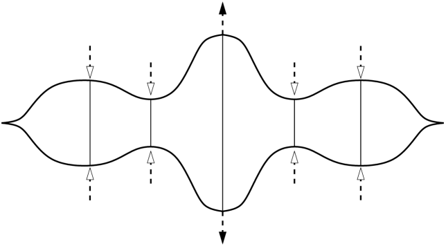
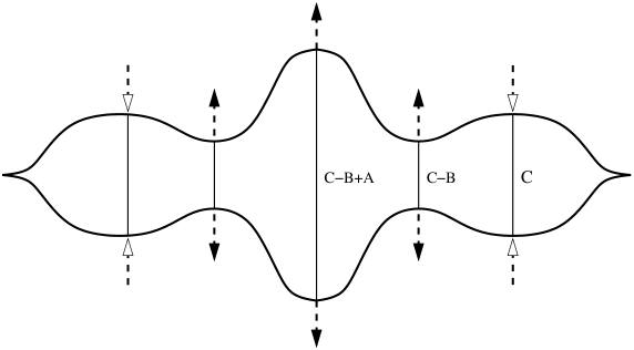
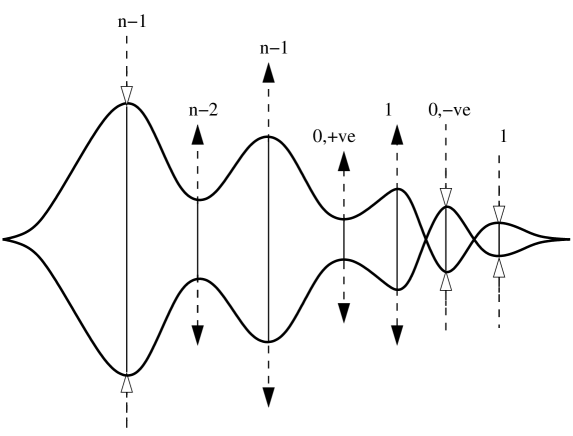
We introduce two Bott families and of slice Reeb chords of index and , respectively. Both families are topologically -spheres, symmetric about the central slice Reeb chord. The lengths of the slice Reeb chords of the families are , , and ; see Figure 2. It will be important later that is not too small compared to . We introduce the following quantities corresponding to certain areas in the Lagrangian slice projections which appear later, but here related to the lengths of the slice Reeb chords:
where and . Then , , and . To be definite about , we take and , where are parameters such that . (Since the slice Reeb chords must change length with , we cannot enforce but we can take these parameters to be approximately equal to . )
A.4.3.
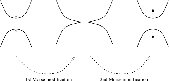
We Morse modify along the Bott family of slice Reeb chords of minimal length twice, first adding a family of 1-handles and then removing them, as shown in Figure 3. It is straightforward to check that the manifold that results from these modifications is a punctured connected sum , i.e., . The slice sphere that appears right after the second Morse modification is depicted in Figure 4.
A.4.4.
In the final step of the first piece, we Morsify the Bott family of slice Reeb chords. In doing so, as we shall see below, it is natural to think about the quantities , , and as functions of , where we think of as the unit sphere , which naturally parameterizes the Bott manifold. We Morsify leaving one very short chord with lying in direction and one long chord in direction , with
| (A.2) |
see Figure 4. Here, is as above, and is constant in since we keep the Bott symmetry of . The superscripts on and refer to the Morse indices of the slice Reeb chords, considered as positive function differences of the functions defining the two sheets of the front at their endpoints.
Let be such a positive difference between local functions defining the sheets of the front. For future reference, we assume that the Morsification has only a small effect on the level surfaces of , which remain close to those of the Bott situation. In particular, the level curves of for values close to are everywhere transverse to the radial vectors along an slightly outside the former Bott-manifold, see Figure 5.
A.5. A guide to reading pictures of Lagrangian slices
For the next three pieces of the immersion, we will not use the front representation as above, but will instead draw a family of exact Lagrangian slices. Before reaching the details we describe how to read the pictures.
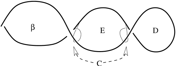
Let and let . We construct our exact Lagrangian slice-spheres by drawing their slices in the -dimensional half-planes determined by and its dual vector , i.e. is a vector in -space dual to which lies in -space. These slices are curves that begin and end at a central point (the location of the slice Reeb chord of maximal length of the corresponding front) at . In order for the curves to close up and form a sphere, the integral must be independent of .
We will draw the immersed curves with over/under information recording the value of the -coordinate at double points. It is also important to keep track of the values of at crossings, where is a primitive function of the exact Lagrangian slice. We write and for the differences in -coordinate and -coordinate, respectively, between the upper and the lower strands at the crossing labeled in figures. Note that with these conventions .
We next need a description of the actual double points of the slice immersions in terms of the curves . Note first that any double point of corresponds to a double point of some curve . Although we break the symmetry we stay fairly close to a symmetric situation. In particular, the double points of the curves (with the exception of the central double point) will come in -families and the -differences then give functions
Since double points correspond to parallel tangent planes on the front we find that the double points of are exactly the critical points of these functions.
A.6. The second piece of the immersion
We will represent the second piece of the immersion in three steps.
A.6.1.
In the initial step the curves correspond to the front in Figure 4, which is depicted in the slice model in Figure 6. , , and denote the (positively oriented) areas indicated; each is a function of and . We then have
In particular and, for fixed , the functions and have maxima at and minima at , whereas the function is constant in .

A.6.2.
We apply a finger move across the area , splitting it into two pieces and as shown in Figure 7, where is constant in :
Consequently, equals .
The crossing conditions then read:

A.6.3.
We continue the finger move and introduce a new small area , as shown in Figure 8. We have
| (A.3) | ||||||
| (A.4) | ||||||
| (A.5) | ||||||
| (A.6) | ||||||
| (A.7) |

A.7. The third piece of the immersion
The slices of the third piece will be drawn in the same way as the slices in Section A.6. We will distinguish small and large deformations, and use for quantities that are almost constant in time, and for those that are almost constant in both and in time. Recall that we wrote for the height of the smallest Reeb chord, where ; by a small deformation we mean one smaller than for . For example means that the area is independent of and that it has -derivative of order , , with the sign of the derivative dictated by the crossing conditions.
A.7.1.
In the initial phase of the third piece we change the area functions in such a way that the following conditions are met:
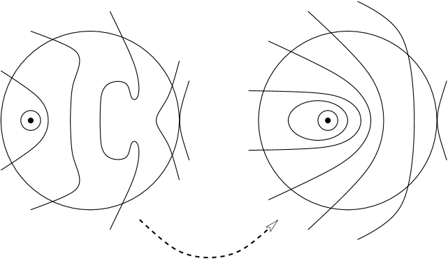
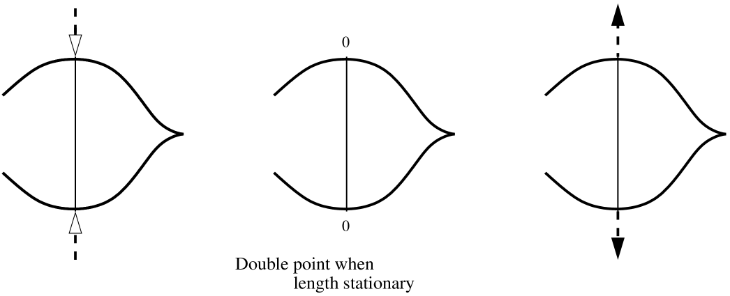
where is the starting time. Consider as above. At , the values of all area functions stay close to their initial values. At , shrinks toward and grows correspondingly. We choose these functions so that they have exactly two critical points . Note that these deformations are compatible with (A.3)–(A.7). At the point when we find that the central slice Reeb chord which corresponds to a maximum of the function difference determined by the two sheets of the front and to the double point labeled cancels with the chord corresponding to the largest value of . The curve at the cancelling moment is depicted in Figure 9.

Note that at this point the slice Reeb chord that corresponds to the double point labeled satisfies the following:
| (A.8) |
where we recall that and that denotes the initial instance, before we start shrinking , see Step 4. In particular, the Reeb chord of maximal length is the chord labeled (denoted earlier) of length .
A.7.2.
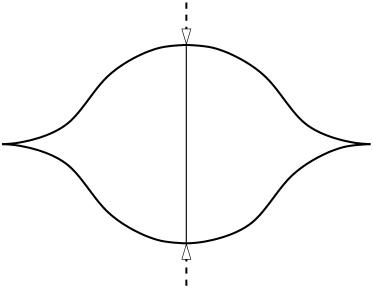
In the central region where the Reeb chords cancel, the front of the Lagrangian slice consists of two function graphs. The level sets of the positive difference of these function graphs are shown in Figure 10.
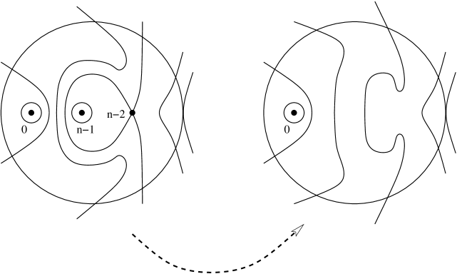
Recall the consequence of the earlier Bott set up, see Step 4, that the level sets are transverse to the radial vectors along an surrounding the central region. Thus isotoping level sets keeping them fixed along the boundary, we see that there exists a Hamiltonian isotopy which is fixed outside the central region that deforms the Lagrangian so that the central region appears as shown in Figure 11. Here the slice Reeb chord is the new central Reeb chord and level sets are everywhere transverse to the radial vector field. Noting that double points in the central region of the radial slices correspond to tangencies of the level sets and the radial vector field, we find that after this Hamiltonian deformation, the curves are as shown in Figure 12. We take the slices of our exact Lagrangian to be approximately equal to the instances of this Hamiltonian deformation, deviating from it slightly in order to ensure that the crossing conditions hold.

We have the following crossing conditions:
| (A.9) | ||||||
| (A.10) | ||||||
| (A.11) | ||||||
| (A.12) |
For the deformation described above, the function in Figure 12 has only two critical points, with maximum value at :
| (A.13) |
and minimum value at :
| (A.14) |
A.8. The fourth piece of the immersion
We describe the fourth piece in four steps.
A.8.1.
We rotate the ends of the curves as shown in Figure 13. More precisely, recall that are coordinates on the half plane in which lies. Consider an interval and small, such that (i) all curves are of standard form in , and (ii) all curves are contained in . Consider a Hamiltonian deformation that is constant in , that is a rotation in the region , and that is again constant in . The curves are then given by small deformations of the curves ; the small deformations shrink the areas and , and increase the area , in each case with very small derivative, in order to have the crossing conditions satisfied.

A.8.2.
We shrink the area for in a certain subset of . Recall from Equations (A.13),(A.14) that the minimum of the function is whereas its maximum . Consider the subset where
Over we shrink and in such a way that until . Outside a neighborhood of we keep at its original size. Note that outside we have
| (A.15) |
A.8.3.
We slide out across without creating double points. To see that this is possible we subdivide into three cases. First, around , is small (size ) compared to , which is of (order ) finite size. In this case there are two double points created when enters and leaves , see Figure 14. The crossing conditions at the entering crossings read
and those at the exiting crossings
where . Here we let and we let shrink to keep the above derivative positive. As the total variation of (i.e. the total amount of area transported in and out of ) is and since , is sufficiently large to keep the derivative positive at all times.
Second, well outside a neighborhood of , is large and there are two double points throughout the deformation, see Figure 15, where the crossing conditions read
where and where . Here and we ensure that the crossing conditions hold by shrinking . Since the total variation of is at most the area and in this region, we find that the crossing condition is met at all times.
Third, in the region where we interpolate between small and large , is already smaller than , and the amount of area transported through is smaller than the corresponding amount described above; hence the necessary crossing conditions can be arranged by shrinking . In conclusion we can thus slide out for all .

A.8.4.
The final stage of the fourth piece is shown as a Lagrangian slice in Figure 16 and as the corresponding front in Figure 17. The latter serves as the starting point of the last piece.

A.9. The fifth piece of the immersion
For the fifth, final piece of the immersion, we return to the front representation. The initial front of the fifth piece is a sphere with seven Reeb chords, see Figure 17, three that shrink and four that grow. It is the double of a function graph with critical points as follows: (i) the largest maximum is positive and shrinking; (ii) there is another positive local maximum that increases; (iii) one positive index point increases; (iv) there are two positive index chords, one increasing and one decreasing; (v) and there are two index chords, one positive increasing and one negative decreasing.
We pass the decreasing index chord through a double point, making it increasing, see Figure 18. Then we cancel the two index pairs and the index pair of increasing chords. This leaves us with a standard sphere, with a decreasing slice Reeb chord corresponding to a maximum, that we cap off with a Lagrangian disk via a standard Morse modification; see Figure 19. This completes the construction of the desired exact Lagrangian immersion with one double point.
References
- [1] Asadi-Golmankhaneh, M. and Eccles, P. Double point self-intersection surfaces of immersions. Geom. Topol. 4 (2000), 149–170.
- [2] Audin, M. Fibrés normaux d’immersions en dimension double, points doubles d’immersions lagragiennes et plongements totalement réels. Comment. Math. Helv. 63 (1988), no. 4, 593–623.
- [3] Bourgeois, F., Ekholm, T., and Eliashberg, Y. Effect of Legendrian surgery. Geom. Topol. 16 (2012), no. 1, 301–389.
- [4] Cieliebak, K. and Eliashberg, Y. From Stein to Weinstein and back. Symplectic geometry of affine complex manifolds. American Mathematical Society Colloquium Publications 59. American Mathematical Society, Providence, RI, 2012.
- [5] Damian, M. Floer homology on the universal cover, a proof of Audin’s conjecture, and other constraints on Lagrangian submanifolds. Comment. Math. Helv. 87 (2012) 433–462.
- [6] Ekholm, T., Etnyre, J., and Sabloff, J. A duality exact sequence for Legendrian contact homology. Duke Math. J. 150 (2009), no. 1, 1–75
- [7] T. Ekholm, J. Etnyre and M. Sullivan, Non-isotopic Legendrian submanifolds in , J. Differential Geom. 71 (2005), 85–128.
- [8] Ekholm, T., Etnyre, J., and Sullivan, M. Orientations in Legendrian contact homology and exact Lagrangian immersions. Internat. J. Math. 16 (2005), no. 5, 453–532.
- [9] Ekholm, T. and Smith, I. Exact Lagrangian immersions with a single double point. Preprint, arXiv:1111.5932.
- [10] Ekholm, T. and Smith, I. Exact Lagrangian immersions with one double point revisited. Preprint, arXiv:1211.1715.
- [11] Y. Eliashberg, Topological characterization of Stein manifolds of dimension . Internat. J. Math. 1 (1990), 29–46.
- [12] Y. Eliashberg and M. Gromov, Lagrangian intersection theory: finite-dimensional approach. In Geometry of differential equations, Amer. Math. Soc. Transl. Ser. 2, 186, (1998), 27–118.
- [13] Eliashberg, Y. and Murphy, E. Lagrangian caps Preprint, 2013.
- [14] K. Fukaya. Application of Floer homology of Lagrangian submanifolds to symplectic topology. In Morse theoretic methods in nonlinear analysis and in symplectic topology, 231-276, NATO Sci. Ser. II Math. Phys. Chem. 217, Springer (2006).
- [15] K. Fukaya, Y.-G. Oh, H. Ohta and K. Ono. Lagrangian intersection Floer theory: anomaly and obstruction. Part I. American Mathematical Society, International Press (2009).
- [16] Gromov, M. Partial differential relations. Ergebnisse der Mathematik und ihrer Grenzgebiete (3) 9 Springer-Verlag, Berlin (1986).
- [17] Gromov, M. Pseudoholomorphic curves in symplectic manifolds. Invent. Math. 82 (1985), no. 2, 307–347.
- [18] E. Murphy, Loose Legendrian Embeddings in High Dimensional Contact Manifolds. Preprint, arXiv:1201.2245.
- [19] L. Polterovich. The surgery of Lagrange submanifolds. Geom. Func. Anal. 2 (1991), 198–210.
- [20] Sauvaget, D. Curiosités lagrangiennes en dimension 4. Ann. Inst. Fourier (Grenoble) 54 (2004) no. 6, 1997–2020.
- [21] C. Viterbo. A new obstruction to embedding Lagrangian tori. Invent. Math. 100 (1990), 301–320.
- [22] Whitney, H. The self-intersections of a smooth -manifold in -space. Ann. of Math. (2) 45, (1944), 220–246.