ContEvol formalism: numerical methods based on Hermite spline optimization
Abstract
We present the ContEvol (continuous evolution) formalism, a family of implicit numerical methods which only need to solve linear equations and are almost symplectic. Combining values and derivatives of functions, ContEvol outputs allow users to recover full history and render full distributions. Using classic harmonic oscillator as a prototype case, we show that ContEvol methods lead to lower-order errors than two commonly used Runge–Kutta methods. Applying first-order ContEvol to simple celestial mechanics problems, we demonstrate that deviation from equation(s) of motion of ContEvol tracks is still ( is the step length) by our definition. Numerical experiments with an eccentric elliptical orbit indicate that first-order ContEvol is a viable alternative to classic Runge–Kutta or the symplectic leapfrog integrator. Solving stationary Schrödinger equation in quantum mechanics, we manifest ability of ContEvol to handle boundary value or eigenvalue problems. Important directions for future work, including mathematical foundation, higher dimensions, and technical improvements, are discussed at the end of this article.
keywords:
Computational methods (1965)1 Introduction
Numerical simulations are widely used in contemporary physics. For instance, famous computer codes in astrophysics include Arepo (Springel, 2010) and Athena++ (Jiang et al., 2014) for (magneto)hydrodynamic simulations, galpy (Bovy, 2015) for galactic dynamics, YREC (Demarque et al., 2008) and MESA (Paxton et al., 2011) for stellar evolution, mercury (Chambers, 1999) and REBOUND (Rein and Liu, 2012) for celestial mechanics, to name a few. There are certainly great works in other areas of research as well.
Because of the discreteness of the world of computers, it is common practice to convert differential equations into difference equations, so that finite difference methods can be applied. However, at spatial scales much larger than elementary particles, the physical world is arguably continuous. Therefore, finite difference might be intrinsically limited: when we try to model the full history of a dynamic system or full details of a function of spatial location, we have to resort to spline interpolation. Meanwhile, many physics problems are formulated as first- or second-order differential equations with analytic expressions, indicating that usage of general-purpose methods might be an overkill. These motivate the ContEvol (continuous evolution) formalism, which we222According to context, the pronouns “we/us/our” in this work may refer to: i) the author and indirect contributors (see acknowledgements), ii) the author and researchers with similar academic background and interests, or iii) the author and the readers. present in this work.
Desire for continuity has provoked thoughts about function representation. Imaging that, in addition to values of a one-dimensional real function at a series of sampling points , we have its first derivative at the same points. Then in each interval , we can always find a cubic polynomial satisfying all boundary conditions at both ends, so that can be represented as a piece-wise cubic function — not only is it continuous, but its first derivative is also continuous, which is favorable to some analysis in physics. This technique is known as Hermite spline333Anecdote: The author “independently” came up with this idea about three weeks before hearing about Hermite spline. For this reason, the author feels obliged to declare the possibility that this work might be reinventing some methods.. It can be naturally extended to higher orders: combining values and first- to th-order derivatives at both ends of an interval, we can find a st-order polynomial representation of the function. However, it should be noted that basic calculus yields simple but powerful expressions for addition, subtraction, multiplication, division, and composition of representations with only values and first derivatives:
| (1.0.1) | |||||
| (1.0.2) | |||||
| (1.0.3) | |||||
| (1.0.4) |
Finiteness can be a blessing and a curse — we lose some high-order information, but do not need to assume that functions are infinitely differentiable, unlike when we use spectral methods (e.g., Grandclément and Novak, 2009).
ContEvol is a family of numerical methods built on this idea. It approximates functions of space and time as polynomials and minimizes deviation from equation(s) of the problem. While details will be presented and discussed in the rest of this work, here we briefly address how this relates to other common methods (e.g., Press et al., 2007). Some of the most important dichotomies of numerical methods include: explicit or implicit, single-step or (linear) multistep, and symplectic (or in physicists’ words, phase space conserving) or not. Since ContEvol finds the optimal solution for the next step, it should be categorized as implicit; however, as we will show in this work, unlike common implicit methods, ContEvol only needs to solve linear equations. Although this work focuses on the single-step version of ContEvol, we will argue that multistep versions are straightforward to achieve. Because of the predefined functional form, ContEvol is not strictly symplectic; however, with moderately small steps, its non-symplecticity (deviation from of determinant of Jacobian) can be rapidly below , i.e., inundated by roundoff errors of double precision.
This work is principally for illustration and discussion of general strategies. The rest of this article is structured as follows. In Section 2, we apply first- and second-order ContEvol methods444An th-order ContEvol method treats up to th-order derivatives at sampling nodes as independent variables. to a prototype case, classic harmonic oscillator, and compare them to fourth- and eighth-order Runge–Kutta methods. Then in Section 3, we showcase potential applications of ContEvol in celestial mechanics; examples in this work are two-body and three-body problems, in which equations of motion are non-linear and multivariate. In Section 4, we use ContEvol to solve stationary Schrödinger equation in quantum mechanics, which is physically different from time evolution of a dynamic system. Finally in Section 5, we wrap up this work by discussing important directions for future work, including mathematical foundation, higher dimensions, and technical improvements.
2 Prototype case: classic harmonic oscillator
We start with the simplest case of a dynamical system: time evolution of a single real variable. To check results of numerical methods against exact solution, we choose the classic harmonic oscillator, for which the equation of motion (EOM) is
| (2.0.1) |
where is the mass of the particle and is the spring constant; setting these constants to 555This is a natural choice which makes time dimensionless. A different scaling would lead to different cost functions and thus different optimization results, but is not explored in this work., the EOM becomes
| (2.0.2) |
Without loss of generality, we are given , and try to solve for , , where is the time step (usually small). The exact solution is
| (2.0.3) |
Section 2.1 showcases ability of the first-order ContEvol method, and Section 2.2 compares it to two commonly used (explicit and multistep) Runge–Kutta methods. In Section 2.3, we explore the second-order ContEvol method, with and without strict EOM enforcement at .
2.1 First-order ContEvol method
We approximate the solution in a parametric form (subscript “CE1” stands for first-order ContEvol)
| (2.1.1) |
“terminal” conditions at yield
| (2.1.2) | ||||
| (2.1.3) | ||||
| (2.1.4) |
Because of the initial conditions , the transformation is affine, not linear.
We define the cost function as
| (2.1.5) |
minimizing this, we obtain
| (2.1.6) | ||||
| (2.1.7) | ||||
| (2.1.8) |
The determinant of the time evolution operator is
| (2.1.11) |
i.e., unfortunately, ContEvol is not symplectic. However, the discrepancy (common double-precision floating-point format cannot tell discrepancies below this threshold) when . Thanks to the linearity of the problem, is diagonalizable for common choices of , and complexity of evolving the system for steps with fixed time step can be just .
Expanding Eqs. (2.1.9) and (2.1.10), first-order ContEvol yields
| (2.1.12) |
comparing to the exact solution Eq. (2.0.3), we see that errors in and (highlighted in red) are and , respectively.
According to Eq. (2.1.8), the minimized cost function Eq. (2.1) is
| (2.1.13) |
note that seems consistent with . This minimization goal can be used to adapt step length, e.g., for and ( and ), 666In this section, we use as a general-purpose benchmark for numerical precision, although it is only a threshold for double-precision when the leading-order term is . when ().
2.2 Fourth- and eighth-order Runge–Kutta methods
To enable Runge–Kutta methods, the equation of motion Eq. (2.0.2) has to be written as
| (2.2.1) |
Like in many physics problems, this derivative does not have explicit time dependence.
Applying the fourth-order (i.e., classic) Runge–Kutta method, we have
| (2.2.2) | ||||
| (2.2.3) | ||||
| (2.2.4) | ||||
| (2.2.5) |
and then
| (2.2.6) |
Evidently, errors in and are both .
The determinant of the time evolution operator is
| (2.2.7) |
i.e., the discrepancy is two orders larger than ; to archive , one needs , times smaller than what was required for first-order ContEvol. To adapt step length, the fourth-order Runge–Kutta method usually resorts to the fifth-order version, which necessitates a slight increase in computational complexity.
Now let us try the eight-order Runge–Kutta method777RK8 coefficients used in this work are found on the MathWorks webpage “Runge Kutta 8th Order Integration”: https://www.mathworks.com/matlabcentral/fileexchange/55431-runge-kutta-8th-order-integration., which gives (subscripts “RK8” on the right-hand side are omitted for simplicity)
| (2.2.8) | ||||
| (2.2.9) | ||||
| (2.2.10) | ||||
| (2.2.11) | ||||
| (2.2.12) | ||||
| (2.2.13) | ||||
| (2.2.14) | ||||
| (2.2.15) | ||||
| (2.2.16) | ||||
| (2.2.17) |
and then
| (2.2.18) |
For some unknown reason, the fourth-order coefficients have a fractional error of , while the fifth- to eighth-order coefficients agree with the exact solution Eq. (2.0.3).
The determinant of the time evolution operator is
| (2.2.19) |
to archive , one needs , times smaller than what was required for fourth-order Runge–Kutta.
2.3 Second-order ContEvol method
The ContEvol framework can be naturally generalized to higher orders. Like in Section 2.1, we approximate the solution in a parametric form (subscript “CE2” stands for second-order ContEvol)
| (2.3.1) |
“terminal” conditions at yield
| (2.3.2) | ||||
| (2.3.3) | ||||
| (2.3.4) |
Note that we have enforced the EOM at both and , and the three coefficients (, , and ) are fully specified by two parameters ( and ).
Likewise, we define the cost function as
| (2.3.5) |
minimizing this, we obtain
| (2.3.6) | ||||
| (2.3.7) | ||||
| (2.3.8) |
Option 1: With EOM enforced at (“direct” solution).
First, we enforce by rewriting the cost function Eq. (2.3) as
| (2.3.9) |
minimizing this, we obtain (“d” in the subscript stands for direct)
| (2.3.10) | ||||
| (2.3.11) | ||||
| (2.3.12) |
or equivalently
| (2.3.13) |
with
| (2.3.14) |
The determinant of the time evolution operator is
| (2.3.15) |
to archive , one only needs , times larger than what was required for first-order ContEvol.
Expanding Eqs. (2.3.13) and (2.3.14), second-order ContEvol with enforced yields
| (2.3.16) |
comparing to the exact solution Eq. (2.0.3), we see that errors in and (highlighted in red) are still and , respectively, same as first-order ContEvol Eq. (2.1.12); however, the coefficients are much closer to the exact values.
Option 2: Without EOM enforced at (“indirect” solution).
Second, we remove the constraint and simply adopt Eq. (2.3.8); ergo (“i” in the subscript stands for indirect)
| (2.3.18) |
or equivalently (neglecting the acceleration; note that this “indirect” strategy automatically avoids accumulation of additional error in , as it “resets” to at each step)
| (2.3.19) |
with
| (2.3.20) |
The determinant of the time evolution operator is
| (2.3.21) |
to archive , one needs , times smaller than what was required when we enforce .
Expanding Eqs. (2.3.19) and (2.3.20), second-order ContEvol without the constraint yields
| (2.3.22) |
comparing to the exact solution Eq. (2.0.3), we see that errors in and (highlighted in red) are once again and , respectively. Note that the “indirect” coefficients Eq. (2.3.22) are slightly closer to the exact version than their “direct” counterparts Eq. (2.3.16).
According to the optimal coefficients Eq. (2.3.8), the minimized cost function Eq. (2.3) is
| (2.3.23) |
when (), for and ( and ).
To summarize, the marginal benefit of raising ContEvol to second order is moderate: this reduces the minimized cost function from to — leading to a better representation of the evolutionary track — but does not reduce the order of errors in or . One is advised to enforce equation of motion at if symplecticity is more important, but to remove this constraint if error control takes priority. In the rest of this work, we only consider first-order ContEvol methods, as for real-world problems, second derivatives might be unavailable or unaffordable.
3 Celestial mechanics: two-body and three-body problems
In this section, we extend the ContEvol framework to time evolution of multiple real variables. As astrophysicists, we choose two simplest cases from celestial mechanics, two-body and three-body problems.
The equations of motion (EOMs) for a two-body problem are
| (3.0.1) |
where is the gravitational constant and denotes masses of the two objects; setting the constant to , these can be straightforwardly reduced to
| (3.0.2) |
with and 888In the rest of this section, we use regular symbols to denote magnitudes of vectors without further notice.. This problem only needs to be solved in two dimensions, as the particle never leaves the plane spanned by initial conditions — or the line, if the initial position and velocity are collinear, but it is trivial to apply full results to the one-dimensional case. The general solution to the above EOM can be expressed in parametric forms, which we do not include here; exact solutions to specific problems (i.e., for specific initial values) will be presented when needed.
The (unrestricted) three-body problem is more complicated, with equations of motion
| (3.0.3) |
where the prime “′” denotes inertial coordinate system; writing , and , for , these equations can be reduced to
| (3.0.4) |
The above equations do not have a closed-form solution in general.
Although and will be written as polynomials, Taylor expansion of has infinitely many terms, hence some truncation is necessary. In Section 3.1, we apply first-order ContEvol method to the two-body problem, keeping “adequately” many terms. We show that this is equivalent to linearization and Taylor expansion in Section 3.2. In Section 3.3, we investigate conservation of mechanic energy and angular momentum, before moving on to numerical tests with an eccentric elliptical orbit in Section 3.4. Finally in Section 3.5, we describe how ContEvol is supposed to be applied to the three-body problem.
3.1 Two-body, first-order ContEvol with “adequate” expansion
Without loss of generality, we are given , and try to solve for , , where is the time step. Like in Section 2.1, we approximate the solution in a parametric form (subscript “CE2” now stands for ContEvol and two-body problem; note that we are recycling the subscripts)
| (3.1.1) |
with coefficients and yielded by “terminal” conditions at
| (3.1.2) |
To define the cost function as a finite polynomial of , we have to truncate the Taylor expansion on the right-hand side of the EOM Eq. (3.0.2). Since traces up to the third order, we do not expect any benefit from going beyond the third order; justifying this statement is left for future work — note that non-linear coefficients in and start to occur at the fourth order, so one would have to solve non-linear equations to minimize the cost function. Thus we have
| (3.1.3) |
and the cost function is defined as
| (3.1.4) |
with
| (3.1.5) |
because of the , , and terms, the two components are coupled with each other.
Minimizing this, we obtain
| (3.1.6) |
where we have omitted some high-order terms (“”; up to ) for simplicity, and equations and as they can be easily obtained via swapping subscripts and ; because of the coupling mentioned above, there are cross terms in high-order coefficients.
Put in matrix form, the system of equations is
| (3.1.7) |
with
| (3.1.8) |
and
| (3.1.9) |
the solution999To prevent Wolfram Mathematica from taking forever, one is advised to keep only up to (or another desired order) terms at each step. This advice also applies to computation of determinant of the Jacobian matrix in this case. is
| (3.1.10) |
where again we have omitted some high-order terms (up to ) and expressions for components.
Plugging Eq. (3.1.10) back into Eq. (3.1.1), our solution at is
| (3.1.11) |
thus the Jacobian matrix is
| (3.1.12) |
with
| (3.1.13) | ||||
| (3.1.14) | ||||
| (3.1.15) | ||||
| (3.1.16) |
Note that “symmetries” in the Jacobian are broken at high orders. Its determinant is
| (3.1.17) |
i.e., the non-symplecticity is at the level, three orders larger than applying first-order ContEvol to classic harmonic oscillator (see Section 2.1, specifically Eq. (2.1.11)).
According to Eq. (3.1.10), the minimized cost function Eq. (3.1) is
| (3.1.18) |
the order in is same as in the prototype case Eq. (2.1.13); however, when is small, i.e., when , the above expression can still be large.
Test case 1: Uniform circular motion.
Consider the initial conditions and . The particle will perform a uniform circular motion along the unit circle.
The exact solution is (subscript “UCM” stands for uniform circular motion)
| (3.1.19) |
while first-order ContEvol with “adequate” expansion yields
| (3.1.20) |
i.e., like in Section 2.1, errors in and (highlighted in red) are and , respectively.
Test case 2: Parabolic motion.
Consider the initial conditions and . The particle will move along the parabola .
According to conservation of angular momentum and mechanic energy (see Section 3.3 for further treatment), the exact solution is (subscript “PBM” stands for parabolic motion)
| (3.1.21) |
where is within the radius of convergence for the expansion, and
| (3.1.22) |
First-order ContEvol with “adequate” expansion yields
| (3.1.23) |
Again, errors in and (highlighted in red) are and , respectively.
3.2 Two-body, equivalence with linearization and Taylor expansion
In this section, we show that first-order ContEvol with “adequate” expansion is equivalent to both linearization and fifth-order Taylor expansion of the equation of motion.
Equivalence with linearization.
An alternative way to handle the right hand side of the EOM Eq. (3.0.2) is to define
| (3.2.1) |
and use its derivatives at and to approximate it as (again, subscript “CE2” stands for ContEvol and two-body problem)
| (3.2.2) |
with coefficients and yielded by “terminal” conditions at
| (3.2.3) |
Evidently, we have (see Eq. (3.1.5) for , ).
Since only depends on time through , its derivative is
| (3.2.4) |
where we have used Einstein notation. Similarly, we have .
The coefficients and can be fully specified by either and (see Eq. (3.1.2)) or and . Proceeding with and , the function at is
| (3.2.5) |
and its derivative at is
| (3.2.6) |
where we have “adequately” expanded and to keep all the terms without non-linear coefficients in and . Plugging these into Eq. (3.2.3), we obtain the simple relations and .
With the function , the cost function is defined as (here the prime “′” denotes linearization)
| (3.2.7) |
Therefore, linearization is equivalent to “adequate” expansion (see Section 3.1); nevertheless, this approach should be more suitable when the function does not have a simple expression, e.g., when it has to be numerically computed by interpolating in lookup tables.
Equivalence with Taylor expansion.
By successively differentiate the equation of motion Eq. (3.0.2), one can attain the third derivative (jerk)
| (3.2.8) |
the fourth derivative (snap)
| (3.2.9) |
and the fifth derivative (crackle)
| (3.2.10) |
of the position vector ; using these derivatives, the Taylor expansion of the EOM is
| (3.2.11) |
It is verified that the first-order ContEvol solution Eq. (3.1.11) is identical to
| (3.2.12) |
note that the term of is missing. Therefore, at least for the two-body problem, first-order ContEvol is equivalent to fifth-order Taylor expansion of the EOM in terms of position, and fourth-order in terms of velocity.
For relatively simple equation(s), successive derivatives are feasible; however, when the system is complicated, ContEvol could provide a “shortcut” to obtain fifth/fourth-order Taylor expansion of the evolution numerically. Specifically, one can compute counterparts of the coefficients Eq. (3.1.5) numerically, use them to construct a linear system like Eq. (3.1.7), and then solve it to obtain counterparts of and . In Section 3.5, we will outline how this is supposed to be done for the three-body problem.
The procedure described above is not the only way to implement a ContEvol method. For relatively simple problems like the two-body problem, one can choose to directly use expressions for results at , e.g., and Eq. (3.1.11). We refer to the two strategies as implementation by optimization process and implementation by optimization results, respectively. In Section 3.4, while implementing first-order ContEvol for an eccentric orbit, we will adopt the second strategy, i.e., directly utilize Eq. (3.2.12), truncating it at for and for .
3.3 Two-body, conservation of mechanic energy and angular momentum
As mentioned in the second test case of Section 3.1, two quantities should be conserved in the two body problem: mechanic energy and angular momentum. In terms of and , these are
| (3.3.1) |
respectively; note that in the case of a two-body problem, hence we only need to track its component. The proofs are straightforward:
| (3.3.2) |
where we have used the equation of motion Eq. (3.0.2) in both.
Using these two conservation laws, we can express in terms of as
| (3.3.3) |
where is the sign function, or
| (3.3.4) |
with
| (3.3.5) |
One should not use to simplify Eqs. (3.3.3) or (3.3.4), as is what we are trying to derive.
To resolve the ambiguity of the symbols, we write and as
| (3.3.6) |
and derive and from initial conditions and
| (3.3.7) |
Note that for this purpose, we are treating each pair of and as and ; in other words, we imagine an infinitesimal next step for any given position and velocity.
Plugging these into and expanding Eq. (3.3.3), we obtain
| (3.3.8) |
where we have used to simplify notation, and a similar expression for ; in the limit , we should have , and thus
| (3.3.9) |
Since , the symbols in Eq. (3.3.3) should take the same sign as .
The symbols in Eq. (3.3.4) can be determined in the same way, and the final expressions are the same. In conclusion, based on the conserved quantities and , unambiguous expression for in terms of is
| (3.3.10) |
where the prime “′” for will be explained later in this section. Note that the condition is always satisfied unless , which reduces the two-body problem to its one-dimensional case and is usually not of interest, except for calculating the “free-fall” timescale.
Similarly, we can express in terms of as
| (3.3.11) |
or
| (3.3.12) |
with
| (3.3.13) |
Plugging Eqs. (3.3.6) and (3.3.7) into and expanding Eq. (3.3.11), we obtain
| (3.3.14) |
where again we have used to simplify notation, and a similar expression for ; in the limit , we should have , and thus
| (3.3.15) |
Since , symbols in Eq. (3.3.11) should take the same sign as .
The symbols in Eq. (3.3.12) can be determined in the same way, and the final expressions are the same. In conclusion, based on the conserved quantities and , unambiguous expression for in terms of is
| (3.3.16) |
The condition is also always satisfied unless .
Admittedly, should not appear when we express in terms of , neither vice versa. Fortunately, numerical methods (including Runge–Kutta, ContEvol, etc.) usually predict both and after each time step, hence when we use (or ) to derive (or ), (or ) provided by the original numerical methods can be treated as a reasonable initial guess; these are denoted with a prime “′” in Eqs. (3.3.10) and (3.3.16).
Behavior of the sign function near zero is worth more discussion. When , i.e., when and are perpendicular to each other, , so that value of does not matter. Similarly, when , , so that value of does not matter either. In practice, neither nor can be exactly zero, except for initial conditions or very rare coincidences, yet we need to consider the cases where they are about zero, as wrong signs can change the direction of the history, which is undesirable. To resolve this issue, one can specify a threshold , and set the value of the sign function to when or , or make a smoother transition using, e.g., a rescaled logistic function.
In the context of ContEvol, there are two approaches to make use of these conservation laws.
Approach 1: Use to correct .
As shown in Section 3.1, errors in and of first-order ContEvol are and , respectively. Because of this difference, after each step, using to correct according to Eq. (3.3.10) could be beneficial.
To testify the usefulness of this approach, we plug given by Eq. (3.1.11) into Eq. (3.3.10) to attain a corrected version of , denoted as ; the discrepancy between uncorrected and corrected expressions is at the fifth order, hence we omit the latter here. Assuming , the corrected Jacobian matrix is (subscript “CC” stands for conservation correction)
| (3.3.17) |
where the matrix elements are the same as those given by Eqs. (3.1.13) through (3.1.15) for the first two rows, since we are using the same expressions for ; for the last two rows, they are different from those in Eqs. (3.1.14) through (3.1.16), but again, the leading orders are not affected, so we refrain from showing them here. Most importantly, the determinant of the corrected Jacobian is
| (3.3.18) |
i.e., the non-simplecticity has been reduced from (see Eq. (3.1.17)) to . However, it blows up when , in other words, when and are perpendicular to each other.
Then we take another look at test case 1 (of Section 3.1): uniform circular motion. Plugging given by Eq. (3.1.20) into Eq. (3.3.10), we obtain
| (3.3.19) |
The fractional error of fifth-order coefficient has been eliminated, as expected; those of sixth and seventh (highlighted in red) have been reduced as well. Eq. (3.3.1) tells us that the discrepancies in conserved quantities are ameliorated as well
| (3.3.20) |
i.e., deviations from conservation laws have been reduced by two orders. Note that the errors may arise from truncation, since we only kept up to terms in Section 3.1. Interestingly, errors in these two quantities are the same in both cases (before and after correction). We emphasize that, since and are derived from initial conditions, errors of the “CC” version do not accumulate.
In test case 2: parabolic motion, the corrected velocity vector is
| (3.3.21) |
the mechanic energy and the angular momentum before and after conservation correction are
| (3.3.22) |
respectively. The situation is basically the same as test case 1, except that the reduction in and errors is three orders in this case.
As indicated by Section 2.2, for Runge–Kutta methods, errors in and have the same order, hence it is probably not well-motivated to use one to correct another; nevertheless, the correction described in this section should still be able to produce better conservation.
Approach 2: Enforce conservation laws in the formalism.
Alternatively, we can try to enforce conservation of machanic energy and angular momentum in the ContEvol formalism.
Plugging our polynomial approximation Eq. (3.1.1) into and expanding Eq. (3.3.10), we obtain
| (3.3.23) |
further expansion (based on found above) yields
| (3.3.24) |
In short, the and coefficients determined in this way are simply zeroth-order terms of Eq. (3.1.10), which are not very useful. Therefore, in the context of ContEvol, conservation laws are better used for correction purposes.
To conclude this section, we briefly comment on how conservation of mechanic energy and angular momentum can be used in more realistic cases.
-
•
In galactic dynamics, when the matter distribution is axisymmetric, e.g., in the cases of some disk or elliptical galaxies, the situation is very similar to the two-body problem we consider here. Although both position and velocity of the particle are three-dimensional vectors now, mechanic energy and component of angular momentum are still conserved. Hence we can use these two constraints to correct and using all components of and — note that and do not appear in the expression of , and are usually significantly smaller (in terms of absolute values) than their counterparts in and directions.
-
•
In general relativity, mechanic energy and angular momentum are conserved at the level ( is the speed of light in vacuum), before gravitational waves enter the scene. Thenceforth, while studying orbital motion of a planet around a star (e.g., Mercury around the Sun) or a star around a supermassive black hole using ContEvol (or another method which lead to different orders in position and velocity), conservation correction may also be useful.
-
•
Back to Newtonian gravity. For a general three-body problem (see Section 3.5 for further discussion), there are twelve components in total (two particles, positions and velocities, three directions) and four conserved quantities (total mechanic energy and three components of total angular momentum). Therefore, especially in almost coplanar cases, we can use and to correct and , where is the index of particle; in a restricted three-body problem, where one of the particles is much less massive than the others, we can choose a different set of four velocity components.
-
•
For a general -body problem, there are components in total, but the number of conserved quantities are still four. Consequently, conservation laws become less and less useful as the number of particles increases. However, they are probably useful in hierarchical systems where we can still identify “important” velocity components. Further discussion on this topic is beyond the scope of this work.
The above discussion is only about the conservation laws per se. Since the ContEvol formalism promises to “recover” full evolutionary histories, when mechanic energy and angular momentum are not conserved for individual objects, in principle it allows users to perform corrections using energy-work and angular impulse-momentum theorems. To go one step further, if global sums of or components (all of which should be conserved) obtained via these theorems deviate from the initial values, it is reasonable to globally rescale such sums before correcting individual quantities. However, such corrections are computationally expensive, and are only recommended when conservation laws are crucial.
3.4 Two-body, numerical tests with an eccentric elliptical orbit
In this section, we conduct numerical experiments to compare first-order ContEvol with some other low-order methods for celestial mechanics. We choose a highly eccentric elliptical orbit for testing purposes.
Specifically, this elliptical orbit has eccentricity , semi-major axis , semi-minor axis , and focal distance . We write the equation of this ellipse as
| (3.4.1) |
so that location of the “central object,” i.e., origin of our coordinate system , is at the right focus. The mechanic energy of this orbit is (subscript “M” stands for mechanic and is added to distinguish energy from eccentric anomaly)
| (3.4.2) |
while the orbital period is given by Kepler’s third law
| (3.4.3) |
We let the particle start at the pericenter and move counter-clockwise. The vis-viva equation tells us the initial speed
| (3.4.4) |
so that the initial velocity is , and thus ( component of) the angular momentum is
| (3.4.5) |
At time , the position of our particle is given by
| (3.4.6) |
where the eccentric anomaly is related to the mean anomaly
| (3.4.7) |
by Kepler’s equation
| (3.4.8) |
which is a transcendental equation and has to be solved numerically.
The velocity can be obtained via Eq. (3.3.10) or expressed as
| (3.4.9) |
Ergo we have
| (3.4.10) |
since and , always has the same sign as , or equivalently . This relation will be used for conservation correction (see Section 3.3), since this section is dedicated to testing numerical methods, not the sign determination strategy.
For numerical tests in this work, we choose the following orbital parameters:
-
•
Eccentricity , semi-major axis , semi-minor axis , and focal distance .
-
•
Orbital period , mechanic energy , and angular momentum .
-
•
Pericenter at , where the velocity is ; apocenter at , where the velocity is .
Meanwhile, technical choices include:
-
•
Numerical methods: leapfrog integrator (which is simple but simplectic), fourth-order Runge–Kutta, and first-order ContEvol methods, without and with conservation correction. Note that all these methods have higher-order counterparts.
-
•
Total duration ; four fixed time steps: , , , and . For the two cases, we only record position and velocity every .
-
•
Programming language: Python with just-in-time compilation (see data availability). Processor information: 11th Gen Intel(R) Core(TM) i7-1165G7 @ 2.80GHz, 2803 Mhz, 4 Core(s), 8 Logical Processor(s). We do not use multiprocessing explicitly.
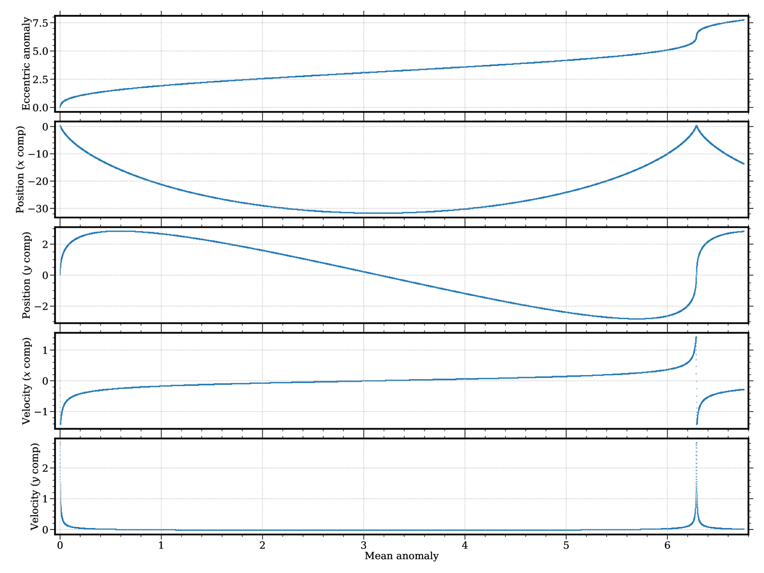
Fig. 3.4.1 displays the exact solution of this scenario. Since the particle reaches its maximum speed at the pericenter, both its position and velocity change rapidly near and . In the case of velocity near , the component reaches its maximum and quickly flips its sign, while the component reaches a larger maximum and quickly falls back. These rapid changes constitute a “stress test” for the numerical methods.
| Integrator | ||||
|---|---|---|---|---|
| LF | ||||
| LFCC | ||||
| RK4 | ||||
| RK4CC | ||||
| CE1 | ||||
| CE1CC |
Table 1 presents the time consumption of each configuration (integrator, conservation correction, and time step) tested in this work. Since the time step is fixed in each case, the time consumption is roughly inversely proportional to the time step, as expected. As a second-order method, leapfrog integrator is times faster than fourth-order Runge–Kutta; for these two methods, conservation correction increases the time consumption by a significant fraction — despite the simplicity of Eq. (3.3.10), it still takes time to perform floating point operations. Without conservation correction, first-order ContEvol costs about one half more time than fourth-order Runge–Kutta; with correction, it becomes slightly faster, since calculating from Eq. (3.3.10) is simpler than from Eq. (3.2.12). In principle, this trick can be applied to Runge–Kutta as well, but we have not explored this possibility in this work, since it would encounter more overhead and an acceleration is not guaranteed.
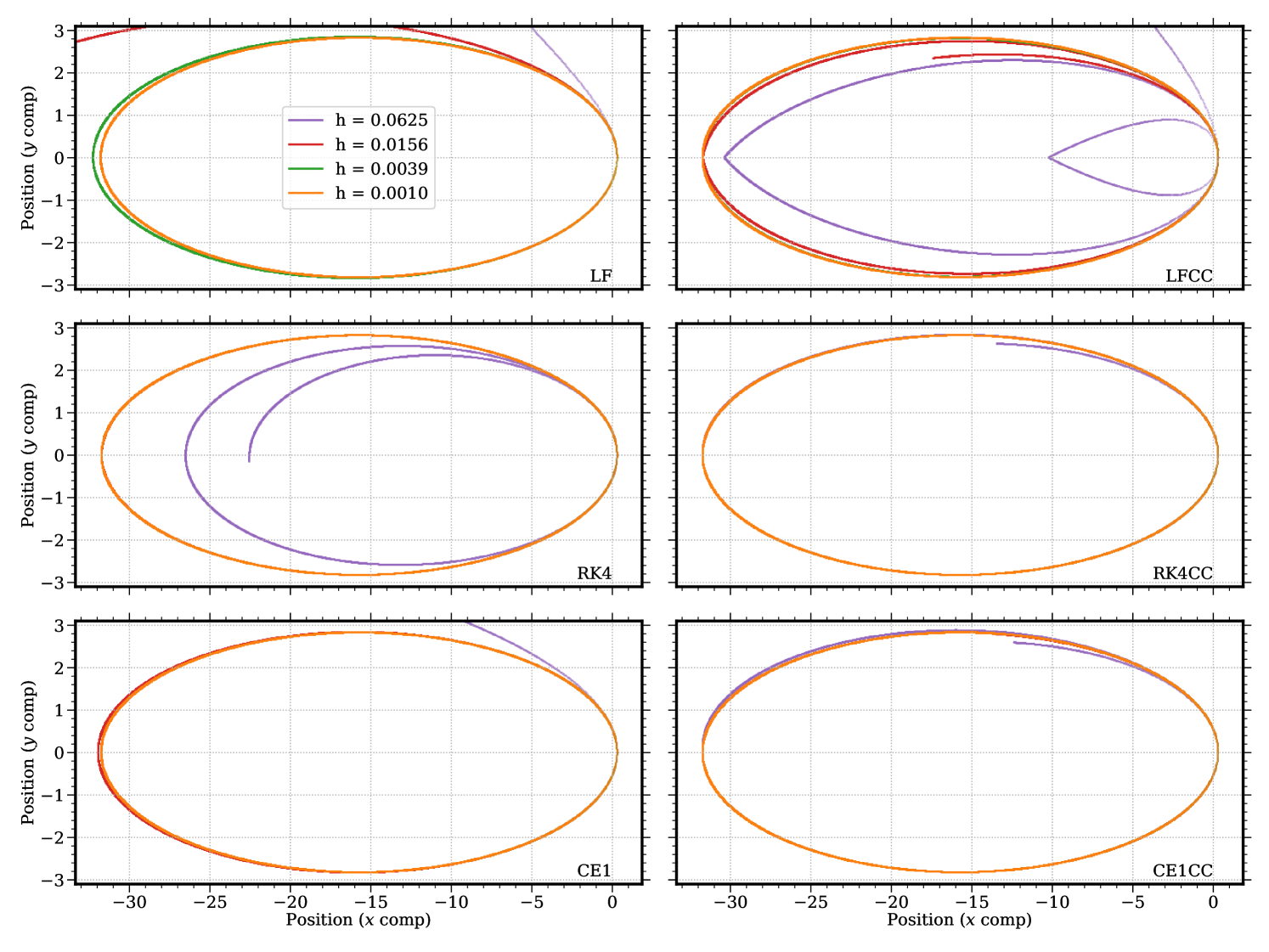
Fig. 3.4.2 shows orbits predicted by configurations tested in this work. Those close to the exact solution Eq. (3.4.6), e.g., ellipses, will be further investigated in the next few paragraphs; here we comment on significantly deviatory ones. Without conservation correction, leapfrog integrator produces a hyperbolic trajectory with , and a significantly larger and incomplete ellipse with — it only finishes slightly over half a cycle at our terminal time, . With conservation correction, the leapfrog orbit involves more artifacts, featuring two teardrop-shaped laps with different size, and then a segment of probably the third one — apparently, the correction permanently alters the history by suddenly changing the sign of ; however, the did become more reasonable. Because of their higher-order precision, fourth-order Runge–Kutta and first-order ContEvol integrators only show substantial deviations when . Without conservation correction, the Runge–Kutta orbit “loses” energy and shrinks, while its ContEvol counterpart “gains” energy and leaves the “central object.” With conservation correction, both orbits slightly flattens in the second lap, possibly due to artifacts induced by the correction, although these artifacts are less noticeable than in the case of leapfrog.
Method 1: Leapfrog integrator.
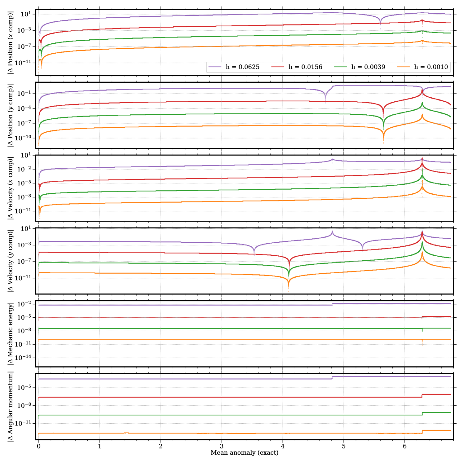
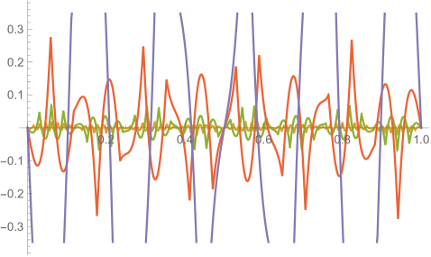
Figs. 3.4.3 and 3.4.4 display deviations from exact solution of predictions by leapfrog (“LF”) integrator without and with conservation correction (“CC”), respectively. Thanks to its symplectic nature, leapfrog (without conservation correction) conserves angular momentum remarkably well — better than both “higher-order” methods tested in this work — regardless of the time step. The mechanic energy is also well-conserved, except at the beginning , where the particle gets an “initial kick,” of which the magnitude seems proportional to the time step; nevertheless, near , none of the leapfrog orbits gets a “second kick,” making leapfrog eligible for studies of long-term (or secular) behaviors of the particle, if the energy discrepancy is acceptable. Without or with conservation correction, shrinking the time step by a factor of reduces errors in position and velocity by about an order of magnitude. However, since the correction breaks simplecticity and causes artifacts when reaches (most noticeable in the panel of Fig. 3.4.4), it only improves leapfrog in the first half of the first lap.
Method 2: Fourth-order Runge–Kutta.
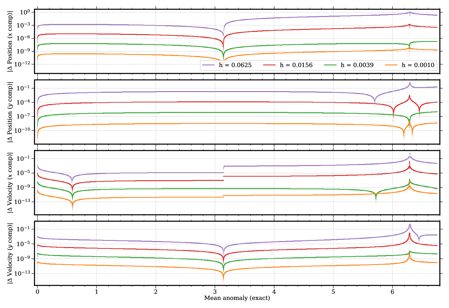
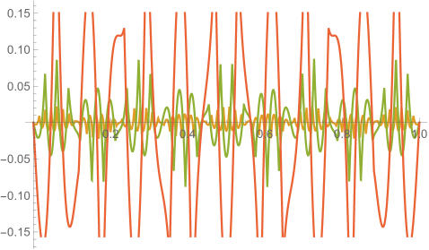
Figs. 3.4.5 and 3.4.6 display deviations from exact solution of predictions by fourth-order Runge–Kutta (“RK4”) integrator without and with conservation correction (“CC”), respectively. As a higher-order method, Runge–Kutta (without conservation correction) significantly reduces the “initial kick” (in terms of mechanic energy and angular momentum) the particle gets at ; however, the particle does get a “second kick” near , of which the amplitude shrinks with time step for mechanic energy, but is constantly about half an order of magnitude for angular momentum regardless of the time step. Therefore, quality of Runge–Kutta predictions possibly deteriorates after several laps; yet for the first lap, shrinking the time step by reduces errors by almost three (two and a half) orders of magnitude without (with) conservation correction, which is much better than leapfrog. In the first half of the first lap, with , conservation correction improves Runge–Kutta by nearly three orders of magnitude in terms of components, and almost an order of magnitude in terms of components. Because of different scaling relations described above, these improvements are slightly more significant for larger time steps; due to roundoff errors, time steps smaller than probably do not make much sense. However, a closer look at the panel of Fig. 3.4.6 would reveal a slight jump near , which is an artifact of the correction.
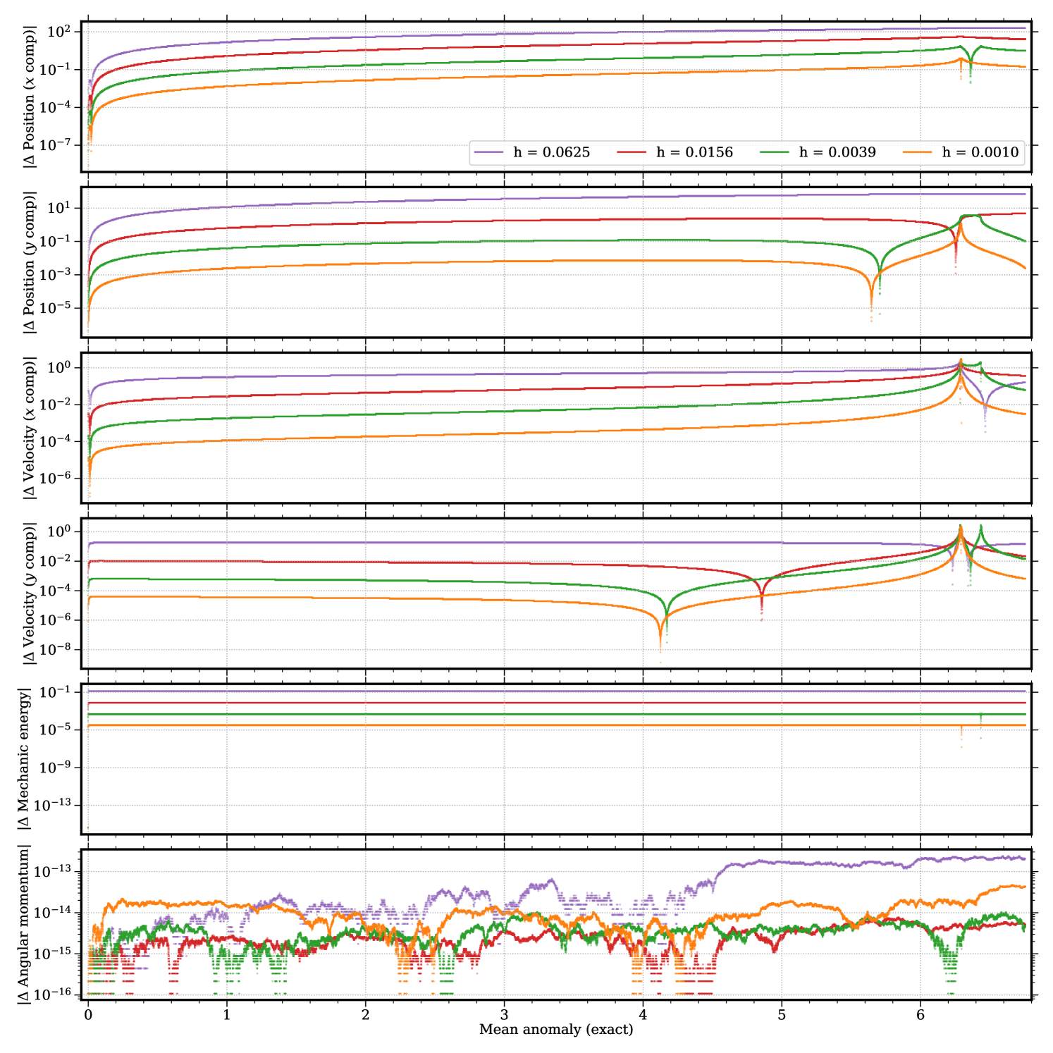
Method 3: First-order ContEvol.
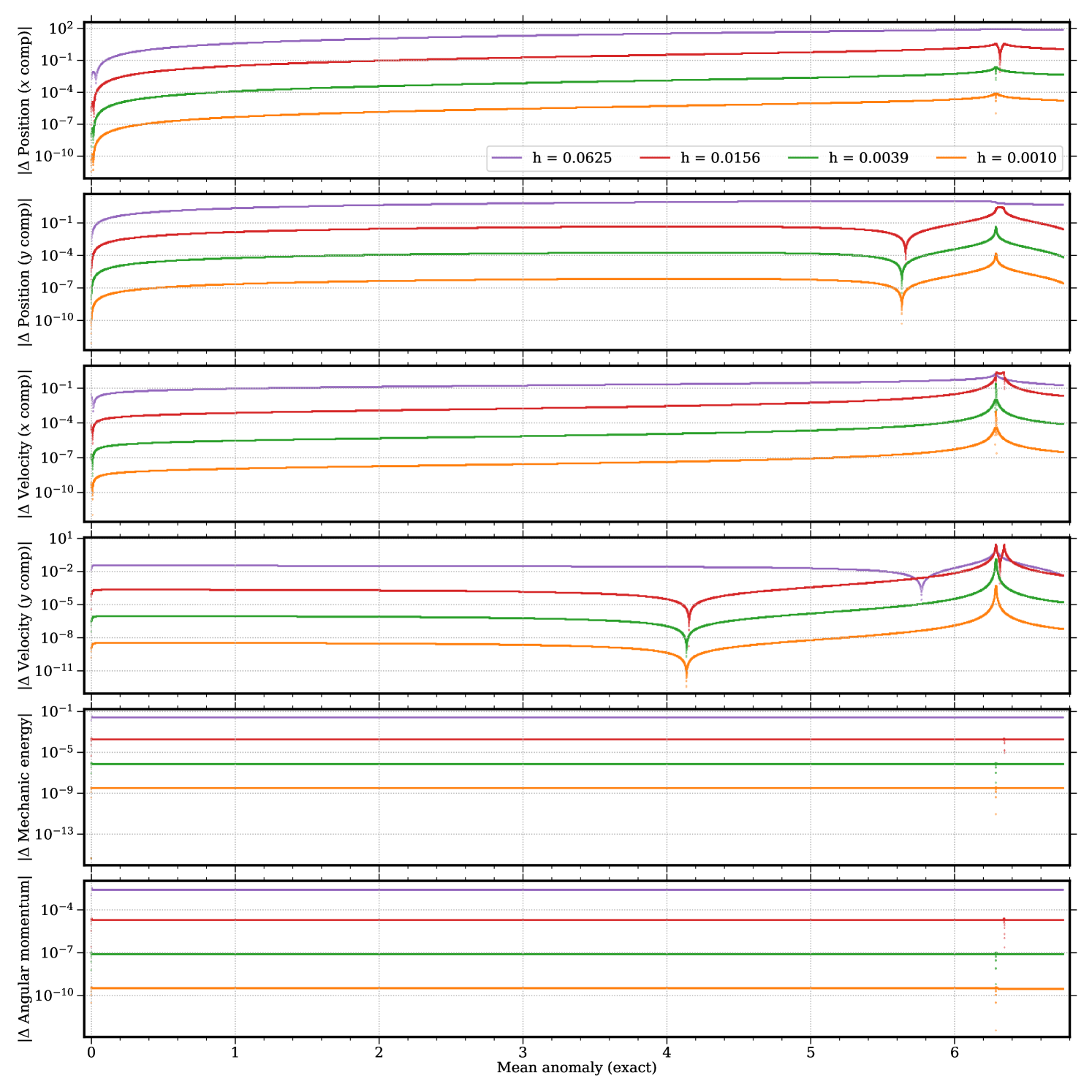
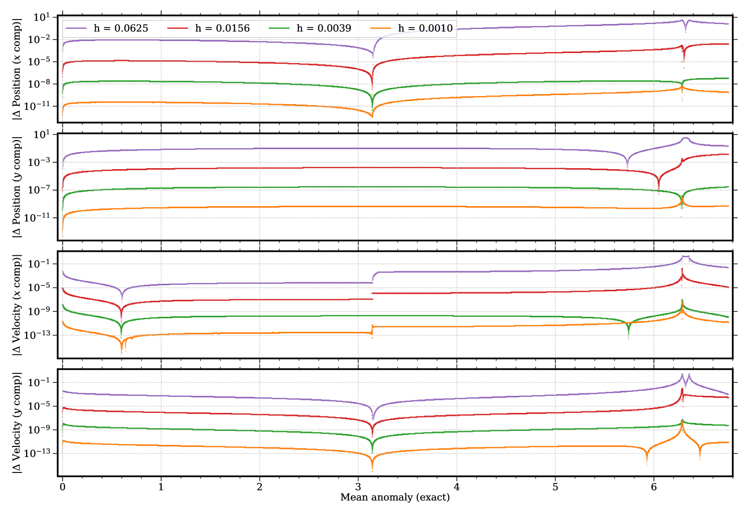
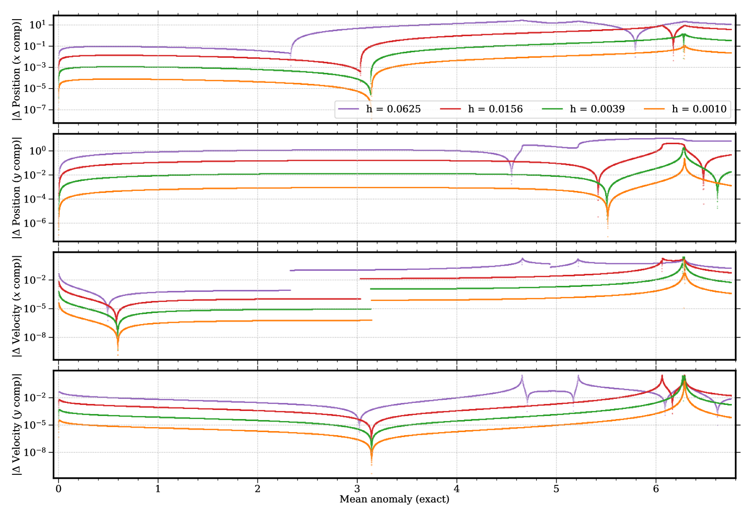
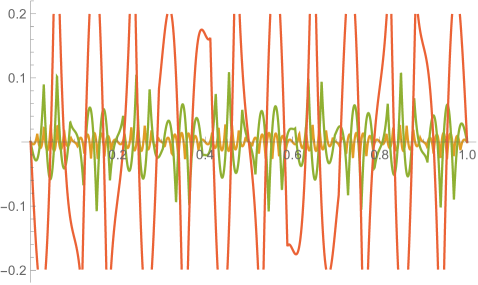
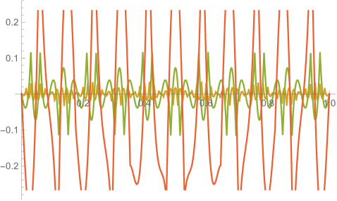
Figs. 3.4.7 and 3.4.8 display deviations from exact solution of predictions by first-order ContEvol (“CE1”) integrator without and with conservation correction (“CC”), respectively. Without conservation correction, ContEvol does not perform as well as Runge–Kutta for the first lap — the “initial kick” is almost an order of magnitude larger in terms of mechanic energy, and up to three orders of magnitude in term of angular momentum; errors in position and velocity are also about an order of magnitude larger. This is not unexpected, because although ContEvol (as implemented for these tests, see Section 3.2) accurately traces to , it only traces to , and the higher-order terms are just zero; meanwhile, Runge–Kutta accurately traces both and to , but the terms could be partially right, hence it performs better when errors accumulate. Nonetheless, a comparison between and panels of Figs. 3.4.5 and 3.4.7 tells us that, thanks to its closeness to simplecticity, ContEvol errors in these two quantities are not amplified at all near , thus it could win out after several laps. Such possibility is not explored in this work, but we note that the term of the determinant of the first order ContEvol Jacobian Eq. (3.1.17) vanishes when , which might not have been affected by our truncation (see Section 3.2). With conservation correction, ContEvol accurately traces to as well, therefore it becomes more accurate than its Runge–Kutta counterpart by up to an order of magnitude, especially with smaller time steps.
To summarize, with different pros and cons, first-order ContEvol is a viable alternative to classic Runge–Kutta or the symplectic leapfrog integrator, especially for some specific situations or after some further developments.
3.5 Three-body, first-order ContEvol (description)
To simplify notation, we follow Eq. (3.1.5) to generalize Eq. (3.2.1) as a series of functionals
| (3.5.1) |
for any given or approximated by Eqs. (3.1.1) and (3.1.2), so that the (reduced) equations of motion for the three body problem Eq. (3.0.4) can be written as
| (3.5.2) |
and the cost function can be defined as (subscript “CE3” stands for ContEvol and three-body problem)
| (3.5.3) |
We refrain from proceeding with a symbolic analysis of the above cost function in this work, as orders of the discrepancy between determinant of Jacobian and (which mirrors non-symplecticity), the minimized cost function, and the errors in results at are not expected to be different from those in Sections 3.1 and 3.3.
From a perspective of numerical implementation, we can “flatten” the combination of and all the coefficients to be determined as
| (3.5.4) |
so that the cost function can be succinctly expressed as
| (3.5.5) |
with weights (see below for discussion) and the fourth-order tensor , wherein is the index of equation, is the index of order, is the index of direction, and is the index of location in the vector; note that Einstein summation is assumed for all four indices, including in . All its elements can be numerically evaluated using initial conditions and information about the dynamic system, e.g., Eq. (3.5.1); many intermediate quantities can be shared between elements.
Then to minimize the cost function, we have
| (3.5.6) |
where the vectors can be derived from the tensor , and all their elements are guaranteed to be constants; put in a matrix form, this system of equations is
| (3.5.7) |
where . Intuitively, the Hessian matrix should be positive semidefinite, since the cost function is by definition non-negative; yet because of the different between affine and linear transformations, such intuition requires further justification. If it is indeed positive semidefinite, then efficient linear algebra solvers, e.g., Cholesky decomposition, can be used to solve the above linear system; if it is not, more general solvers must be used. Either way, this produces optimal coefficients and , which tell us the position and velocity of each particle at . As advertised in Section 1, ContEvol methods are implicit but only need to solve linear equations.
Here we conclude Section 3 with several remarks.
-
•
First, the framework described above can be naturally extended to more particles and more interactions. Eq. (3.5.1) is general for many-body problem in celestial mechanics, and should facilitate programming for both symbolic derivation and numerical implementation. The functionals , are also applicable to some electromagnetic problems, since Coulomb’s law has the same form as Newton’s law of universal gravitation.
-
•
Second, whenever we have multiple equations (e.g., in the case of three-body problem), it is possible and sometimes natural to assign different weights to them while defining the cost function. Eq. (3.5.3) does not do so because the two EOMs are symmetric, and thanks to and , more weights are automatically assigned to more massive objects. While different equations describe different quantities, one is advised to rescale the equations and use the dimensionless version to define the cost function, and assign weights to them if necessary.
-
•
Third, in principle, one can combine Sections 2.3 and 3.5 to study celestial mechanics with second- (or even higher-) order ContEvol method. Since the cost function, which describes the discrepancy between approximated and “true” histories of the dynamic system, gets much better with higher order, results like Poincaré sections based on post hoc analysis (instead of combining tiny time steps and backwards evolution with traditional methods) should be more accurate than those based on lower-order ContEvol.
4 Quantum mechanics: stationary Schrödinger equation
Now we switch topic from initial value problems (IVPs) to boundary value problems (BVPs). Again as physicists, we choose two simplest cases from quantum mechanics, infinite potential well and (quantum) harmonic oscillator, and then a more realistic case, Coulomb potential.
In one dimension, the stationary Schrödinger equation is
| (4.0.1) |
where is the Hamiltonian (an operator), is the reduced Planck constant, is the mass of the particle, is the potential energy (a function), and is the energy of the particle (a scalar); setting to , this becomes
| (4.0.2) |
In this work, we require the wavefunction to be a real function.
To solve this eigenvalue problem, the general strategy of ContEvol is:
-
1.
Represent the wavefunction as two series, and , where is a finite sampling of the real axis.
-
2.
Find the optimal approximation , represented as and , by minimizing a cost function. We treat the wavefunction as “known” for this purpose.
-
3.
Formulate the Hamiltonian as a linear transformation, and solve for the eigenvalues and eigenvectors of the matrix.
-
4.
Normalize, orthogonalize (not implemented in this work), and “render” the eigenvectors as continuous wavefunctions.
To set a benchmark, we start by solving the infinite potential well using simple discretization in Section 4.1, before addressing the same problem with first-order ContEvol method in Section 4.2. Then in Section 4.3, we describe how ContEvol is supposed to be applied to a slightly trickier problem, quantum harmonic oscillator. In Section 4.4, we try to solve a more realistic problem, one-dimensional Coulomb potential.
4.1 Infinite potential well, simple discretization
In this section and the next, we study the infinite potential well
| (4.1.1) |
for which the exact solution is
| (4.1.2) |
We divide the interval into equal parts with nodes
| (4.1.3) |
With and linear spline interpolation, the wavefunction is sampled as
| (4.1.4) |
where is now the length of each sub-interval. Boundary conditions at and indicate that .
At each sampling node, the second-order derivative is approximated as
| (4.1.5) |
and thus the (for ) Hamiltonian is simply
| (4.1.6) |
where the minus sign comes from Eq. (4.0.2). This Hamiltonian matrix is Hermitian, as it should.
Before moving on to examples, we note that the eigenvectors need to be “renormalized” (even if they have already been normalized as usual vectors) as
| (4.1.7) |
where is the normalization factor; similarly, in principle, they may need to be “reorthogonalized” according to the “inner product” defined as follows
| (4.1.8) |
where we have not written the complex conjugate symbol “” as our wavefunctions are real. Yet intuitively, the eigenvectors should be orthogonal to each other, as they correspond to different eigenvalues of a Hermitian operator. Since this work is principally for illustration purposes, we simply present the normalized wavefunctions, and leave investigation of orthogonality for future work.
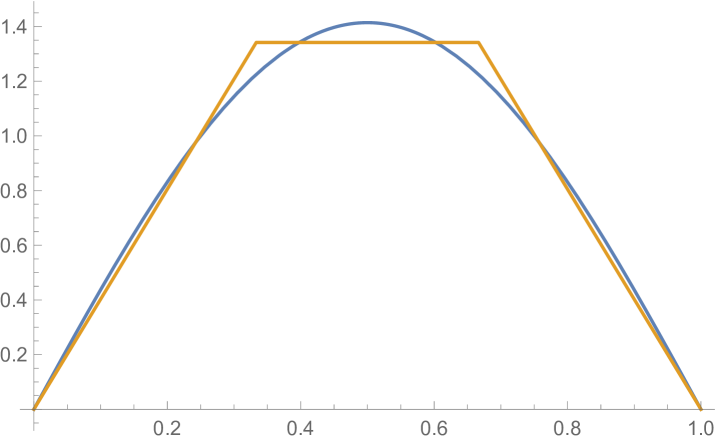
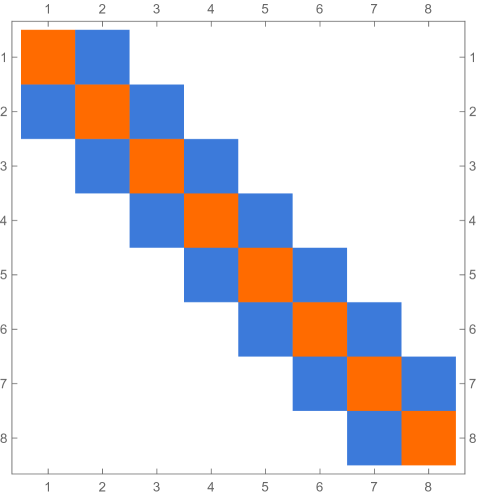
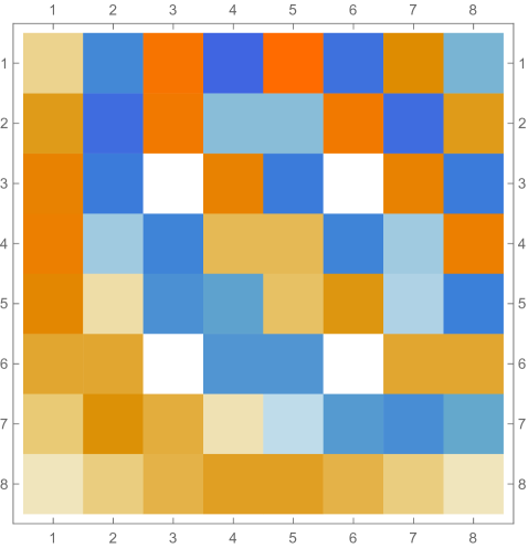
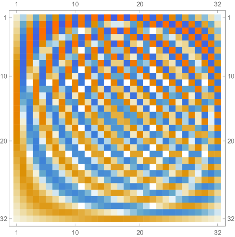
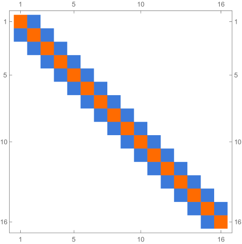
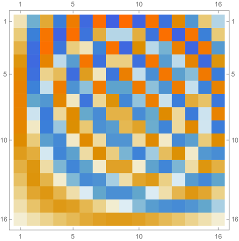
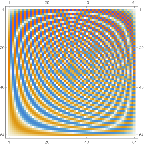
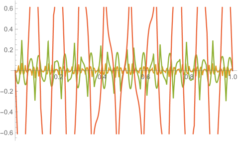
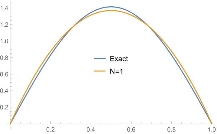
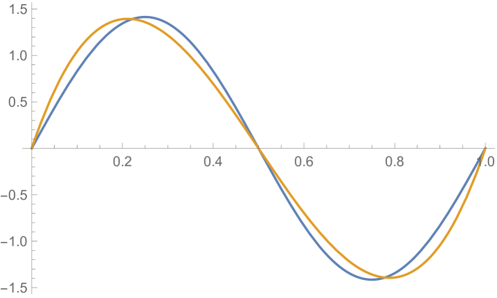
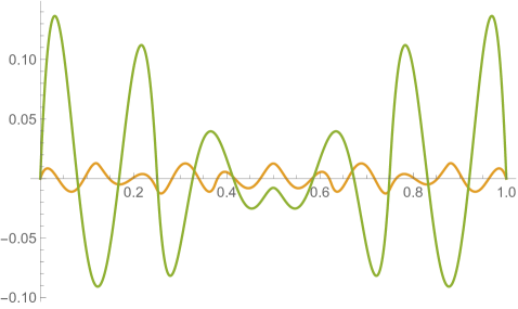
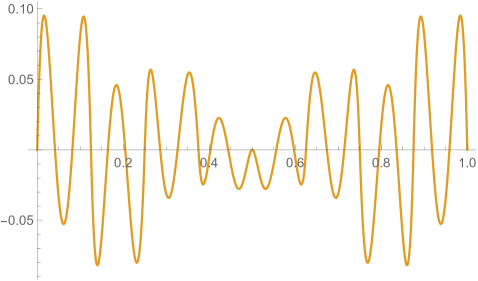
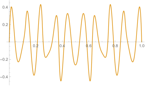
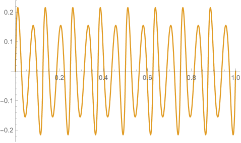
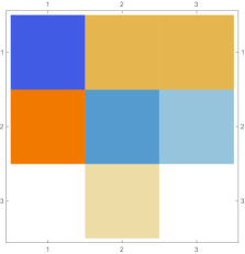
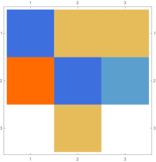
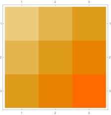
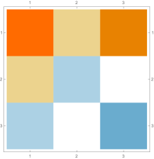
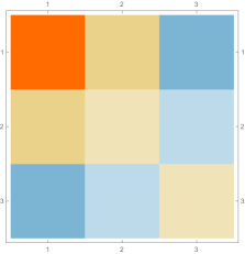
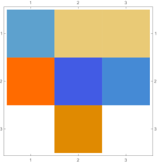
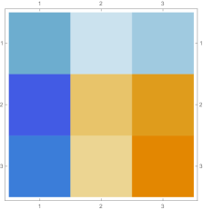
Fig. 4.1.1 compares simple discretization with and exact solution Eq. (4.1.2) for and . Note that these two wavefunctions are automatically orthogonal to each other. Fig. 4.1.2 shows two matrices ( and ) and normalized but not necessarily orthogonal eigenvectors produced by , , , and versions of simple discretization; the other two matrices ( and ) are omitted as the tridiagonal structure is the same. With increasing (note that has zero points between the two end points), the eigenvectors become less and less smooth.
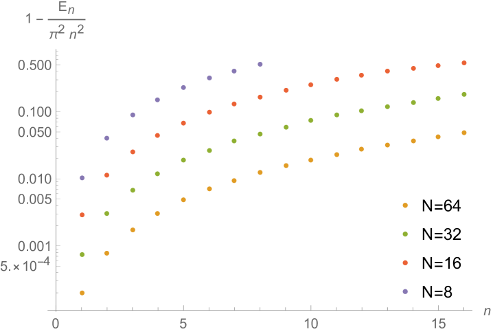
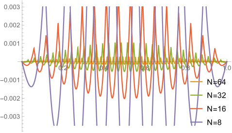
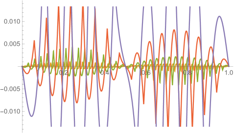
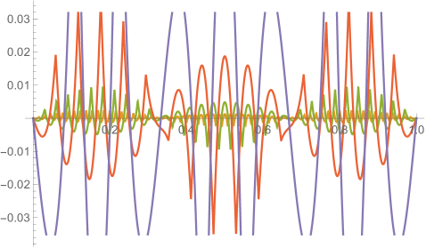
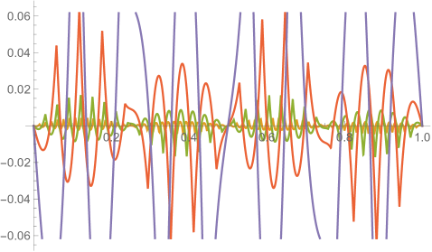
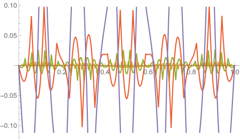
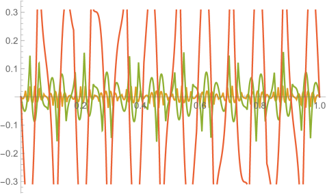
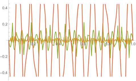
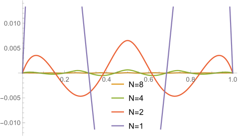
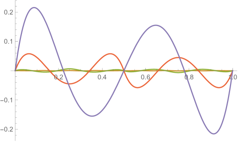
Figs. 4.1.3 and 4.1.4 display errors in eigenvalues and rendered eigenvectors of , , , and Hamiltonians, respectively. Although a Hermitian matrix has eigenpairs, and with are not shown in these figures. At small , the approximated wavefunctions are reasonably smooth; however, as approaches , the broken features become much more noticeable. It should be noted that all the eigenvalues produced by simple discretization are smaller than their exact counterparts, unlike those yielded by first ContEvol method, as we will show in the next section.
4.2 Infinite potential well, first-order ContEvol
Now we present the ContEvol treatment of the same problem. We divide the interval into equal parts with nodes
| (4.2.1) |
investigating if an unequal partition leads to better results is left for future work. With and , the wavefunction is sampled as
| (4.2.2) |
with
| (4.2.3) |
where is the length of each sub-interval. Boundary conditions at and indicate that . The desired approximation is represented in the same way.
We are supposed to have . Note that and are both piecewise cubic functions with continuous first derivatives, while is a piecewise linear function which is not necessarily continuous at sampling nodes. The cost function is defined as (subscript “IPW” stands for infinite potential well)
| (4.2.4) |
for simplicity, in the following text we omit parameters of , which is
| (4.2.5) |
for ; plugging in expressions of , , , and , this becomes
| (4.2.6) |
for convenience, we define .
Partial derivatives of with respect to , , , and are
| (4.2.7) |
respectively; note that one should not set these to zero, as a node is coupled with two adjacent intervals, unless it is or . Put in matrix form, these are
| (4.2.8) |
again for convenience, we define .
To minimize the cost function Eq. (4.2.4), we have
| (4.2.9) |
since
| (4.2.10) |
the and matrices can be constructed from scratch (zero matrix) by doing
| (4.2.11) |
where denotes the addition assignment operator in common programming languages like C or Python, for . To enforce the constraints, one simply needs to remove the corresponding rows and columns.
Our desired Hamiltonian is thus simply . Eigendecomposition of should yield (or ) eigenpairs, and , without (with) those two constraints. With or without the enforcement, and matrices are always symmetric; however, this does not guarantee that the resulting matrix is also symmetric, and thus Hermitian.
Like in Section 4.1, the eigenvectors need to be “renormalized” as
| (4.2.12) |
they may need to be “reorthogonalized” according to the “inner product” defined as follows
| (4.2.13) |
Toy version: .
While and , with enforced, the and matrices are simply
| (4.2.14) |
and the Harmiltonian is
| (4.2.15) |
Realistic versions: , , and .
Although the toy version results seem promising, one needs to use a larger for more accurate results and larger quantum numbers.
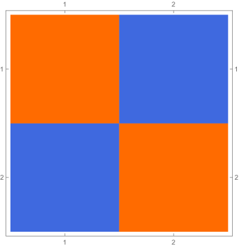
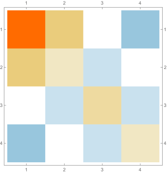
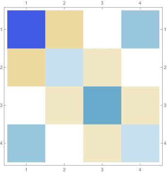
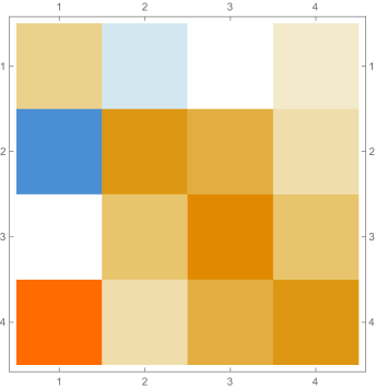
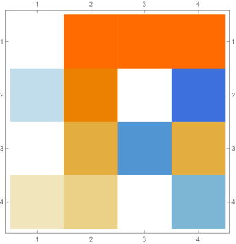
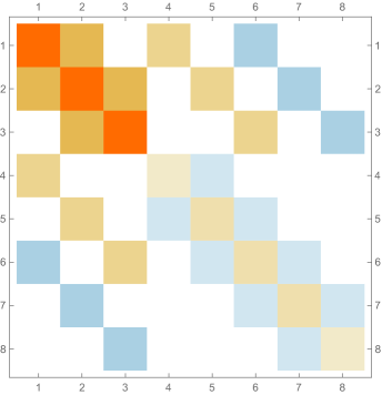
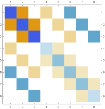
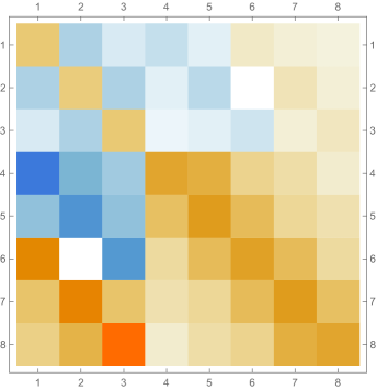
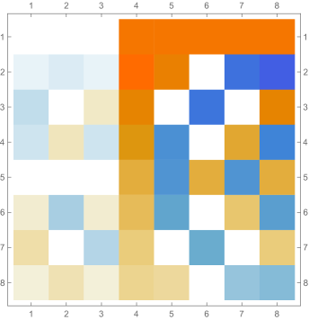
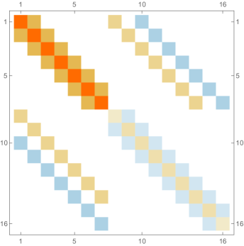
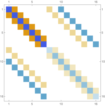
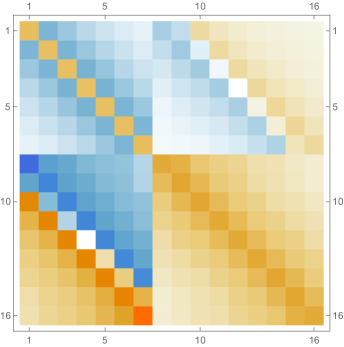
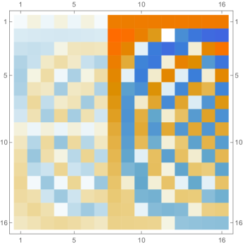
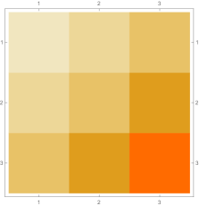
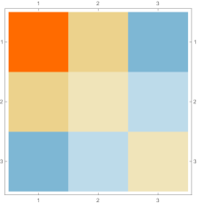
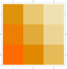
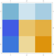
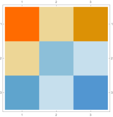
Fig. 4.2.2 shows , , and matrices, as well as normalized but not necessarily orthogonal eigenvectors produced by , , , and versions of first-order ContEvol. , , and are all matrices. In each of them, the upper left blocks (absent in the case) describes coupling between and , the lower right blocks describes coupling between and , and they other two blocks (both absent in the case) describe coupling between values and derivatives. All these blocks are tridiagonal; because of the special form of and submatrices Eq. (4.2), the central diagonals of the cross blocks are uniformly zero. From the third column, it is clear that the Hamiltonians are not symmetric; nevertheless, the upper left blocks (absent in the case) and the lower right blocks are symmetric. Intuitively, the Hamiltonians should still be Hermitian if we consider them as operators on function representations . Shown in the last column are the eigenvectors: the first components of each row (absent in the case) are for , while the last components are for . Similar patterns can be seen from eigenvectors with different values. For example, both and are zero or almost zero at nodes (not shown in the case), but the former has the same first derivatives, while the latter has alternating first derivatives.
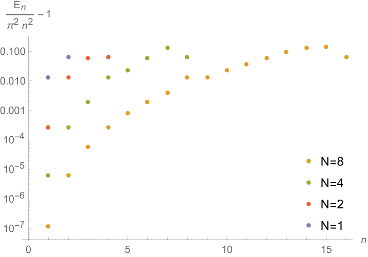
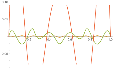
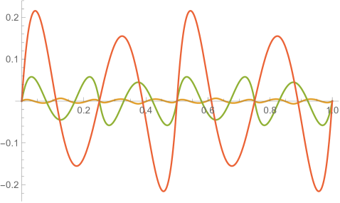
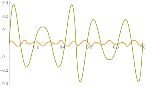
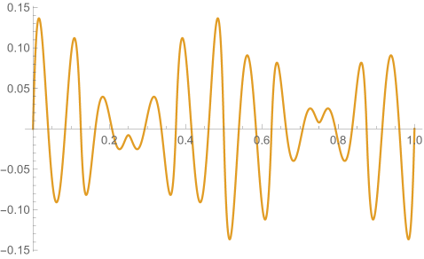
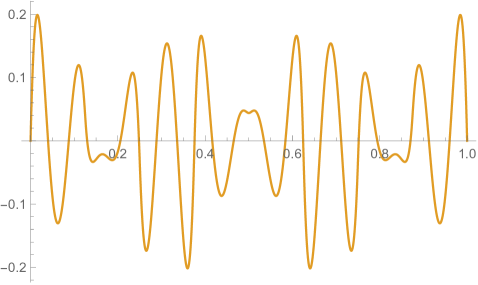
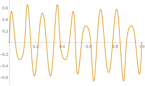
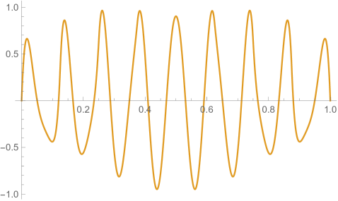
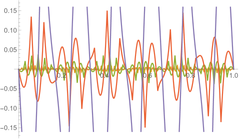
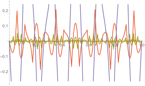
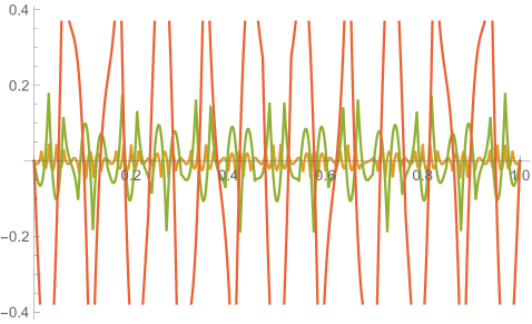
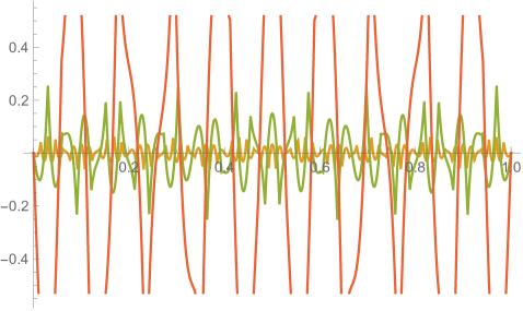
Figs. 4.2.3 and 4.2.4 display errors in eigenvalues and rendered eigenvectors of , , , and Hamiltonians, respectively. With only a quarter of the number of parameters used in simple discretization (see Section 4.1), ContEvol results are arguably better, especially for the ground state energy . Since a matrix only has (at most) eigenpairs, and with large are only available with large . The quality of the results significantly deteriorates as approaches ; it reaches the worst case at , and becomes reasonably good at , when our sampling nodes coincide with zero points of the wavefunctions. Based on these two figures, a rule of thumb would be to only trust results, so that errors in eigenvalues are below or at the level.
4.3 Harmonic oscillator, first-order ContEvol (description)
In this section, we consider (quantum) harmonic oscillator with potential
| (4.3.1) |
where we have set the constant to ; note that this only affects the scaling of . The exact wavefunctions can be expressed using Hermite polynomials; we do not include them here as no comparisons will be made.
As for application of the ContEvol method, there are three major differences between harmonic oscillator and infinite potential well, which we describe one by one.
Difference 1: Position-dependent potential.
In the case of infinite potential well, the potential is uniformly zero in the interval of interest; the case of harmonic oscillator is different. Consequently, each piece of the cost function needs to be written as (subscript “QHO” stands for quantum harmonic oscillator)
| (4.3.2) |
where we have omitted results of the expansion, squaring, integral, and substitution steps (“”). It should be noted that, fortunately, ContEvol is robust against complications induced by the position-dependent potential function, because is still a finite polynomial of , of which all coefficients are linear combinations of , , and .
In general, a potential function can be represented as and , even if it is a hard-to-integrate transcendental function or does not have an analytic form. In the regime of first-order ContEvol, each piece of possesses up to the third order in , ergo the resulting expression of each piece of the cost function has up to the thirteenth order in ; when is small, it is reasonable to truncate the expansion of the square root of the integrand at the third order in , so that the final expression has up to the seventh order in , like in Sections 2.1 or 3.1. Note that when denotes the length of each sub-interval, it is not necessarily small, specifically not necessarily smaller than , hence higher-order terms may be more important than lower-order ones.
Difference 2: Lack of sharp edges.
Unlike Eq. (4.1.1), Eq. (4.3.1) does not require wavefunctions to vanish at specific, finitely distant positions; figuratively speaking, wavefunctions are allowed to (and actually should) have tails. Therefore, we need to define and — not just for convenience, but also for accuracy.
Wavefunctions are supposed to vanish at infinity, i.e., satisfy and . Given and or and , it is impossible to find a cubic representation of in the interval or ; however, assuming that and have same signs while and have opposite signs, there is always a pair of exponential tails
| (4.3.3) |
satisfying all these boundary conditions. Expressing tails of in the same way, tails of the cost function could be defined as
| (4.3.4) |
where integrals of exponential tails multiplied by (actually polynomial potential functions in general) can be expressed using gamma function. Yet unfortunately, with and , and as denominators, such tails break the linearity of our ContEvol formalism. A natural solution would be to treat and , and as fixed values in the tails; as a price, one would need to fine-tune and , so that these ratios are indeed close to the corresponding fixed values. A related example will be presented in the next section.
As for second-order ContEvol, the tails could be similarly written as
| (4.3.5) |
however, even one is willing to deal with non-linearity, since the error function does not have an analytic form, one may need to build numerical lookup tables for and . In the linear regime, we can treat ratios like and to zeros as well, but it is not common for first and second derivatives to simultaneously satisfy constraints, hence we can only aim for having sensible and values. Better and possibly intricate circumvention is beyond the scope of this work.
Difference 3: Increasing “sizes” of wavefunctions.
For scenarios like (quantum) harmonic oscillator, the “sizes” of wavefunctions (which can be strictly quantified using percentiles of the probability distribution) increase with larger quantum numbers. Meanwhile, with nodes, first-order ContEvol is supposed to yield eigenvectors. Therefore, for similar problems, the spread of nodes probably needs to be adjusted according to test results. Since the fine-tuning may require several iterations, objective evaluation criteria can be designed to automate this process; such efforts are left for future work, and probably for specific situations.
To summarize, harmonic oscillator manifests some of the difficulties encountered in real-world problems, but ContEvol methods should be able to handle them reasonably well.
4.4 Coulomb potential, first-order ContEvol
In this final section on quantum mechanics, we look at a more realistic case, one-dimensional Coulomb potential. Following Section 2.1 of Pradhan and Nahar (2011), the radial part of the stationary Schrödinger equation for a hydrogen atom can be written as
| (4.4.1) |
where we have used atomic units, the potential , is the angular quantum number, and is a modified version of the radial wavefunction . This work focuses on the ground state , hence we set ; in our notation, the equation becomes
| (4.4.2) |
and the exact solution is
| (4.4.3) |
For simplicity, we sample the non-negative half of the real axis with nodes
| (4.4.4) |
where is the width of each interval101010Caution: In this section, is always a non-negative integer and never the imaginary unit.; non-uniform sampling is left for future work. To handle the factor in the equation, we require each piece of the wavefunction to be proportional to ; note that this strategy can be applied to Yukawa potential as well. Therefore the wavefunction is written as
| (4.4.5) |
where we exclude from the tail to maintain linearity of our framework.
The coefficients through are yielded by terminal conditions at and
| (4.4.6) |
since and , for we have
| (4.4.7) | ||||
| (4.4.8) |
Like in Section 4.2, the desired approximation is represented in the same way with and . For convenience, we put this linear transformation in matrix form
| (4.4.9) |
with the transformation matrix
| (4.4.10) |
which is the same for and . Boundary condition at indicates that . In the special case of , we set to get
| (4.4.11) |
or
| (4.4.12) |
so that .
The cost function is defined as (subscript “H” stands for hydrogen atom)
| (4.4.13) |
for simplicity, in the following text we omit parameters of , which is
| (4.4.14) |
where , for ; will be addressed later. Again for convenience, we define .
Partial derivatives of with respect to , , , and are
| (4.4.15) |
respectively; put in matrix form, these are
| (4.4.16) |
with
| (4.4.17) |
For the special case of , we simply need to drop the first rows and first columns of and . Then partial derivatives of with respect to , , , and can be succinctly expressed as
| (4.4.18) |
As promised, we now address , which corresponds to the tail. Given our assumed functional form Eq. (4.4.5), this should be
| (4.4.19) |
and its partial derivative with respect to is
| (4.4.20) |
where and are both matrices.
To minimize the cost function Eq. (4.4.13), we have
| (4.4.21) |
since
| (4.4.22) |
the and matrices can be constructed from scratch (zero matrix) by doing
| (4.4.23) |
for , and then
| (4.4.24) |
for , and finally
| (4.4.25) |
for .
Because of our definition of the tail, we need to enforce the constraint if we want to maintain the continuity of first derivative at . In this case, simply removing the corresponding rows and columns from and matrices constructed above would lead to erroneous results, as when four coefficients (, , , and ; similar for ) are fully specified by three parameters (, , and ; similar for ), the inverse transformation may not be well defined — the situation is basically the same as in Section 2.3.
Therefore, when and , we have to plug the two sets of three parameters into Eq. (4.4) to obtain (here the prime “′” denotes with the constraints mentioned above)
| (4.4.26) |
with
| (4.4.27) |
and
| (4.4.28) |
Note that although only the version of the above expressions is used in this work, we have written the general version for .
To construct the and matrices from scratch, the procedure is the same as when we do not enforce and , except for the st step, which needs to be substituted by
| (4.4.29) |
Our desired Hamiltonian is thus simply . Eigendecomposition of should yield (or ) eigenpairs, and , without (with) the constraint. With or without the enforcement, () matrices are always (never) symmetric; consequently, () matrices are also always (never) symmetric.
Like in Sections 4.1 and 4.2, the eigenvectors need to be “renormalized” as
| (4.4.30) |
we omit the “inner product” definition here as this section focuses on the ground state.
Special version: .
Because of the tail, it is possible to study the case, for which our wavefunction is simply
| (4.4.31) |
which, after normalization, coincides with the exact solution Eq. (4.4.3). Nevertheless, we still need to study the energy predicted by ContEvol.
In this special case, the cost function is
| (4.4.32) |
Evidently, minimizing this would yield , i.e., the Hamiltonian , and the ground state energy also coincides with the exact solution. Of course, such coincidence should not be relied upon, hence we move on to more realistic values.
Toy version: .
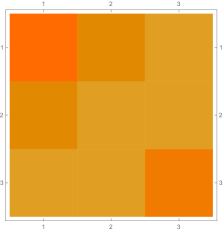
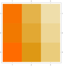

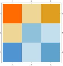
Then we explore the case, which only has one single interval in addition to the tail. Fig. 4.4.1 presents five sets of six matrices based on different values of . All non-zero elements of matrices are shown in gradually varying colors, illustrating how changes with ; note that Eq. (4.4.12) tells us that the matrix element is always regardless of . The symmetric matrices (with first rows and first columns dropped) manifest similar gradual variation, with largest element “migrating” from lower-right corner to upper-left corner; however, combining variations of and , as well as added for the tail, the matrices seem very similar to each other, although the color scales (not shown in Fig. 4.4.1) are different. The matrices (also with first rows and first columns dropped) are intrinsically asymmetric, and the largest element “migrates” from lower-center to lower-left; the resulting matrices seem quite different with different values of , yet gradual variation can still be revealed if we examine the elements one at a time. Finally, the matrices also look similar to each other, although slightly variation can still be noticed; their eigenvectors are not shown as a matrix, since this section focuses on the ground state. Here we comment that the other two eigenvalues are positive, and the corresponding wavefunctions are quasi-sinusoidal in the interval and almost zero in the tail; to study the actual excited states, one needs to repeat the fine-tuning exercise described below.
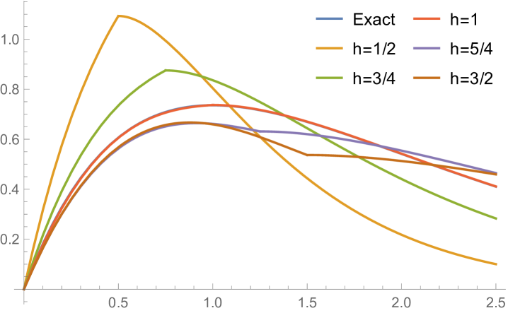
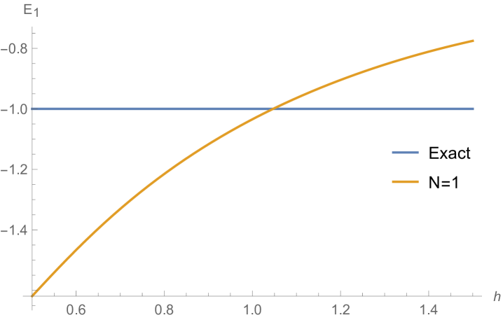
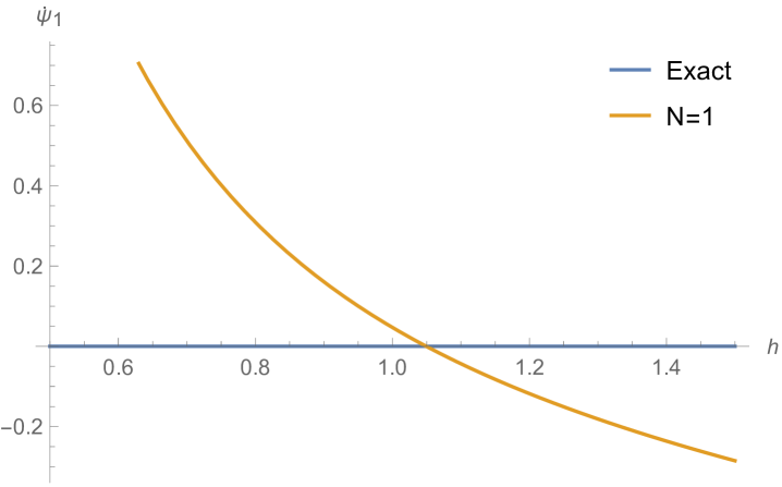
Rendered ground state wavefunctions based on the matrices in Fig. 4.4.1 are shown in the left panel of Fig. 4.4.2. The version agrees with the exact solution Eq. (4.4.3) remarkably well, while other values of are limited by not-so-good predefined functional forms. The right panel of Fig. 4.4.2 plots the ground state energy as a function of . The ContEvol solution coincides with the exact value at . However, how shall we determine the optimal value of when we have no idea about the exact solution? Similar to an argument in Section 4.3, we can fine-tune so that , in this case , is close to zero. Fig. 4.4.3 plots as a function of . It is exactly zero at , which is close but not identical to the value quoted above. In practice, we can adjust values of and in turn: for example, we explore a small interval around with , get a better estimate of , and explore a smaller interval around the updated with a larger , etc., until the errors are below some threshold. Such iterative process is not implemented for this work. In the following, we simply adopt , and enforce the constraint; investigating how affects the accuracy of results is left for future work.
Realistic versions: to .
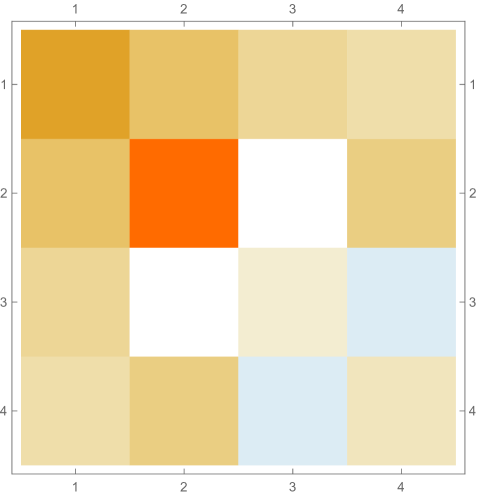
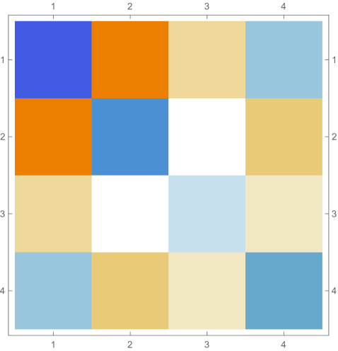
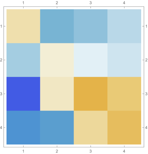
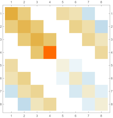
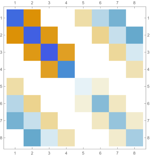
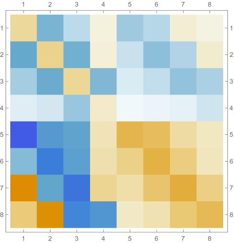
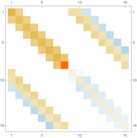
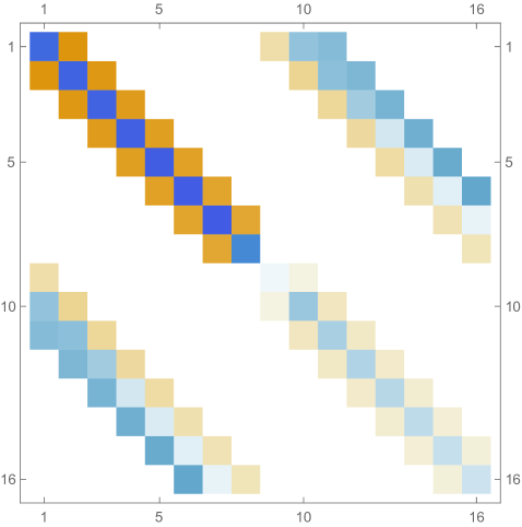
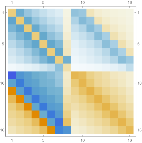
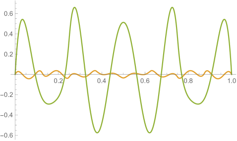
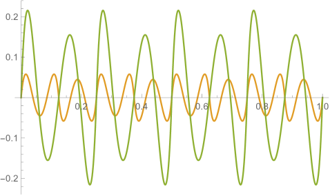
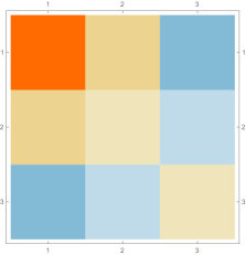
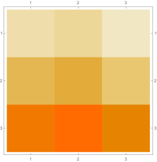
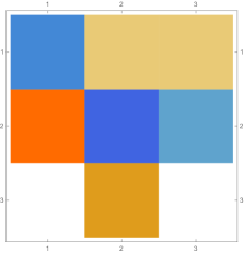
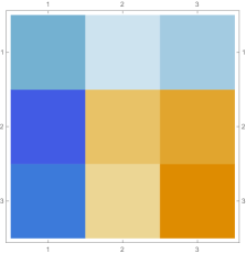
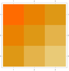
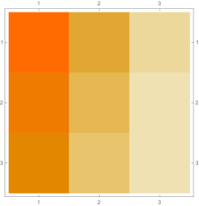
Fig. 4.4.4 shows , , and matrices produced by , , and versions of first-order ContEvol. Like in the case of infinite potential well (see Section 4.2, especially Fig. 4.2.2), each or matrix has tridiagonal blocks; because of the position-dependence of the Coulomb potential, elements on the same diagonal do not necessarily have the same value. Most noticeable matrix elements are and , which are affected by the tail; the former are “more positive” in matrices, while the latter are “less negative” in matrices. Consequently, the th rows and th columns of matrices do not follow the same pattern as other regions.
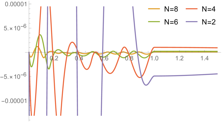
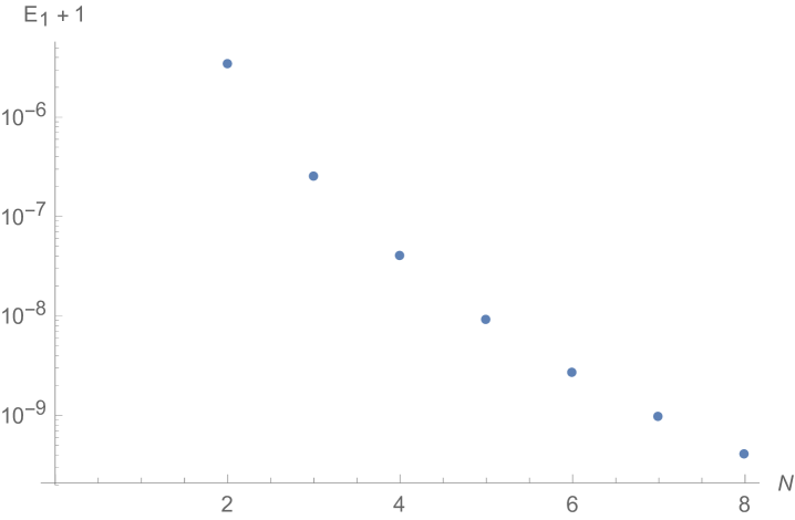
In Fig. 4.4.5, the left panel displays errors in rendered ground state wavefunctions of , , (not shown in Fig. 4.4.4), and Hamiltonians, while the right panel plots errors in ground state energy predicted by first-order ContEvol with . Like in Section 4.2, the eigenpair is already remarkably accurate with , which is arguably small.
5 Discussion: directions for future work
The ContEvol formalism has many potential applications inside and outside physics. For example, yearn for a “smoother” stellar evolution code has supplied the original motivation for this work. As long as people want to represent continuous functions (of time, space, or both) with a finite sampling, ContEvol may help. However, much work remains to be done to reveal its full potential. In this final section, we discuss some of the major directions for future development of ContEvol.
Mathematical foundation.
Although ContEvol appears to be successful, it lacks a solid mathematical foundation. Desirable justifications and auxiliary tools include but are not limited to:
-
•
Control over errors and non-symplecticity. With specific cases, this work seems to indicate that first-order ContEvol results have errors in values, errors in first derivatives, and error in deviation from equation(s) of motion — more specifically, the terms in values are usually just missing, see Eq. (2.1.12) for an example; second-order ContEvol does not improve order of errors in results, but does reduce deviation from EOM(s) to ; non-symplecticity (discrepancy between determinant of Jacobian and ) does not display a uniform pattern. Under what conditions do these statements hold? How do these quotes scale with the order of ContEvol? Such questions needs to be answered to solidify ContEvol results.
-
•
Foundation for customized Linear algebra. As hypothesized in Section 4.2, intuitively Hamiltonian based on Eq. (4.2.9) should be a Hermitian operator, and inner product defined in Eq. (4.2) is reasonable. Yet unless these statements are well justified, ContEvol does not guarantee an expected number of valid eigenpairs.
-
•
Moments and transforms. This work has not included expressions for moments and transforms (e.g., Fourier and Laplace transforms) based on values and derivatives at nodes, yet such things are likely to be important for the analysis of ContEvol results. Do they reveal additional properties or limitations of ContEvol methods? The answer will inform choices for specific applications.
Higher dimensions.
This work has been focused on one-dimensional scenarios, either time or space; nevertheless, the combination of function representation with linear coefficients and cost function minimization can be generalized to high-dimensional cases. In other words, the ContEvol formalism should be able to solve partial differential equations (PDEs) as well as ordinary differential equations (ODEs). Here we outline major directions of such extensions for first-order ContEvol.
-
•
Evolving one-dimensional functions. In this case, the full evolutionary history of the function , sampled at timestamps and nodes, can be fully characterized by quadruples, , where semicolons “;” in subscripts denote partial derivatives. Thus at each space-time location, the function can be rendered as the product of a cubic polynomial in and a cubic polynomial in ; such a representation has coefficients, corresponding to four quadruples at four corners of a space-time cell.
-
•
Representing high-dimensional functions. Although there are no restrictions for use of curvilinear coordinates, the discussion here focuses on Cartesian coordinates. To fully characterize a spatial distribution, in principle one could use in two dimensions and in three dimensions. However, in dimensions, multiplying the growth of number of nodes and growth of number of features can easily make things computationally unaffordable. A less expensive version of the high-dimensional function representation would only use values and first derivatives, i.e., in 2D and in 3D, so that the number of features only grows as . A difficulty is that in 2D (3D), there are only (or ) zeroth- to third-order terms, but there are (or ) features to fit for each cell; to bypass inconsistency, it is recommended to add some higher-order terms (e.g., ), but those involving fourth or higher order in a single variable should probably be avoided (e.g., or ).
-
•
Evolving high-dimensional functions. Space and time coordinates could be viewed as equivalent from the perspective of special relativity, yet for most computational physics problems, time may play a different role than spatial coordinates. Thenceforth, for better representing the “history” of a dynamic system, in 2D and in 3D might be a more sensible choice.
In addition to higher dimensions, we note that extension to multiple functions is also natural; vector and tensor functions can be decomposed into independent components, as we did in Section 3.
Technical improvements.
The last group of directions addresses some technical issues involved in the ContEvol formalism per se, which may lead to improvements in accuracy, precision, or performance.
-
•
Multistep version. This works has been focused on single-step ContEvol methods, regardless of the order, yet it is possible to extend ContEvol to multiple steps or intervals. For boundary value problems, if we want to study the function for some interval , while the combination of can give us a cubic approximation, the combination of (assuming sampling nodes and both exist or can be reasonably defined for convenience) can give us a septic approximation. For initial value problems, there are two basic strategies: backward, which for example approximates the evolution during the next interval as a quintic polynomial based on ; and forward, which for example approximates the evolution during the next two intervals as a pair of cubic polynomials or a unified quintic polynomial based on . Of course one can include more steps or devise hybrid versions. Like higher orders (e.g., Section 2.3), inclusion of multiple steps complicates derivation and computation, but potentially improves accuracy or precision.
-
•
Better sampling and evolving nodes. As mentioned in Section 4.2, the distribution of sampling nodes is by no means necessarily uniform; for some realistic applications, their distribution should not be fixed, for example in Section 4.3, when the potential function necessitates a flexible sampling. In short, the sampling is something ContEvol users are encouraged to fine-tune. In addition, when a field is evolved (see above for discussion on higher dimensions), drifting nodes (i.e., nodes with varying positions) and splitting or merging cells (i.e., adding or removing nodes) may be desirable. Because of the uniqueness of Hermite spline, splitting into and by inserting and at an arbitrary location between and does not distort the “current” function representation at all; this fact should be applicable to higher dimensions as well. However, we note that such variations are preferably predefined (e.g., according to some strategy), not determined on-the-fly, as optimizing location of nodes often requires solving non-linear equations.
-
•
Computational efficiency. Let us consider arguably the most costly case of real-world physics problems, time evolution of a set of three-dimensional fields, e.g., cosmological simulations; we use single-step ContEvol with nodes in each dimension, and keep track of quantities, each with features (i.e., values or partial derivatives). Then the dimension of the matrix is , which can be overwhelmingly expensive. However, indexing each of the blocks as , where , the necessary condition for an element to be non-zero is . In other words, among the elements of this block, only less than can possibly non-zero, i.e., such matrices are highly sparse when is large; a closer look would reveal many “tridiagonal” structures. Specialized data structures and algorithms could be designed to handle such matrices. Furthermore, when we compute the evolution of large-scale structures under gravitational interactions, information about specific chemical composition may not be particularly pertinent. In such cases, multi-tier strategy could be useful: at each step, we first evolve the “dominating” quantities, and then combine coarse-grained “future” and fine-grained “present” to evolve the “dependent” quantities.
Miscellany.
In addition to the above directions, some miscellaneous topics are worth mentioning.
-
•
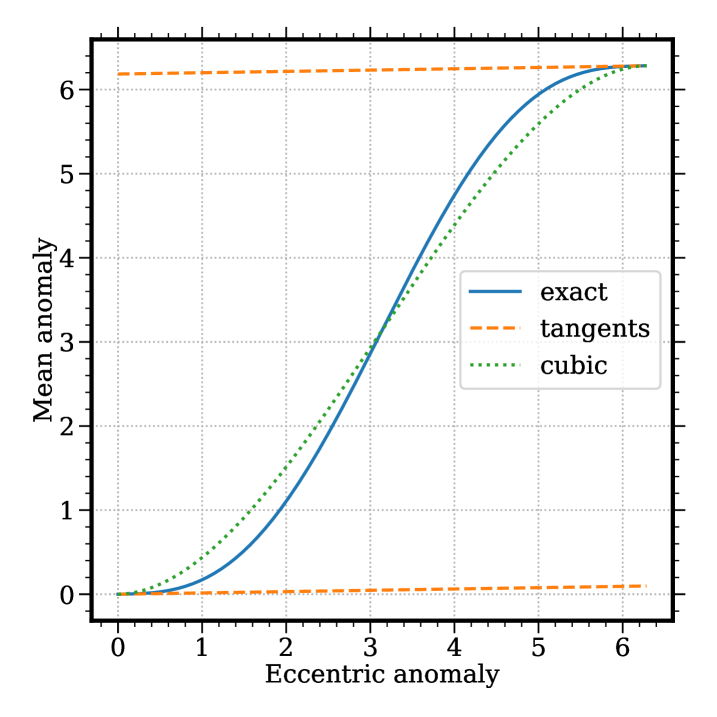
Root-finding. While this work has been focused on differential equations, the backbone function representation of ContEvol (Hermite spline) can be applied to algebraic equations as well: knowing both values and first derivatives at two sampling points, we can always find a cubic approximation of the function to help root-finding. For instance, Fig. 5.0.1 displays Kepler’s equation Eq. (3.4.8) with ; using Newton’s method, one would have to carefully choose an initial guess to avoid divergence, while the cubic approximation is more robust. Admittedly, solution to a cubic equation is more complicated than that to a linear equation, yet cubic may work better in some cases; besides, one can use cubic for the first few steps, and then switch to linear for fine-tuning purposes.
-
•
Numerical integration. Likewise, piece-wise cubic (or higher-order) polynomials may help numerical integration. As demonstrated in Section 4, using less sampling points, a “compound” sampling with both values and derivatives can outperform “simple” sampling with only values. Although fitting polynomials with multiple values (e.g., Simpson’s rule) could effectively mitigate discreteness, usage of derivatives should rely less on a fine sampling. When the derivatives have to be evaluated numerically, in the first-order case, this technical is equivalent to a sampling like , where .
-
•
Data structure of lookup tables. Due to the semi-analytic nature of the ContEvol formalism, its performance might be limited by lookup tables stored as hypercubes of values; fortunately, development of numerical methods may advance data structure of lookup tables as well. This section has already addressed how high-dimensional functions are supposed to be digitalized by combining values and derivatives; the three-dimensional plan can be naturally extended to higher dimensions. Even without ContEvol, “continuous” lookup tables have their own benefits, e.g., higher accuracy or less storage usage.
In conclusion, it is our hope that, with further developments, the ContEvol (continuous evolution) formalism can benefit some applications of computational physics.
Acknowledgements and data availability
KC thanks his advisors, Christopher M. Hirata and Marc H. Pinsonneault, for inspirations through research projects in cosmological image processing and stellar evolution, respectively, as well as insights and encouragement during the preparation of this work. KC appreciates insightful feedback from (in chronological order) Anil K. Pradhan, Annika H.G. Peter, R.J. Furnstahl, and Todd A. Thompson. KC also thanks Li-Yong Zhou (周礼勇; Nanjing University, China) and R.J. Furnstahl for introducing him to numerical methods in celestial mechanics and quantum mechanics, respectively.
During the preparation of this article, KC is supported by an internal funding source at The Ohio State University. The following software is used on KC’s personal computer (HP All-in-One 24-dp1xxx, Microsoft Windows 11 Home). Most symbolic operations throughout this work are performed and figures in Section 4 are made with Wolfram Mathematica 11.0 (Inc., ). Numerical tests in Section 3 are conducted with Python 3.11 (van Rossum and Team, 2023) codes developed using NumPy (Harris et al., 2020) and Numba (Lam et al., 2015), corresponding exact solution is derived with SciPy (Virtanen et al., 2020), while figures therein and that in Section 5 are made with Matplotlib (Hunter, 2007). Mathematica and Jupyter notebooks for this work will be available in the GitHub repository ContEvol_formalism111111https://github.com/kailicao/ContEvol_formalism.git after it is posted on arXiv. This article is prepared with Overleaf, Online LaTeX Editor121212https://www.overleaf.com/ and Online LaTeX Equation Editor131313https://latex.codecogs.com/eqneditor/editor.php.
References
- Springel [2010] Volker Springel. E pur si muove: Galilean-invariant cosmological hydrodynamical simulations on a moving mesh. MNRAS, 401(2):791–851, January 2010. 10.1111/j.1365-2966.2009.15715.x.
- Jiang et al. [2014] Yan-Fei Jiang, James M. Stone, and Shane W. Davis. An Algorithm for Radiation Magnetohydrodynamics Based on Solving the Time-dependent Transfer Equation. ApJS, 213(1):7, July 2014. 10.1088/0067-0049/213/1/7.
- Bovy [2015] Jo Bovy. galpy: A python Library for Galactic Dynamics. ApJS, 216(2):29, February 2015. 10.1088/0067-0049/216/2/29.
- Demarque et al. [2008] P. Demarque, D. B. Guenther, L. H. Li, A. Mazumdar, and C. W. Straka. YREC: the Yale rotating stellar evolution code. Non-rotating version, seismology applications. Ap&SS, 316(1-4):31–41, August 2008. 10.1007/s10509-007-9698-y.
- Paxton et al. [2011] Bill Paxton, Lars Bildsten, Aaron Dotter, Falk Herwig, Pierre Lesaffre, and Frank Timmes. Modules for Experiments in Stellar Astrophysics (MESA). ApJS, 192(1):3, January 2011. 10.1088/0067-0049/192/1/3.
- Chambers [1999] J. E. Chambers. A hybrid symplectic integrator that permits close encounters between massive bodies. MNRAS, 304(4):793–799, April 1999. 10.1046/j.1365-8711.1999.02379.x.
- Rein and Liu [2012] H. Rein and S. F. Liu. REBOUND: an open-source multi-purpose N-body code for collisional dynamics. A&A, 537:A128, January 2012. 10.1051/0004-6361/201118085.
- Grandclément and Novak [2009] Philippe Grandclément and Jérôme Novak. Spectral Methods for Numerical Relativity. Living Reviews in Relativity, 12(1):1, January 2009. 10.12942/lrr-2009-1.
- Press et al. [2007] W.H. Press, S.A. Teukolsky, W.T. Vetterling, and B.P. Flannery. Numerical Recipes: The Art of Scientific Computing. Cambridge University Press, 3 edition, 2007. ISBN 9780521880688. URL http://nr.com/.
- Pradhan and Nahar [2011] Anil K. Pradhan and Sultana N. Nahar. Atomic Astrophysics and Spectroscopy. Cambridge University Press, 2011.
- [11] Wolfram Research, Inc. Mathematica, Version 11.0. Champaign, IL, 2016.
- van Rossum and Team [2023] G. van Rossum and Python Development Team. Python Language Reference Release 3. 11. 3. Lulu Press, Incorporated, 2023. ISBN 9781312573949. URL https://books.google.com/books?id=QiTwzwEACAAJ.
- Harris et al. [2020] Charles R. Harris, K. Jarrod Millman, Stéfan J. van der Walt, Ralf Gommers, Pauli Virtanen, David Cournapeau, Eric Wieser, Julian Taylor, Sebastian Berg, Nathaniel J. Smith, Robert Kern, Matti Picus, Stephan Hoyer, Marten H. van Kerkwijk, Matthew Brett, Allan Haldane, Jaime Fernández del Río, Mark Wiebe, Pearu Peterson, Pierre Gérard-Marchant, Kevin Sheppard, Tyler Reddy, Warren Weckesser, Hameer Abbasi, Christoph Gohlke, and Travis E. Oliphant. Array programming with NumPy. Nature, 585(7825):357–362, September 2020. 10.1038/s41586-020-2649-2.
- Lam et al. [2015] Siu Kwan Lam, Antoine Pitrou, and Stanley Seibert. Numba: A LLVM-based Python JIT Compiler. In Proc. Second Workshop on the LLVM Compiler Infrastructure in HPC, pages 1–6, November 2015. 10.1145/2833157.2833162.
- Virtanen et al. [2020] Pauli Virtanen, Ralf Gommers, Travis E. Oliphant, Matt Haberland, Tyler Reddy, David Cournapeau, Evgeni Burovski, Pearu Peterson, Warren Weckesser, Jonathan Bright, Stéfan J. van der Walt, Matthew Brett, Joshua Wilson, K. Jarrod Millman, Nikolay Mayorov, Andrew R. J. Nelson, Eric Jones, Robert Kern, Eric Larson, C. J. Carey, İlhan Polat, Yu Feng, Eric W. Moore, Jake VanderPlas, Denis Laxalde, Josef Perktold, Robert Cimrman, Ian Henriksen, E. A. Quintero, Charles R. Harris, Anne M. Archibald, Antônio H. Ribeiro, Fabian Pedregosa, Paul van Mulbregt, and SciPy 1. 0 Contributors. SciPy 1.0: fundamental algorithms for scientific computing in Python. Nature Methods, 17:261–272, February 2020. 10.1038/s41592-019-0686-2.
- Hunter [2007] John D. Hunter. Matplotlib: A 2D Graphics Environment. Computing in Science and Engineering, 9(3):90–95, May 2007. 10.1109/MCSE.2007.55.