This paper was converted on www.awesomepapers.org from LaTeX by an anonymous user.
Want to know more? Visit the Converter page.

Contextual Bandits for Unbounded Context Distributions

Puning Zhao    Rongfei Fan    Shaowei Wang    Li Shen    Qixin Zhang    Zong Ke    Tianhang Zheng
Abstract

Nonparametric contextual bandit is an important model of sequential decision making problems. Under α\alpha-Tsybakov margin condition, existing research has established a regret bound of O~(T1α+1d+2)\tilde{O}\left(T^{1-\frac{\alpha+1}{d+2}}\right) for bounded supports. However, the optimal regret with unbounded contexts has not been analyzed. The challenge of solving contextual bandit problems with unbounded support is to achieve both exploration-exploitation tradeoff and bias-variance tradeoff simultaneously. In this paper, we solve the nonparametric contextual bandit problem with unbounded contexts. We propose two nearest neighbor methods combined with UCB exploration. The first method uses a fixed kk. Our analysis shows that this method achieves minimax optimal regret under a weak margin condition and relatively light-tailed context distributions. The second method uses adaptive kk. By a proper data-driven selection of kk, this method achieves an expected regret of O~(T1(α+1)βα+(d+2)β+T1β)\tilde{O}\left(T^{1-\frac{(\alpha+1)\beta}{\alpha+(d+2)\beta}}+T^{1-\beta}\right), in which β\beta is a parameter describing the tail strength. This bound matches the minimax lower bound up to logarithm factors, indicating that the second method is approximately optimal.

Machine Learning, ICML

1 Introduction

Multi-armed bandit (Robbins, 1952; Lai & Robbins, 1985) is an important sequential decision problem that has been extensively studied (Agrawal, 1995; Auer et al., 2002; Garivier & Cappé, 2011). In many practical applications such as recommender systems and information retrieval in healthcare and finance (Bouneffouf et al., 2020), decision problems are usually modeled as contextual bandits (Woodroofe, 1979), in which the reward depends on some side information, called contexts. At the tt-th iteration, the decision maker observes the context 𝐗t\mathbf{X}_{t}, and then pulls an arm At𝒜A_{t}\in\mathcal{A} based on 𝐗t\mathbf{X}_{t} and the previous trajectory (𝐗i,Ai),i=1,,t1(\mathbf{X}_{i},A_{i}),i=1,\ldots,t-1. Many research assume linear rewards (Abbasi-Yadkori et al., 2011; Bastani & Bayati, 2020; Bastani et al., 2021; Qian et al., 2023; Langford & Zhang, 2007; Dudik et al., 2011; Chu et al., 2011; Li et al., 2010), which is restrictive and may not fit well into practical scenarios. Consequently, in recent years, nonparametric contextual bandits have received significant attention, which does not make any parametric assumption about the reward functions (Perchet & Rigollet, 2013; Guan & Jiang, 2018; Gur et al., 2022; Blanchard et al., 2023; Suk & Kpotufe, 2023; Suk, 2024; Cai et al., 2024).

Despite significant progress on nonparametric contextual bandits, existing studies focus only on the case with bounded contexts, and the probability density functions (pdf) of the contexts are required to be bounded away from zero. However, many practical applications often involve unbounded contexts, such as healthcare (Durand et al., 2018), dynamic pricing (Misra et al., 2019) and recommender systems (Zhou et al., 2017). In particular, the contexts may follow a heavy-tailed distribution (Zangerle & Bauer, 2022), which is significantly different from bounded contexts. Therefore, to bridge the gap between theoretical studies and practical applications of contextual bandits, an in-depth theoretical study of unbounded contexts is crucially needed. Compared with bounded contexts, heavy-tailed context distribution requires the learning method to be adaptive to the pdf of contexts, in order to balance the bias and variance of the estimation of reward functions. On the other hand, compared with existing works on nonparametric classification and regression with identically and independently distributed (i.i.d) data, bandit problems require us to achieve a good balance between exploration and exploitation, thus the learning method needs to be adaptive to the suboptimality gap of reward functions. Therefore, the main challenge of solving nonparametric contextual bandit problems with unbounded contexts is to achieve both bias-variance tradeoff and exploration-exploitation tradeoff using a single algorithm.

Method Bound of expected regret
Bounded context Heavy-tailed context
(Rigollet & Zeevi, 2010) UCBogram O~(T1min{α+1d+2,2d+2})\tilde{O}\left(T^{1-\min\left\{\frac{\alpha+1}{d+2},\frac{2}{d+2}\right\}}\right) None
(Perchet & Rigollet, 2013) ABSE O~(T1α+1d+2)\tilde{O}\left(T^{1-\frac{\alpha+1}{d+2}}\right) None
(Gur et al., 2022) SACB O~(T1α+1d+2)\tilde{O}\left(T^{1-\frac{\alpha+1}{d+2}}\right) None
(Guan & Jiang, 2018) kNN-UCB O~(Td+1d+2)\tilde{O}\left(T^{\frac{d+1}{d+2}}\right) None
(Reeve et al., 2018) kNN-UCB O~(T1α+1d+2)\tilde{O}\left(T^{1-\frac{\alpha+1}{d+2}}\right) None
This work kNN-UCB111Despite that the name kNN-UCB is the same as (Guan & Jiang, 2018) and (Reeve et al., 2018), the calculations of UCB are different between these methods. See details in the ”Nearest neighbor method with fixed kk” section. O~(Tmax{1α+1d+2,2α+3})\tilde{O}\left(T^{\max\left\{1-\frac{\alpha+1}{d+2},\frac{2}{\alpha+3}\right\}}\right) O~(T1βmin(d,α+1)min(d1,α)+max(1,dβ)+2β)\tilde{O}\left(T^{1-\frac{\beta\min(d,\alpha+1)}{\min(d-1,\alpha)+\max(1,d\beta)+2\beta}}\right)
This work Adaptive kNN-UCB O~(T1α+1d+2)\tilde{O}\left(T^{1-\frac{\alpha+1}{d+2}}\right) O~(T1min{(α+1)βα+(d+2)β,β})\tilde{O}\left(T^{1-\min\left\{\frac{(\alpha+1)\beta}{\alpha+(d+2)\beta},\beta\right\}}\right)
Minimax lower bound Ω(T1α+1d+2)\Omega\left(T^{1-\frac{\alpha+1}{d+2}}\right) Ω(T1min{(α+1)βα+(d+2)β,β})\Omega\left(T^{1-\min\left\{\frac{(\alpha+1)\beta}{\alpha+(d+2)\beta},\beta\right\}}\right)
Table 1: Comparison of the TT-step expected cumulative regrets of learning algorithms for nonparametric contextual bandits with Lipschitz reward function under α\alpha-Tsybakov margin condition and tail parameter β\beta (Assumption 1(a) and (b)).

In this paper, we solve the nonparametric contextual bandit problem with heavy-tailed contexts. To begin with, we derive a minimax lower bound that characterizes the theoretical limits of contextual bandit learning. We then propose a relatively simple method that uses fixed kk combined with upper confidence bound (UCB) exploration and derive the bound of expected regret. Even for bounded contexts, our method improves over an existing nearest neighbor method (Guan & Jiang, 2018) for large margin parameter α\alpha, since our method uses an improved UCB calculation which is more adaptive to the suboptimality gap of reward functions. Despite such progress, there is still some gap between the regret bound and the minimax lower bound, indicating room for further improvement. To close such a gap, we further propose a new adaptive nearest neighbor approach, which selects kk adaptively based on the density of samples and the suboptimality gap of reward functions. Our analysis shows that the regret bound of this new method nearly matches the minimax lower bound up to logarithmic factors, indicating that this method is approximately minimax optimal.

The general guidelines of our adaptive kNN method are summarized as follows. Firstly, with higher context pdf, we use larger kk, and vice versa. Secondly, given a specific context, if the value of an action is far away from optimal (i.e. large suboptimality gap), then we use smaller kk, and vice versa. Such a choice of kk achieves a good tradeoff between estimation bias and variance. With a lower pdf or larger suboptimality gap, the samples are relatively more sparse. As a result, a large bias may happen due to large kNN distances. Therefore, we use smaller kk to control the bias. On the contrary, with a higher pdf or smaller suboptimality gap, the samples are dense and thus we can use larger kk to reduce the variance. Note that the pdf and the suboptimality gap are unknown to the learner. Therefore, we design a method, such that the value of kk is selected by a data-driven manner, based on the density of existing samples.

1.1 Contribution

The contributions of this paper are summarized as follows.

  • We derive the minimax lower bound of nonparametric contextual bandits with heavy-tailed context distributions.

  • We propose a simple kNN method with UCB exploration. The regret bound matches the minimax lower bound with small α\alpha and large β\beta.

  • We propose an adaptive kNN method, such that kk is selected based on previous steps. The regret bound matches the minimax lower bound under all parameter regimes.

Our results and the comparison with related works are summarized in Table 1. In general, to the best of our knowledge, our work is the first attempt to handle heavy-tailed context distribution in contextual bandit problems. In particular, our new proposed adaptive kNN method achieves the minimax lower bound for the first time. The proofs of all theoretical results in the paper are shown in the supplementary material.

2 Related Work

In this section, we briefly review the related works about contextual bandits and nearest neighbor methods.

Nonparametric contextual bandits with bounded contexts. (Yang & Zhu, 2002) first introduced the nonparametric contextual bandit problem, proposed an ϵ\epsilon-greedy approach and proved the consistency. (Rigollet & Zeevi, 2010) derived a minimax lower bound on the regret, and showed that this bound is achievable by a UCB method. (Perchet & Rigollet, 2013) proposed Adaptively Binned Successive Elimination (ABSE), which adapts to the unknown margin parameter. (Qian & Yang, 2016) proposed a kernel estimation method. (Hu et al., 2020) analyzed nonparametric bandit problem under general Hölder smoothness assumption. (Gur et al., 2022) proposed Smoothness-Adaptive Contextual Bandits (SACB), which is adaptive to the smoothness parameter. (Slivkins, 2014; Suk & Kpotufe, 2023; Akhavan et al., 2024; Ghosh et al., 2024; Komiyama et al., 2024; Suk, 2024) analyzed the problem of dynamic regret. Furthermore, (Wanigasekara & Yu, 2019; Locatelli & Carpentier, 2018; Krishnamurthy et al., 2020; Zhu et al., 2022) discussed the case with continuous actions.

Nearest neighbor methods. Nearest neighbor classification has been analyzed in (Chaudhuri & Dasgupta, 2014; Döring et al., 2018) for bounded support of features. (Gadat et al., 2016; Kpotufe, 2011; Cannings et al., 2020; Zhao & Lai, 2021b, a) proposed adaptive nearest neighbor methods for heavy-tailed feature distributions. (Guan & Jiang, 2018) proposed kNN-UCB method for contextual bandits and proved a regret bound O~(T1+d2+d)\tilde{O}(T^{\frac{1+d}{2+d}}).

Compared with existing methods on nonparametric contextual bandits, for unbounded contexts, the methods need to adapt to different density levels of contexts and achieve a better bias and variance tradeoff in the estimation of reward functions. Moreover, existing works on nonparametric classification can not be easily extended here, since the samples are no longer i.i.d and we now need to bound the regret instead of the estimation error. These factors introduce new technical difficulties in theoretical analysis. In this work, to address these challenges, we design new algorithms that are adaptive to both the pdf and the suboptimality of reward functions and provide a corresponding theoretical analysis.

3 Preliminaries

Denote 𝒳\mathcal{X} as the space of contexts, and 𝒜\mathcal{A} as the space of actions. Throughout this paper, we discuss the case with infinite 𝒳\mathcal{X} and finite 𝒜\mathcal{A}. At the tt-th step, the context 𝐗t\mathbf{X}_{t} is a random variable drawn from a distribution with probability density function (pdf) ff. Then the agent takes action At𝒜A_{t}\in\mathcal{A} and receive reward YtY_{t}:

Yt=ηAt(𝐗t)+Wt,\displaystyle Y_{t}=\eta_{A_{t}}(\mathbf{X}_{t})+W_{t}, (1)

in which ηa(𝐱)\eta_{a}(\mathbf{x}) for a𝒜a\in\mathcal{A} and 𝐱𝒳\mathbf{x}\in\mathcal{X} is an unknown expected reward function, and WtW_{t} denotes the noise, with 𝔼[Wt|𝐗1:t,A1:t]=0\mathbb{E}[W_{t}|\mathbf{X}_{1:t},A_{1:t}]=0.

Throughout this paper, define

η(𝐱)=maxaηa(𝐱)\displaystyle\eta^{*}(\mathbf{x})=\max_{a}\eta_{a}(\mathbf{x}) (2)

as the maximum expected reward of context 𝐱\mathbf{x}. For any suboptimal action aa, ηa(𝐱)<η(𝐱)\eta_{a}(\mathbf{x})<\eta^{*}(\mathbf{x}). Correspondingly, η(𝐱)ηa(𝐱)\eta^{*}(\mathbf{x})-\eta_{a}(\mathbf{x}) is called suboptimality gap.

The performance of an algorithm is evaluated by the expected regret

R=𝔼[t=1T(η(𝐗t)ηAt(𝐗t))].\displaystyle R=\mathbb{E}\left[\sum_{t=1}^{T}\left(\eta^{*}(\mathbf{X}_{t})-\eta_{A_{t}}(\mathbf{X}_{t})\right)\right]. (3)

We then present the assumptions needed for the analysis. To begin with, we state some basic conditions in Assumption 1.

Assumption 1.

There exists some constants CαC_{\alpha}, σ\sigma, LL, such that

(a) (Tsybakov margin condition) For some αd\alpha\leq d, for all a𝒜a\in\mathcal{A} and u>0u>0, P(0<η(𝐗)ηa(𝐗)<u)Cαuα\text{P}(0<\eta^{*}(\mathbf{X})-\eta_{a}(\mathbf{X})<u)\leq C_{\alpha}u^{\alpha};

(b) WtW_{t} is subgaussian with parameter σ2\sigma^{2}, i.e. 𝔼[eλWi]e12λ2σ2\mathbb{E}[e^{\lambda W_{i}}]\leq e^{\frac{1}{2}\lambda^{2}\sigma^{2}};

(c) For all aa, ηa\eta_{a} is Lipschitz with constant LL, i.e. for any xx and 𝐱\mathbf{x}^{\prime}, |ηa(𝐱)ηa(𝐱)|L𝐱𝐱|\eta_{a}(\mathbf{x})-\eta_{a}(\mathbf{x}^{\prime})|\leq L\left\lVert\mathbf{x}-\mathbf{x}^{\prime}\right\rVert.

Now we comment on these assumptions. (a) is the Tsybakov margin condition, which was first introduced in (Audibert & Tsybakov, 2007) for classification problems, and then used in contextual bandit problems (Perchet & Rigollet, 2013). Note that P(0<η(𝐗)ηa(𝐗)<t)1\text{P}(0<\eta^{*}(\mathbf{X})-\eta_{a}(\mathbf{X})<t)\leq 1 always hold, thus for any ηa\eta_{a}, (a) holds with Cα=1C_{\alpha}=1 and α=0\alpha=0. Therefore, this assumption is nontrivial only if it holds with some α>0\alpha>0. Moreover, we only consider the case with αd\alpha\leq d here. If α>d\alpha>d, then an arm is either always or never optimal, thus it is easy to achieve logarithmic regret (see (Perchet & Rigollet, 2013), Proposition 3.1). An additional remark is that in (Perchet & Rigollet, 2013; Reeve et al., 2018), the margin assumption is P(0<η(𝐗)ηs(𝐗)<t)tα\text{P}(0<\eta^{*}(\mathbf{X})-\eta_{s}(\mathbf{X})<t)\lesssim t^{\alpha}, in which ηs(𝐱)\eta_{s}(\mathbf{x}) is the second largest one among {ηa(𝐱)|a𝒜}\{\eta_{a}(\mathbf{x})|a\in\mathcal{A}\}. Our assumption (a) is slightly weaker than existing ones since we only impose margin conditions on the suboptimality gap η(𝐱)ηa(𝐱)\eta^{*}(\mathbf{x})-\eta_{a}(\mathbf{x}) for each aa separately, instead of on the minimum suboptimality gap. In (b), following existing works (Reeve et al., 2018), we assume that the noise has light tails. (c) is a common assumption for various literatures on nonparametric estimation (Mai & Johansson, 2021). It is possible to extend this work to a more general Hölder smoothness assumption by adaptive nearest neighbor weights (Cannings et al., 2020). In this paper, we focus only on Lipschitz continuity for convenience.

Assumption 2 is designed for the case that the contexts have bounded support.

Assumption 2.

f(𝐱)cf(\mathbf{x})\geq c for all 𝐱𝒳\mathbf{x}\in\mathcal{X}, in which ff is the pdf of contexts.

In Assumption 2, the pdf ff is required to be bounded away from zero, which is also made in (Perchet & Rigollet, 2013; Guan & Jiang, 2018; Reeve et al., 2018). Note that even for estimation with i.i.d data, this assumption is common (Audibert & Tsybakov, 2007; Döring et al., 2018; Gao et al., 2018).

We then show some assumptions for heavy-tailed distributions.

Assumption 3.

(a) For any u>0u>0, P(f(𝐗)u)Cβuβ\text{P}(f(\mathbf{X})\leq u)\leq C_{\beta}u^{\beta} for some constants CβC_{\beta} and β\beta;

(b) The difference of regret function η\eta among all actions are bounded, i.e. sup𝐱𝒳(η(𝐱)minaηa(𝐱))M\sup_{\mathbf{x}\in\mathcal{X}}(\eta^{*}(\mathbf{x})-\min_{a}\eta_{a}(\mathbf{x}))\leq M for some constant MM.

(a) is a common tail assumption for nonparametric statistics, which has been made in (Gadat et al., 2016; Zhao & Lai, 2021b). β\beta describes the tail strength. Smaller β\beta indicates that the context distribution has heavy tails, and vice versa. To further illustrate this assumption, we show several examples.

Example 1.

If ff has bounded support 𝒳\mathcal{X}, then Assumption 3(a) holds with Cβ=V(𝒳)C_{\beta}=V(\mathcal{X}) and β=1\beta=1, in which V(𝒳)V(\mathcal{X}) is the volume of the support set 𝒳\mathcal{X}.

Example 2.

If ff has pp-th bounded moment, i.e. 𝔼[𝐗p]<\mathbb{E}[\left\lVert\mathbf{X}\right\rVert^{p}]<\infty, then for all β<p/(p+d)\beta<p/(p+d), there exists a constant CβC_{\beta} such that Assumption 3(a) holds. In particular, for subgaussian or subexponential random variables, Assumption 3(a) holds for all β<1\beta<1.

Proof.

The analysis of these examples and other related discussions are shown in the supplementary material. ∎

It worths mentioning that although the growth rate of the regret is affected by the value of β\beta, our proposed algorithms including both fixed and adaptive methods do not require knowing β\beta.

(b) restricts the suboptimality gap of each action. This is not necessary if the support is bounded. However, with unbounded support, without assumption (b), η(𝐱)ηa(𝐱)\eta^{*}(\mathbf{x})-\eta_{a}(\mathbf{x}) can increase appropriately with the decrease of f(𝐱)f(\mathbf{x}), such that the regret of suboptimal action is large, and the identification of best action is hard.

Finally, we clarify notations as follows. Throughout this paper, \left\lVert\cdot\right\rVert denotes 2\ell_{2} norm. aba\lesssim b denotes aCba\leq Cb for some constant CC, which may depend on the constants in Assumption 2. The notation \gtrsim is defined conversely.

4 Minimax Analysis

In this section, we show the minimax lower bound, which characterizes the theoretical limit of regrets of contextual bandits. Throughout this section, denote π:𝒳×𝒳t1×t1𝒜\pi:\mathcal{X}\times\mathcal{X}^{t-1}\times\mathbb{R}^{t-1}\rightarrow\mathcal{A} as the policy, such that each action is selected according to policy π\pi. To be more precise,

At=π(𝐗t;𝐗1:t1,Y1:t1),\displaystyle A_{t}=\pi(\mathbf{X}_{t};\mathbf{X}_{1:t-1},Y_{1:t-1}), (4)

which indicates that the action AtA_{t} at time tt depends on the current context and the records of contexts and rewards in previous t1t-1 steps.

The minimax lower bound for the case with bounded support has been shown in Theorem 4.1 in (Rigollet & Zeevi, 2010). For completeness and notation consistency, we state the results below and provide a simplified proof.

Theorem 1.

((Rigollet & Zeevi, 2010), Theorem 4.1) Denote A\mathcal{F}_{A} as the set of pairs (f,η)(f,\eta) that satisfy Assumption 1 and 2 (which means that the contexts have bounded support). Then

infπsup(f,η)ART11+αd+2.\displaystyle\inf_{\pi}\underset{(f,\eta)\in\mathcal{F}_{A}}{\sup}R\gtrsim T^{1-\frac{1+\alpha}{d+2}}. (5)

We then show the minimax regret bounds for unbounded support, which is a new result that has not been obtained before.

Theorem 2.

Denote B\mathcal{F}_{B} as the set of pairs (f,η)(f,\eta) that satisfy Assumption 1 and 3 (which means that the contexts have unbounded support). Then

infπsup(f,η)BRT1(α+1)βα+(d+2)β+T1β.\displaystyle\inf_{\pi}\underset{(f,\eta)\in\mathcal{F}_{B}}{\sup}R\gtrsim T^{1-\frac{(\alpha+1)\beta}{\alpha+(d+2)\beta}}+T^{1-\beta}. (6)

From the results above, with β\beta\rightarrow\infty, (6) reduces to (5).

Proof.

(Outline) For bounded support, we just derive the lower bound of regret by analyzing the minimax optimal number of suboptimal actions first. Define

S=𝔼[t=1T𝟏(ηAt(𝐗t)<η(𝐗t))].\displaystyle S=\mathbb{E}\left[\sum_{t=1}^{T}\mathbf{1}(\eta_{A_{t}}(\mathbf{X}_{t})<\eta^{*}(\mathbf{X}_{t}))\right]. (7)

SS can be lower bounded using standard tools in nonparametric statistics (Tsybakov, 2009), which constructs multiple hypotheses and bounds the minimum error probability. As shown in (Rigollet & Zeevi, 2010), the lower bound of SS can then be transformed to the lower bound of RR.

The minimax analysis becomes more complex with unbounded support. Firstly, the heavy-tailed context distribution requires different hypotheses construction. Secondly, the transformation from the lower bound of SS to RR does not yield tight lower bounds. We design new approaches to construct a set of candidate functions η\eta and derive lower bounds of RR directly. ∎

For bounded context support, regret comes mainly from the region with η(𝐱)ηa(𝐱)T1/(d+2)\eta^{*}(\mathbf{x})-\eta_{a}(\mathbf{x})\lesssim T^{-1/(d+2)} (which is the classical rate for nonparametric estimation (Tsybakov, 2009)), in which the identification of best action is not guaranteed to be correct. However, with heavy-tailed contexts, regret may also come from the tail, i.e. the region with small f(𝐱)f(\mathbf{x}), where the number of samples around 𝐱\mathbf{x} is not enough to yield a reliable best action identification. For heavy-tailed cases, i.e. β\beta is small, the regret caused by the tail region may dominate. This also explains why we need to use different techniques to derive the minimax lower bound for heavy-tailed contexts.

In the remainder of this paper, we claim that a method is nearly minimax optimal if the dependence of expected regret on TT matches (5) or (6). Following conventions in existing works (Rigollet & Zeevi, 2010; Perchet & Rigollet, 2013; Hu et al., 2020; Gur et al., 2022), currently, the minimax lower bounds are derived for contextual bandit problems with only two actions, thus we do not consider the minimax optimality of regrets with respect to the number of actions |𝒜||\mathcal{A}|.

5 Nearest Neighbor Method with Fixed kk

To begin with, we propose and analyze a simple nearest neighbor method with fixed kk. We make the following definitions first.

Denote na(t)=|{i<t|Ai=a}|n_{a}(t)=|\{i<t|A_{i}=a\}| as the number of steps with action aa before time step tt. Let 𝒩t(𝐱,a)\mathcal{N}_{t}(\mathbf{x},a) be the set of kk nearest neighbors among {i<t|Ai=a}\{i<t|A_{i}=a\}. Define

ρa,t(𝐱)=maxi𝒩t(𝐱,a)𝐗i𝐱\displaystyle\rho_{a,t}(\mathbf{x})=\max_{i\in\mathcal{N}_{t}(\mathbf{x},a)}\left\lVert\mathbf{X}_{i}-\mathbf{x}\right\rVert (8)

as the kk nearest neighbor distance, i.e. the distance from 𝐱\mathbf{x} to its kk-th nearest neighbor among all previous steps with action aa.

With the above notations, we describe the fixed kk nearest neighbor method as follows. If na(t)kn_{a}(t)\geq k, then

η^a,t(𝐱)=1ki𝒩t(𝐱,a)Yi+b+Lρa,t(𝐱),\displaystyle\hat{\eta}_{a,t}(\mathbf{x})=\frac{1}{k}\sum_{i\in\mathcal{N}_{t}(\mathbf{x},a)}Y_{i}+b+L\rho_{a,t}(\mathbf{x}), (9)

in which bb has a fixed value

b=2σ2kln(dT2d+2|𝒜|),\displaystyle b=\sqrt{\frac{2\sigma^{2}}{k}\ln(dT^{2d+2}|\mathcal{A}|)}, (10)

If na(t)<kn_{a}(t)<k, then

η^a,t(𝐱)=.\displaystyle\hat{\eta}_{a,t}(\mathbf{x})=\infty. (11)

Here we explain our design. If na(t)kn_{a}(t)\geq k, then it is possible to give a UCB estimate of ηa(𝐱)\eta_{a}(\mathbf{x}), shown in (9). Lρa,t(𝐱)L\rho_{a,t}(\mathbf{x}) bounds the estimation bias, while bb is an upper bound of the error caused by random noise that holds with high probability. In Lemma 5 in Appendix E, we show that η^a,t(𝐱)\hat{\eta}_{a,t}(\mathbf{x}) is a valid UCB estimate of ηa,t(𝐱)\eta_{a,t}(\mathbf{x}), i.e. η^a,t(𝐱)ηa,t(𝐱)\hat{\eta}_{a,t}(\mathbf{x})\geq\eta_{a,t}(\mathbf{x}) holds with high probability. If na(t)<kn_{a}(t)<k, then it is impossible to give a UCB estimate. In this case, we just let η^a,t(𝐱)\hat{\eta}_{a,t}(\mathbf{x}) to be infinite.

Finally, the algorithm selects the action AtA_{t} with the maximum UCB value:

At=argmax𝑎η^a,t(𝐗t).\displaystyle A_{t}=\underset{a}{\arg\max}\hat{\eta}_{a,t}(\mathbf{X}_{t}). (12)

According to (11), as long as an action has not been taken for at least kk times, the UCB estimate of ηa\eta_{a} will be infinite. Note that the selection rule (12) ensures that the actions with infinite UCB values will be taken first. Therefore, the first k|𝒜|k|\mathcal{A}| steps are used for pure exploration. In this stage, the agent takes each action aa for kk times. After k|𝒜|k|\mathcal{A}| steps, the UCB values for all 𝐱𝒳\mathbf{x}\in\mathcal{X} and a𝒜a\in\mathcal{A} become finite. Since then, at each step, the action is selected with the maximum UCB value specified in (9).

Algorithm 1 Adaptive nearest neighbor with UCB exploration
  for t=1,,Tt=1,\ldots,T do
     Receive context 𝐗t\mathbf{X}_{t};
     for a𝒜a\in\mathcal{A} do
        Calculate na(t)=|{i<t|Ai=a}n_{a}(t)=|\{i<t|A_{i}=a\};
        if na(t)kn_{a}(t)\geq k then
           Calculate η^a,t(𝐗t)\hat{\eta}_{a,t}(\mathbf{X}_{t}) using (9);
        else
           Let η^a,t(𝐗t)=\hat{\eta}_{a,t}(\mathbf{X}_{t})=\infty;
        end if
     end for
     At=argmaxaη^a,t(𝐗t)A_{t}=\arg\max_{a}\hat{\eta}_{a,t}(\mathbf{X}_{t});
     Pull AtA_{t};
  end for

The procedures above are summarized in Algorithm 1. Compared with (Guan & Jiang, 2018), our method constructs the UCB differently. In (Guan & Jiang, 2018), the UCB is 1ki𝒩t(𝐱,a)Yi+σ(Ta(t1))\frac{1}{k}\underset{i\in\mathcal{N}_{t}(\mathbf{x},a)}{\sum}Y_{i}+\sigma(T_{a}(t-1)), in which σ(Ta(t1))\sigma(T_{a}(t-1)) is uniform among all 𝐱\mathbf{x} with fixed action aa.

Therefore, the method (Guan & Jiang, 2018) is not adaptive to the suboptimality gap η(𝐱)ηa(𝐱)\eta^{*}(\mathbf{x})-\eta_{a}(\mathbf{x}). On the contrary, our method has a term Lρa,t(𝐱)L\rho_{a,t}(\mathbf{x}) that varies for different 𝐱\mathbf{x}, and thus adapts better to the suboptimality gap. The bound of regret is shown in Theorem 3.

Theorem 3.

Under Assumption 1 and 2, the regret of the simple nearest neighbor method with UCB exploration is bounded as follows:

(1) If d>α+1d>\alpha+1, then with kT2d+2k\sim T^{\frac{2}{d+2}},

RT1α+1d+2|𝒜|lnα+12(dT2d+2|𝒜|);\displaystyle R\lesssim T^{1-\frac{\alpha+1}{d+2}}|\mathcal{A}|\ln^{\frac{\alpha+1}{2}}(dT^{2d+2}|\mathcal{A}|); (13)

(2) If dα+1d\leq\alpha+1, then with kT2α+3k\sim T^{\frac{2}{\alpha+3}},

RT2α+3|𝒜|lnα+12(dT2d+2|𝒜|).\displaystyle R\lesssim T^{\frac{2}{\alpha+3}}|\mathcal{A}|\ln^{\frac{\alpha+1}{2}}(dT^{2d+2}|\mathcal{A}|). (14)

We compare our result with (Guan & Jiang, 2018), which proposes a similar nearest neighbor method. The analysis in (Guan & Jiang, 2018) does not make Tsybakov margin assumption (Assumption 1(a)), and the regret bound is O~(Td+1d+2)\tilde{O}(T^{\frac{d+1}{d+2}}). Without any restriction on η\eta, Assumption 1(a) holds with Cα=1C_{\alpha}=1 and α=0\alpha=0, under which (13) reduces to O~(Td+1d+2)\tilde{O}(T^{\frac{d+1}{d+2}}). Therefore, our result matches (Guan & Jiang, 2018) with α=0\alpha=0. If α>0\alpha>0, which indicates that a small optimality gap only happens with small probability, then the regret of the method in (Guan & Jiang, 2018) is still O~(Td+1d+2)\tilde{O}(T^{\frac{d+1}{d+2}}), while our result improves it to O~(T1α+1d+2)\tilde{O}(T^{1-\frac{\alpha+1}{d+2}}). As discussed earlier, compared with (Guan & Jiang, 2018), our method improves the UCB calculation in (17), and is thus more adaptive to the suboptimalilty gap η(𝐱)ηa(𝐱)\eta^{*}(\mathbf{x})-\eta_{a}(\mathbf{x}). With α>0\alpha>0, our method achieves smaller regret due to a better tradeoff between exploration and exploitation.

Compared with the minimax lower bound shown in Theorem 1, it can be found that the kNN method with fixed kk is not completely optimal. With d>α+1d>\alpha+1, the upper bound matches the lower bound derived in Theorem 1. However, with dα+1d\leq\alpha+1, the regret is significantly higher than the minimax lower bound, indicating that there is room for further improvement.

We then analyze the performance for heavy-tailed context distribution. The result is shown in the following theorem.

Theorem 4.

Under Assumption 1 and 3, the regret of the simple nearest neighbor method with UCB exploration is bounded as follows:

R\displaystyle R \displaystyle\lesssim T1βmin(d,α+1)min(d1,α)+max(1,dβ)+2β|𝒜|\displaystyle T^{1-\frac{\beta\min(d,\alpha+1)}{\min(d-1,\alpha)+\max(1,d\beta)+2\beta}}|\mathcal{A}| (15)
ln12max(d,α+1)(dT2d+2|𝒜|).\displaystyle\ln^{\frac{1}{2}\max(d,\alpha+1)}(dT^{2d+2}|\mathcal{A}|).

From (15), there are two phase transitions. The first one is at d=α+1d=\alpha+1, while the second one is at dβ=1d\beta=1. Intuitively, the phase transition occurs because the regret is dominated by different regions depending on the settings α\alpha and β\beta. Compared with the minimax lower bound shown in Theorem 2, it can be found that the kNN method with fixed kk achieves nearly minimax optimal regret up to logarithm factors if d>α+1d>\alpha+1 and β>1/d\beta>1/d, otherwise the regret bound is suboptimal. Here we provide an intuition of the reason why the kNN method with fixed kk achieves suboptimal regrets. In the region where the context pdf f(𝐱)f(\mathbf{x}) is low, or the suboptimality gap η(𝐱)ηa(𝐱)\eta^{*}(\mathbf{x})-\eta_{a}(\mathbf{x}) is large, the samples with action aa are relatively sparse. In this case, with fixed kk, the nearest neighbor distances are too large, resulting in a large estimation bias. On the contrary, if f(𝐱)f(\mathbf{x}) is high or η(𝐱)ηa(𝐱)\eta^{*}(\mathbf{x})-\eta_{a}(\mathbf{x}) is small, then samples with action aa are relatively dense, thus the bias is small, and we can increase kk to achieve a better bias and variance tradeoff. Therefore, if kk is fixed throughout the support set, then the algorithm estimates the reward function ηa(𝐱)\eta_{a}(\mathbf{x}) in an inefficient way, resulting in suboptimal regrets. Apart from suboptimal regret, another drawback is that with dα+1d\leq\alpha+1, the optimal selection of kk depends on the margin parameter α\alpha, which is usually unknown in practice. In the next section, we propose an adaptive nearest neighbor method to address these issues mentioned above.

6 Nearest Neighbor Method with Adaptive kk

In the previous section, we have shown that the standard kNN method with fixed kk is suboptimal with dα+1d\leq\alpha+1 or β1/d\beta\leq 1/d. The intuition is that the standard nearest neighbor method does not adjust kk based on the pdf and the suboptimality gap. In this section, we propose an adaptive nearest neighbor approach. To achieve a good exploration-exploitation tradeoff and bias-variance tradeoff, kk needs to be smaller for small pdf f(𝐱)f(\mathbf{x}) or large suboptimality gap η(x)ηa(x)\eta^{*}(x)-\eta_{a}(x), and vice versa. However, as both f(𝐱)f(\mathbf{x}) and η(𝐱)ηa(𝐱)\eta^{*}(\mathbf{x})-\eta_{a}(\mathbf{x}) are unknown to the learner, we need to decide kk based entirely on existing samples. The guideline of our design is that given a context 𝐗t\mathbf{X}_{t} at time tt, we use large kk if previous samples are relatively dense around 𝐗t\mathbf{X}_{t}, and vice versa. To be more precise, for all 𝐱𝒳\mathbf{x}\in\mathcal{X}, let

kt(𝐱)=max{j|Lρa,t,j(𝐱)lnTj},\displaystyle k_{t}(\mathbf{x})=\max\left\{j|L\rho_{a,t,j}(\mathbf{x})\leq\sqrt{\frac{\ln T}{j}}\right\}, (16)

in which ρa,t,j(𝐱)\rho_{a,t,j}(\mathbf{x}) is the distance from xx to its jj-th nearest neighbors among existing samples with action aa, i.e. {i<t|Ai=a}\{i<t|A_{i}=a\}. Such selection of kk makes the bias term Lρa,t,j(𝐱)L\rho_{a,t,j}(\mathbf{x}) matches the variance term lnT/j\sqrt{\ln T/j}, thus (16) achieves a good tradeoff between bias and variance. The exploration-exploitation tradeoff is also desirable as ρa,t,j(𝐱)\rho_{a,t,j}(\mathbf{x}) is large with large η(𝐱)ηa(𝐱)\eta^{*}(\mathbf{x})-\eta_{a}(\mathbf{x}), which yields smaller kk. Note that (16) can be calculated only if Lρa,t,1lnTL\rho_{a,t,1}\leq\sqrt{\ln T}, which means that the 11-nearest neighbor distance can not be too large. At some time step tt, for some action aa, if there is no existing samples, or 𝐗t\mathbf{X}_{t} is more than lnT/L\sqrt{\ln T}/L far away from any existing samples 𝐗1,,𝐗t1\mathbf{X}_{1},\ldots,\mathbf{X}_{t-1}, then we can just let the UCB estimate to be infinite, i.e. η^a,t(𝐱)=\hat{\eta}_{a,t}(\mathbf{x})=\infty. Otherwise, we calculate the upper confidence bound as follows:

η^a,t(𝐱)=1ka,t(𝐱)i𝒩t(𝐱,a)Yi+ba,t(𝐱)+Lρa,t(𝐱),\displaystyle\hat{\eta}_{a,t}(\mathbf{x})=\frac{1}{k_{a,t}(\mathbf{x})}\sum_{i\in\mathcal{N}_{t}(\mathbf{x},a)}Y_{i}+b_{a,t}(\mathbf{x})+L\rho_{a,t}(\mathbf{x}), (17)

in which 𝒩t(𝐱,a)\mathcal{N}_{t}(\mathbf{x},a) is the set of ka,t(𝐱)k_{a,t}(\mathbf{x}) neighbors of xx among {i<t|Ai=a}\{i<t|A_{i}=a\}, ρa,t(𝐱)\rho_{a,t}(\mathbf{x}) is the corresponding ka,t(𝐱)k_{a,t}(\mathbf{x}) neighbor distance of 𝐱\mathbf{x}, i.e. ρa,t(𝐱)=ρa,t,ka,t(𝐱)(𝐱)\rho_{a,t}(\mathbf{x})=\rho_{a,t,k_{a,t}(\mathbf{x})}(\mathbf{x}), and

ba,t(𝐱)=2σ2ka,t(𝐱)ln(dT2d+3|𝒜|).\displaystyle b_{a,t}(\mathbf{x})=\sqrt{\frac{2\sigma^{2}}{k_{a,t}(\mathbf{x})}\ln(dT^{2d+3}|\mathcal{A}|)}. (18)

Similar to the fixed nearest neighbor method, the last two terms in (17) cover the uncertainty of reward function estimation. The term ba,t(𝐱)b_{a,t}(\mathbf{x}) gives a high probability bound of random error, and Lρa,t(𝐱)L\rho_{a,t}(\mathbf{x}) bounds the bias. With the UCB calculation in (17), the η^a,t(𝐱)\hat{\eta}_{a,t}(\mathbf{x}) is an upper bound of η(𝐱)\eta(\mathbf{x}) that holds with high probability, so that the exploration and exploitation can be balanced well. The complete description of the newly proposed adaptive nearest neighbor method is shown in Algorithm 2.

Algorithm 2 Adaptive nearest neighbor with UCB exploration
  for t=1,,Tt=1,\ldots,T do
     Receive context 𝐗t\mathbf{X}_{t};
     for a𝒜a\in\mathcal{A} do
        if Lρa,t,1(𝐗t)>lnTL\rho_{a,t,1}(\mathbf{X}_{t})>\sqrt{\ln T} then
           η^a,t(𝐗t)=\hat{\eta}_{a,t}(\mathbf{X}_{t})=\infty;
        else
           Calculate kt(𝐗t)k_{t}(\mathbf{X}_{t}) using (16);
           Calculate η^a,t(𝐗t)\hat{\eta}_{a,t}(\mathbf{X}_{t}) using (17);
        end if
     end for
     At=argmaxaη^a,t(𝐗t)A_{t}=\arg\max_{a}\hat{\eta}_{a,t}(\mathbf{X}_{t});
     Pull AtA_{t};
  end for

We then analyze the regret of the adaptive method for both bounded and unbounded supports of contexts.

Theorem 5.

Under Assumption 1 and 2, the regret of the adaptive nearest neighbor method with UCB exploration is bounded by

RT|𝒜|(TlnT)1+αd+2.\displaystyle R\lesssim T|\mathcal{A}|\left(\frac{T}{\ln T}\right)^{-\frac{1+\alpha}{d+2}}. (19)

By comparing Theorem 5 with Theorem 3, it can be found that for the case with bounded support, the adaptive method improves over the fixed kk nearest neighbor method. From the minimax bound in Theorem 1, the fixed kk method is only optimal for dα+1d\geq\alpha+1, while the adaptive method is also optimal for d<α+1d<\alpha+1, up to logarithm factors. An intuitive explanation is that with large α\alpha, the suboptimality gap η(𝐱)ηa(𝐱)\eta^{*}(\mathbf{x})-\eta_{a}(\mathbf{x}) is small only in a small region, and the exploration-exploitation tradeoff becomes harder, thus the advantage of the adaptive method over the fixed one becomes more obvious.

We then analyze the performance of the adaptive nearest neighbor method for heavy-tailed distribution. The result is shown in the following theorem.

Theorem 6.

Under Assumption 1 and Assumption 3, the regret of the adaptive nearest neighbor method with UCB exploration is bounded by

R{T1min{(α+1)βα+(d+2)β,β}|𝒜|lnTifβ1d+2Td+2d+1|𝒜|ln2Tifβ=1d+2.\displaystyle R\lesssim\left\{\begin{array}[]{ccc}T^{1-\min\left\{\frac{(\alpha+1)\beta}{\alpha+(d+2)\beta},\beta\right\}}|\mathcal{A}|\ln T&\text{if}&\beta\neq\frac{1}{d+2}\\ T^{\frac{d+2}{d+1}}|\mathcal{A}|\ln^{2}T&\text{if}&\beta=\frac{1}{d+2}.\end{array}\right. (22)

Compared with the minimax lower bound shown in Theorem 2, it can be found that our method achieves nearly minimax optimal regret up to a logarithm factor. Regarding this result, we have some additional remarks.

Remark 1.

It can be found that with β\beta\rightarrow\infty, the regret bound in (22) reduces to (19). As discussed earlier, the case that contexts have bounded support and ff is bounded away from zero can be viewed as a special case with β\beta\rightarrow\infty.

Remark 2.

In (Zhao & Lai, 2021b), it is shown that the optimal rate of the excess risk of nonparametric classification is O~(N(α+1)βα+(d+2)β)\tilde{O}\left(N^{-\frac{(\alpha+1)\beta}{\alpha+(d+2)\beta}}\right)222The analysis in (Zhao & Lai, 2021b) is under a general smoothness assumption with parameter pp. p=1p=1 corresponds to the Lipschitz assumption (Assumption 1(c) in this paper). Therefore, here we replace the bounds in (Zhao & Lai, 2021b) with p=1p=1.. From (22), the average regret over all TT steps is O~(T(α+1)βα+(d+2)β)\tilde{O}\left(T^{-\frac{(\alpha+1)\beta}{\alpha+(d+2)\beta}}\right), which has the same rate as the nonparametric classification problem.

7 Numerical Experiments

To begin with, to validate our theoretical analysis, we run experiments using some synthesized data. We then move on to experiments with the MNIST dataset (LeCun, 1998).

7.1 Synthesized Data

Refer to caption
(a) Uniform distribution.
Refer to caption
(b) Gaussian distribution.
Refer to caption
(c) t4t_{4} distribution.
Refer to caption
(d) Cauchy distribution.
Figure 1: Comparison of cumulative regrets of different methods for one dimensional distributions.

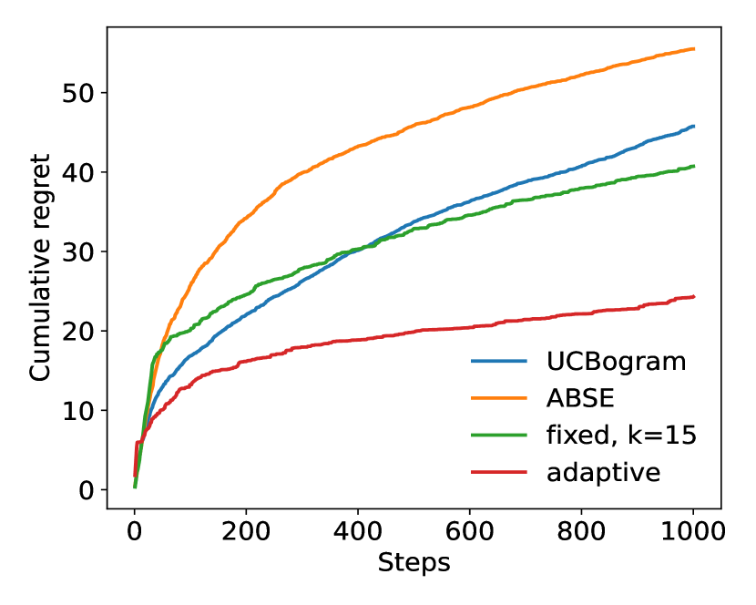
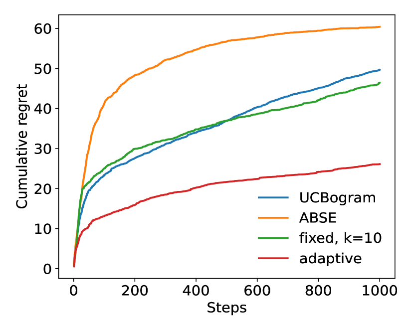
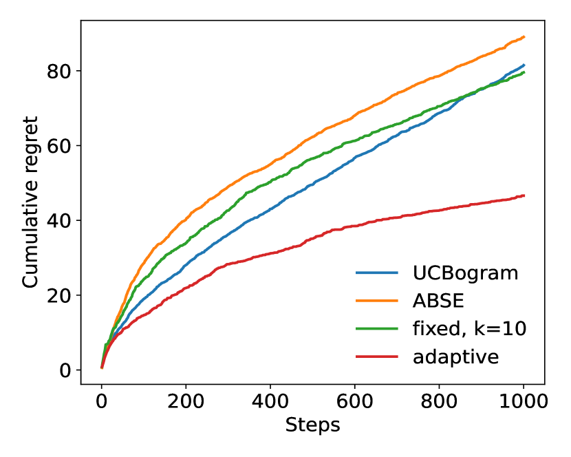
To begin with, we conduct experiments with d=1d=1. In each experiment, we run T=1,000T=1,000 steps and compare the performance of the adaptive nearest neighbor method with the UCBogram (Rigollet & Zeevi, 2010), ABSE (Perchet & Rigollet, 2013) and fixed kk nearest neighbor method. For a fair comparison, for UCBogram and ABSE, we try different numbers of bins and only pick the one with the best performance. The results are shown in Figure 1. In (a), (b), (c), and (d), the contexts follow uniform distribution in [1,1][-1,1], standard Gaussian distribution, t4t_{4} distribution, and Cauchy distribution, respectively. The uniform distribution is an example of distributions with bounded support. The Gaussian, t4t_{4} and Cauchy distribution satisfy the tail assumption (Assumption 3(a)) with β=1\beta=1, 0.80.8 and 0.50.5, respectively. In each experiment, there are two actions. For uniform and Gaussian distribution, we have η1(x)=x\eta_{1}(x)=x and η2(x)=x\eta_{2}(x)=-x. For t4t_{4} and Cauchy distribution, since they are heavy-tailed, to ensure that Assumption 3(b) is satisfied, we do not use the linear reward function. Instead, we let η1(x)=sin(x)\eta_{1}(x)=\sin(x) and η2(x)=cos(x)\eta_{2}(x)=\cos(x). To make the comparison more reliable, the values in each curve in Figure 1 are averaged over m=100m=100 random and independent trials.

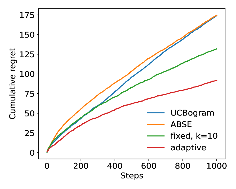
We then run experiments for two dimensional distributions. In these experiments, the context distributions are just Cartesian products of two one dimensional distributions. The two dimensional Gaussian distribution still satisfies Assumption 3(a) with β=1\beta=1, and the two dimensional t4t_{4} and Cauchy distribution satisfy Assumption 3(a) with β=2/3\beta=2/3 and 1/31/3, respectively, which are lower than the one dimensional case. The results are shown in Figure 2.

Refer to caption
(a) Uniform distribution.
Refer to caption
(b) Gaussian distribution.
Refer to caption
(c) t4t_{4} distribution.
Refer to caption
(d) Cauchy distribution.
Figure 2: Comparison of cumulative regrets of different methods for one dimensional distributions.

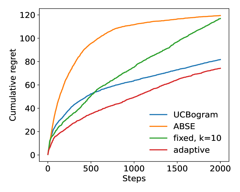
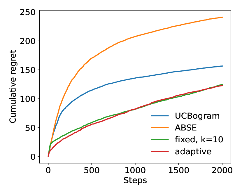
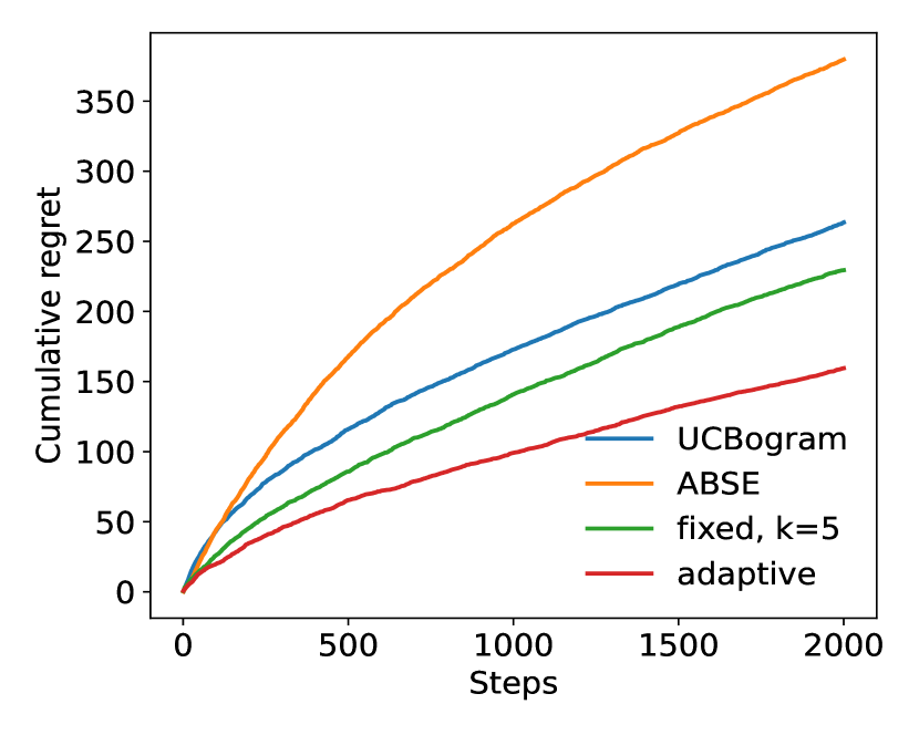
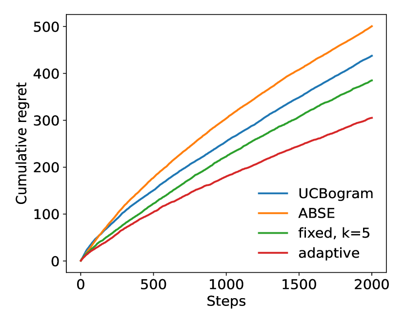
From these experiments, it can be observed that the adaptive nearest neighbor method significantly outperforms the other baselines.

7.2 Real Data

Now we run experiments using the MNIST dataset (LeCun, 1998), which contains 60,00060,000 images of handwritten digits with size 28×2828\times 28. Following the settings in (Guan & Jiang, 2018), the images are regarded as contexts, and there are 1010 actions from 0 to 99. The reward is 11 if the selected action equals the true label, and 0 otherwise. The results are shown in Figure 3. Image data have high dimensionality but low intrinsic dimensionality. Compared with bin splitting based methods (Rigollet & Zeevi, 2010; Perchet & Rigollet, 2013), nearest neighbor methods are more adaptive to local intrinsic dimension (Kpotufe, 2011). Therefore, in this experiment, we do not compare with the bin splitting based methods.

Refer to caption
Figure 3: Cumulative regrets for MNIST dataset.

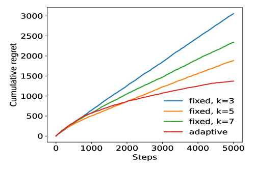
From Figure 3, the adaptive kNN method performs better than the standard kNN method with various values of kk.

8 Conclusion

This paper analyzes the contextual bandit problem that allows the context distribution to be heavy-tailed. To begin with, we have derived the minimax lower bound of the expected cumulative regret. We then show that the expected cumulative regret of the fixed kk nearest neighbor method is suboptimal compared with the minimax lower bound. To close the gap, we have proposed an adaptive nearest neighbor approach, which significantly improves the performance, and the bound of expected regret matches the minimax lower bound up to logarithm factors. Finally, we have conducted numerical experiments to validate our results.

In the future, this work can be extended in the following ways. Firstly, following existing analysis in (Gur et al., 2022), it may be meaningful to design a smoothness adaptive method that can handle any Hölder smoothness parameters. Secondly, it is worth extending current work to handle dynamic regret functions. Finally, the theories and methods developed in this paper can be extended to more complicated tasks, such as reinforcement learning (Zhao & Lai, 2024).

References

  • Abbasi-Yadkori et al. (2011) Abbasi-Yadkori, Y., Pál, D., and Szepesvári, C. Improved algorithms for linear stochastic bandits. Advances in Neural Information Processing Systems, 24, 2011.
  • Agrawal (1995) Agrawal, R. Sample mean based index policies by o (log n) regret for the multi-armed bandit problem. Advances in applied probability, 27(4):1054–1078, 1995.
  • Akhavan et al. (2024) Akhavan, A., Lounici, K., Pontil, M., and Tsybakov, A. B. Contextual continuum bandits: Static versus dynamic regret. arXiv preprint arXiv:2406.05714, 2024.
  • Audibert & Tsybakov (2007) Audibert, J.-Y. and Tsybakov, A. B. Fast learning rates for plug-in classifiers. The Annals of Statistics, pp.  608–633, 2007.
  • Auer et al. (2002) Auer, P., Cesa-Bianchi, N., and Fischer, P. Finite-time analysis of the multiarmed bandit problem. Machine learning, 47:235–256, 2002.
  • Bastani & Bayati (2020) Bastani, H. and Bayati, M. Online decision making with high-dimensional covariates. Operations Research, 68(1):276–294, 2020.
  • Bastani et al. (2021) Bastani, H., Bayati, M., and Khosravi, K. Mostly exploration-free algorithms for contextual bandits. Management Science, 67(3):1329–1349, 2021.
  • Blanchard et al. (2023) Blanchard, M., Hanneke, S., and Jaillet, P. Adversarial rewards in universal learning for contextual bandits. arXiv preprint arXiv:2302.07186, 2023.
  • Bouneffouf et al. (2020) Bouneffouf, D., Rish, I., and Aggarwal, C. Survey on applications of multi-armed and contextual bandits. In 2020 IEEE Congress on Evolutionary Computation (CEC), pp. 1–8, 2020.
  • Cai et al. (2024) Cai, C., Cai, T. T., and Li, H. Transfer learning for contextual multi-armed bandits. The Annals of Statistics, 52(1):207–232, 2024.
  • Cannings et al. (2020) Cannings, T. I., Berrett, T. B., and Samworth, R. J. Local nearest neighbour classification with applications to semi-supervised learning. The Annals of Statistics, 48(3):1789–1814, 2020.
  • Chaudhuri & Dasgupta (2014) Chaudhuri, K. and Dasgupta, S. Rates of convergence for nearest neighbor classification. In Advances in Neural Information Processing Systems, volume 27, 2014.
  • Chu et al. (2011) Chu, W., Li, L., Reyzin, L., and Schapire, R. Contextual bandits with linear payoff functions. In Proceedings of the Fourteenth International Conference on Artificial Intelligence and Statistics, pp.  208–214, 2011.
  • Döring et al. (2018) Döring, M., Györfi, L., and Walk, H. Rate of convergence of kk-nearest-neighbor classification rule. Journal of Machine Learning Research, 18(227):1–16, 2018.
  • Dudik et al. (2011) Dudik, M., Hsu, D., Kale, S., Karampatziakis, N., Langford, J., Reyzin, L., and Zhang, T. Efficient optimal learning for contextual bandits. arXiv preprint arXiv:1106.2369, 2011.
  • Durand et al. (2018) Durand, A., Achilleos, C., Iacovides, D., Strati, K., Mitsis, G. D., and Pineau, J. Contextual bandits for adapting treatment in a mouse model of de novo carcinogenesis. In Machine learning for healthcare conference, pp.  67–82, 2018.
  • Fedotov et al. (2003) Fedotov, A. A., Harremoës, P., and Topsoe, F. Refinements of pinsker’s inequality. IEEE Transactions on Information Theory, 49(6):1491–1498, 2003.
  • Gadat et al. (2016) Gadat, S., Klein, T., and Marteau, C. Classification in general finite dimensional spaces with the k nearest neighbor rule. The Annals of Statistics, pp.  982–1009, 2016.
  • Gao et al. (2018) Gao, W., Oh, S., and Viswanath, P. Demystifying fixed kk-nearest neighbor information estimators. IEEE Transactions on Information Theory, 64(8):5629–5661, 2018.
  • Garivier & Cappé (2011) Garivier, A. and Cappé, O. The kl-ucb algorithm for bounded stochastic bandits and beyond. In Proceedings of the 24th Annual Conference on Learning Theory, pp.  359–376, 2011.
  • Ghosh et al. (2024) Ghosh, A., Sankararaman, A., Ramchandran, K., Javidi, T., and Mazumdar, A. Competing bandits in non-stationary matching markets. IEEE Transactions on Information Theory, 2024.
  • Guan & Jiang (2018) Guan, M. and Jiang, H. Nonparametric stochastic contextual bandits. In Proceedings of the AAAI Conference on Artificial Intelligence, volume 32, 2018.
  • Gur et al. (2022) Gur, Y., Momeni, A., and Wager, S. Smoothness-adaptive contextual bandits. Operations Research, 70(6):3198–3216, 2022.
  • Hu et al. (2020) Hu, Y., Kallus, N., and Mao, X. Smooth contextual bandits: Bridging the parametric and non-differentiable regret regimes. In Conference on Learning Theory, pp.  2007–2010, 2020.
  • Jiang (2019) Jiang, H. Non-asymptotic uniform rates of consistency for k-nn regression. In Proceedings of the AAAI Conference on Artificial Intelligence, volume 33, pp.  3999–4006, 2019.
  • Komiyama et al. (2024) Komiyama, J., Fouché, E., and Honda, J. Finite-time analysis of globally nonstationary multi-armed bandits. Journal of Machine Learning Research, 25(112):1–56, 2024.
  • Kpotufe (2011) Kpotufe, S. k-nn regression adapts to local intrinsic dimension. In Advances in Neural Information Processing Systems, pp. 729–737, 2011.
  • Krishnamurthy et al. (2020) Krishnamurthy, A., Langford, J., Slivkins, A., and Zhang, C. Contextual bandits with continuous actions: Smoothing, zooming, and adapting. Journal of Machine Learning Research, 21(137):1–45, 2020.
  • Lai & Robbins (1985) Lai, T. L. and Robbins, H. Asymptotically efficient adaptive allocation rules. Advances in applied mathematics, 6(1):4–22, 1985.
  • Langford & Zhang (2007) Langford, J. and Zhang, T. The epoch-greedy algorithm for multi-armed bandits with side information. Advances in Neural Information Processing Systems, 20, 2007.
  • LeCun (1998) LeCun, Y. The mnist database of handwritten digits. http://yann. lecun. com/exdb/mnist/, 1998.
  • Li et al. (2010) Li, L., Chu, W., Langford, J., and Schapire, R. E. A contextual-bandit approach to personalized news article recommendation. In Proceedings of the 19th international conference on World wide web, pp.  661–670, 2010.
  • Locatelli & Carpentier (2018) Locatelli, A. and Carpentier, A. Adaptivity to smoothness in x-armed bandits. In Conference on Learning Theory, pp.  1463–1492, 2018.
  • Mai & Johansson (2021) Mai, V. V. and Johansson, M. Stability and convergence of stochastic gradient clipping: Beyond lipschitz continuity and smoothness. In International Conference on Machine Learning, pp. 7325–7335, 2021.
  • Misra et al. (2019) Misra, K., Schwartz, E. M., and Abernethy, J. Dynamic online pricing with incomplete information using multiarmed bandit experiments. Marketing Science, 38(2):226–252, 2019.
  • Perchet & Rigollet (2013) Perchet, V. and Rigollet, P. The multi-armed bandit problem with covariates. The Annals of Statistics, 41(2):693–721, 2013.
  • Qian & Yang (2016) Qian, W. and Yang, Y. Kernel estimation and model combination in a bandit problem with covariates. Journal of Machine Learning Research, 17(149):1–37, 2016.
  • Qian et al. (2023) Qian, W., Ing, C.-K., and Liu, J. Adaptive algorithm for multi-armed bandit problem with high-dimensional covariates. Journal of the American Statistical Association, pp.  1–13, 2023.
  • Reeve et al. (2018) Reeve, H., Mellor, J., and Brown, G. The k-nearest neighbour ucb algorithm for multi-armed bandits with covariates. In Algorithmic Learning Theory, pp.  725–752, 2018.
  • Rigollet & Zeevi (2010) Rigollet, P. and Zeevi, A. Nonparametric bandits with covariates. 23th Annual Conference on Learning Theory, pp.  54, 2010.
  • Robbins (1952) Robbins, H. Some aspects of the sequential design of experiments. Bulletin of the American Mathematical Society, 58(5):527–535, 1952.
  • Slivkins (2014) Slivkins, A. Contextual bandits with similarity information. Journal of Machine Learning Research, 15:2533–2568, 2014.
  • Suk (2024) Suk, J. Adaptive smooth non-stationary bandits. arXiv preprint arXiv:2407.08654, 2024.
  • Suk & Kpotufe (2023) Suk, J. and Kpotufe, S. Tracking most significant shifts in nonparametric contextual bandits. Advances in Neural Information Processing Systems, 36:6202–6241, 2023.
  • Tsybakov (2009) Tsybakov, A. B. Introduction to Nonparametric Estimation. 2009.
  • Wanigasekara & Yu (2019) Wanigasekara, N. and Yu, C. L. Nonparametric contextual bandits in an unknown metric space. Advances in Neural Information Processing Systems, 32:14684–14694, 2019.
  • Woodroofe (1979) Woodroofe, M. A one-armed bandit problem with a concomitant variable. Journal of the American Statistical Association, 74(368):799–806, 1979.
  • Yang & Zhu (2002) Yang, Y. and Zhu, D. Randomized allocation with nonparametric estimation for a multi-armed bandit problem with covariates. The Annals of Statistics, 30(1):100–121, 2002.
  • Zangerle & Bauer (2022) Zangerle, E. and Bauer, C. Evaluating recommender systems: survey and framework. ACM Computing Surveys, 55(8):1–38, 2022.
  • Zhao & Lai (2021a) Zhao, P. and Lai, L. Efficient classification with adaptive knn. In Proceedings of the AAAI Conference on Artificial Intelligence, volume 35, pp.  11007–11014, 2021a.
  • Zhao & Lai (2021b) Zhao, P. and Lai, L. Minimax rate optimal adaptive nearest neighbor classification and regression. IEEE Transactions on Information Theory, 67(5):3155–3182, 2021b.
  • Zhao & Lai (2022) Zhao, P. and Lai, L. Analysis of knn density estimation. IEEE Transactions on Information Theory, 68(12):7971–7995, 2022.
  • Zhao & Lai (2024) Zhao, P. and Lai, L. Minimax optimal q learning with nearest neighbors. IEEE Transactions on Information Theory, 2024.
  • Zhao & Wan (2024) Zhao, P. and Wan, Z. Robust nonparametric regression under poisoning attack. In Proceedings of the AAAI Conference on Artificial Intelligence, volume 38, pp.  17007–17015, 2024.
  • Zhou et al. (2017) Zhou, Q., Zhang, X., Xu, J., and Liang, B. Large-scale bandit approaches for recommender systems. In Neural Information Processing: 24th International Conference, ICONIP 2017, Guangzhou, China, November 14-18, 2017, Proceedings, Part I 24, pp.  811–821. Springer, 2017.
  • Zhu et al. (2022) Zhu, Y., Foster, D. J., Langford, J., and Mineiro, P. Contextual bandits with large action spaces: Made practical. In International Conference on Machine Learning, pp. 27428–27453. PMLR, 2022.

Appendix A Examples of Heavy-tailed Distributions

This section explains Example 1 and 2 in the paper. For Example 1,

P(f(𝐗)<t)=𝒳f(𝐱)𝟏(f(𝐱)<t)𝑑𝐱tV(𝒳).\displaystyle\text{P}(f(\mathbf{X})<t)=\int_{\mathcal{X}}f(\mathbf{x})\mathbf{1}(f(\mathbf{x})<t)d\mathbf{x}\leq tV(\mathcal{X}). (23)

For Example 2, from Hölder’s inequality,

f1β(𝐱)𝑑𝐱=f1β(𝐱)(1+𝐱γ)11+𝐱γ\displaystyle\int f^{1-\beta}(\mathbf{x})d\mathbf{x}=\int f^{1-\beta}(\mathbf{x})(1+\left\lVert\mathbf{x}\right\rVert^{\gamma})\frac{1}{1+\left\lVert\mathbf{x}\right\rVert^{\gamma}}
(f(𝐱)(1+𝐱γ)11β𝑑𝐱)1β((1+𝐱γ)1β𝑑𝐱)β.\displaystyle\leq\left(\int f(\mathbf{x})(1+\left\lVert\mathbf{x}\right\rVert^{\gamma})^{\frac{1}{1-\beta}}d\mathbf{x}\right)^{1-\beta}\left(\int(1+\left\lVert\mathbf{x}\right\rVert^{\gamma})^{-\frac{1}{\beta}}d\mathbf{x}\right)^{\beta}.

Let γ=p(1β)\gamma=p(1-\beta), then (f(𝐱)(1+𝐱γ)11β𝑑𝐱)1β<\left(\int f(\mathbf{x})(1+\left\lVert\mathbf{x}\right\rVert^{\gamma})^{\frac{1}{1-\beta}}d\mathbf{x}\right)^{1-\beta}<\infty. If β<p/(p+d)\beta<p/(p+d), then γ/β>d\gamma/\beta>d, thus ((1+𝐱γ)1β𝑑𝐱)β<\left(\int(1+\left\lVert\mathbf{x}\right\rVert^{\gamma})^{-\frac{1}{\beta}}d\mathbf{x}\right)^{\beta}<\infty. Hence f1β(𝐱)𝑑𝐱<\int f^{1-\beta}(\mathbf{x})d\mathbf{x}<\infty, and

P(f(𝐗)<t)=P(fβ(𝐗)>tβ)tβ𝔼[fβ(𝐗)]=tβf1β(𝐱)𝑑𝐱.\displaystyle\text{P}(f(\mathbf{X})<t)=\text{P}(f^{-\beta}(\mathbf{X})>t^{-\beta})\leq t^{\beta}\mathbb{E}[f^{-\beta}(\mathbf{X})]=t^{\beta}\int f^{1-\beta}(\mathbf{x})d\mathbf{x}. (25)

Therefore for all β<p/(p+d)\beta<p/(p+d), Assumption 3(a) holds with some finite CβC_{\beta}.

For subgaussian or subexponential random variables, 𝔼[𝐗p]<\mathbb{E}[\left\lVert\mathbf{X}\right\rVert^{p}]<\infty holds for any pp, thus Assumption 3(a) holds for β\beta arbitrarily close to 11.

Appendix B Expected Sample Density

In this section, we define expected sample density, which is then used in the later analysis. Throughout this section, denote x(j)x(j) as the value of jj-th component of vector 𝐱\mathbf{x}.

Definition 1.

(expected sample density) qa:𝒳q_{a}:\mathcal{X}\rightarrow\mathbb{R} is defined as the function such that for all S𝒳S\subseteq\mathcal{X},

𝔼[t=1T𝟏(𝐗tS,At=a)]=Sqa(𝐱)𝑑𝐱.\displaystyle\mathbb{E}\left[\sum_{t=1}^{T}\mathbf{1}(\mathbf{X}_{t}\in S,A_{t}=a)\right]=\int_{S}q_{a}(\mathbf{x})d\mathbf{x}. (26)

To show the existence of qaq_{a}, define

Qa(𝐱)=𝔼[t=1T𝟏(𝐗t{u|u(1)x(1),,u(d)x(d)},At=a)].\displaystyle Q_{a}(\mathbf{x})=\mathbb{E}\left[\sum_{t=1}^{T}\mathbf{1}(\mathbf{X}_{t}\in\{u|u(1)\leq x(1),\ldots,u(d)\leq x(d)\},A_{t}=a)\right]. (27)

Then let

qa(𝐱)=dQax(1)x(d)|x,\displaystyle q_{a}(\mathbf{x})=\left.\frac{\partial^{d}Q_{a}}{\partial x(1)\ldots\partial x(d)}\right|_{x}, (28)

and then (26) is satisfied for all S𝒳S\subseteq\mathcal{X}.

Then we show the following basic lemmas.

Lemma 1.

Regardless of η\eta, qaq_{a} satisfies

qa(𝐱)Tf(𝐱)\displaystyle q_{a}(\mathbf{x})\leq Tf(\mathbf{x}) (29)

for almost all 𝐱𝒳\mathbf{x}\in\mathcal{X}.

Proof.

Note that P(𝐗tS)=Sf(𝐱)𝑑𝐱\text{P}(\mathbf{X}_{t}\in S)=\int_{S}f(\mathbf{x})d\mathbf{x}. Therefore for all set SS,

𝔼[t=1T𝟏(𝐗tS,At=a)]TSf(𝐱)𝑑𝐱.\displaystyle\mathbb{E}\left[\sum_{t=1}^{T}\mathbf{1}(\mathbf{X}_{t}\in S,A_{t}=a)\right]\leq T\int_{S}f(\mathbf{x})d\mathbf{x}. (30)

From (26) and (30), Sqa(𝐱)𝑑𝐱TSf(𝐱)𝑑𝐱\int_{S}q_{a}(\mathbf{x})d\mathbf{x}\leq T\int_{S}f(\mathbf{x})d\mathbf{x} for all SS. Therefore qa(𝐱)Tf(𝐱)q_{a}(\mathbf{x})\leq Tf(\mathbf{x}) for almost all 𝐱𝒳\mathbf{x}\in\mathcal{X}. ∎

Lemma 2.

R=a𝒜RaR=\sum_{a\in\mathcal{A}}R_{a}, in which RaR_{a} is defined as

Ra:=𝒳(η(𝐱)ηa(𝐱))qa(𝐱)𝑑𝐱.\displaystyle R_{a}:=\int_{\mathcal{X}}(\eta^{*}(\mathbf{x})-\eta_{a}(\mathbf{x}))q_{a}(\mathbf{x})d\mathbf{x}. (31)
Proof.
R\displaystyle R =\displaystyle= 𝔼[t=1T(η(𝐗t)ηAt(𝐗t))]\displaystyle\mathbb{E}\left[\sum_{t=1}^{T}\left(\eta^{*}(\mathbf{X}_{t})-\eta_{A_{t}}(\mathbf{X}_{t})\right)\right] (32)
=\displaystyle= a𝒜𝔼[t=1T(η(𝐗t)ηa(𝐗t))𝟏(At=a)]\displaystyle\sum_{a\in\mathcal{A}}\mathbb{E}\left[\sum_{t=1}^{T}(\eta^{*}(\mathbf{X}_{t})-\eta_{a}(\mathbf{X}_{t}))\mathbf{1}(A_{t}=a)\right]
=\displaystyle= a𝒜𝒳(η(𝐱)ηa(𝐱))qa(𝐱)𝑑𝐱.\displaystyle\sum_{a\in\mathcal{A}}\int_{\mathcal{X}}\left(\eta^{*}(\mathbf{x})-\eta_{a}(\mathbf{x})\right)q_{a}(\mathbf{x})d\mathbf{x}.

The proof is complete. ∎

Appendix C Proof of Theorem 1

Recall that

R=𝔼[t=1T(η(𝐗t)ηAt(𝐗t))].\displaystyle R=\mathbb{E}\left[\sum_{t=1}^{T}(\eta^{*}(\mathbf{X}_{t})-\eta_{A_{t}}(\mathbf{X}_{t}))\right]. (33)

Now we define

S=𝔼[t=1T𝟏(ηAt(𝐗t)<η(𝐗t))]\displaystyle S=\mathbb{E}\left[\sum_{t=1}^{T}\mathbf{1}(\eta_{A_{t}}(\mathbf{X}_{t})<\eta^{*}(\mathbf{X}_{t}))\right] (34)

as the expected number of steps with suboptimal actions.

The following lemma characterizes the relationship between SS and RR.

Lemma 3.

There exists a constant C0C_{0}, such that

RC0Sα+1αT1α.\displaystyle R\geq C_{0}S^{\frac{\alpha+1}{\alpha}}T^{-\frac{1}{\alpha}}. (35)
Proof.

The proof of Lemma 3 follows the proof of Lemma 3.1 in (Rigollet & Zeevi, 2010). For completeness and consistency of notations, we show the proof in Appendix I.10. ∎

From now on, we only discuss the case with only two actions, such that 𝒜={1,1}\mathcal{A}=\{1,-1\}. Construct BB disjoint balls with centers 𝐜1,,𝐜B\mathbf{c}_{1},\ldots,\mathbf{c}_{B} and radius hh. Let

f(𝐱)=j=1B𝟏(𝐱Bj),\displaystyle f(\mathbf{x})=\sum_{j=1}^{B}\mathbf{1}(\mathbf{x}\in B_{j}), (36)

in which Bj={𝐱|𝐱𝐜jh}B_{j}=\{\mathbf{x}^{\prime}|\left\lVert\mathbf{x}^{\prime}-\mathbf{c}_{j}\right\rVert\leq h\} is the jj-th ball. To ensure that the pdf defined above is normalized (i.e. f(𝐱)𝑑𝐱=1\int f(\mathbf{x})d\mathbf{x}=1), BB and hh need to satisfy

Bvdhd=1,\displaystyle Bv_{d}h^{d}=1, (37)

in which vdv_{d} is the volume of dd dimensional unit ball.

Let η1(𝐱)=η(𝐱)\eta_{1}(\mathbf{x})=\eta(\mathbf{x}) and η2(𝐱)=0\eta_{2}(\mathbf{x})=0, with

η(𝐱)=j=1Kvjh𝟏(𝐱B(cj,h)),\displaystyle\eta(\mathbf{x})=\sum_{j=1}^{K}v_{j}h\mathbf{1}(\mathbf{x}\in B(c_{j},h)), (38)

in which vj{1,1}v_{j}\in\{-1,1\} for j=1,,Kj=1,\ldots,K. To satisfy the margin assumption (Assumption 1(a)), note that

P(0<|η(𝐗)|t){Kvdhdifth0ift<h.\displaystyle\text{P}(0<|\eta(\mathbf{X})|\leq t)\leq\left\{\begin{array}[]{ccc}Kv_{d}h^{d}&\text{if}&t\geq h\\ 0&\text{if}&t<h.\end{array}\right. (41)

Note that for any suboptimal action aa, η(𝐱)ηa(𝐱)=|η(𝐱)|\eta^{*}(\mathbf{x})-\eta_{a}(\mathbf{x})=|\eta(\mathbf{x})|. Assumption 1(a) requires that P(0<|η(𝐗)|t)Cαtα\text{P}(0<|\eta(\mathbf{X})|\leq t)\leq C_{\alpha}t^{\alpha}. Therefore, it suffices to ensure that

Kvdhd=Cαhα.\displaystyle Kv_{d}h^{d}=C_{\alpha}h^{\alpha}. (42)

Then

S\displaystyle S =\displaystyle= j=1Kt=1TP(𝐗tBj,Ata(𝐗t))\displaystyle\sum_{j=1}^{K}\sum_{t=1}^{T}\text{P}(\mathbf{X}_{t}\in B_{j},A_{t}\neq a^{*}(\mathbf{X}_{t})) (43)
\displaystyle\geq j=1Kt=1TBjf(𝐱)P(Ata(𝐱)|𝐗t=x)𝑑𝐱\displaystyle\sum_{j=1}^{K}\sum_{t=1}^{T}\int_{B_{j}}f(\mathbf{x})\text{P}(A_{t}\neq a^{*}(\mathbf{x})|\mathbf{X}_{t}=x)d\mathbf{x}
=\displaystyle= j=1Kt=1TBjf(𝐱)P(Atvj|𝐗t=x)𝑑𝐱\displaystyle\sum_{j=1}^{K}\sum_{t=1}^{T}\int_{B_{j}}f(\mathbf{x})\text{P}(A_{t}\neq v_{j}|\mathbf{X}_{t}=x)d\mathbf{x}
=\displaystyle= j=1kt=1T𝔼[Bjf(𝐱)𝟏(π(x;𝐗1:t1,Y1:t1)vj)𝑑𝐱].\displaystyle\sum_{j=1}^{k}\sum_{t=1}^{T}\mathbb{E}\left[\int_{B_{j}}f(\mathbf{x})\mathbf{1}(\pi(x;\mathbf{X}_{1:t-1},Y_{1:t-1})\neq v_{j})d\mathbf{x}\right].

Define

v^j(t)=sign(Bjf(𝐱)π(x;𝐗1:t1,Y1:t1)𝑑𝐱).\displaystyle\hat{v}_{j}(t)=\operatorname{sign}\left(\int_{B_{j}}f(\mathbf{x})\pi(x;\mathbf{X}_{1:t-1},Y_{1:t-1})d\mathbf{x}\right). (44)

Then

Bjf(𝐱)𝟏(π(x;𝐗1:t1,Y1:t1)v^j(t))𝑑𝐱Bjf(𝐱)𝟏(π(x;𝐗1:t1,Y1:t1)=v^j(t))𝑑𝐱.\displaystyle\int_{B_{j}}f(\mathbf{x})\mathbf{1}(\pi(x;\mathbf{X}_{1:t-1},Y_{1:t-1})-\hat{v}_{j}(t))d\mathbf{x}\geq\int_{B_{j}}f(\mathbf{x})\mathbf{1}\left(\pi(x;\mathbf{X}_{1:t-1},Y_{1:t-1})=-\hat{v}_{j}(t)\right)d\mathbf{x}. (45)

Since

Bjf(𝐱)𝟏(π(x;𝐗1:t1,Y1:t1)v^j(t))𝑑𝐱+Bjf(𝐱)𝟏(π(x;𝐗1:t1,Y1:t1)=v^j(t))𝑑𝐱\displaystyle\int_{B_{j}}f(\mathbf{x})\mathbf{1}\left(\pi(x;\mathbf{X}_{1:t-1},Y_{1:t-1})-\hat{v}_{j}(t)\right)d\mathbf{x}+\int_{B_{j}}f(\mathbf{x})\mathbf{1}\left(\pi(x;\mathbf{X}_{1:t-1},Y_{1:t-1})=-\hat{v}_{j}(t)\right)d\mathbf{x}
=Bjf(𝐱)𝑑𝐱,\displaystyle=\int_{B_{j}}f(\mathbf{x})d\mathbf{x}, (46)

we have

Bjf(𝐱)𝟏(π(x;𝐗1:t1,Y1:t1)=v^j(t))𝑑𝐱12Bjf(𝐱)𝑑𝐱.\displaystyle\int_{B_{j}}f(\mathbf{x})\mathbf{1}\left(\pi(x;\mathbf{X}_{1:t-1},Y_{1:t-1})=\hat{v}_{j}(t)\right)d\mathbf{x}\geq\frac{1}{2}\int_{B_{j}}f(\mathbf{x})d\mathbf{x}. (47)

If v^j(t)vj\hat{v}_{j}(t)\neq v_{j}, then

Bjf(𝐱)𝟏(π(x;𝐗1:t1,Y1:t1)vj)𝑑𝐱12Bjf(𝐱)𝑑𝐱.\displaystyle\int_{B_{j}}f(\mathbf{x})\mathbf{1}\left(\pi(x;\mathbf{X}_{1:t-1},Y_{1:t-1})\neq v_{j}\right)d\mathbf{x}\geq\frac{1}{2}\int_{B_{j}}f(\mathbf{x})d\mathbf{x}. (48)

Therefore, from (43),

S\displaystyle S \displaystyle\geq j=1Kt=1T12P(v^j(t)vj)Bjf(𝐱)𝑑𝐱\displaystyle\sum_{j=1}^{K}\sum_{t=1}^{T}\frac{1}{2}\text{P}(\hat{v}_{j}(t)\neq v_{j})\int_{B_{j}}f(\mathbf{x})d\mathbf{x} (49)
\displaystyle\geq j=1Kt=1T12vdhdP(v^j(t)vj).\displaystyle\sum_{j=1}^{K}\sum_{t=1}^{T}\frac{1}{2}v_{d}h^{d}\text{P}(\hat{v}_{j}(t)\neq v_{j}).

Note that the error probability of hypothesis testing between distance pp and qq is at least (1𝕋𝕍(p,q))/2(1-\mathbb{TV}(p,q))/2, in which 𝕋𝕍\mathbb{TV} denotes the total variation distance. Let (V1,,VK)(V_{1},\ldots,V_{K}) be a vector of KK random variables taking values from {1,1}K\{-1,1\}^{K} randomly. In other words, P(Vj=1)=P(Vj=1)=1/2\text{P}(V_{j}=1)=\text{P}(V_{j}=-1)=1/2, and VjV_{j} for different jj are i.i.d. Denote XY|Vj=vj\mathbb{P}_{XY|V_{j}=v_{j}} as the distribution of XX and YY conditional on Vj=vjV_{j}=v_{j}. Moreover, XY|Vj=vjt1\mathbb{P}_{XY|V_{j}=v_{j}}^{t-1} means the distribution of XX and YY of the first t1t-1 samples conditional on Vj=vjV_{j}=v_{j}. Then

P(v^j(t)vj)\displaystyle\text{P}(\hat{v}_{j}(t)\neq v_{j}) \displaystyle\geq 12(1𝕋𝕍(XY|vj=1t1||XY|Vj=1t1))\displaystyle\frac{1}{2}\left(1-\mathbb{TV}\left(\mathbb{P}_{XY|v_{j}=1}^{t-1}||\mathbb{P}_{XY|V_{j}=-1}^{t-1}\right)\right) (50)
\displaystyle\geq 12(112D(XY|Vj=1t1||XY|Vj=1t1)),\displaystyle\frac{1}{2}\left(1-\sqrt{\frac{1}{2}D\left(\mathbb{P}_{XY|V_{j}=1}^{t-1}||\mathbb{P}_{XY|V_{j}=-1}^{t-1}\right)}\right),

in which the second step uses Pinsker’s inequality (Fedotov et al., 2003), and D(p||q)D(p||q) denotes the Kullback-Leibler (KL) divergence between distributions pp and qq. Note that the KL divergence between the conditional distribution is bounded by

D(Y|X,Vj=1||Y|X,Vj=1)12(η1(𝐱)η2(𝐱))212η2(𝐱)=12h2\displaystyle D(\mathbb{P}_{Y|X,V_{j}=1}||\mathbb{P}_{Y|X,V_{j}=-1})\leq\frac{1}{2}(\eta_{1}(\mathbf{x})-\eta_{2}(\mathbf{x}))^{2}\leq\frac{1}{2}\eta^{2}(\mathbf{x})=\frac{1}{2}h^{2} (51)

for 𝐱Bj\mathbf{x}\in B_{j}. Therefore

D(XY|Vj=1||XY|Vj=1)\displaystyle D(\mathbb{P}_{XY|V_{j}=1}||\mathbb{P}_{XY|V_{j}=-1}) =\displaystyle= f(𝐱)D(Y|X,Vj=1||Y|X,Vj=1)d𝐱\displaystyle\int f(\mathbf{x})D(\mathbb{P}_{Y|X,V_{j}=1}||\mathbb{P}_{Y|X,V_{j}=-1})d\mathbf{x} (52)
\displaystyle\leq Bj12h2𝑑𝐱\displaystyle\int_{B_{j}}\frac{1}{2}h^{2}d\mathbf{x}
=\displaystyle= 12vdhd+2.\displaystyle\frac{1}{2}v_{d}h^{d+2}.

Hence, from (50),

P(v^j(t)vj)\displaystyle\text{P}(\hat{v}_{j}(t)\neq v_{j}) \displaystyle\geq 12(114(t1)vdhd+2)\displaystyle\frac{1}{2}\left(1-\sqrt{\frac{1}{4}(t-1)v_{d}h^{d+2}}\right) (53)
\displaystyle\geq 12(112Tvdhd+2).\displaystyle\frac{1}{2}\left(1-\frac{1}{2}\sqrt{Tv_{d}h^{d+2}}\right).

Recall (49),

S\displaystyle S \displaystyle\geq 14j=1Kt=1Tvdhd(112Tvdhd+2)\displaystyle\frac{1}{4}\sum_{j=1}^{K}\sum_{t=1}^{T}v_{d}h^{d}\left(1-\frac{1}{2}\sqrt{Tv_{d}h^{d+2}}\right) (54)
=\displaystyle= 14KTvdhd(112Tvdhd+2)\displaystyle\frac{1}{4}KTv_{d}h^{d}\left(1-\frac{1}{2}\sqrt{Tv_{d}h^{d+2}}\right)
=\displaystyle= 14CαThα(112Tvdhd+2),\displaystyle\frac{1}{4}C_{\alpha}Th^{\alpha}\left(1-\frac{1}{2}\sqrt{Tv_{d}h^{d+2}}\right),

in which the last step comes from (42).

Let hT1d+2h\sim T^{-\frac{1}{d+2}}, then

ST1αd+2.\displaystyle S\gtrsim T^{1-\frac{\alpha}{d+2}}. (55)

From Lemma 3,

R\displaystyle R \displaystyle\gtrsim T(1αd+2)α+1αT1αT1α+1d+2\displaystyle T^{\left(1-\frac{\alpha}{d+2}\right)\frac{\alpha+1}{\alpha}}T^{-\frac{1}{\alpha}}\sim T^{1-\frac{\alpha+1}{d+2}} (56)
\displaystyle\sim T1α+1d+2.\displaystyle T^{1-\frac{\alpha+1}{d+2}}.

Appendix D Proof of Theorem 2

In this section, we derive the minimax lower bound of the expected regret with unbounded support. Recall that in the case with bounded support of contexts (Proof of Theorem 1 in Appendix C), we construct BB disjoint balls with pdf f(𝐱)=1f(\mathbf{x})=1 for all 𝐱𝒳\mathbf{x}\in\mathcal{X}. Now for the case with unbounded support, the distribution of context has tails, on which the pdf f(𝐱)f(\mathbf{x}) is small. Therefore, we modify the construction of balls as follows. We now construct B+1B+1 disjoint balls with center 𝐜0,,𝐜B\mathbf{c}_{0},\ldots,\mathbf{c}_{B}, such that

B0\displaystyle B_{0} =\displaystyle= {𝐱|𝐱𝐜0r0},\displaystyle\{\mathbf{x}^{\prime}|\left\lVert\mathbf{x}^{\prime}-\mathbf{c}_{0}\right\rVert\leq r_{0}\}, (57)
Bj\displaystyle B_{j} =\displaystyle= {𝐱|𝐱𝐜jh}.\displaystyle\{\mathbf{x}^{\prime}|\left\lVert\mathbf{x}^{\prime}-\mathbf{c}_{j}\right\rVert\leq h\}. (58)

Let

η(𝐱)=j=1Kvjh𝟏(𝐱B(𝐜j,h)),\displaystyle\eta(\mathbf{x})=\sum_{j=1}^{K}v_{j}h\mathbf{1}(\mathbf{x}\in B(\mathbf{c}_{j},h)), (59)

in which vj{0,1}v_{j}\in\{0,1\} is unknown, and

f(𝐱)=𝟏(𝐱B0)+j=1Bm𝟏(𝐱Bj),\displaystyle f(\mathbf{x})=\mathbf{1}(\mathbf{x}\in B_{0})+\sum_{j=1}^{B}m\mathbf{1}(\mathbf{x}\in B_{j}), (60)

in which m1m\ll 1 will be determined later. Here we construct one ball that denotes the center region which has the most of probability mass, as well as BB balls that denotes the tail region. For simplicity, we let η(𝐱)=0\eta(\mathbf{x})=0 at the largest ball B0B_{0}, and only

To satisfy the margin condition (i.e. Assumption 1(a)), note that now

P(0<|η(𝐗)|<t)\displaystyle\text{P}(0<|\eta(\mathbf{X})|<t) \displaystyle\leq {mKvdhdift>h0ifth.\displaystyle\left\{\begin{array}[]{ccc}mKv_{d}h^{d}&\text{if}&t>h\\ 0&\text{if}&t\leq h.\end{array}\right. (63)

The right hand side of (63) can not exceed CαtαC_{\alpha}t^{\alpha}, which requires

mKvdhdCαhα.\displaystyle mKv_{d}h^{d}\leq C_{\alpha}h^{\alpha}. (64)

Moreover, to satisfy the tail assumption (Assumption 3(a)), note that

P(f(𝐗)<t)\displaystyle\text{P}(f(\mathbf{X})<t) \displaystyle\leq {mKvdhdift>m0iftm.\displaystyle\left\{\begin{array}[]{ccc}mKv_{d}h^{d}&\text{if}&t>m\\ 0&\text{if}&t\leq m.\end{array}\right. (67)

The right hand side of (67) can not exceed CβtβC_{\beta}t^{\beta}, which requires

mKvdhdCβmβ.\displaystyle mKv_{d}h^{d}\lesssim C_{\beta}m^{\beta}. (68)

Following (49), SS can be lower bounded by

S\displaystyle S \displaystyle\geq j=1Kt=1T12P(v^j(t)vj)Bjf(𝐱)𝑑𝐱\displaystyle\sum_{j=1}^{K}\sum_{t=1}^{T}\frac{1}{2}\text{P}(\hat{v}_{j}(t)\neq v_{j})\int_{B_{j}}f(\mathbf{x})d\mathbf{x} (69)
=\displaystyle= j=1Kt=1T12mvdhdP(v^j(t)vj)\displaystyle\sum_{j=1}^{K}\sum_{t=1}^{T}\frac{1}{2}mv_{d}h^{d}\text{P}(\hat{v}_{j}(t)\neq v_{j})
\displaystyle\geq 14j=1Kt=1Tmvdhd(112D(XY|Vj=1||XY|Vj=1))\displaystyle\frac{1}{4}\sum_{j=1}^{K}\sum_{t=1}^{T}mv_{d}h^{d}\left(1-\sqrt{\frac{1}{2}D(\mathbb{P}_{XY|V_{j}=1}||\mathbb{P}_{XY|V_{j}=-1})}\right)
\displaystyle\geq 14j=1Kt=1Tmvdhd(112Tmvdhd+2).\displaystyle\frac{1}{4}\sum_{j=1}^{K}\sum_{t=1}^{T}mv_{d}h^{d}\left(1-\frac{1}{2}\sqrt{Tmv_{d}h^{d+2}}\right).

From (69), we pick mm and hh to ensure that

Tmvdhd+2<12.\displaystyle Tmv_{d}h^{d+2}<\frac{1}{2}. (70)

Then under three conditions (64), (68) and (70),

SKTmhd.\displaystyle S\gtrsim KTmh^{d}. (71)

It remains to determine the value of mm, hh and KK based on these three conditions. Let

h(Tm)1d+2,\displaystyle h\sim(Tm)^{-\frac{1}{d+2}}, (72)
mTαα+β(d+2),\displaystyle m\sim T^{-\frac{\alpha}{\alpha+\beta(d+2)}}, (73)

and

Khαd/m,\displaystyle K\sim h^{\alpha-d}/m, (74)

then

SThαT1αβα+β(d+2).\displaystyle S\gtrsim Th^{\alpha}\sim T^{1-\frac{\alpha\beta}{\alpha+\beta(d+2)}}. (75)

Based on Lemma 3,

RS1+ααT1αT1(α+1)βα+β(d+2).\displaystyle R\gtrsim S^{\frac{1+\alpha}{\alpha}}T^{-\frac{1}{\alpha}}\sim T^{1-\frac{(\alpha+1)\beta}{\alpha+\beta(d+2)}}. (76)

It remains to show that RT1βR\gtrsim T^{1-\beta}. Let h1h\sim 1, KT1βK\sim T^{1-\beta} and m1/Tm\sim 1/T, the conditions (64), (68) and (70) are still satisfied. In this case,

ST1β.\displaystyle S\gtrsim T^{1-\beta}. (77)

Direct transformation using Lemma 3 yields suboptimal bound. Intuitively, for the case with heavy tails (i.e. β\beta is small), the regret mainly occur at the tail of the context distribution. Therefore, we bound the expected regret again.

R\displaystyle R =\displaystyle= 𝔼[t=1T(η(𝐗t)ηAt(𝐗t))]\displaystyle\mathbb{E}\left[\sum_{t=1}^{T}(\eta^{*}(\mathbf{X}_{t})-\eta_{A_{t}}(\mathbf{X}_{t}))\right] (78)
=(a)\displaystyle\overset{(a)}{=} 𝔼[t=1Th𝟏(ηAt(𝐗t)<η(𝐗t))]\displaystyle\mathbb{E}\left[\sum_{t=1}^{T}h\mathbf{1}\left(\eta_{A_{t}}(\mathbf{X}_{t})<\eta^{*}(\mathbf{X}_{t})\right)\right]
=(b)\displaystyle\overset{(b)}{=} ST1β.\displaystyle S\gtrsim T^{1-\beta}.

(a) comes from the construction of η\eta in (59). (b) holds since we set h=1h=1 here.

Combine (76) and (78),

RT1(α+1)βα+β(d+2)+T1β.\displaystyle R\gtrsim T^{1-\frac{(\alpha+1)\beta}{\alpha+\beta(d+2)}}+T^{1-\beta}. (79)

Appendix E Proof of Theorem 3

To begin with, we show the following lemma.

Lemma 4.

For all u>0u>0,

P(supx,a|1ki𝒩t(𝐱,a)Wi|>u)dT2d|𝒜|eku22σ2.\displaystyle\text{P}\left(\underset{x,a}{\sup}\left|\frac{1}{k}\sum_{i\in\mathcal{N}_{t}(\mathbf{x},a)}W_{i}\right|>u\right)\leq dT^{2d}|\mathcal{A}|e^{-\frac{ku^{2}}{2\sigma^{2}}}. (80)
Proof.

The proof is shown in Appendix I.1. ∎

From Lemma 4, recall the definition of bb in (10),

P(supx,a|1ki𝒩t(𝐱,a)Wi|>b)1T2.\displaystyle\text{P}\left(\underset{x,a}{\sup}\left|\frac{1}{k}\sum_{i\in\mathcal{N}_{t}(\mathbf{x},a)}W_{i}\right|>b\right)\leq\frac{1}{T^{2}}. (81)

Therefore, with probability 11/T1-1/T, for all 𝐱𝒳\mathbf{x}\in\mathcal{X}, a𝒜a\in\mathcal{A} and t=1,,Tt=1,\ldots,T, |i𝒩t(𝐱,a)Wi|/kb|\sum_{i\in\mathcal{N}_{t}(\mathbf{x},a)}W_{i}|/k\leq b. Denote EE as the event such that |i𝒩t(𝐱,a)Wi|/kb|\sum_{i\in\mathcal{N}_{t}(\mathbf{x},a)}W_{i}|/k\leq b, x,a,t\forall x,a,t, then

P(E)\displaystyle\text{P}(E) =\displaystyle= P(t=1T{supx,a|1ki𝒩t(𝐱,a)Wi|b})\displaystyle\text{P}\left(\cap_{t=1}^{T}\left\{\sup_{x,a}\left|\frac{1}{k}\sum_{i\in\mathcal{N}_{t}(\mathbf{x},a)}W_{i}\right|\leq b\right\}\right) (82)
=\displaystyle= 1P(t=1T{supx,a|1ki𝒩t(𝐱,a)Wi|>b})\displaystyle 1-\text{P}\left(\cap_{t=1}^{T}\left\{\sup_{x,a}\left|\frac{1}{k}\sum_{i\in\mathcal{N}_{t}(\mathbf{x},a)}W_{i}\right|>b\right\}\right)
\displaystyle\geq 1T1T211T.\displaystyle 1-T\frac{1}{T^{2}}\geq 1-\frac{1}{T}.

Recall the calculation of UCB in (9). Based on Lemma 4, we then show some properties of the UCB in (9).

Lemma 5.

Under EE, if |{i<t|Ai=a}|k|\{i<t|A_{i}=a\}|\geq k, then

ηa(t)η^a,t(𝐱)ηa(𝐱)+2b+2Lρa,t(𝐱).\displaystyle\eta_{a}(t)\leq\hat{\eta}_{a,t}(\mathbf{x})\leq\eta_{a}(\mathbf{x})+2b+2L\rho_{a,t}(\mathbf{x}). (83)
Proof.

The proof is shown in Appendix I.2. ∎

We then bound the number of steps with suboptimal action aa. Define

n(x,a,r):=t=1T𝟏(𝐗t𝐱<r,At=a).\displaystyle n(x,a,r):=\sum_{t=1}^{T}\mathbf{1}\left(\left\lVert\mathbf{X}_{t}-\mathbf{x}\right\rVert<r,A_{t}=a\right). (84)

Then the following lemma holds.

Lemma 6.

Under EE, for any 𝐱𝒳\mathbf{x}\in\mathcal{X}, a𝒜a\in\mathcal{A}, if η(𝐱)ηa(𝐱)>2b\eta^{*}(\mathbf{x})-\eta_{a}(\mathbf{x})>2b, define

ra(𝐱)=η(𝐱)ηa(𝐱)2b6L,\displaystyle r_{a}(\mathbf{x})=\frac{\eta^{*}(\mathbf{x})-\eta_{a}(\mathbf{x})-2b}{6L}, (85)

then

n(x,a,ra(𝐱))k.\displaystyle n(x,a,r_{a}(\mathbf{x}))\leq k. (86)
Proof.

The proof is shown in Appendix I.3. ∎

From Lemma 6, the expectation of n(x,a,ra(𝐱))n(x,a,r_{a}(\mathbf{x})) can be bounded as follows.

𝔼[n(x,a,ra(𝐱))]\displaystyle\mathbb{E}[n(x,a,r_{a}(\mathbf{x}))] =\displaystyle= P(E)𝔼[n(x,a,ra(𝐱))|E]+P(Ec)T\displaystyle\text{P}(E)\mathbb{E}[n(x,a,r_{a}(\mathbf{x}))|E]+\text{P}(E^{c})T (87)
\displaystyle\leq k+1,\displaystyle k+1,

in which the first step holds since even if EE does not hold, the number of steps in n(x,a,ra(𝐱))n(x,a,r_{a}(\mathbf{x})) is no more than the total sample size TT. The second step uses (82). From (87) and the definition of expected sample density in (26),

B(x,ra(𝐱))qa(𝐮)𝑑uk+1.\displaystyle\int_{B(x,r_{a}(\mathbf{x}))}q_{a}(\mathbf{u})du\leq k+1. (88)

It bounds the average value of qaq_{a} over the neighborhood of 𝐱\mathbf{x}. However, it does not bound qa(𝐱)q_{a}(\mathbf{x}) directly. To bound RaR_{a}, we introduce a new random variable 𝐙\mathbf{Z}, with pdf

g(𝐳)=1MZ[(η(𝐳)ηa(𝐳))ϵ]d,\displaystyle g(\mathbf{z})=\frac{1}{M_{Z}\left[(\eta^{*}(\mathbf{z})-\eta_{a}(\mathbf{z}))\vee\epsilon\right]^{d}}, (89)

in which ϵ=4b\epsilon=4b, with bb defined in (10). MZM_{Z} is the constant for normalization. We then bound RaR_{a} defined in (31). RaR_{a} can be split into two terms:

Ra\displaystyle R_{a} =\displaystyle= 𝒳(η(𝐱)ηa(𝐱))qa(𝐱)𝟏(η(𝐱)ηa(𝐱)>ϵ)𝑑𝐱\displaystyle\int_{\mathcal{X}}(\eta^{*}(\mathbf{x})-\eta_{a}(\mathbf{x}))q_{a}(\mathbf{x})\mathbf{1}(\eta^{*}(\mathbf{x})-\eta_{a}(\mathbf{x})>\epsilon)d\mathbf{x} (90)
+𝒳(η(𝐱)ηa(𝐱))qa(𝐱)𝟏(η(𝐱)ηa(𝐱)ϵ)𝑑𝐱.\displaystyle+\int_{\mathcal{X}}(\eta^{*}(\mathbf{x})-\eta_{a}(\mathbf{x}))q_{a}(\mathbf{x})\mathbf{1}(\eta^{*}(\mathbf{x})-\eta_{a}(\mathbf{x})\leq\epsilon)d\mathbf{x}.

To begin with, we bound the first term in (90). We show the following lemma.

Lemma 7.

There exists a constant C1C_{1}, such that

𝒳(η(𝐱)ηa(𝐱))qa(𝐱)𝟏(η(𝐱)ηa(𝐱)>ϵ)𝑑𝐱C1MZ𝔼[B(𝐙,ra(𝐙))qa(𝐮)(η(𝐮)ηa(𝐮))𝑑u],\displaystyle\int_{\mathcal{X}}(\eta^{*}(\mathbf{x})-\eta_{a}(\mathbf{x}))q_{a}(\mathbf{x})\mathbf{1}(\eta^{*}(\mathbf{x})-\eta_{a}(\mathbf{x})>\epsilon)d\mathbf{x}\leq C_{1}M_{Z}\mathbb{E}\left[\int_{B(\mathbf{Z},r_{a}(\mathbf{Z}))}q_{a}(\mathbf{u})(\eta^{*}(\mathbf{u})-\eta_{a}(\mathbf{u}))du\right],
(91)

in which ϵ=4b\epsilon=4b.

Proof.

The proof of Lemma 7 is shown in Appendix I.4. ∎

Now we bound the right hand side of (91). We show the following lemma.

Lemma 8.
𝔼[B(𝐙,ra(𝐙))qa(𝐮)(η(𝐮)ηa(𝐮))𝑑u]{kMZcϵα+1difd>α+1kMZcln1ϵifd=α+1kMZcifd<α+1,\displaystyle\mathbb{E}\left[\int_{B(\mathbf{Z},r_{a}(\mathbf{Z}))}q_{a}(\mathbf{u})(\eta^{*}(\mathbf{u})-\eta_{a}(\mathbf{u}))du\right]\lesssim\left\{\begin{array}[]{ccc}\frac{k}{M_{Z}c}\epsilon^{\alpha+1-d}&\text{if}&d>\alpha+1\\ \frac{k}{M_{Z}c}\ln\frac{1}{\epsilon}&\text{if}&d=\alpha+1\\ \frac{k}{M_{Z}c}&\text{if}&d<\alpha+1,\end{array}\right. (95)

in which cc is the lower bound of pdf of contexts, which comes from Assumption 2.

Proof.

The proof of Lemma 8 is shown in Appendix I.5. ∎

From Lemma 7 and 8,

𝒳(η(𝐱)ηa(𝐱))qa(𝐱)𝟏(η(𝐱)ηa(𝐱)>ϵ)𝑑𝐱{kϵα+1difd>α+1kln1ϵifd=α+1kifd<α+1.\displaystyle\int_{\mathcal{X}}(\eta^{*}(\mathbf{x})-\eta_{a}(\mathbf{x}))q_{a}(\mathbf{x})\mathbf{1}(\eta^{*}(\mathbf{x})-\eta_{a}(\mathbf{x})>\epsilon)d\mathbf{x}\lesssim\left\{\begin{array}[]{ccc}k\epsilon^{\alpha+1-d}&\text{if}&d>\alpha+1\\ k\ln\frac{1}{\epsilon}&\text{if}&d=\alpha+1\\ k&\text{if}&d<\alpha+1.\end{array}\right. (99)

Now we bound the second term in (90). From Lemma 1, qa(𝐱)Tf(𝐱)q_{a}(\mathbf{x})\leq Tf(\mathbf{x}) for almost all 𝐱𝒳\mathbf{x}\in\mathcal{X}. Thus

(η(𝐱)ηa(𝐱))qa(𝐱)𝟏(η(𝐱)ηa(𝐱)ϵ)𝑑𝐱\displaystyle\int(\eta^{*}(\mathbf{x})-\eta_{a}(\mathbf{x}))q_{a}(\mathbf{x})\mathbf{1}(\eta^{*}(\mathbf{x})-\eta_{a}(\mathbf{x})\leq\epsilon)d\mathbf{x} \displaystyle\leq T(η(𝐱)ηa(𝐱))f(𝐱)𝟏(η(𝐱)ηa(𝐱)ϵ)𝑑𝐱\displaystyle T\int(\eta^{*}(\mathbf{x})-\eta_{a}(\mathbf{x}))f(\mathbf{x})\mathbf{1}(\eta^{*}(\mathbf{x})-\eta_{a}(\mathbf{x})\leq\epsilon)d\mathbf{x} (100)
\displaystyle\leq TϵP(η(𝐗)ηa(𝐗)ϵ)\displaystyle T\epsilon\text{P}\left(\eta^{*}(\mathbf{X})-\eta_{a}(\mathbf{X})\leq\epsilon\right)
\displaystyle\leq CαTϵα+1.\displaystyle C_{\alpha}T\epsilon^{\alpha+1}.

Therefore, from (90), (99) and (100),

Ra{Tϵα+1+kϵα+1difd>α+1Tϵα+1+kln1ϵifd=α+1Tϵα+1+kifd<α+1.\displaystyle R_{a}\lesssim\left\{\begin{array}[]{ccc}T\epsilon^{\alpha+1}+k\epsilon^{\alpha+1-d}&\text{if}&d>\alpha+1\\ T\epsilon^{\alpha+1}+k\ln\frac{1}{\epsilon}&\text{if}&d=\alpha+1\\ T\epsilon^{\alpha+1}+k&\text{if}&d<\alpha+1.\end{array}\right. (104)

Recall that

ϵ=4b=42σ2kln(dT2d+2|𝒜|).\displaystyle\epsilon=4b=4\sqrt{\frac{2\sigma^{2}}{k}\ln(dT^{2d+2}|\mathcal{A}|)}. (105)

If d>α+1d>\alpha+1, let kT2d+2k\sim T^{\frac{2}{d+2}}, then

ϵT1d+2ln(dT2d+2|𝒜|),\displaystyle\epsilon\sim T^{-\frac{1}{d+2}}\sqrt{\ln(dT^{2d+2}|\mathcal{A}|)}, (106)

and

RaT1α+1d+2lnα+12(dT2d+2|𝒜|).\displaystyle R_{a}\lesssim T^{1-\frac{\alpha+1}{d+2}}\ln^{\frac{\alpha+1}{2}}(dT^{2d+2}|\mathcal{A}|). (107)

If dα+1d\leq\alpha+1, let kT2α+3k\sim T^{\frac{2}{\alpha+3}}, then

ϵT1α+3ln(dT2d+2|𝒜|),\displaystyle\epsilon\sim T^{-\frac{1}{\alpha+3}}\sqrt{\ln(dT^{2d+2}|\mathcal{A}|)}, (108)

and

RaT2α+3lnα+12(dT(2d+2)|𝒜|).\displaystyle R_{a}\lesssim T^{\frac{2}{\alpha+3}}\ln^{\frac{\alpha+1}{2}}(dT^{(}2d+2)|\mathcal{A}|). (109)

Theorem 3 can then be proved using by R=a𝒜RaR=\sum_{a\in\mathcal{A}}R_{a} stated in Lemma 2.

Appendix F Proof of Theorem 4

Recall the expression of regret shown in Lemma 2. We decompose RaR_{a} as follows.

Ra\displaystyle R_{a} =\displaystyle= 𝒳(η(𝐱)ηa(𝐱))qa(𝐱)𝟏(η(𝐱)ηa(𝐱)ϵ)𝑑𝐱\displaystyle\int_{\mathcal{X}}(\eta^{*}(\mathbf{x})-\eta_{a}(\mathbf{x}))q_{a}(\mathbf{x})\mathbf{1}(\eta^{*}(\mathbf{x})-\eta_{a}(\mathbf{x})\leq\epsilon)d\mathbf{x} (110)
+𝒳(η(𝐱)ηa(𝐱))qa(𝐱)𝟏(η(𝐱)ηa(𝐱)>ϵ,f(𝐱)>kTϵd)𝑑𝐱\displaystyle+\int_{\mathcal{X}}(\eta^{*}(\mathbf{x})-\eta_{a}(\mathbf{x}))q_{a}(\mathbf{x})\mathbf{1}\left(\eta^{*}(\mathbf{x})-\eta_{a}(\mathbf{x})>\epsilon,f(\mathbf{x})>\frac{k}{T\epsilon^{d}}\right)d\mathbf{x}
+𝒳(η(𝐱)ηa(𝐱))qa(𝐱)𝟏(η(𝐱)ηa(𝐱)>ϵ,kT<f(𝐱)kTϵd)𝑑𝐱\displaystyle+\int_{\mathcal{X}}(\eta^{*}(\mathbf{x})-\eta_{a}(\mathbf{x}))q_{a}(\mathbf{x})\mathbf{1}\left(\eta^{*}(\mathbf{x})-\eta_{a}(\mathbf{x})>\epsilon,\frac{k}{T}<f(\mathbf{x})\leq\frac{k}{T\epsilon^{d}}\right)d\mathbf{x}
+𝒳(η(𝐱)ηa(𝐱))qa(𝐱)𝟏(η(𝐱)ηa(𝐱)>ϵ,f(𝐱)kT)𝑑𝐱\displaystyle+\int_{\mathcal{X}}(\eta^{*}(\mathbf{x})-\eta_{a}(\mathbf{x}))q_{a}(\mathbf{x})\mathbf{1}\left(\eta^{*}(\mathbf{x})-\eta_{a}(\mathbf{x})>\epsilon,f(\mathbf{x})\leq\frac{k}{T}\right)d\mathbf{x}
:=\displaystyle:= I1+I2+I3+I4,\displaystyle I_{1}+I_{2}+I_{3}+I_{4},

in which ϵ\epsilon is the same as the proof of Theorem 3 in Appendix 5, i.e. ϵ=4b\epsilon=4b.

Bound of I1I_{1}. From Lemma 1, q(𝐱)Tf(𝐱)q(\mathbf{x})\leq Tf(\mathbf{x}) for almost all 𝐱𝒳\mathbf{x}\in\mathcal{X}. Hence

I1\displaystyle I_{1} \displaystyle\leq T𝒳(η(𝐱)ηa(𝐱))𝟏(η(𝐱)ηa(𝐱)ϵ)𝑑𝐱\displaystyle T\int_{\mathcal{X}}(\eta^{*}(\mathbf{x})-\eta_{a}(\mathbf{x}))\mathbf{1}(\eta^{*}(\mathbf{x})-\eta_{a}(\mathbf{x})\leq\epsilon)d\mathbf{x} (111)
\displaystyle\leq TϵP(η(𝐗)ηa(𝐗)ϵ)\displaystyle T\epsilon\text{P}(\eta^{*}(\mathbf{X})-\eta_{a}(\mathbf{X})\leq\epsilon)
\displaystyle\leq CαTϵ1+α.\displaystyle C_{\alpha}T\epsilon^{1+\alpha}.

Bound of I2I_{2}. The regret of the high density region can be bounded similarly as the regret for pdf bounded away from zero. Follow the proof of Theorem 3 in Appendix 5, define

g(𝐳)=1MZ[(η(𝐳)ηa(𝐳))ϵ]d𝟏(f(𝐳)>kTϵd).\displaystyle g(\mathbf{z})=\frac{1}{M_{Z}\left[(\eta^{*}(\mathbf{z})-\eta_{a}(\mathbf{z}))\vee\epsilon\right]^{d}}\mathbf{1}\left(f(\mathbf{z})>\frac{k}{T\epsilon^{d}}\right). (112)

Similar to Lemma 5,

I2MZB(𝐙,ra(𝐙))qa(𝐮)(η(𝐮)ηa(𝐮))𝑑u.\displaystyle I_{2}\lesssim M_{Z}\int_{B(\mathbf{Z},r_{a}(\mathbf{Z}))}q_{a}(\mathbf{u})(\eta^{*}(\mathbf{u})-\eta_{a}(\mathbf{u}))du. (113)

Similar to Lemma 6, now we replace cc with k/(Tϵd)k/(T\epsilon^{d}). Then

B(𝐙,ra(𝐙))qa(𝐮)(η(𝐮)ηa(𝐮))𝑑u{TϵdMZϵα+1difd>α+1TϵdMZln1ϵifd=α+1TϵdMZifd<α+1.\displaystyle\int_{B(\mathbf{Z},r_{a}(\mathbf{Z}))}q_{a}(\mathbf{u})(\eta^{*}(\mathbf{u})-\eta_{a}(\mathbf{u}))du\lesssim\left\{\begin{array}[]{ccc}\frac{T\epsilon^{d}}{M_{Z}}\epsilon^{\alpha+1-d}&\text{if}&d>\alpha+1\\ \frac{T\epsilon^{d}}{M_{Z}}\ln\frac{1}{\epsilon}&\text{if}&d=\alpha+1\\ \frac{T\epsilon^{d}}{M_{Z}}&\text{if}&d<\alpha+1.\end{array}\right. (117)

Therefore

I2{Tϵdϵα+1difd>α+1Tϵdln1ϵifd=α+1Tϵdifd<α+1.\displaystyle I_{2}\lesssim\left\{\begin{array}[]{ccc}T\epsilon^{d}\epsilon^{\alpha+1-d}&\text{if}&d>\alpha+1\\ T\epsilon^{d}\ln\frac{1}{\epsilon}&\text{if}&d=\alpha+1\\ T\epsilon^{d}&\text{if}&d<\alpha+1.\end{array}\right. (121)

Bound of I3I_{3}. Here we introduce the following lemma.

Lemma 9.

(Restated from Lemma 6 in (Zhao & Lai, 2021b)) For any 0<a<b0<a<b,

𝔼[fp(𝐗)𝟏(af(𝐗)<b)]{bβpifp>βlnbaifp=βaβpifp<β.\displaystyle\mathbb{E}[f^{-p}(\mathbf{X})\mathbf{1}(a\leq f(\mathbf{X})<b)]\lesssim\left\{\begin{array}[]{ccc}b^{\beta-p}&\text{if}&p>\beta\\ \ln\frac{b}{a}&\text{if}&p=\beta\\ a^{\beta-p}&\text{if}&p<\beta.\end{array}\right. (125)
Proof.

The proof of Lemma 9 can follow that of Lemma 6 in (Zhao & Lai, 2021b). For completeness, we show the proof in Appendix I.9. ∎

Based on Lemma 9, I3I_{3} can be bounded by

I3\displaystyle I_{3} =\displaystyle= 𝒳(η(𝐱)ηa(𝐱))qa(𝐱)𝟏(η(𝐱)ηa(𝐱)>ϵ,kT<f(𝐱)kϵd)𝑑𝐱\displaystyle\int_{\mathcal{X}}(\eta^{*}(\mathbf{x})-\eta_{a}(\mathbf{x}))q_{a}(\mathbf{x})\mathbf{1}\left(\eta^{*}(\mathbf{x})-\eta_{a}(\mathbf{x})>\epsilon,\frac{k}{T}<f(\mathbf{x})\leq\frac{k}{\epsilon^{d}}\right)d\mathbf{x} (128)
\displaystyle\lesssim 𝒳(kTf(𝐱))1dTf(𝐱)𝟏(η(𝐱)ηa(𝐱)>ϵ,kT<f(𝐱)kTϵd)𝑑𝐱\displaystyle\int_{\mathcal{X}}\left(\frac{k}{Tf(\mathbf{x})}\right)^{\frac{1}{d}}Tf(\mathbf{x})\mathbf{1}\left(\eta^{*}(\mathbf{x})-\eta_{a}(\mathbf{x})>\epsilon,\frac{k}{T}<f(\mathbf{x})\leq\frac{k}{T\epsilon^{d}}\right)d\mathbf{x}
\displaystyle\leq T(kT)1d𝔼[f1d(𝐗)𝟏(kT<f(𝐱)<kTϵd)]\displaystyle T\left(\frac{k}{T}\right)^{\frac{1}{d}}\int\mathbb{E}\left[f^{-\frac{1}{d}}(\mathbf{X})\mathbf{1}\left(\frac{k}{T}<f(\mathbf{x})<\frac{k}{T\epsilon^{d}}\right)\right]
\displaystyle\lesssim {T(kT)βifβ<1dT(kT)1dln1ϵifβ=1dT(kT)βϵ1dβifβ>1d.\displaystyle\left\{\begin{array}[]{ccc}T\left(\frac{k}{T}\right)^{\beta}&\text{if}&\beta<\frac{1}{d}\\ T\left(\frac{k}{T}\right)^{\frac{1}{d}}\ln\frac{1}{\epsilon}&\text{if}&\beta=\frac{1}{d}\\ T\left(\frac{k}{T}\right)^{\beta}\epsilon^{1-d\beta}&\text{if}&\beta>\frac{1}{d}.\end{array}\right.

Bound of I4I_{4}.

I4\displaystyle I_{4} \displaystyle\leq TMf(𝐱)𝟏(f(𝐱)kT)𝑑𝐱\displaystyle TM\int f(\mathbf{x})\mathbf{1}\left(f(\mathbf{x})\leq\frac{k}{T}\right)d\mathbf{x} (129)
\displaystyle\leq TMP(f(𝐗)kT)\displaystyle TM\text{P}(f(\mathbf{X})\leq\frac{k}{T})
\displaystyle\lesssim T(kT)β.\displaystyle T\left(\frac{k}{T}\right)^{\beta}.

Now we bound RaR_{a} by selecting kk to minimize the sum of I1I_{1}, I2I_{2}, I3I_{3}, I4I_{4}. Recall that ϵ=4b\epsilon=4b, in which bb is defined in (10), thus ϵln(dT2d+2|𝒜|)/k\epsilon\sim\sqrt{\ln(dT^{2d+2}|\mathcal{A}|)/k}.

(1) If d>α+1d>\alpha+1 and β>1/d\beta>1/d, then with kT2βα+(d+2)βk\sim T^{\frac{2\beta}{\alpha+(d+2)\beta}},

R\displaystyle R \displaystyle\lesssim T(ϵ1+α+(kT)βϵ1dβ)\displaystyle T\left(\epsilon^{1+\alpha}+\left(\frac{k}{T}\right)^{\beta}\epsilon^{1-d\beta}\right) (130)
\displaystyle\sim T1β(α+1)α+(d+2)βlnα+12(dT2d+2|𝒜|).\displaystyle T^{1-\frac{\beta(\alpha+1)}{\alpha+(d+2)\beta}}\ln^{\frac{\alpha+1}{2}}(dT^{2d+2}|\mathcal{A}|).

(2) If dα+1d\leq\alpha+1 and β>1/d\beta>1/d, then with kT2βd1+β(d+2)k\sim T^{\frac{2\beta}{d-1+\beta(d+2)}},

R\displaystyle R \displaystyle\lesssim T(ϵd+(kT)βϵ1dβ)\displaystyle T\left(\epsilon^{d}+\left(\frac{k}{T}\right)^{\beta}\epsilon^{1-d\beta}\right) (131)
\displaystyle\sim T1βdd1+(d+2)βlnd2(dT2d+2|𝒜|).\displaystyle T^{1-\frac{\beta d}{d-1+(d+2)\beta}}\ln^{\frac{d}{2}}(dT^{2d+2}|\mathcal{A}|).

(3) If d>α+1d>\alpha+1 and β1/d\beta\leq 1/d, then with kT2β1+α+2βk\sim T^{\frac{2\beta}{1+\alpha+2\beta}},

R\displaystyle R \displaystyle\lesssim Tϵ1+α+T(kN)β\displaystyle T\epsilon^{1+\alpha}+T\left(\frac{k}{N}\right)^{\beta} (132)
\displaystyle\sim T1β(α+1)1+α+2βlnα+12(dT2d+2|𝒜|).\displaystyle T^{1-\frac{\beta(\alpha+1)}{1+\alpha+2\beta}}\ln^{\frac{\alpha+1}{2}}(dT^{2d+2}|\mathcal{A}|).

(4) If dα+1d\leq\alpha+1 and β1/d\beta\leq 1/d, then with kT2βd+2βk\sim T^{\frac{2\beta}{d+2\beta}},

R\displaystyle R \displaystyle\lesssim Tϵd+T(kN)β\displaystyle T\epsilon^{d}+T\left(\frac{k}{N}\right)^{\beta} (133)
\displaystyle\sim T1βdd+2βlnd2(dT2d+2|𝒜|).\displaystyle T^{1-\frac{\beta d}{d+2\beta}}\ln^{\frac{d}{2}}(dT^{2d+2}|\mathcal{A}|).

Combine all these cases, we conclude that

RT1βmin(d,α+1)min(d1,α)+max(1,dβ)+2β|𝒜|ln12max(d,α+1)(dT2d+2|𝒜|).\displaystyle R\lesssim T^{1-\frac{\beta\min(d,\alpha+1)}{\min(d-1,\alpha)+\max(1,d\beta)+2\beta}}|\mathcal{A}|\ln^{\frac{1}{2}\max(d,\alpha+1)}(dT^{2d+2}|\mathcal{A}|). (134)

The proof of Theorem 4 is complete.

Appendix G Proof of Theorem 5

To begin with, similar to Lemma 4 and Lemma 5, we show the following lemmas.

Lemma 10.
P(supx,a,k|1ki𝒩t,k(𝐱,a)Wi|>u)dT2d+1|𝒜|eu22σ2,\displaystyle\text{P}\left(\underset{x,a,k}{\sup}\left|\frac{1}{\sqrt{k}}\sum_{i\in\mathcal{N}_{t,k}(\mathbf{x},a)}W_{i}\right|>u\right)\leq dT^{2d+1}|\mathcal{A}|e^{-\frac{u^{2}}{2\sigma^{2}}}, (135)

with 𝒩t,k(s,a)\mathcal{N}_{t,k}(s,a) being the set of kk neighbors among {𝐗i|i<t,Ai=a}\{\mathbf{X}_{i}|i<t,A_{i}=a\}.

Proof.

From Lemma 4,

P(supx,a|1ki𝒩t,k(𝐱,a)Wi|>u)dT2d|𝒜|eu22σ2.\displaystyle\text{P}\left(\underset{x,a}{\sup}\left|\frac{1}{\sqrt{k}}\sum_{i\in\mathcal{N}_{t,k}(\mathbf{x},a)}W_{i}\right|>u\right)\leq dT^{2d}|\mathcal{A}|e^{-\frac{u^{2}}{2\sigma^{2}}}. (136)

Lemma 10 can then be proved by taking a union bound over all kk. ∎

Lemma 11.

Define event EE, such that E=1E=1 if

|1ki𝒩t,k(𝐱,a)Wi|2σ2ln(dT2d+3|𝒜|)\displaystyle\left|\frac{1}{\sqrt{k}}\sum_{i\in\mathcal{N}_{t,k}(\mathbf{x},a)}W_{i}\right|\leq\sqrt{2\sigma^{2}\ln(dT^{2d+3}|\mathcal{A}|)} (137)

for all x,a,k,tx,a,k,t, then P(E)11/T\text{P}(E)\geq 1-1/T. Moreover, under EE,

ηa(𝐱)η^a,t(𝐱)ηa(𝐱)+2ba,t(𝐱)+2Lρa,t(𝐱).\displaystyle\eta_{a}(\mathbf{x})\leq\hat{\eta}_{a,t}(\mathbf{x})\leq\eta_{a}(\mathbf{x})+2b_{a,t}(\mathbf{x})+2L\rho_{a,t}(\mathbf{x}). (138)
Proof.

The proof is similar to the proof of Lemma 5.

|η^a,t(𝐱)(ηa(𝐱)+ba,t(𝐱)+Lρa,t(𝐱))|\displaystyle|\hat{\eta}_{a,t}(\mathbf{x})-(\eta_{a}(\mathbf{x})+b_{a,t}(\mathbf{x})+L\rho_{a,t}(\mathbf{x}))| (139)
\displaystyle\leq |1ka,t(𝐱)i𝒩t(𝐱,a)(Yiηa(𝐱))|\displaystyle\left|\frac{1}{k_{a,t}(\mathbf{x})}\sum_{i\in\mathcal{N}_{t}(\mathbf{x},a)}(Y_{i}-\eta_{a}(\mathbf{x}))\right|
\displaystyle\leq |1ka,t(𝐱)i𝒩t(𝐱,a)(Yiηa(𝐗i))|+1ka,t(𝐱)i𝒩t(𝐱,a)|ηa(𝐗i)ηa(𝐱)|\displaystyle\left|\frac{1}{k_{a,t}(\mathbf{x})}\sum_{i\in\mathcal{N}_{t}(\mathbf{x},a)}(Y_{i}-\eta_{a}(\mathbf{X}_{i}))\right|+\frac{1}{k_{a,t}(\mathbf{x})}\sum_{i\in\mathcal{N}_{t}(\mathbf{x},a)}|\eta_{a}(\mathbf{X}_{i})-\eta_{a}(\mathbf{x})|
\displaystyle\leq Lρa,t(𝐱)+ba,t(𝐱).\displaystyle L\rho_{a,t}(\mathbf{x})+b_{a,t}(\mathbf{x}).

With these preparations, we then bound the number of steps around each 𝐱\mathbf{x} in the next lemma, which is crucially different with Lemma 6. Here we keep the definition n(x,a,r):=t=1T𝟏(𝐗t𝐱<r,At=a)n(x,a,r):=\sum_{t=1}^{T}\mathbf{1}\left(\left\lVert\mathbf{X}_{t}-\mathbf{x}\right\rVert<r,A_{t}=a\right) to be the same as (84), but change the definition of rar_{a} and nan_{a} as follows.

Lemma 12.

Define

ra(𝐱)=12LC1(η(𝐱)ηa(𝐱)),\displaystyle r_{a}(\mathbf{x})=\frac{1}{2L\sqrt{C_{1}}}(\eta^{*}(\mathbf{x})-\eta_{a}(\mathbf{x})), (140)

and

na(𝐱)=C1lnT(η(𝐱)ηa(𝐱))2,\displaystyle n_{a}(\mathbf{x})=\frac{C_{1}\ln T}{(\eta^{*}(\mathbf{x})-\eta_{a}(\mathbf{x}))^{2}}, (141)

in which

C1=max{4,32σ2(2d+3+ln(d|𝒜|))}.\displaystyle C_{1}=\max\{4,32\sigma^{2}(2d+3+\ln(d|\mathcal{A}|))\}. (142)

Then under EE,

n(x,a,ra(𝐱))na(𝐱).\displaystyle n(x,a,r_{a}(\mathbf{x}))\leq n_{a}(\mathbf{x}). (143)
Proof.

The proof of Lemma 12 is shown in Appendix I.6. ∎

From Lemma 12,

𝔼[n(x,a,ra(𝐱))]\displaystyle\mathbb{E}[n(x,a,r_{a}(\mathbf{x}))] \displaystyle\leq P(E)𝔼[n(x,a,ra(𝐱))|E]+P(Ec)𝔼[n(x,a,ra(𝐱))|Ec]\displaystyle\text{P}(E)\mathbb{E}[n(x,a,r_{a}(\mathbf{x}))|E]+\text{P}(E^{c})\mathbb{E}[n(x,a,r_{a}(\mathbf{x}))|E^{c}] (144)
\displaystyle\leq na(𝐱)+1.\displaystyle n_{a}(\mathbf{x})+1.

From the definition of qaq_{a} in (26),

B(x,ra(𝐱))qa(𝐮)𝑑una(𝐱)+1.\displaystyle\int_{B(x,r_{a}(\mathbf{x}))}q_{a}(\mathbf{u})du\leq n_{a}(\mathbf{x})+1. (145)

Now we bound RaR_{a}. Similar to (89), let random variable 𝐙\mathbf{Z} follows a distribution with pdf gg:

g(𝐳)=1MZ[(η(𝐳)ηa(𝐳))ϵ]d.\displaystyle g(\mathbf{z})=\frac{1}{M_{Z}[(\eta^{*}(\mathbf{z})-\eta_{a}(\mathbf{z}))\vee\epsilon]^{d}}. (146)

The difference with the case with fixed kk is that in (89), ϵ=4b\epsilon=4b. However, now ba,t(𝐱)b_{a,t}(\mathbf{x}) varies among 𝐱\mathbf{x}, thus we do not determine ϵ\epsilon based on bb. Instead, for the adaptive nearest neighbor method, ϵ\epsilon will be determined after we get the final bound of RaR_{a}.

We show the following lemma.

Lemma 13.

There exists a constant C2C_{2}, such that

𝒳(η(𝐱)ηa(𝐱))qa(𝐱)𝟏(η(𝐱)ηa(𝐱)>ϵ)𝑑𝐱C2MZ𝔼[B(𝐙,ra(𝐙))qa(𝐮)(η(𝐮)ηa(𝐮))𝑑u].\displaystyle\int_{\mathcal{X}}(\eta^{*}(\mathbf{x})-\eta_{a}(\mathbf{x}))q_{a}(\mathbf{x})\mathbf{1}(\eta^{*}(\mathbf{x})-\eta_{a}(\mathbf{x})>\epsilon)d\mathbf{x}\leq C_{2}M_{Z}\mathbb{E}\left[\int_{B(\mathbf{Z},r_{a}(\mathbf{Z}))}q_{a}(\mathbf{u})(\eta^{*}(\mathbf{u})-\eta_{a}(\mathbf{u}))du\right]. (147)
Proof.

The proof of Lemma 13 is shown in Appendix I.7. ∎

We then bound the right hand side of (147).

Lemma 14.
𝔼[B(𝐙,ra(𝐙))qa(𝐮)(η(𝐮)ηa(𝐮))𝑑u]1MZ(ϵαd1lnT+Tϵ1+α).\displaystyle\mathbb{E}\left[\int_{B(\mathbf{Z},r_{a}(\mathbf{Z}))}q_{a}(\mathbf{u})(\eta^{*}(\mathbf{u})-\eta_{a}(\mathbf{u}))du\right]\lesssim\frac{1}{M_{Z}}\left(\epsilon^{\alpha-d-1}\ln T+T\epsilon^{1+\alpha}\right). (148)
Proof.

The proof of Lemma 14 is shown in Appendix I.8. ∎

From Lemma 13 and 14,

𝒳(η(𝐱)ηa(𝐱))qa(𝐱)𝟏(η(𝐱)ηa(𝐱)>ϵ)𝑑𝐱ϵαd1lnT+Tϵ1+α.\displaystyle\int_{\mathcal{X}}(\eta^{*}(\mathbf{x})-\eta_{a}(\mathbf{x}))q_{a}(\mathbf{x})\mathbf{1}(\eta^{*}(\mathbf{x})-\eta_{a}(\mathbf{x})>\epsilon)d\mathbf{x}\lesssim\epsilon^{\alpha-d-1}\ln T+T\epsilon^{1+\alpha}. (149)

Moreover,

𝒳(η(𝐱)ηa(𝐱))qa(𝐱)𝟏(η(𝐱)ηa(𝐱)ϵ)𝑑𝐱\displaystyle\int_{\mathcal{X}}(\eta^{*}(\mathbf{x})-\eta_{a}(\mathbf{x}))q_{a}(\mathbf{x})\mathbf{1}(\eta^{*}(\mathbf{x})-\eta_{a}(\mathbf{x})\leq\epsilon)d\mathbf{x} \displaystyle\leq Tϵf(𝐱)𝟏(η(𝐱)ηa(𝐱)ϵ)𝑑𝐱\displaystyle T\epsilon\int f(\mathbf{x})\mathbf{1}(\eta^{*}(\mathbf{x})-\eta_{a}(\mathbf{x})\leq\epsilon)d\mathbf{x} (150)
\displaystyle\lesssim Tϵ1+α.\displaystyle T\epsilon^{1+\alpha}.

Therefore

Raϵαd1lnT+Tϵ1+α.\displaystyle R_{a}\lesssim\epsilon^{\alpha-d-1}\ln T+T\epsilon^{1+\alpha}. (151)

Note that we have not specified the value of ϵ\epsilon earlier. Therefore, in (151), ϵ\epsilon can take any values. We can then select ϵ\epsilon to minimize the right hand side of (151). Therefore, let

ϵ(lnTT)1d+2,\displaystyle\epsilon\sim\left(\frac{\ln T}{T}\right)^{\frac{1}{d+2}}, (152)

then

RaT(TlnT)1+αd+2.\displaystyle R_{a}\lesssim T\left(\frac{T}{\ln T}\right)^{-\frac{1+\alpha}{d+2}}. (153)

The overall regret can then be bounded by summation over aa:

RT|𝒜|(TlnT)1+αd+2.\displaystyle R\lesssim T|\mathcal{A}|\left(\frac{T}{\ln T}\right)^{-\frac{1+\alpha}{d+2}}. (154)

Appendix H Proof of Theorem 6

Define

g(𝐳)=1MZ(η(𝐳)ηa(𝐳))d𝟏(f(𝐳)1T,η(𝐳)ηa(𝐳)>ϵ(𝐱)),\displaystyle g(\mathbf{z})=\frac{1}{M_{Z}(\eta^{*}(\mathbf{z})-\eta_{a}(\mathbf{z}))^{d}}\mathbf{1}\left(f(\mathbf{z})\geq\frac{1}{T},\eta^{*}(\mathbf{z})-\eta_{a}(\mathbf{z})>\epsilon(\mathbf{x})\right), (155)

in which

ϵ(𝐱)=(Tf(𝐱))1d+2,\displaystyle\epsilon(\mathbf{x})=(Tf(\mathbf{x}))^{-\frac{1}{d+2}}, (156)

and MZM_{Z} is the normalization constant, which ensures that g(𝐳)𝑑z=1\int g(\mathbf{z})dz=1. Let 𝐙\mathbf{Z} be a random variable with pdf gg. We then bound RaR_{a} for the case with unbounded support on the contexts, under Assumption 2 and 3.

Ra\displaystyle R_{a} =\displaystyle= 𝒳(η(𝐱)ηa(𝐱))qa(𝐱)𝑑𝐱\displaystyle\int_{\mathcal{X}}(\eta^{*}(\mathbf{x})-\eta_{a}(\mathbf{x}))q_{a}(\mathbf{x})d\mathbf{x} (157)
=\displaystyle= 𝒳(η(𝐱)ηa(𝐱))qa(𝐱)𝟏(η(𝐱)ηa(𝐱)>ϵ(𝐱),f(𝐱)1T)𝑑𝐱\displaystyle\int_{\mathcal{X}}(\eta^{*}(\mathbf{x})-\eta_{a}(\mathbf{x}))q_{a}(\mathbf{x})\mathbf{1}\left(\eta^{*}(\mathbf{x})-\eta_{a}(\mathbf{x})>\epsilon(\mathbf{x}),f(\mathbf{x})\geq\frac{1}{T}\right)d\mathbf{x}
+𝒳(η(𝐱)ηa(𝐱))qa(𝐱)𝟏(η(𝐱)ηa(𝐱)ϵ(𝐱),f(𝐱)1T)𝑑𝐱\displaystyle+\int_{\mathcal{X}}(\eta^{*}(\mathbf{x})-\eta_{a}(\mathbf{x}))q_{a}(\mathbf{x})\mathbf{1}\left(\eta^{*}(\mathbf{x})-\eta_{a}(\mathbf{x})\leq\epsilon(\mathbf{x}),f(\mathbf{x})\geq\frac{1}{T}\right)d\mathbf{x}
+𝒳(η(𝐱)ηa(𝐱))qa(𝐱)𝟏(f(𝐱)<1T)𝑑𝐱\displaystyle+\int_{\mathcal{X}}(\eta^{*}(\mathbf{x})-\eta_{a}(\mathbf{x}))q_{a}(\mathbf{x})\mathbf{1}\left(f(\mathbf{x})<\frac{1}{T}\right)d\mathbf{x}
:=\displaystyle:= I1+I2+I3.\displaystyle I_{1}+I_{2}+I_{3}.

Now we bound three terms in (157) separately.

Bound of I1I_{1}. Following Lemma 7 and 13, it can be shown that for some constant C3C_{3}, such that

𝒳(η(𝐱)ηa(𝐱))qa(𝐱)𝟏(η(𝐱)ηa(𝐱)>ϵ(𝐱))𝑑𝐱C3MZ𝔼[B(𝐙,ra(𝐙))qa(𝐮)(η(𝐮)ηa(𝐮))𝑑u].\displaystyle\int_{\mathcal{X}}(\eta^{*}(\mathbf{x})-\eta_{a}(\mathbf{x}))q_{a}(\mathbf{x})\mathbf{1}(\eta^{*}(\mathbf{x})-\eta_{a}(\mathbf{x})>\epsilon(\mathbf{x}))d\mathbf{x}\leq C_{3}M_{Z}\mathbb{E}\left[\int_{B(\mathbf{Z},r_{a}(\mathbf{Z}))}q_{a}(\mathbf{u})(\eta^{*}(\mathbf{u})-\eta_{a}(\mathbf{u}))du\right]. (158)

The right hand side of (158) can be bounded as follows.

𝔼[B(𝐙,ra(𝐙))qa(𝐮)(η(𝐮)ηa(𝐮))𝑑u]\displaystyle\mathbb{E}\left[\int_{B(\mathbf{Z},r_{a}(\mathbf{Z}))}q_{a}(\mathbf{u})(\eta^{*}(\mathbf{u})-\eta_{a}(\mathbf{u}))du\right] (159)
\displaystyle\leq 32𝔼[B(𝐙,ra(𝐙))qa(𝐮)(η(𝐙)ηa(𝐙))𝑑u]\displaystyle\frac{3}{2}\mathbb{E}\left[\int_{B(\mathbf{Z},r_{a}(\mathbf{Z}))}q_{a}(\mathbf{u})(\eta^{*}(\mathbf{Z})-\eta_{a}(\mathbf{Z}))du\right]
\displaystyle\leq 32𝔼[(na(𝐙)+1)(η(𝐙)ηa(𝐙))]\displaystyle\frac{3}{2}\mathbb{E}\left[(n_{a}(\mathbf{Z})+1)(\eta^{*}(\mathbf{Z})-\eta_{a}(\mathbf{Z}))\right]
\displaystyle\leq 32MZ(na(𝐳)+1)(η(𝐳)ηa(𝐳))g(𝐳)𝑑z\displaystyle\frac{3}{2M_{Z}}\int(n_{a}(\mathbf{z})+1)(\eta^{*}(\mathbf{z})-\eta_{a}(\mathbf{z}))g(\mathbf{z})dz
\displaystyle\leq 32MZ(C1lnTη(𝐳)ηa(𝐳)+η(𝐳)ηa(𝐳))1(η(𝐳)ηa(𝐳))d𝟏(η(𝐳)ϵ(𝐳),f(𝐳)1T)𝑑z\displaystyle\frac{3}{2M_{Z}}\int\left(\frac{C_{1}\ln T}{\eta^{*}(\mathbf{z})-\eta_{a}(\mathbf{z})}+\eta^{*}(\mathbf{z})-\eta_{a}(\mathbf{z})\right)\frac{1}{(\eta^{*}(\mathbf{z})-\eta_{a}(\mathbf{z}))^{d}}\mathbf{1}\left(\eta(\mathbf{z})\geq\epsilon(\mathbf{z}),f(\mathbf{z})\geq\frac{1}{T}\right)dz
\displaystyle\lesssim lnTMZ(η(𝐳)ηa(𝐳))(d+1)𝟏(η(𝐳)ϵ(𝐳),f(𝐳)1T)𝑑z.\displaystyle\frac{\ln T}{M_{Z}}\int(\eta^{*}(\mathbf{z})-\eta_{a}(\mathbf{z}))^{-(d+1)}\mathbf{1}\left(\eta(\mathbf{z})\geq\epsilon(\mathbf{z}),f(\mathbf{z})\geq\frac{1}{T}\right)dz.

Hence

I1lnT(η(𝐱)ηa(𝐱))(d+1)𝟏(η(𝐱)ϵ(𝐱),f(𝐱)1T)𝑑𝐱.\displaystyle I_{1}\lesssim\ln T\int(\eta^{*}(\mathbf{x})-\eta_{a}(\mathbf{x}))^{-(d+1)}\mathbf{1}\left(\eta(\mathbf{x})\geq\epsilon(\mathbf{x}),f(\mathbf{x})\geq\frac{1}{T}\right)d\mathbf{x}. (160)

Let cRc\in R that will be determined later.

(η(𝐱)ηa(𝐱))(d+1)𝟏(η(𝐱)ηa(𝐱)ϵ(𝐱),f(𝐱)c)𝑑𝐱\displaystyle\int(\eta^{*}(\mathbf{x})-\eta_{a}(\mathbf{x}))^{-(d+1)}\mathbf{1}(\eta^{*}(\mathbf{x})-\eta_{a}(\mathbf{x})\geq\epsilon(\mathbf{x}),f(\mathbf{x})\geq c)d\mathbf{x} (161)
\displaystyle\leq 1c(η(𝐱)ηa(𝐱))(d+1)𝟏(η(𝐱)ηa(𝐱)(Tc)1d+2)f(𝐱)𝑑𝐱\displaystyle\frac{1}{c}\int(\eta^{*}(\mathbf{x})-\eta_{a}(\mathbf{x}))^{-(d+1)}\mathbf{1}\left(\eta^{*}(\mathbf{x})-\eta_{a}(\mathbf{x})\geq(Tc)^{-\frac{1}{d+2}}\right)f(\mathbf{x})d\mathbf{x}
=\displaystyle= 1c𝔼[(η(𝐗)ηa(𝐗))(d+1)𝟏(η(𝐗)ηa(𝐗)(Tc)1d+2)]\displaystyle\frac{1}{c}\mathbb{E}\left[(\eta^{*}(\mathbf{X})-\eta_{a}(\mathbf{X}))^{-(d+1)}\mathbf{1}\left(\eta^{*}(\mathbf{X})-\eta_{a}(\mathbf{X})\geq(Tc)^{-\frac{1}{d+2}}\right)\right]
\displaystyle\leq 1c(Tc)d+1d+2(1αd+1)\displaystyle\frac{1}{c}(Tc)^{\frac{d+1}{d+2}\left(1-\frac{\alpha}{d+1}\right)}
=\displaystyle= T(Tc)α+1d+2.\displaystyle T(Tc)^{-\frac{\alpha+1}{d+2}}.

To bound the integration of the other side, i.e. 1/Tf(𝐱)<c1/T\leq f(\mathbf{x})<c, we use Lemma 9.

(η(𝐱)ηa(𝐱))(d+1)𝟏(η(𝐱)ϵ(𝐱),1Tf(𝐱)<c)𝑑𝐱\displaystyle\int(\eta^{*}(\mathbf{x})-\eta_{a}(\mathbf{x}))^{-(d+1)}\mathbf{1}\left(\eta(\mathbf{x})\geq\epsilon(\mathbf{x}),\frac{1}{T}\leq f(\mathbf{x})<c\right)d\mathbf{x} (164)
\displaystyle\leq ϵ(d+1)(𝐱)𝟏(1Tf(𝐱)<c)𝑑𝐱\displaystyle\int\epsilon^{-(d+1)}(\mathbf{x})\mathbf{1}\left(\frac{1}{T}\leq f(\mathbf{x})<c\right)d\mathbf{x}
=\displaystyle= Td+1d+2fd+1d+2(𝐱)𝟏(1Tf(𝐱)<c)𝑑𝐱\displaystyle T^{\frac{d+1}{d+2}}\int f^{\frac{d+1}{d+2}}(\mathbf{x})\mathbf{1}\left(\frac{1}{T}\leq f(\mathbf{x})<c\right)d\mathbf{x}
=\displaystyle= Td+1d+2𝔼[f1d+2(𝐗)𝟏(1Tf(𝐗)<c)]\displaystyle T^{\frac{d+1}{d+2}}\mathbb{E}\left[f^{-\frac{1}{d+2}}(\mathbf{X})\mathbf{1}\left(\frac{1}{T}\leq f(\mathbf{X})<c\right)\right]
\displaystyle\lesssim {Td+1d+2(T1d+2β+cβ1d+2)ifβ1d+2Td+1d+2ln(Tc)ifβ=1d+2.\displaystyle\left\{\begin{array}[]{ccc}T^{\frac{d+1}{d+2}}\left(T^{\frac{1}{d+2}-\beta}+c^{\beta-\frac{1}{d+2}}\right)&\text{if}&\beta\neq\frac{1}{d+2}\\ T^{\frac{d+1}{d+2}}\ln(Tc)&\text{if}&\beta=\frac{1}{d+2}.\end{array}\right.

From (161) and (164),

I1{TlnT[(Tc)α+1d+2+T1d+2cβ1d+2+Tβ]ifβ1d+2TlnT[(Tc)α+1d+2+T1d+2ln(Tc)]ifβ=1d+2.\displaystyle I_{1}\lesssim\left\{\begin{array}[]{ccc}T\ln T\left[(Tc)^{-\frac{\alpha+1}{d+2}}+T^{-\frac{1}{d+2}}c^{\beta-\frac{1}{d+2}}+T^{-\beta}\right]&\text{if}&\beta\neq\frac{1}{d+2}\\ T\ln T\left[(Tc)^{-\frac{\alpha+1}{d+2}}+T^{-\frac{1}{d+2}}\ln(Tc)\right]&\text{if}&\beta=\frac{1}{d+2}.\end{array}\right. (167)

To minimize (167), let

c=Tαα+(d+2)β,\displaystyle c=T^{-\frac{\alpha}{\alpha+(d+2)\beta}}, (168)

then

I1{T1(α+1)βα+(d+2)βlnT+T1βlnTifβ1d+2Td+1d+2ln2Tifβ=1d+2.\displaystyle I_{1}\lesssim\left\{\begin{array}[]{ccc}T^{1-\frac{(\alpha+1)\beta}{\alpha+(d+2)\beta}}\ln T+T^{1-\beta}\ln T&\text{if}&\beta\neq\frac{1}{d+2}\\ T^{\frac{d+1}{d+2}}\ln^{2}T&\text{if}&\beta=\frac{1}{d+2}.\end{array}\right. (171)

Bound of I2I_{2}. We still discuss f(𝐱)cf(\mathbf{x})\geq c and 1/Tf(𝐱)<c1/T\leq f(\mathbf{x})<c separately. For f(𝐱)cf(\mathbf{x})\geq c,

(η(𝐱)ηa(𝐱))qa(𝐱)𝟏(η(𝐱)ηa(𝐱)ϵ(𝐱),f(𝐱)c)𝑑𝐱\displaystyle\int(\eta^{*}(\mathbf{x})-\eta_{a}(\mathbf{x}))q_{a}(\mathbf{x})\mathbf{1}(\eta^{*}(\mathbf{x})-\eta_{a}(\mathbf{x})\leq\epsilon(\mathbf{x}),f(\mathbf{x})\geq c)d\mathbf{x} (172)
\displaystyle\leq T(η(𝐱)ηa(𝐱))𝟏(η(𝐱)ηa(𝐱)(Tc)1d+2)f(𝐱)𝑑𝐱\displaystyle T\int(\eta^{*}(\mathbf{x})-\eta_{a}(\mathbf{x}))\mathbf{1}\left(\eta^{*}(\mathbf{x})-\eta_{a}(\mathbf{x})\leq(Tc)^{-\frac{1}{d+2}}\right)f(\mathbf{x})d\mathbf{x}
\displaystyle\leq T(Tc)1d+2P(η(𝐗)ηa(𝐗)(Tc)1d+2)\displaystyle T(Tc)^{-\frac{1}{d+2}}\text{P}\left(\eta^{*}(\mathbf{X})-\eta_{a}(\mathbf{X})\leq(Tc)^{-\frac{1}{d+2}}\right)
\displaystyle\lesssim T(Tc)1+αd+2.\displaystyle T(Tc)^{-\frac{1+\alpha}{d+2}}.

For 1/Tf(𝐱)<c1/T\leq f(\mathbf{x})<c,

(η(𝐱)ηa(𝐱))qa(𝐱)𝟏(η(𝐱)ηa(𝐱)ϵ(𝐱),1Tf(𝐱)<c)𝑑𝐱\displaystyle\int(\eta^{*}(\mathbf{x})-\eta_{a}(\mathbf{x}))q_{a}(\mathbf{x})\mathbf{1}\left(\eta^{*}(\mathbf{x})-\eta_{a}(\mathbf{x})\leq\epsilon(\mathbf{x}),\frac{1}{T}\leq f(\mathbf{x})<c\right)d\mathbf{x} (175)
\displaystyle\leq Tϵ(𝐱)f(𝐱)𝟏(1Tf(𝐱)<c)𝑑𝐱\displaystyle T\int\epsilon(\mathbf{x})f(\mathbf{x})\mathbf{1}\left(\frac{1}{T}\leq f(\mathbf{x})<c\right)d\mathbf{x}
=\displaystyle= Td+1d+2fd+1d+2(𝐱)𝟏(1Tf(𝐱)<c)𝑑𝐱\displaystyle T^{\frac{d+1}{d+2}}\int f^{\frac{d+1}{d+2}}(\mathbf{x})\mathbf{1}\left(\frac{1}{T}\leq f(\mathbf{x})<c\right)d\mathbf{x}
\displaystyle\lesssim {Td+1d+2(T1d+2β+cβ1d+2)ifβ1d+2Td+1d+2ln(Tc)ifβ=1d+2.\displaystyle\left\{\begin{array}[]{ccc}T^{\frac{d+1}{d+2}}(T^{\frac{1}{d+2}-\beta}+c^{\beta-\frac{1}{d+2}})&\text{if}&\beta\neq\frac{1}{d+2}\\ T^{\frac{d+1}{d+2}}\ln(Tc)&\text{if}&\beta=\frac{1}{d+2}.\end{array}\right.

Similar to I1I_{1}, pick c=Tα/(α+(d+2)β)c=T^{-\alpha/(\alpha+(d+2)\beta)}.

Bound of I3I_{3}. From Assumption 3(b), η(𝐱)ηa(𝐱)M\eta^{*}(\mathbf{x})-\eta_{a}(\mathbf{x})\leq M. Moreover, from Lemma 1, q(𝐱)Tf(𝐱)q(\mathbf{x})\leq Tf(\mathbf{x}) for almost all 𝐱𝒳\mathbf{x}\in\mathcal{X}. Hence

(η(𝐱)ηa(𝐱))qa(𝐱)𝟏(f(𝐱)<1T)𝑑𝐱MTf(𝐱)𝟏(f(𝐱)<1T)𝑑𝐱T1β.\displaystyle\int(\eta^{*}(\mathbf{x})-\eta_{a}(\mathbf{x}))q_{a}(\mathbf{x})\mathbf{1}\left(f(\mathbf{x})<\frac{1}{T}\right)d\mathbf{x}\leq MT\int f(\mathbf{x})\mathbf{1}\left(f(\mathbf{x})<\frac{1}{T}\right)d\mathbf{x}\lesssim T^{1-\beta}. (176)

Combine I1I_{1}, I2I_{2} and I3I_{3},

Ra{T1(α+1)βα+(d+2)βlnT+T1βlnTifβ1d+2Td+1d+2ln2Tifβ=1d+2.\displaystyle R_{a}\lesssim\left\{\begin{array}[]{ccc}T^{1-\frac{(\alpha+1)\beta}{\alpha+(d+2)\beta}}\ln T+T^{1-\beta}\ln T&\text{if}&\beta\neq\frac{1}{d+2}\\ T^{\frac{d+1}{d+2}}\ln^{2}T&\text{if}&\beta=\frac{1}{d+2}.\end{array}\right. (179)

Theorem 6 can then proved by R=a𝒜RaR=\sum_{a\in\mathcal{A}}R_{a}.

Appendix I Proof of Lemmas

I.1 Proof of Lemma 4

From Assumption 2(c), WiW_{i} is subgaussian with parameter σ2\sigma^{2}. Therefore for any fixed set I{1,,T}I\subset\{1,\ldots,T\} with |I|=k|I|=k,

𝔼[exp(λiIWi)]exp(k2λ2σ2),\displaystyle\mathbb{E}\left[\exp\left(\lambda\sum_{i\in I}W_{i}\right)\right]\leq\exp\left(\frac{k}{2}\lambda^{2}\sigma^{2}\right), (180)

and

P(1kiIWi>u)\displaystyle\text{P}\left(\frac{1}{k}\sum_{i\in I}W_{i}>u\right) \displaystyle\leq infλeλu𝔼[exp(λkiIWi)]\displaystyle\inf_{\lambda}e^{-\lambda u}\mathbb{E}\left[\exp\left(\frac{\lambda}{k}\sum_{i\in I}W_{i}\right)\right] (181)
\displaystyle\leq infλeλuexp(λ2σ22k)\displaystyle\inf_{\lambda}e^{-\lambda u}\exp\left(\frac{\lambda^{2}\sigma^{2}}{2k}\right)
=\displaystyle= exp(ku22σ2).\displaystyle\exp\left(-\frac{ku^{2}}{2\sigma^{2}}\right).

Now we need to give a union bound333The construction of hyperplanes follows the proof of Lemma 3 in (Jiang, 2019) and Appendix H.5 in (Zhao & Wan, 2024).. Let AijA_{ij} be d1d-1 dimensional hyperplane that bisects 𝐗i\mathbf{X}_{i}, 𝐗j\mathbf{X}_{j}. Then the number of planes is at most Np=T(T1)/2N_{p}=T(T-1)/2. Note that NpN_{p} planes divide a dd dimensional space into at most Nr=j=0d(Npj)N_{r}=\sum_{j=0}^{d}\binom{N_{p}}{j} regions. Therefore

Nrj=0d(12T(T1)j)d(12T(T1))d<dT2d.\displaystyle N_{r}\leq\sum_{j=0}^{d}\binom{\frac{1}{2}T(T-1)}{j}\leq d\left(\frac{1}{2}T(T-1)\right)^{d}<dT^{2d}. (182)

The kk nearest neighbors for all 𝐱\mathbf{x} within a region should be the same. Combining with the action space 𝒜\mathcal{A}, there are at most Nr|𝒜|N_{r}|\mathcal{A}| regions. Hence

|{𝒩t(𝐱,a)|𝐱𝒳,a𝒜}|dT2d|𝒜|.\displaystyle|\{\mathcal{N}_{t}(\mathbf{x},a)|\mathbf{x}\in\mathcal{X},a\in\mathcal{A}\}|\leq dT^{2d}|\mathcal{A}|. (183)

Therefore

P(𝐱𝒳a𝒜{1k|i𝒩t(𝐱,a)Wi|>u})dT2d|𝒜|eku22σ2.\displaystyle\text{P}\left(\cup_{\mathbf{x}\in\mathcal{X}}\cup_{a\in\mathcal{A}}\left\{\frac{1}{k}\left|\sum_{i\in\mathcal{N}_{t}(\mathbf{x},a)}W_{i}\right|>u\right\}\right)\leq dT^{2d}|\mathcal{A}|e^{-\frac{ku^{2}}{2\sigma^{2}}}. (184)

The proof is complete.

I.2 Proof of Lemma 5

From (9), with |{i<t|Ai=a}|k|\{i<t|A_{i}=a\}|\geq k,

η^a,t(𝐱)\displaystyle\hat{\eta}_{a,t}(\mathbf{x}) =\displaystyle= 1ki𝒩t(𝐱,a)Yi+b+Lρa,t(𝐱)\displaystyle\frac{1}{k}\sum_{i\in\mathcal{N}_{t}(\mathbf{x},a)}Y_{i}+b+L\rho_{a,t}(\mathbf{x}) (185)
=\displaystyle= 1ki𝒩t(𝐱,a)ηa(𝐗i)+1ki𝒩t(𝐱,a)Wi+b+Lρa,t(𝐱).\displaystyle\frac{1}{k}\sum_{i\in\mathcal{N}_{t}(\mathbf{x},a)}\eta_{a}(\mathbf{X}_{i})+\frac{1}{k}\sum_{i\in\mathcal{N}_{t}(\mathbf{x},a)}W_{i}+b+L\rho_{a,t}(\mathbf{x}).

Hence

|η^a,t(𝐱)(ηa(𝐱)+b+Lρa,t(𝐱))|\displaystyle|\hat{\eta}_{a,t}(\mathbf{x})-(\eta_{a}(\mathbf{x})+b+L\rho_{a,t}(\mathbf{x}))| \displaystyle\leq 1ki𝒩t(𝐱,a)|ηa(𝐗i)ηa(𝐱)|+|1ki𝒩t(𝐱,a)Wi|\displaystyle\frac{1}{k}\sum_{i\in\mathcal{N}_{t}(\mathbf{x},a)}|\eta_{a}(\mathbf{X}_{i})-\eta_{a}(\mathbf{x})|+\left|\frac{1}{k}\sum_{i\in\mathcal{N}_{t}(\mathbf{x},a)}W_{i}\right| (186)
\displaystyle\leq Lρa,t(𝐱)+b,\displaystyle L\rho_{a,t}(\mathbf{x})+b,

which comes from Assumption 2(d) and Lemma 4. Lemma 5 can then be proved using (186).

I.3 Proof of Lemma 6

We prove Lemma 6 by contradiction. If n(x,a,ra(𝐱))>kn(x,a,r_{a}(\mathbf{x}))>k, then let

t=max{τ|𝐗τ𝐱ra(𝐱),Aτ=a}\displaystyle t=\max\{\tau|\left\lVert\mathbf{X}_{\tau}-\mathbf{x}\right\rVert\leq r_{a}(\mathbf{x}),A_{\tau}=a\} (187)

be the last step falling in B(x,ra(𝐱))B(x,r_{a}(\mathbf{x})) with action a. Then B(x,ra(𝐱))B(𝐗t,2ra(𝐱))B(x,r_{a}(\mathbf{x}))\leq B(\mathbf{X}_{t},2r_{a}(\mathbf{x})), and thus there are at least kk points in B(𝐗t,2ra(𝐱))B(\mathbf{X}_{t},2r_{a}(\mathbf{x})). Therefore,

ρa,t(𝐱)<2ra(𝐱)\displaystyle\rho_{a,t}(\mathbf{x})<2r_{a}(\mathbf{x}) (188)

Denote

a(𝐱)=argmax𝑎ηa(𝐱)\displaystyle a^{*}(\mathbf{x})=\underset{a}{\arg\max}\eta_{a}(\mathbf{x}) (189)

as the best action at context 𝐱\mathbf{x}. At=aA_{t}=a is selected only if the UCB of action aa is not less than the UCB of action a(𝐱)a^{*}(\mathbf{x}), i.e.

η^a,t(𝐗t)η^a(𝐱),t(𝐗t).\displaystyle\hat{\eta}_{a,t}(\mathbf{X}_{t})\geq\hat{\eta}_{a^{*}(\mathbf{x}),t}(\mathbf{X}_{t}). (190)

From Lemma 5,

η^a,t(𝐗t)ηa(𝐗t)+2b+2Lρa,t(𝐗t),\displaystyle\hat{\eta}_{a,t}(\mathbf{X}_{t})\leq\eta_{a}(\mathbf{X}_{t})+2b+2L\rho_{a,t}(\mathbf{X}_{t}), (191)

and

η^a(𝐱),t(𝐗t)ηa(𝐱)(𝐗t)=η(𝐗t).\displaystyle\hat{\eta}_{a^{*}(\mathbf{x}),t}(\mathbf{X}_{t})\geq\eta_{a^{*}(\mathbf{x})}(\mathbf{X}_{t})=\eta^{*}(\mathbf{X}_{t}). (192)

From (190), (191) and (192),

ηa(𝐗t)+2b+2Lρa,t(𝐗t)η(𝐗t),\displaystyle\eta_{a}(\mathbf{X}_{t})+2b+2L\rho_{a,t}(\mathbf{X}_{t})\geq\eta^{*}(\mathbf{X}_{t}), (193)

which yields

ρa,t(𝐗t)\displaystyle\rho_{a,t}(\mathbf{X}_{t}) \displaystyle\geq η(𝐗t)ηa(𝐗t)2b2L\displaystyle\frac{\eta^{*}(\mathbf{X}_{t})-\eta_{a}(\mathbf{X}_{t})-2b}{2L} (194)
\displaystyle\geq η(𝐱)ηa(𝐱)2b2Lra(𝐱)2L\displaystyle\frac{\eta^{*}(\mathbf{x})-\eta_{a}(\mathbf{x})-2b-2Lr_{a}(\mathbf{x})}{2L}
=\displaystyle= 2ra(𝐱),\displaystyle 2r_{a}(\mathbf{x}),

in which the last step comes from the definition of rar_{a} in (85). Note that (194) contradicts (188). Therefore n(x,a,ra(𝐱))kn(x,a,r_{a}(\mathbf{x}))\leq k. The proof of Lemma 6 is complete.

I.4 Proof of Lemma 7

𝔼[B(𝐙,ra(𝐙))qa(𝐮)(η(𝐮)ηa(𝐮))𝑑u]\displaystyle\mathbb{E}\left[\int_{B(\mathbf{Z},r_{a}(\mathbf{Z}))}q_{a}(\mathbf{u})(\eta^{*}(\mathbf{u})-\eta_{a}(\mathbf{u}))du\right] (195)
=\displaystyle= 𝒳g(𝐳)[B(z,ra(𝐳))qa(𝐮)(η(𝐮)ηa(𝐮))𝑑u]𝑑z\displaystyle\int_{\mathcal{X}}g(\mathbf{z})\left[\int_{B(z,r_{a}(\mathbf{z}))}q_{a}(\mathbf{u})(\eta^{*}(\mathbf{u})-\eta_{a}(\mathbf{u}))du\right]dz
(a)\displaystyle\overset{(a)}{\geq} 𝒳B(u,34ra(𝐮))g(𝐳)qa(𝐮)(η(𝐮)ηa(𝐮))𝑑z𝑑u\displaystyle\int_{\mathcal{X}}\int_{B(u,\frac{3}{4}r_{a}(\mathbf{u}))}g(\mathbf{z})q_{a}(\mathbf{u})(\eta^{*}(\mathbf{u})-\eta_{a}(\mathbf{u}))dzdu
\displaystyle\geq 𝒳[infzu3ra(𝐮)/4g(𝐳)(34)drad(𝐮)]qa(𝐮)(η(𝐮)ηa(𝐮))𝑑z𝑑u\displaystyle\int_{\mathcal{X}}\left[\underset{\left\lVert z-u\right\rVert\leq 3r_{a}(\mathbf{u})/4}{\inf}g(\mathbf{z})\cdot\left(\frac{3}{4}\right)^{d}r_{a}^{d}(\mathbf{u})\right]q_{a}(\mathbf{u})(\eta^{*}(\mathbf{u})-\eta_{a}(\mathbf{u}))dzdu
(b)\displaystyle\overset{(b)}{\geq} (34)d(45)d𝒳g(𝐮)rad(𝐮)qa(𝐮)(η(𝐮)ηa(𝐮))𝑑u\displaystyle\left(\frac{3}{4}\right)^{d}\left(\frac{4}{5}\right)^{d}\int_{\mathcal{X}}g(\mathbf{u})r_{a}^{d}(\mathbf{u})q_{a}(\mathbf{u})(\eta^{*}(\mathbf{u})-\eta_{a}(\mathbf{u}))du
=(c)\displaystyle\overset{(c)}{=} (35)d1MZ𝒳1[(η(𝐮)ηa(𝐮))ϵ]d(η(𝐮)ηa(𝐮)2b6L)dqa(𝐮)(η(𝐮)ηa(𝐮))𝑑u\displaystyle\left(\frac{3}{5}\right)^{d}\frac{1}{M_{Z}}\int_{\mathcal{X}}\frac{1}{[(\eta^{*}(\mathbf{u})-\eta_{a}(\mathbf{u}))\vee\epsilon]^{d}}\left(\frac{\eta^{*}(\mathbf{u})-\eta_{a}(\mathbf{u})-2b}{6L}\right)^{d}q_{a}(\mathbf{u})(\eta^{*}(\mathbf{u})-\eta_{a}(\mathbf{u}))du
(d)\displaystyle\overset{(d)}{\geq} (35)d1MZ𝒳𝟏(η(𝐮)ηa(𝐮)>ϵ)1(η(𝐮)ηa(𝐮))d(η(𝐮)ηa(𝐮)12L)dqa(𝐮)(η(𝐮)ηa(𝐮))𝑑u\displaystyle\left(\frac{3}{5}\right)^{d}\frac{1}{M_{Z}}\int_{\mathcal{X}}\mathbf{1}(\eta^{*}(\mathbf{u})-\eta_{a}(\mathbf{u})>\epsilon)\frac{1}{(\eta^{*}(\mathbf{u})-\eta_{a}(\mathbf{u}))^{d}}\left(\frac{\eta^{*}(\mathbf{u})-\eta_{a}(\mathbf{u})}{12L}\right)^{d}q_{a}(\mathbf{u})(\eta^{*}(\mathbf{u})-\eta_{a}(\mathbf{u}))du
=\displaystyle= (35)d1(12L)dMZ𝒳qa(𝐮)(η(𝐮)ηa(𝐮))𝟏(η(𝐮)ηa(𝐮)>ϵ)𝑑u.\displaystyle\left(\frac{3}{5}\right)^{d}\frac{1}{(12L)^{d}M_{Z}}\int_{\mathcal{X}}q_{a}(\mathbf{u})(\eta^{*}(\mathbf{u})-\eta_{a}(\mathbf{u}))\mathbf{1}(\eta^{*}(\mathbf{u})-\eta_{a}(\mathbf{u})>\epsilon)du.

Based on (195), Lemma 7 holds with

C1=(53)d(12L)d.\displaystyle C_{1}=\left(\frac{5}{3}\right)^{d}(12L)^{d}. (196)

Now we explain some key steps in (195).

In (a), the order of integration is swapped. Note that if uB(z,ra(𝐳))u\in B(z,r_{a}(\mathbf{z})), then uzra(𝐳)\left\lVert u-z\right\rVert\leq r_{a}(\mathbf{z}). From Assumption 2(d), |ηa(𝐮)ηa(𝐳)|Lra(𝐳)|\eta_{a}(\mathbf{u})-\eta_{a}(\mathbf{z})|\leq Lr_{a}(\mathbf{z}). Then from (85),

ra(𝐮)\displaystyle r_{a}(\mathbf{u}) =\displaystyle= η(𝐮)ηa(𝐮)2b6L\displaystyle\frac{\eta^{*}(\mathbf{u})-\eta_{a}(\mathbf{u})-2b}{6L} (197)
\displaystyle\leq η(𝐳)ηa(𝐳)+2Lra(𝐳)2b6L\displaystyle\frac{\eta^{*}(\mathbf{z})-\eta_{a}(\mathbf{z})+2Lr_{a}(\mathbf{z})-2b}{6L}
=\displaystyle= ra(𝐳)+13ra(𝐳)\displaystyle r_{a}(\mathbf{z})+\frac{1}{3}r_{a}(\mathbf{z})
=\displaystyle= 43ra(𝐳),\displaystyle\frac{4}{3}r_{a}(\mathbf{z}),

thus zu3ra(𝐮)/4\left\lVert z-u\right\rVert\leq 3r_{a}(\mathbf{u})/4 implies uzra(𝐳)\left\lVert u-z\right\rVert\leq r_{a}(\mathbf{z}). Therefore (a) holds.

For (b) in (195), note that for zu3ra(𝐮)/4\left\lVert z-u\right\rVert\leq 3r_{a}(\mathbf{u})/4, using Assumption 2(d) again,

η(𝐳)ηa(𝐳)η(𝐮)ηa(𝐮)+L3ra(𝐮)4+L3ra(𝐮)4=η(𝐮)ηa(𝐮)+32Lra(𝐮).\displaystyle\eta^{*}(\mathbf{z})-\eta_{a}(\mathbf{z})\leq\eta^{*}(\mathbf{u})-\eta_{a}(\mathbf{u})+L\frac{3r_{a}(\mathbf{u})}{4}+L\frac{3r_{a}(\mathbf{u})}{4}=\eta^{*}(\mathbf{u})-\eta_{a}(\mathbf{u})+\frac{3}{2}Lr_{a}(\mathbf{u}). (198)

Then

g(𝐳)g(𝐮)\displaystyle\frac{g(\mathbf{z})}{g(\mathbf{u})} =\displaystyle= [(η(𝐮)ηa(𝐮))ϵ]d[(η(𝐳)ηa(𝐳))ϵ]d\displaystyle\frac{[(\eta^{*}(\mathbf{u})-\eta_{a}(\mathbf{u}))\vee\epsilon]^{d}}{[(\eta^{*}(\mathbf{z})-\eta_{a}(\mathbf{z}))\vee\epsilon]^{d}} (199)
\displaystyle\geq [(η(𝐮)ηa(𝐮))ϵ]d[(η(𝐮)ηa(𝐮)+32Lra(𝐮))ϵ]d\displaystyle\frac{[(\eta^{*}(\mathbf{u})-\eta_{a}(\mathbf{u}))\vee\epsilon]^{d}}{\left[(\eta^{*}(\mathbf{u})-\eta_{a}(\mathbf{u})+\frac{3}{2}Lr_{a}(\mathbf{u}))\vee\epsilon\right]^{d}}
\displaystyle\geq (45)d,\displaystyle\left(\frac{4}{5}\right)^{d},

in which the last step comes from the definition of rar_{a} in (85).

(c) uses (85) and the definition of gg in (89).

For (d), recall the statement of Lemma 7, ϵ=4b\epsilon=4b. Therefore, if η(𝐮)ηa(𝐮)>ϵ\eta^{*}(\mathbf{u})-\eta_{a}(\mathbf{u})>\epsilon, then η(𝐮)ηa(𝐮)2b>(η(𝐮)ηa(𝐮))/2\eta^{*}(\mathbf{u})-\eta_{a}(\mathbf{u})-2b>(\eta^{*}(\mathbf{u})-\eta_{a}(\mathbf{u}))/2.

I.5 Proof of Lemma 8

𝔼[B(𝐙,ra(𝐙))qa(𝐮)(η(𝐮)ηa(𝐮))𝑑u]\displaystyle\mathbb{E}\left[\int_{B(\mathbf{Z},r_{a}(\mathbf{Z}))}q_{a}(\mathbf{u})(\eta^{*}(\mathbf{u})-\eta_{a}(\mathbf{u}))du\right] (200)
(a)\displaystyle\overset{(a)}{\leq} 43𝔼[B(𝐙,ra(𝐙))qa(𝐮)(η(𝐳)ηa(𝐳))𝑑u]\displaystyle\frac{4}{3}\mathbb{E}\left[\int_{B(\mathbf{Z},r_{a}(\mathbf{Z}))}q_{a}(\mathbf{u})(\eta^{*}(\mathbf{z})-\eta_{a}(\mathbf{z}))du\right]
(b)\displaystyle\overset{(b)}{\leq} 43(k+1)𝔼[(η(𝐙)ηa(𝐙))]\displaystyle\frac{4}{3}(k+1)\mathbb{E}\left[(\eta^{*}(\mathbf{Z})-\eta_{a}(\mathbf{Z}))\right]
=\displaystyle= 43(k+1)𝒳(η(𝐳)ηa(𝐳))g(𝐳)𝑑z\displaystyle\frac{4}{3}(k+1)\int_{\mathcal{X}}(\eta^{*}(\mathbf{z})-\eta_{a}(\mathbf{z}))g(\mathbf{z})dz
=\displaystyle= 4(k+1)3MZ𝒳(η(𝐳)ηa(𝐳))1[(η(𝐳)ηa(𝐳))ϵ]d𝑑z\displaystyle\frac{4(k+1)}{3M_{Z}}\int_{\mathcal{X}}(\eta^{*}(\mathbf{z})-\eta_{a}(\mathbf{z}))\frac{1}{[(\eta^{*}(\mathbf{z})-\eta_{a}(\mathbf{z}))\vee\epsilon]^{d}}dz
=\displaystyle= 4(k+1)3MZ[𝒳(η(𝐳)ηa(𝐳))(d1)𝟏(η(𝐳)ηa(𝐳)>ϵ)dz\displaystyle\frac{4(k+1)}{3M_{Z}}\left[\int_{\mathcal{X}}(\eta^{*}(\mathbf{z})-\eta_{a}(\mathbf{z}))^{-(d-1)}\mathbf{1}(\eta^{*}(\mathbf{z})-\eta_{a}(\mathbf{z})>\epsilon)dz\right.
+1ϵd𝒳(η(𝐳)ηa(𝐳))𝟏(η(𝐳)ηa(𝐳)<ϵ)dz].\displaystyle\left.+\frac{1}{\epsilon^{d}}\int_{\mathcal{X}}(\eta^{*}(\mathbf{z})-\eta_{a}(\mathbf{z}))\mathbf{1}(\eta^{*}(\mathbf{z})-\eta_{a}(\mathbf{z})<\epsilon)dz\right].

For (a), from Assumption 2(d),

η(𝐮)ηa(𝐮)\displaystyle\eta^{*}(\mathbf{u})-\eta_{a}(\mathbf{u}) \displaystyle\leq η(𝐳)ηa(𝐳)+2Lra(𝐳)\displaystyle\eta^{*}(\mathbf{z})-\eta_{a}(\mathbf{z})+2Lr_{a}(\mathbf{z}) (201)
=\displaystyle= η(𝐳)ηa(𝐳)+2Lη(𝐳)ηa(𝐳)2b6L\displaystyle\eta^{*}(\mathbf{z})-\eta_{a}(\mathbf{z})+2L\frac{\eta^{*}(\mathbf{z})-\eta_{a}(\mathbf{z})-2b}{6L}
\displaystyle\leq 43(η(𝐳)ηa(𝐳)).\displaystyle\frac{4}{3}(\eta^{*}(\mathbf{z})-\eta_{a}(\mathbf{z})).

(b) comes from (88).

The first term in the bracket in (200) can be bounded by

𝒳(η(𝐳)ηa(𝐳))(d1)𝟏(η(𝐳)ηa(𝐳)>ϵ)𝑑z\displaystyle\int_{\mathcal{X}}(\eta^{*}(\mathbf{z})-\eta_{a}(\mathbf{z}))^{-(d-1)}\mathbf{1}(\eta^{*}(\mathbf{z})-\eta_{a}(\mathbf{z})>\epsilon)dz (202)
(a)\displaystyle\overset{(a)}{\leq} 1c𝒳(η(𝐳)ηa(𝐳))(d1)𝟏(η(𝐳)ηa(𝐳)>ϵ)f(𝐳)𝑑z\displaystyle\frac{1}{c}\int_{\mathcal{X}}(\eta^{*}(\mathbf{z})-\eta_{a}(\mathbf{z}))^{-(d-1)}\mathbf{1}(\eta^{*}(\mathbf{z})-\eta_{a}(\mathbf{z})>\epsilon)f(\mathbf{z})dz
=(b)\displaystyle\overset{(b)}{=} 1c𝔼[(η(𝐗)ηa(𝐗))(d1)𝟏(η(𝐗)ηa(𝐗)>ϵ)]\displaystyle\frac{1}{c}\mathbb{E}\left[(\eta^{*}(\mathbf{X})-\eta_{a}(\mathbf{X}))^{-(d-1)}\mathbf{1}(\eta^{*}(\mathbf{X})-\eta_{a}(\mathbf{X})>\epsilon)\right]
=\displaystyle= 1c0P(ϵ<η(𝐗)ηa(𝐗)<t1d1)𝑑t\displaystyle\frac{1}{c}\int_{0}^{\infty}\text{P}(\epsilon<\eta^{*}(\mathbf{X})-\eta_{a}(\mathbf{X})<t^{-\frac{1}{d-1}})dt
\displaystyle\leq 1c0ϵ(d1)P(η(𝐗)ηa(𝐗)<t1d1)𝑑t.\displaystyle\frac{1}{c}\int_{0}^{\epsilon^{-(d-1)}}\text{P}(\eta^{*}(\mathbf{X})-\eta_{a}(\mathbf{X})<t^{-\frac{1}{d-1}})dt.

(a) comes from Assumption 2, which requires that f(𝐱)cf(\mathbf{x})\geq c all over the support. In (b), the random variable XX follows a distribution with pdf ff.

If d>α+1d>\alpha+1, then from Assumption 2(b),

(202)Cαc0ϵ(d1)tαd1𝑑t=Cα(d1)c(d1α)ϵα+1d.\displaystyle\eqref{eq:psmallt}\leq\frac{C_{\alpha}}{c}\int_{0}^{\epsilon^{-(d-1)}}t^{-\frac{\alpha}{d-1}}dt=\frac{C_{\alpha}(d-1)}{c(d-1-\alpha)}\epsilon^{\alpha+1-d}. (203)

If d=α+1d=\alpha+1, then

(202)1c01𝑑t+Cαc1ϵ(d1)tαd1𝑑t=1c+Cα(d1)cln1ϵ.\displaystyle\eqref{eq:psmallt}\leq\frac{1}{c}\int_{0}^{1}dt+\frac{C_{\alpha}}{c}\int_{1}^{\epsilon^{-(d-1)}}t^{-\frac{\alpha}{d-1}}dt=\frac{1}{c}+\frac{C_{\alpha}(d-1)}{c}\ln\frac{1}{\epsilon}. (204)

If d<α+1d<\alpha+1, then

(202)1c01𝑑t+Cαc1ϵ(d1)tαd1𝑑t1c+Cα(d1)c(α+1d).\displaystyle\eqref{eq:psmallt}\leq\frac{1}{c}\int_{0}^{1}dt+\frac{C_{\alpha}}{c}\int_{1}^{\epsilon^{-(d-1)}}t^{-\frac{\alpha}{d-1}}dt\leq\frac{1}{c}+\frac{C_{\alpha}(d-1)}{c(\alpha+1-d)}. (205)

Now it remains to bound the second term in (200):

𝒳(η(𝐳)ηa(𝐳))𝟏(η(𝐳)ηa(𝐳)<ϵ)𝑑z\displaystyle\int_{\mathcal{X}}(\eta^{*}(\mathbf{z})-\eta_{a}(\mathbf{z}))\mathbf{1}(\eta^{*}(\mathbf{z})-\eta_{a}(\mathbf{z})<\epsilon)dz \displaystyle\leq 1c𝔼[(η(𝐗)ηa(𝐗))𝟏(η(𝐗)ηa(𝐗)<ϵ)]\displaystyle\frac{1}{c}\mathbb{E}[(\eta^{*}(\mathbf{X})-\eta_{a}(\mathbf{X}))\mathbf{1}(\eta^{*}(\mathbf{X})-\eta_{a}(\mathbf{X})<\epsilon)] (206)
\displaystyle\leq Cαcϵα+1.\displaystyle\frac{C_{\alpha}}{c}\epsilon^{\alpha+1}.

Therefore, from (200), (203), (204), (205) and (206),

𝔼[B(𝐙,ra(𝐙))qa(𝐮)(η(𝐮)ηa(𝐮))𝑑u]{kMZcϵα+1difd>α+1kMZcln1ϵifd=α+1kMZcifd<α+1.\displaystyle\mathbb{E}\left[\int_{B(\mathbf{Z},r_{a}(\mathbf{Z}))}q_{a}(\mathbf{u})(\eta^{*}(\mathbf{u})-\eta_{a}(\mathbf{u}))du\right]\lesssim\left\{\begin{array}[]{ccc}\frac{k}{M_{Z}c}\epsilon^{\alpha+1-d}&\text{if}&d>\alpha+1\\ \frac{k}{M_{Z}c}\ln\frac{1}{\epsilon}&\text{if}&d=\alpha+1\\ \frac{k}{M_{Z}c}&\text{if}&d<\alpha+1.\end{array}\right. (210)

I.6 Proof of Lemma 12

We prove Lemma 12 by contradiction. Suppose now that n(x,a,ra(𝐱))>na(𝐱)n(x,a,r_{a}(\mathbf{x}))>n_{a}(\mathbf{x}). Let tt be the last sample falling in B(x,ra(𝐱))B(x,r_{a}(\mathbf{x})), i.e.

t:=max{j|𝐗j𝐱ra(𝐱),Aj=a}.\displaystyle t:=\max\left\{j|\left\lVert\mathbf{X}_{j}-\mathbf{x}\right\rVert\leq r_{a}(\mathbf{x}),A_{j}=a\right\}. (211)

We first show that ρa,t(𝐱)2ra(𝐱)\rho_{a,t}(\mathbf{x})\leq 2r_{a}(\mathbf{x}). From (211) and the condition n(x,a,ra(𝐱))>na(𝐱)n(x,a,r_{a}(\mathbf{x}))>n_{a}(\mathbf{x}), before time step tt, there are already at least na(𝐱)n_{a}(\mathbf{x}) steps in B(x,ra(𝐱))B(x,r_{a}(\mathbf{x})). Note that 𝐗t𝐱ra(𝐱)\left\lVert\mathbf{X}_{t}-\mathbf{x}\right\rVert\leq r_{a}(\mathbf{x}), thus B(x,ra(𝐱))B(𝐗t,2ra(𝐱))B(x,r_{a}(\mathbf{x}))\subseteq B(\mathbf{X}_{t},2r_{a}(\mathbf{x})). Therefore, there are already at least na(𝐱)n_{a}(\mathbf{x}) samples with action aa in B(𝐗t,2ra(𝐱))B(\mathbf{X}_{t},2r_{a}(\mathbf{x})). Recall that ρa,t(𝐱)=ρa,t,ka,t(𝐱)(𝐱)\rho_{a,t}(\mathbf{x})=\rho_{a,t,k_{a,t}(\mathbf{x})}(\mathbf{x}). If ρa,t(𝐱)>2ra(𝐱)\rho_{a,t}(\mathbf{x})>2r_{a}(\mathbf{x}), then ka,t(𝐱)>na(𝐱)k_{a,t}(\mathbf{x})>n_{a}(\mathbf{x}). From (16),

Lρa,t(𝐱)=Lρa,t,ka,t(𝐱)(𝐱)lnTka,t(𝐱)lnTna(𝐱)=2Lra(𝐱),\displaystyle L\rho_{a,t}(\mathbf{x})=L\rho_{a,t,k_{a,t}(\mathbf{x})}(\mathbf{x})\leq\sqrt{\frac{\ln T}{k_{a,t}(\mathbf{x})}}\leq\sqrt{\frac{\ln T}{n_{a}(\mathbf{x})}}=2Lr_{a}(\mathbf{x}), (212)

then contradiction occurs. Therefore ρa,t(𝐱)2ra(𝐱)\rho_{a,t}(\mathbf{x})\leq 2r_{a}(\mathbf{x}).

From Lemma 11, under EE,

η^a,t(𝐱)ηa(𝐱)+22σ2na(𝐱)ln(dT2d+3|𝒜|)+2Lra(𝐱).\displaystyle\hat{\eta}_{a,t}(\mathbf{x})\leq\eta_{a}(\mathbf{x})+2\sqrt{\frac{2\sigma^{2}}{n_{a}(\mathbf{x})}\ln(dT^{2d+3}|\mathcal{A}|)}+2Lr_{a}(\mathbf{x}). (213)

Since action aa is selected at time tt, from Lemma 11,

η^a,t(𝐱)η^a(𝐱),t(𝐱)η(𝐱).\displaystyle\hat{\eta}_{a,t}(\mathbf{x})\geq\hat{\eta}_{a^{*}(\mathbf{x}),t}(\mathbf{x})\geq\eta^{*}(\mathbf{x}). (214)

Combining (213) and (214) yields

22σ2na(𝐱)ln(dT2d+3|𝒜|)+2Lra(𝐱)η(𝐱)ηa(𝐱).\displaystyle 2\sqrt{\frac{2\sigma^{2}}{n_{a}(\mathbf{x})}\ln(dT^{2d+3}|\mathcal{A}|)}+2Lr_{a}(\mathbf{x})\geq\eta^{*}(\mathbf{x})-\eta_{a}(\mathbf{x}). (215)

We now derive an inequality that contradicts with (215). From (141) and (142),

22σ2na(𝐱)ln(dT2d+3|𝒜|)\displaystyle 2\sqrt{\frac{2\sigma^{2}}{n_{a}(\mathbf{x})}\ln(dT^{2d+3}|\mathcal{A}|)} =\displaystyle= 22σ2C1lnTln(dT2d+3|𝒜|)(η(𝐱)ηa(𝐱))\displaystyle 2\sqrt{\frac{2\sigma^{2}}{C_{1}\ln T}\ln(dT^{2d+3}|\mathcal{A}|)}(\eta^{*}(\mathbf{x})-\eta_{a}(\mathbf{x})) (216)
\displaystyle\leq 12ln(dT2d+3|𝒜|)(2d+3+ln(d|𝒜|))lnT(η(𝐱)ηa(𝐱))\displaystyle\frac{1}{2}\sqrt{\frac{\ln(dT^{2d+3}|\mathcal{A}|)}{(2d+3+\ln(d|\mathcal{A}|))\ln T}}(\eta^{*}(\mathbf{x})-\eta_{a}(\mathbf{x}))
<\displaystyle< 12(η(𝐱)ηa(𝐱)).\displaystyle\frac{1}{2}(\eta^{*}(\mathbf{x})-\eta_{a}(\mathbf{x})).

From (140),

2Lra(𝐱)=1C1(η(𝐱)ηa(𝐱))12(η(𝐱)ηa(𝐱)).\displaystyle 2Lr_{a}(\mathbf{x})=\frac{1}{\sqrt{C_{1}}}(\eta^{*}(\mathbf{x})-\eta_{a}(\mathbf{x}))\leq\frac{1}{2}(\eta^{*}(\mathbf{x})-\eta_{a}(\mathbf{x})). (217)

From (216) and (217),

22σ2na(𝐱)ln(dT2d+3|𝒜|)+2Lra(𝐱)<η(𝐱)ηa(𝐱).\displaystyle 2\sqrt{\frac{2\sigma^{2}}{n_{a}(\mathbf{x})}\ln(dT^{2d+3}|\mathcal{A}|)}+2Lr_{a}(\mathbf{x})<\eta^{*}(\mathbf{x})-\eta_{a}(\mathbf{x}). (218)

(218) contradicts (215). Hence

n(x,a,ra(𝐱))na(𝐱).\displaystyle n(x,a,r_{a}(\mathbf{x}))\leq n_{a}(\mathbf{x}). (219)

I.7 Proof of Lemma 13

𝔼[B(𝐙,ra(𝐙))qa(𝐮)(η(𝐮)ηa(𝐮))𝑑u]\displaystyle\mathbb{E}\left[\int_{B(\mathbf{Z},r_{a}(\mathbf{Z}))}q_{a}(\mathbf{u})(\eta^{*}(\mathbf{u})-\eta_{a}(\mathbf{u}))du\right] (220)
(a)\displaystyle\overset{(a)}{\geq} 𝒳B(u,2ra(𝐮)/3)g(𝐳)qa(𝐮)(η(𝐮)ηa(𝐮))𝑑z𝑑u\displaystyle\int_{\mathcal{X}}\int_{B(u,2r_{a}(\mathbf{u})/3)}g(\mathbf{z})q_{a}(\mathbf{u})(\eta^{*}(\mathbf{u})-\eta_{a}(\mathbf{u}))dzdu
\displaystyle\geq 𝒳(infzu2ra(𝐮)/3g(𝐳))(23)drad(𝐮)qa(𝐮)(η(𝐮)ηa(𝐮))𝑑u\displaystyle\int_{\mathcal{X}}\left(\underset{\left\lVert z-u\right\rVert\leq 2r_{a}(\mathbf{u})/3}{\inf}g(\mathbf{z})\right)\left(\frac{2}{3}\right)^{d}r_{a}^{d}(\mathbf{u})q_{a}(\mathbf{u})(\eta^{*}(\mathbf{u})-\eta_{a}(\mathbf{u}))du
(b)\displaystyle\overset{(b)}{\geq} (23)d(34)d𝒳g(𝐮)rad(𝐮)qa(𝐮)(η(𝐮)ηa(𝐮))𝑑u\displaystyle\left(\frac{2}{3}\right)^{d}\left(\frac{3}{4}\right)^{d}\int_{\mathcal{X}}g(\mathbf{u})r_{a}^{d}(\mathbf{u})q_{a}(\mathbf{u})(\eta^{*}(\mathbf{u})-\eta_{a}(\mathbf{u}))du
=\displaystyle= 12dMZ𝒳1[(η(𝐮)ηa(𝐮))ϵd]rad(𝐮)qa(𝐮)(η(𝐮)ηa(𝐮))𝑑u\displaystyle\frac{1}{2^{d}M_{Z}}\int_{\mathcal{X}}\frac{1}{[(\eta^{*}(\mathbf{u})-\eta_{a}(\mathbf{u}))\vee\epsilon^{d}]}r_{a}^{d}(\mathbf{u})q_{a}(\mathbf{u})(\eta^{*}(\mathbf{u})-\eta_{a}(\mathbf{u}))du
\displaystyle\leq 12dMZ𝒳𝟏(η(𝐮)ηa(𝐮)>ϵ)1(η(𝐮)ηa(𝐮))d(η(𝐮)ηa(𝐮))d(4L)dqa(𝐮)(η(𝐮)ηa(𝐮))𝑑u\displaystyle\frac{1}{2^{d}M_{Z}}\int_{\mathcal{X}}\mathbf{1}(\eta^{*}(\mathbf{u})-\eta_{a}(\mathbf{u})>\epsilon)\frac{1}{(\eta^{*}(\mathbf{u})-\eta_{a}(\mathbf{u}))^{d}}\frac{(\eta^{*}(\mathbf{u})-\eta_{a}(\mathbf{u}))^{d}}{(4L)^{d}}q_{a}(\mathbf{u})(\eta^{*}(\mathbf{u})-\eta_{a}(\mathbf{u}))du
\displaystyle\leq 123dLdMZ𝒳qa(𝐮)(η(𝐮)ηa(𝐮))𝟏(η(𝐮)ηa(𝐮)>ϵ)𝑑u.\displaystyle\frac{1}{2^{3d}L^{d}M_{Z}}\int_{\mathcal{X}}q_{a}(\mathbf{u})(\eta^{*}(\mathbf{u})-\eta_{a}(\mathbf{u}))\mathbf{1}(\eta^{*}(\mathbf{u})-\eta_{a}(\mathbf{u})>\epsilon)du.

For (a), if uzra(𝐳)\left\lVert u-z\right\rVert\leq r_{a}(\mathbf{z}), then from the definition of rar_{a} in (140),

ra(𝐮)ra(𝐳)=η(𝐮)ηa(𝐮)η(𝐳)ηa(𝐳)η(𝐳)ηa(𝐳)+2Lra(𝐳)η(𝐳)ηa(𝐳)=1+1C132.\displaystyle\frac{r_{a}(\mathbf{u})}{r_{a}(\mathbf{z})}=\frac{\eta^{*}(\mathbf{u})-\eta_{a}(\mathbf{u})}{\eta^{*}(\mathbf{z})-\eta_{a}(\mathbf{z})}\leq\frac{\eta^{*}(\mathbf{z})-\eta_{a}(\mathbf{z})+2Lr_{a}(\mathbf{z})}{\eta^{*}(\mathbf{z})-\eta_{a}(\mathbf{z})}=1+\frac{1}{\sqrt{C_{1}}}\leq\frac{3}{2}. (221)

For (b),

g(𝐳)g(𝐮)\displaystyle\frac{g(\mathbf{z})}{g(\mathbf{u})} =\displaystyle= [(η(𝐮)ηa(𝐮))ϵ]d[(η(𝐳)ηa(𝐳))ϵ]d\displaystyle\frac{[(\eta^{*}(\mathbf{u})-\eta_{a}(\mathbf{u}))\vee\epsilon]^{d}}{[(\eta^{*}(\mathbf{z})-\eta_{a}(\mathbf{z}))\vee\epsilon]^{d}} (222)
\displaystyle\geq [(η(𝐮)ηa(𝐮))ϵ]d[(η(𝐮)ηa(𝐮)+43Lra(𝐮))ϵ]d\displaystyle\frac{[(\eta^{*}(\mathbf{u})-\eta_{a}(\mathbf{u}))\vee\epsilon]^{d}}{\left[(\eta^{*}(\mathbf{u})-\eta_{a}(\mathbf{u})+\frac{4}{3}Lr_{a}(\mathbf{u}))\vee\epsilon\right]^{d}}
\displaystyle\geq (34)d.\displaystyle\left(\frac{3}{4}\right)^{d}.

I.8 Proof of Lemma 14

𝔼[B(𝐙,ra(𝐙))qa(𝐮)(η(𝐮)ηa(𝐮))𝑑u]\displaystyle\mathbb{E}\left[\int_{B(\mathbf{Z},r_{a}(\mathbf{Z}))}q_{a}(\mathbf{u})(\eta^{*}(\mathbf{u})-\eta_{a}(\mathbf{u}))du\right] (223)
(a)\displaystyle\overset{(a)}{\leq} 32𝔼[B(𝐙,ra(𝐙))qa(𝐮)(η(𝐳)ηa(𝐳))𝑑u]\displaystyle\frac{3}{2}\mathbb{E}\left[\int_{B(\mathbf{Z},r_{a}(\mathbf{Z}))}q_{a}(\mathbf{u})(\eta^{*}(\mathbf{z})-\eta_{a}(\mathbf{z}))du\right]
\displaystyle\leq 32𝔼[((na(𝐙)+1)(Tf(𝐙)rad(𝐙)))(η(𝐙)ηa(𝐙))]\displaystyle\frac{3}{2}\mathbb{E}\left[((n_{a}(\mathbf{Z})+1)\wedge(Tf(\mathbf{Z})r_{a}^{d}(\mathbf{Z})))(\eta^{*}(\mathbf{Z})-\eta_{a}(\mathbf{Z}))\right]
=\displaystyle= 32((na(𝐳)+1)(Tf(𝐳)rad(𝐳)))(η(𝐳)ηa(𝐳))1MZ[(η(𝐳)ηa(𝐳))ϵ]d𝑑z\displaystyle\frac{3}{2}\int((n_{a}(\mathbf{z})+1)\wedge(Tf(\mathbf{z})r_{a}^{d}(\mathbf{z})))(\eta^{*}(\mathbf{z})-\eta_{a}(\mathbf{z}))\frac{1}{M_{Z}[(\eta^{*}(\mathbf{z})-\eta_{a}(\mathbf{z}))\vee\epsilon]^{d}}dz
=\displaystyle= 32Mg[(C1lnTη(𝐳)ηa(𝐳)+η(𝐳)ηa(𝐳))1(η(𝐳)ηa(𝐳))d𝟏(η(𝐳)ηa(𝐳)>ϵ)dz\displaystyle\frac{3}{2M_{g}}\left[\int\left(\frac{C_{1}\ln T}{\eta^{*}(\mathbf{z})-\eta_{a}(\mathbf{z})}+\eta^{*}(\mathbf{z})-\eta_{a}(\mathbf{z})\right)\frac{1}{(\eta^{*}(\mathbf{z})-\eta_{a}(\mathbf{z}))^{d}}\mathbf{1}(\eta^{*}(\mathbf{z})-\eta_{a}(\mathbf{z})>\epsilon)dz\right.
+Tf(𝐳)rad(𝐳)(η(𝐳)ηa(𝐳))1ϵd𝟏(η(𝐳)ηa(𝐳)ϵ)dz]\displaystyle\left.+\int Tf(\mathbf{z})r_{a}^{d}(\mathbf{z})(\eta^{*}(\mathbf{z})-\eta_{a}(\mathbf{z}))\frac{1}{\epsilon^{d}}\mathbf{1}(\eta^{*}(\mathbf{z})-\eta_{a}(\mathbf{z})\leq\epsilon)dz\right]
\displaystyle\lesssim 1MZ𝔼[(η(𝐙)ηa(𝐙))(d+1)𝟏(η(𝐙)ηa(𝐙)>ϵ)]lnT\displaystyle\frac{1}{M_{Z}}\mathbb{E}\left[(\eta^{*}(\mathbf{Z})-\eta_{a}(\mathbf{Z}))^{-(d+1)}\mathbf{1}(\eta^{*}(\mathbf{Z})-\eta_{a}(\mathbf{Z})>\epsilon)\right]\ln T
+Tϵd𝔼[(η(𝐙)ηa(𝐙))d+1𝟏(η(𝐙)ηa(𝐙)ϵ)]\displaystyle+\frac{T}{\epsilon^{d}}\mathbb{E}\left[(\eta^{*}(\mathbf{Z})-\eta_{a}(\mathbf{Z}))^{d+1}\mathbf{1}(\eta^{*}(\mathbf{Z})-\eta_{a}(\mathbf{Z})\leq\epsilon)\right]
\displaystyle\lesssim 1MZ(ϵαd1lnT+Tϵ1+α).\displaystyle\frac{1}{M_{Z}}\left(\epsilon^{\alpha-d-1}\ln T+T\epsilon^{1+\alpha}\right).

For (a),

η(𝐮)ηa(𝐮)\displaystyle\eta^{*}(\mathbf{u})-\eta_{a}(\mathbf{u}) \displaystyle\leq η(𝐳)ηa(𝐳)+2Lra(𝐳)\displaystyle\eta^{*}(\mathbf{z})-\eta_{a}(\mathbf{z})+2Lr_{a}(\mathbf{z}) (224)
\displaystyle\leq η(𝐳)ηa(𝐳)+1C1(η(𝐳)ηa(𝐳))\displaystyle\eta^{*}(\mathbf{z})-\eta_{a}(\mathbf{z})+\frac{1}{\sqrt{C_{1}}}(\eta^{*}(\mathbf{z})-\eta_{a}(\mathbf{z}))
\displaystyle\leq 32(η(𝐳)ηa(𝐳)).\displaystyle\frac{3}{2}(\eta^{*}(\mathbf{z})-\eta_{a}(\mathbf{z})).

I.9 Proof of Lemma 9

𝔼[fp(𝐗)𝟏(af(𝐗)<b)]\displaystyle\mathbb{E}[f^{-p}(\mathbf{X})\mathbf{1}(a\leq f(\mathbf{X})<b)] =\displaystyle= 0P(f(𝐗)<t1p,af(𝐗)<b)𝑑t\displaystyle\int_{0}^{\infty}\text{P}(f(\mathbf{X})<t^{-\frac{1}{p}},a\leq f(\mathbf{X})<b)dt (225)
=\displaystyle= 0bpP(f(𝐗)<b)𝑑t+bpapP(f(𝐗)<t1p)𝑑t\displaystyle\int_{0}^{b^{-p}}\text{P}(f(\mathbf{X})<b)dt+\int_{b^{-p}}^{a^{-p}}\text{P}(f(\mathbf{X})<t^{-\frac{1}{p}})dt
\displaystyle\leq Cβbβp+Cβbpaptβp𝑑t.\displaystyle C_{\beta}b^{\beta-p}+C_{\beta}\int_{b^{-p}}^{a^{-p}}t^{-\frac{\beta}{p}}dt.

If p>βp>\beta, i.e. β/p<1\beta/p<1, then

(225)Cβbβp+Cβ1β/p(ap)1βpaβp.\displaystyle\eqref{eq:star}\leq C_{\beta}b^{\beta-p}+\frac{C_{\beta}}{1-\beta/p}(a^{-p})^{1-\frac{\beta}{p}}\sim a^{\beta-p}. (226)

If p<βp<\beta, then

(225)Cβbβp+Cβbptβp𝑑t=Cβbβp+Cββ/p1bβpbβp.\displaystyle\eqref{eq:star}\leq C_{\beta}b^{\beta-p}+C_{\beta}\int_{b^{-p}}^{\infty}t^{-\frac{\beta}{p}}dt=C_{\beta}b^{\beta-p}+\frac{C_{\beta}}{\beta/p-1}b^{\beta-p}\sim b^{\beta-p}. (227)

If p=βp=\beta, then

(225)Cβbβp+Cβlnapbplnba.\displaystyle\eqref{eq:star}\leq C_{\beta}b^{\beta-p}+C_{\beta}\ln\frac{a^{-p}}{b^{-p}}\sim\ln\frac{b}{a}. (228)

I.10 Proof of Lemma 3

Our proof follows the proof of Lemma 3.1 in (Rigollet & Zeevi, 2010).

U=t=1T(η(𝐗t)ηAt(𝐗t)),\displaystyle U=\sum_{t=1}^{T}(\eta^{*}(\mathbf{X}_{t})-\eta_{A_{t}}(\mathbf{X}_{t})), (229)

and

V=t=1T𝟏(ηAt(𝐗t)<η(𝐗t)).\displaystyle V=\sum_{t=1}^{T}\mathbf{1}(\eta_{A_{t}}(\mathbf{X}_{t})<\eta^{*}(\mathbf{X}_{t})). (230)

Then R=𝔼[U]R=\mathbb{E}[U] and S=𝔼[V]S=\mathbb{E}[V]. For any δ>0\delta>0,

U\displaystyle U \displaystyle\geq δt=1T𝟏(ηAt(𝐗t)<η(𝐗t))𝟏(|η(𝐗t)ηAt(𝐗t)|>δ)\displaystyle\delta\sum_{t=1}^{T}\mathbf{1}(\eta_{A_{t}}(\mathbf{X}_{t})<\eta^{*}(\mathbf{X}_{t}))\mathbf{1}(|\eta^{*}(\mathbf{X}_{t})-\eta_{A_{t}}(\mathbf{X}_{t})|>\delta) (231)
\displaystyle\geq δ[Vt=1T𝟏(Ata(𝐗t),|η(𝐗t)ηAt(𝐗t)|δ)].\displaystyle\delta\left[V-\sum_{t=1}^{T}\mathbf{1}\left(A_{t}\neq a^{*}(\mathbf{X}_{t}),|\eta^{*}(\mathbf{X}_{t})-\eta_{A_{t}}(\mathbf{X}_{t})|\leq\delta\right)\right].

Take expectations, we have

RδSTCαδα+1.\displaystyle R\geq\delta S-TC_{\alpha}\delta^{\alpha+1}. (232)

Now we minimize the right hand side of (232). By making the derivative to be zero, let

δ=(S(α+1)TCα)1α.\displaystyle\delta=\left(\frac{S}{(\alpha+1)TC_{\alpha}}\right)^{\frac{1}{\alpha}}. (233)

Then

R\displaystyle R \displaystyle\geq S(S(α+1)TCα)1αTCα(S(α+1)TCα)α+1α\displaystyle S\left(\frac{S}{(\alpha+1)TC_{\alpha}}\right)^{\frac{1}{\alpha}}-TC_{\alpha}\left(\frac{S}{(\alpha+1)TC_{\alpha}}\right)^{\frac{\alpha+1}{\alpha}} (234)
=\displaystyle= αSα+1(S(α+1)TCα)1α\displaystyle\frac{\alpha S}{\alpha+1}\left(\frac{S}{(\alpha+1)TC_{\alpha}}\right)^{\frac{1}{\alpha}}
=\displaystyle= C0Sα+1αT1α.\displaystyle C_{0}S^{\frac{\alpha+1}{\alpha}}T^{-\frac{1}{\alpha}}.

The proof is complete.