Contextual Bandits with Large Action Spaces: Made Practical

We provide the first efficient algorithms for contextual bandits with continuous, linearly structured action spaces and general function approximation. Following Chernozhukov et al. (2019); Xu and Zeevi (2020); Foster et al. (2020), we adopt a modeling approach, and assume rewards for each context-action pair $(x,a)$ are structured as

Here $\phi(x,a)\in\mathbb{R}^{d}$ is a known context-action embedding (or feature map) and $g^{\star}\in\mathcal{G}$ is a context embedding to be learned online, which belongs to an arbitrary, user-specified function class $\mathcal{G}$. Our algorithm, SpannerIGW, is computationally efficient (in particular, the runtime and memory are independent of the number of actions) whenever the user has access to (i) an online regression oracle for supervised learning over the reward function class, and (ii) an action optimization oracle capable of solving problems of the form

for any $\theta\in\mathbb{R}^{d}$. The former oracle follows prior approaches to finite-action contextual bandits (Foster and Rakhlin, 2020; Simchi-Levi and Xu, 2021; Foster and Krishnamurthy, 2021), while the latter generalizes efficient approaches to (non-contextual) linear bandits (McMahan and Blum, 2004; Dani et al., 2008; Bubeck et al., 2012; Hazan and Karnin, 2016). We provide a regret bound for SpannerIGW which scales as $\sqrt{\operatorname{poly}(d)\cdot T}$, and—like the computational complexity—is independent of the number of actions. Beyond these results, we provide a particularly practical variant of SpannerIGW (SpannerGreedy), which enjoys even faster runtime at the cost of slightly worse ($\operatorname{poly}(d)\cdot{}T^{2/3}$-type) regret.

On the technical side, we show how to efficiently combine the inverse gap weighting technique (Abe and Long, 1999; Foster and Rakhlin, 2020) previously used in the finite-action setting with optimal design-based approaches for exploration with linearly structured actions. This offers a computational improvement upon the results of Xu and Zeevi (2020); Foster et al. (2020), which provide algorithms with $\sqrt{\operatorname{poly}(d)\cdot{}T}$-regret for the setting we consider, but require enumeration over the action space. Conceptually, our results expand upon the class of problems for which minimax approaches to exploration (Foster et al., 2021b) can be made efficient.

As with previous approaches based on regression oracles, SpannerIGW is simple, practical, and well-suited to flexible, general-purpose function approximation. In extensive experiments ranging from thousands to millions of actions, we find that our methods typically enjoy superior performance compared to existing baselines. In addition, our experiments validate the statistical model in Eq. 1 which we find to be well-suited to learning with large-scale language models (Devlin et al., 2019).

Following a standard approach to developing efficient contextual bandit methods, we take a modeling approach, and work with a user-specified class of regression functions $\mathcal{F}\subseteq(\mathcal{X}\times\mathcal{A}\rightarrow[-1,1])$ that aims to model the underlying mean reward function. We make the following realizability assumption (Agarwal et al., 2012; Foster et al., 2018; Foster and Rakhlin, 2020; Simchi-Levi and Xu, 2021).

Without further assumptions, there exist function classes $\mathcal{F}$ for which the regret of any algorithm must grow proportionally to $\lvert\mathcal{A}\rvert$ (e.g., Agarwal et al. (2012)). In order to facilitate generalization across actions and achieve sample complexity and computational complexity independent of $\lvert\mathcal{A}\rvert$, we assume that each function $f\in\mathcal{F}$ is linear in a known (context-dependent) feature embedding of the action. Following Xu and Zeevi (2020); Foster et al. (2020), we assume that $\mathcal{F}$ takes the form

where $\phi(x,a)\in\mathbb{R}^{d}$ is a known, context-dependent action embedding and $\mathcal{G}$ is a user-specified class of context embedding functions.

This formulation assumes linearity in the action space (after featurization), but allows for nonlinear, learned dependence on the context $x$ through the function class $\mathcal{G}$, which can be taken to consist of neural networks, forests, or any other flexible function class a user chooses. For example, in news article recommendation, $\phi(x,a)=\phi(a)$ might correspond to an embedding of an article $a$ obtained using a large pre-trained language-model, while $g(x)$ might correspond to a task-dependent embedding of a user $x$, which our methods can learn online. Well-studied special cases include the linear contextual bandit setting (Chu et al., 2011; Abbasi-Yadkori et al., 2011), which corresponds to the special case where each $g\in\mathcal{G}$ has the form $g(x)=\theta$ for some fixed $\theta\in{\mathbb{R}}^{d}$, as well as the standard finite-action contextual bandit setting, where $d=\lvert\mathcal{A}\rvert$ and $\phi(x,a)=e_{a}$.

We let $g^{\star}\in\mathcal{G}$ denote the embedding for which $f^{\star}=f_{g^{\star}}$. We assume that $\sup_{x\in\mathcal{X},a\in\mathcal{A}}\|\phi(x,a)\|\leq 1$ and $\sup_{g\in\mathcal{G},x\in\mathcal{X}}\|g(x)\|\leq 1$. In addition, we assume that $\operatorname{span}(\{\phi(x,a)\})={\mathbb{R}}^{d}$ for all $x\in\mathcal{X}$.

For each regression function $f\in\mathcal{F}$, let $\pi_{f}(x_{t})\vcentcolon=\operatorname*{arg\,max}_{a\in\mathcal{A}}f(x_{t},a)$ denote the induced policy, and define $\pi^{\star}\vcentcolon=\pi_{f^{\star}}$ as the optimal policy. We measure the performance of the learner in terms of regret:

The computational efficiency of Algorithm 1 hinges on the ability to efficiently compute an approximate optimal design (or, by convex duality, the John ellipsoid (John, 1948)) for the set $\left\{\phi(x_{t},a)\right\}_{a\in\mathcal{A}}$. All off-the-shelf optimal design solvers that we are aware of require solving quadratic maximization subproblems, which in general cannot be reduced to a linear optimization oracle (Definition 1). While there are some special cases where efficient solvers exist (e.g., when $\mathcal{A}$ is a polytope (Cohen et al. (2019) and references therein)), computing an exact optimal design is NP-hard in general (Grötschel et al., 2012; Summa et al., 2014). To overcome this issue, we use the notion of a barycentric spanner, which acts as an approximate optimal design and can be computed efficiently using an action optimization oracle.

The following result shows that any barycentric spanner yields an approximate optimal design.

Using an algorithm introduced by Awerbuch and Kleinberg (2008), one can efficiently compute the $C$-approximate barycentric spanner for the set $\left\{\phi(x,a)\right\}_{a\in\mathcal{A}}$ using$O(d^{2}\log_{C}d)$ an action optimization oracle; their method is restated stated as Algorithm 5 in Appendix A.

While the regret bound for Algorithm 1 scales with $T^{2/3}$, which is not optimal, this result constitutes the first computationally efficient algorithm for contextual bandits with linearly structured actions and general function approximation. Additional features include:

• •

  Simplicity and practicality. Appealing to uniform exploration makes Algorithm 1 easy to implement and highly practical. In particular, in the case where the action embedding does not depend on the context (i.e., $\phi(x,a)=\phi(a)$) an approximate design can be precomputed and reused, reducing the per-round runtime to $\widetilde{O}(\mathcal{T}_{\mathsf{Sq}}+\mathcal{T}_{\mathsf{Opt}})$ and the maximum memory to $O(\mathcal{M}_{\mathsf{Sq}}+d)$.

• •

  Lifting optimal design to contextual bandits. Previous bandit algorithms based on optimal design are limited to the non-contextual setting, and to pure exploration. Our result highlights for the first time that optimal design can be efficiently combined with general function approximation.

To analyze Algorithm 1, we follow a recipe introduced by Foster and Rakhlin (2020); Foster et al. (2021b) based on the Decision-Estimation Coefficient (DEC),¹¹1The original definition of the Decision-Estimation Coefficient in Foster et al. (2021b) uses Hellinger distance rather than squared error. The squared error version we consider here leads to tighter guarantees for bandit problems where the mean rewards serve as a sufficient statistic. defined as $\mathsf{dec}_{\gamma}(\mathcal{F})\vcentcolon=\sup_{\widehat{f}\in\operatorname{{conv}}(\mathcal{F}),x\in\mathcal{X}}\mathsf{dec}_{\gamma}(\mathcal{F};\widehat{f},x)$, where

Foster et al. (2021b) consider a meta-algorithm which, at each round $t$, (i) computes $\widehat{f}_{t}$ by appealing to a regression oracle, (ii) computes a distribution $p_{t}\in\Delta(\mathcal{A})$ that solves the minimax problem in Eq. 3 with $x_{t}$ and $\widehat{f}_{t}$ plugged in, and (iii) chooses the action $a_{t}$ by sampling from this distribution. One can show (Lemma 7 in Appendix A) that for any $\gamma>0$, this strategy enjoys the following regret bound:

More generally, if one computes a distribution that does not solve Eq. 3 exactly, but instead certifies an upper bound on the DEC of the form $\mathsf{dec}_{\gamma}(\mathcal{F})\leq\macc@depth\char 1\relax\frozen@everymath{\macc@group}\macc@set@skewchar\macc@nested@a 111{}_{\gamma}(\mathcal{F})$, the same result holds with $\mathsf{dec}_{\gamma}(\mathcal{F})$ replaced by $\macc@depth\char 1\relax\frozen@everymath{\macc@group}\macc@set@skewchar\macc@nested@a 111{}_{\gamma}(\mathcal{F})$. Algorithm 1 is a special case of this meta-algorithm, so to bound the regret it suffices to show that the exploration strategy in the algorithm certifies a bound on the DEC.

Using Lemma 3, one can upper bound the first term in Eq. 4 by $O(T\sqrt{C_{\operatorname{{opt}}}d/\gamma})$. The regret bound in Theorem 1 follows by choosing $\gamma$ to balance the two terms.

We conduct experiments on three datasets, whose details are summarized in Table 1. oneshotwiki (Singh et al., 2012; Vasnetsov, 2018) is a named-entity recognition task where contexts are text phrases preceding and following the mention text, and where actions are text phrases corresponding to the concept names. amazon-3m (Bhatia et al., 2016) is an extreme multi-label dataset whose contexts are text phrases corresponding to the title and description of an item, and whose actions are integers corresponding to item tags. Actions are embedded into ${\mathbb{R}}^{d}$ with $d$ specified in Table 1. We construct binary rewards for each dataset, and report 90% bootstrap confidence intervals (CIs) of the rewards in the experiments. We defer other experimental details to Section D.1. Code to reproduce all results is available at https://github.com/pmineiro/linrepcb.

We compare SpannerGreedy and SpannerIGW with their finite-action counterparts $\varepsilon$-Greedy and SquareCB (Foster and Rakhlin, 2020) on the oneshotwiki-14031 dataset. We consider bilinear models in which regression functions take the form $f(x,a)=\langle\phi(a),Wx\rangle$ where $W$ is a matrix of learned parameters; the deep models of the form $f(x,a)=\langle\phi(a),W\macc@depth\char 1\relax\frozen@everymath{\macc@group}\macc@set@skewchar\macc@nested@a 111{g}(x)\rangle$, where $\macc@depth\char 1\relax\frozen@everymath{\macc@group}\macc@set@skewchar\macc@nested@a 111{g}$ is a learned two-layer neural network and $W$ contains learned parameters as before.²²2Also see Section D.1 for details. Table 2 presents our results. We find that SpannerIGW performs best, and that both spanner-based algorithms either tie or exceed their finite-action counterparts. In addition, we find that working with deep models uniformly improves performance for all methods. We refer to Table 4 in Section D.3 for timing information.

Finite-action contextual bandit algorithms can explore excessively in the presence of redundant actions. To evaluate performance in the face of redundancy, we augment oneshotwiki-311 by duplicating action the final action. Table 3 displays the performance of SpannerIGW and its finite-action counterpart, SquareCB, with a varying number of duplicates. We find that SpannerIGW is completely invariant to duplicates (in fact, the algorithm produces numerically identical output when the random seed is fixed), but SquareCB is negatively impacted and over-explores the duplicated action. SpannerGreedy and $\varepsilon$-Greedy behave analogously (not shown).

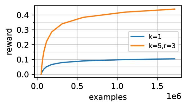
We conduct a large scale experiment using the amazon-3m dataset. Following Sen et al. (2021), we study the top-$k$ setting where $k$ actions are selected at each round. Out of the total number of actions sampled, we let $r$ denote the number of actions sampled for exploration. We apply SpannerGreedy for this dataset and consider regression functions similar to the deep models discussed before. The setting $(k=1)$ corresponds to running our algorithm unmodified, and $(k=5,r=3)$ corresponds to selecting 5 actions per round and using 3 exploration slots. Fig. 1 in Section D.4 displays the results. For $(k=1)$ the final CI is $[0.1041,0.1046]$, and for $(k=5,r=3)$ the final CI is $[0.438,0.440]$.

In the setup with $(k=5,r=3)$, our results are directly comparable to Sen et al. (2021), who evaluated a tree-based contextual bandit method on the same dataset. The best result from Sen et al. (2021) achieves roughly 0.19 reward with $(k=5,r=3)$, which we exceed by a factor of 2. This indicates that our use of embeddings provides favorable inductive bias for this problem, and underscores the broad utility of our techniques (which leverage embeddings). For $(k=5,r=3)$, our inference time on a commodity CPU with batch size 1 is 160ms per example, which is slower than the time of 7.85ms per example reported in Sen et al. (2021).

There is a long line of research on computationally efficient methods for contextual bandits with general function approximation, typically based on reduction to either cost-sensitive classification oracles (Langford and Zhang, 2007; Dudik et al., 2011; Agarwal et al., 2014) or regression oracles (Foster et al., 2018; Foster and Rakhlin, 2020; Simchi-Levi and Xu, 2021). Most of these works deal with a finite action spaces and have regret scaling with the number of actions, which is necessary without further structural assumptions (Agarwal et al., 2012). An exception is the works of Foster et al. (2020) and Xu and Zeevi (2020), both of which consider the same setting as the present paper. Both of the algorithms in these works require solving subproblems based on maximizing quadratic forms (which is NP-hard in general (Sahni, 1974)), and cannot directly take advantage of the linear optimization oracle we consider. Also related is the work of Zhang (2021), which proposes a posterior sampling-style algorithm for the setting we consider. This algorithm is not fully comparable computationally, as it requires sampling from specific posterior distribution; it is unclear whether this can be achieved in a provably efficient fashion.

The linear contextual bandit problem is a special case of our setting in which $g^{\star}(x)=\theta\in\mathbb{R}^{d}$ is constant (that is, the reward function only depends on the context through the feature map $\phi$). The most well-studied families of algorithms for this setting are UCB-style algorithms and posterior sampling. With a well-chosen prior and posterior distribution, posterior sampling can be implemented efficiently (Agrawal and Goyal, 2013), but it is unclear how to efficiently adapt this approach to accomodate general function approximation. Existing UCB-type algorithms require solving sub-problems based on maximizing quadratic forms, which is NP-hard in general (Sahni, 1974). One line of research aims to make UCB efficient by using hashing-based methods (MIPS) to approximate the maximum inner product (Yang et al., 2021; Jun et al., 2017). These methods have runtime sublinear (but still polynomial) in the number of actions.

For the problem of non-contextual linear bandits (with either stochastic or adversarial rewards), there is a long line of research on efficient algorithms that can take advantage of linear optimization oracles (Awerbuch and Kleinberg, 2008; McMahan and Blum, 2004; Dani and Hayes, 2006; Dani et al., 2008; Bubeck et al., 2012; Hazan and Karnin, 2016; Ito et al., 2019); see also work on the closely related problem of combinatorial pure exploration (Chen et al., 2017; Cao and Krishnamurthy, 2019; Katz-Samuels et al., 2020; Wagenmaker et al., 2021). In general, it is not clear how to lift these techniques to contextual bandits with linearly-structured actions and general function approximation. We also mention that optimal design has been applied in the context of linear bandits, but these algorithms are restricted to the non-contextual setting (Lattimore and Szepesvári, 2020; Lattimore et al., 2020), or to pure exploration (Soare et al., 2014; Fiez et al., 2019). The only exception we are aware of is Ruan et al. (2021), who extend these developments to linear contextual bandits (i.e., where $g^{\star}(x)=\theta$), but critically use that contexts are stochastic.

Another line of research provides efficient contextual bandit methods under specific modeling assumptions on the context space or action space that differ from the ones we consider here. Zhou et al. (2020); Xu et al. (2020); Zhang et al. (2021); Kassraie and Krause (2022) provide generalizations of the UCB algorithm and posterior sampling based on the Neural Tangent Kernel (NTK). These algorithms can be used to learn context embeddings (i.e., $g(x)$) with general function approximation, but only lead to theoretical guarantees under strong RKHS-based assumptions. For large action spaces, these algorithms typically require enumeration over actions. Majzoubi et al. (2020) consider a setting with nonparametric action spaces and design an efficient tree-based learner; their guarantees, however, scale exponentially in the dimensionality of action space. Sen et al. (2021) provide heuristically-motivated but empirically-effective tree-based algorithms for contextual bandits with large action spaces, with theoretical guarantees when the actions satisfy certain tree-structured properties. Lastly, another empirically-successful approach is the policy gradient method (e.g., Williams (1992); Bhatnagar et al. (2009); Pan et al. (2019)). On the theoretical side, policy gradient methods do not address the issue of systematic exploration, and—to our knowledge—do not lead to provable guarantees for the setting considered in our paper.

References

• Abbasi-Yadkori et al. (2011) Yasin Abbasi-Yadkori, Dávid Pál, and Csaba Szepesvári. Improved algorithms for linear stochastic bandits. In NIPS, volume 11, pages 2312–2320, 2011.
• Abe and Long (1999) Naoki Abe and Philip M Long. Associative reinforcement learning using linear probabilistic concepts. In ICML, pages 3–11. Citeseer, 1999.
• Agarwal et al. (2012) Alekh Agarwal, Miroslav Dudík, Satyen Kale, John Langford, and Robert Schapire. Contextual bandit learning with predictable rewards. In Artificial Intelligence and Statistics, pages 19–26. PMLR, 2012.
• Agarwal et al. (2014) Alekh Agarwal, Daniel Hsu, Satyen Kale, John Langford, Lihong Li, and Robert Schapire. Taming the monster: A fast and simple algorithm for contextual bandits. In International Conference on Machine Learning, pages 1638–1646. PMLR, 2014.
• Agarwal et al. (2016) Alekh Agarwal, Sarah Bird, Markus Cozowicz, Luong Hoang, John Langford, Stephen Lee, Jiaji Li, Dan Melamed, Gal Oshri, Oswaldo Ribas, Siddhartha Sen, and Aleksandrs Slivkins. Making contextual decisions with low technical debt. arXiv:1606.03966, 2016.
• Agrawal and Goyal (2013) Shipra Agrawal and Navin Goyal. Thompson sampling for contextual bandits with linear payoffs. In International Conference on Machine Learning, pages 127–135. PMLR, 2013.
• Atwood (1969) Corwin L Atwood. Optimal and efficient designs of experiments. The Annals of Mathematical Statistics, pages 1570–1602, 1969.
• Awerbuch and Kleinberg (2008) Baruch Awerbuch and Robert Kleinberg. Online linear optimization and adaptive routing. Journal of Computer and System Sciences, 74(1):97–114, 2008.
• Bergstra and Bengio (2012) James Bergstra and Yoshua Bengio. Random search for hyper-parameter optimization. Journal of machine learning research, 13(2), 2012.
• Bhatia et al. (2016) K. Bhatia, K. Dahiya, H. Jain, P. Kar, A. Mittal, Y. Prabhu, and M. Varma. The extreme classification repository: Multi-label datasets and code, 2016. URL http://manikvarma.org/downloads/XC/XMLRepository.html.
• Bhatnagar et al. (2009) Shalabh Bhatnagar, Richard S Sutton, Mohammad Ghavamzadeh, and Mark Lee. Natural Actor–Critic algorithms. Automatica, 45(11):2471–2482, 2009.
• Bietti et al. (2021) Alberto Bietti, Alekh Agarwal, and John Langford. A contextual bandit bake-off. Journal of Machine Learning Research, 22(133):1–49, 2021.
• Bubeck et al. (2012) Sébastien Bubeck, Nicolo Cesa-Bianchi, and Sham M Kakade. Towards minimax policies for online linear optimization with bandit feedback. In Conference on Learning Theory, pages 41–1. JMLR Workshop and Conference Proceedings, 2012.
• Cai et al. (2021) William Cai, Josh Grossman, Zhiyuan Jerry Lin, Hao Sheng, Johnny Tian-Zheng Wei, Joseph Jay Williams, and Sharad Goel. Bandit algorithms to personalize educational chatbots. Machine Learning, pages 1–30, 2021.
• Cao and Krishnamurthy (2019) Tongyi Cao and Akshay Krishnamurthy. Disagreement-based combinatorial pure exploration: Sample complexity bounds and an efficient algorithm. In Conference on Learning Theory, pages 558–588. PMLR, 2019.
• Cesa-Bianchi and Lugosi (2012) Nicolo Cesa-Bianchi and Gábor Lugosi. Combinatorial bandits. Journal of Computer and System Sciences, 78(5):1404–1422, 2012.
• Chen et al. (2017) Lijie Chen, Anupam Gupta, Jian Li, Mingda Qiao, and Ruosong Wang. Nearly optimal sampling algorithms for combinatorial pure exploration. In Conference on Learning Theory, pages 482–534. PMLR, 2017.
• Chernozhukov et al. (2019) Victor Chernozhukov, Mert Demirer, Greg Lewis, and Vasilis Syrgkanis. Semi-parametric efficient policy learning with continuous actions. Advances in Neural Information Processing Systems, 32:15065–15075, 2019.
• Chu et al. (2011) Wei Chu, Lihong Li, Lev Reyzin, and Robert Schapire. Contextual bandits with linear payoff functions. In Proceedings of the Fourteenth International Conference on Artificial Intelligence and Statistics, pages 208–214. JMLR Workshop and Conference Proceedings, 2011.
• Cohen et al. (2019) Michael B Cohen, Ben Cousins, Yin Tat Lee, and Xin Yang. A near-optimal algorithm for approximating the John Ellipsoid. In Conference on Learning Theory, pages 849–873. PMLR, 2019.
• Dani and Hayes (2006) Varsha Dani and Thomas P Hayes. Robbing the bandit: Less regret in online geometric optimization against an adaptive adversary. In SODA, volume 6, pages 937–943, 2006.
• Dani et al. (2008) Varsha Dani, Thomas P Hayes, and Sham M Kakade. Stochastic linear optimization under bandit feedback. Conference on Learning Theory (COLT), 2008.
• Devlin et al. (2019) Jacob Devlin, Ming-Wei Chang, Kenton Lee, and Kristina Toutanova. Bert: Pre-training of deep bidirectional transformers for language understanding. In NAACL-HLT (1), 2019.
• Dudik et al. (2011) Miroslav Dudik, Daniel Hsu, Satyen Kale, Nikos Karampatziakis, John Langford, Lev Reyzin, and Tong Zhang. Efficient optimal learning for contextual bandits. In Proceedings of the Twenty-Seventh Conference on Uncertainty in Artificial Intelligence, pages 169–178, 2011.
• Edmonds (1965) Jack Edmonds. Paths, trees, and flowers. Canadian Journal of mathematics, 17:449–467, 1965.
• Fiez et al. (2019) Tanner Fiez, Lalit Jain, Kevin G Jamieson, and Lillian Ratliff. Sequential experimental design for transductive linear bandits. Advances in neural information processing systems, 32, 2019.
• Foster and Rakhlin (2020) Dylan Foster and Alexander Rakhlin. Beyond UCB: Optimal and efficient contextual bandits with regression oracles. In International Conference on Machine Learning, pages 3199–3210. PMLR, 2020.
• Foster et al. (2018) Dylan Foster, Alekh Agarwal, Miroslav Dudik, Haipeng Luo, and Robert Schapire. Practical contextual bandits with regression oracles. In International Conference on Machine Learning, pages 1539–1548. PMLR, 2018.
• Foster et al. (2021a) Dylan Foster, Alexander Rakhlin, David Simchi-Levi, and Yunzong Xu. Instance-dependent complexity of contextual bandits and reinforcement learning: A disagreement-based perspective. In Conference on Learning Theory, pages 2059–2059. PMLR, 2021a.
• Foster and Krishnamurthy (2021) Dylan J Foster and Akshay Krishnamurthy. Efficient first-order contextual bandits: Prediction, allocation, and triangular discrimination. Advances in Neural Information Processing Systems, 34, 2021.
• Foster et al. (2020) Dylan J Foster, Claudio Gentile, Mehryar Mohri, and Julian Zimmert. Adapting to misspecification in contextual bandits. Advances in Neural Information Processing Systems, 33, 2020.
• Foster et al. (2021b) Dylan J Foster, Sham M Kakade, Jian Qian, and Alexander Rakhlin. The statistical complexity of interactive decision making. arXiv preprint arXiv:2112.13487, 2021b.
• Grötschel et al. (2012) Martin Grötschel, László Lovász, and Alexander Schrijver. Geometric algorithms and combinatorial optimization, volume 2. Springer Science & Business Media, 2012.
• Hazan and Karnin (2016) Elad Hazan and Zohar Karnin. Volumetric spanners: An efficient exploration basis for learning. The Journal of Machine Learning Research, 17(1):4062–4095, 2016.
• Hazan et al. (2007) Elad Hazan, Amit Agarwal, and Satyen Kale. Logarithmic regret algorithms for online convex optimization. Machine Learning, 69(2-3):169–192, 2007.
• Ito et al. (2019) Shinji Ito, Daisuke Hatano, Hanna Sumita, Kei Takemura, Takuro Fukunaga, Naonori Kakimura, and Ken-Ichi Kawarabayashi. Oracle-efficient algorithms for online linear optimization with bandit feedback. Advances in Neural Information Processing Systems, 32:10590–10599, 2019.
• John (1948) F John. Extremum problems with inequalities as subsidiary conditions. R. Courant Anniversary Volume, pages 187–204, 1948.
• Jun et al. (2017) Kwang-Sung Jun, Aniruddha Bhargava, Robert Nowak, and Rebecca Willett. Scalable generalized linear bandits: Online computation and hashing. Advances in Neural Information Processing Systems, 30, 2017.
• Kassraie and Krause (2022) Parnian Kassraie and Andreas Krause. Neural contextual bandits without regret. In International Conference on Artificial Intelligence and Statistics, pages 240–278. PMLR, 2022.
• Katz-Samuels et al. (2020) Julian Katz-Samuels, Lalit Jain, Kevin G Jamieson, et al. An empirical process approach to the union bound: Practical algorithms for combinatorial and linear bandits. Advances in Neural Information Processing Systems, 33, 2020.
• Kiefer and Wolfowitz (1960) Jack Kiefer and Jacob Wolfowitz. The equivalence of two extremum problems. Canadian Journal of Mathematics, 12:363–366, 1960.
• Krishnamurthy et al. (2020) Akshay Krishnamurthy, John Langford, Aleksandrs Slivkins, and Chicheng Zhang. Contextual bandits with continuous actions: Smoothing, zooming, and adapting. Journal of Machine Learning Research, 21(137):1–45, 2020.
• Langford and Zhang (2007) John Langford and Tong Zhang. The epoch-greedy algorithm for contextual multi-armed bandits. Advances in neural information processing systems, 20(1):96–1, 2007.
• Lattimore and Szepesvári (2020) Tor Lattimore and Csaba Szepesvári. Bandit algorithms. Cambridge University Press, 2020.
• Lattimore et al. (2020) Tor Lattimore, Csaba Szepesvari, and Gellert Weisz. Learning with good feature representations in bandits and in RL with a generative model. In International Conference on Machine Learning, pages 5662–5670. PMLR, 2020.
• Lebret and Collobert (2014) Rémi Lebret and Ronan Collobert. Word embeddings through Hellinger PCA. In Proceedings of the 14th Conference of the European Chapter of the Association for Computational Linguistics, pages 482–490, 2014.
• Li et al. (2010) Lihong Li, Wei Chu, John Langford, and Robert E Schapire. A contextual-bandit approach to personalized news article recommendation. In Proceedings of the 19th international conference on World wide web, pages 661–670, 2010.
• Mahabadi et al. (2019) Sepideh Mahabadi, Piotr Indyk, Shayan Oveis Gharan, and Alireza Rezaei. Composable core-sets for determinant maximization: A simple near-optimal algorithm. In International Conference on Machine Learning, pages 4254–4263. PMLR, 2019.
• Majzoubi et al. (2020) Maryam Majzoubi, Chicheng Zhang, Rajan Chari, Akshay Krishnamurthy, John Langford, and Aleksandrs Slivkins. Efficient contextual bandits with continuous actions. Advances in Neural Information Processing Systems, 33, 2020.
• McMahan and Blum (2004) H Brendan McMahan and Avrim Blum. Online geometric optimization in the bandit setting against an adaptive adversary. In International Conference on Computational Learning Theory, pages 109–123. Springer, 2004.
• Meyer (2000) Carl D Meyer. Matrix analysis and applied linear algebra, volume 71. Siam, 2000.
• Pan et al. (2019) Feiyang Pan, Qingpeng Cai, Pingzhong Tang, Fuzhen Zhuang, and Qing He. Policy gradients for contextual recommendations. In The World Wide Web Conference, pages 1421–1431, 2019.
• Reimers and Gurevych (2019) Nils Reimers and Iryna Gurevych. Sentence-BERT: Sentence embeddings using Siamese BERT-Networks. In Proceedings of the 2019 Conference on Empirical Methods in Natural Language Processing. Association for Computational Linguistics, 11 2019. URL http://arxiv.org/abs/1908.10084.
• Ruan et al. (2021) Yufei Ruan, Jiaqi Yang, and Yuan Zhou. Linear bandits with limited adaptivity and learning distributional optimal design. In Proceedings of the 53rd Annual ACM SIGACT Symposium on Theory of Computing, pages 74–87, 2021.
• Sahni (1974) Sartaj Sahni. Computationally related problems. SIAM Journal on computing, 3(4):262–279, 1974.
• Schrijver (1998) Alexander Schrijver. Theory of linear and integer programming. John Wiley & Sons, 1998.
• Sen et al. (2021) Rajat Sen, Alexander Rakhlin, Lexing Ying, Rahul Kidambi, Dean Foster, Daniel N Hill, and Inderjit S Dhillon. Top-k extreme contextual bandits with arm hierarchy. In International Conference on Machine Learning, pages 9422–9433. PMLR, 2021.
• Sherman and Morrison (1950) Jack Sherman and Winifred J Morrison. Adjustment of an inverse matrix corresponding to a change in one element of a given matrix. The Annals of Mathematical Statistics, 21(1):124–127, 1950.
• Shrivastava and Li (2014) Anshumali Shrivastava and Ping Li. Asymmetric LSH (ALSH) for sublinear time maximum inner product search (MIPS). Advances in neural information processing systems, 27, 2014.
• Simchi-Levi and Xu (2021) David Simchi-Levi and Yunzong Xu. Bypassing the monster: A faster and simpler optimal algorithm for contextual bandits under realizability. Mathematics of Operations Research, 2021.
• Singh et al. (2012) Sameer Singh, Amarnag Subramanya, Fernando Pereira, and Andrew McCallum. Wikilinks: A large-scale cross-document coreference corpus labeled via links to Wikipedia. Technical Report UM-CS-2012-015, University of Massachusetts, Amherst, 2012.
• Soare et al. (2014) Marta Soare, Alessandro Lazaric, and Rémi Munos. Best-arm identification in linear bandits. Advances in Neural Information Processing Systems, 27, 2014.
• Summa et al. (2014) Marco Di Summa, Friedrich Eisenbrand, Yuri Faenza, and Carsten Moldenhauer. On largest volume simplices and sub-determinants. In Proceedings of the twenty-sixth annual ACM-SIAM symposium on Discrete algorithms, pages 315–323. SIAM, 2014.
• Tewari and Murphy (2017) Ambuj Tewari and Susan A Murphy. From Ads to interventions: Contextual bandits in mobile health. In Mobile Health, pages 495–517. Springer, 2017.
• Vasnetsov (2018) Andrey Vasnetsov. Oneshot-wikilinks. https://www.kaggle.com/generall/oneshotwikilinks, 2018.
• Vovk (1998) Vladimir Vovk. A game of prediction with expert advice. Journal of Computer and System Sciences, 56(2):153–173, 1998.
• Wagenmaker et al. (2021) Andrew Wagenmaker, Julian Katz-Samuels, and Kevin Jamieson. Experimental design for regret minimization in linear bandits. In International Conference on Artificial Intelligence and Statistics, pages 3088–3096, 2021.
• Williams (1992) Ronald J Williams. Simple statistical gradient-following algorithms for connectionist reinforcement learning. Machine learning, 8(3):229–256, 1992.
• Xu et al. (2020) Pan Xu, Zheng Wen, Handong Zhao, and Quanquan Gu. Neural contextual bandits with deep representation and shallow exploration. arXiv preprint arXiv:2012.01780, 2020.
• Xu and Zeevi (2020) Yunbei Xu and Assaf Zeevi. Upper counterfactual confidence bounds: a new optimism principle for contextual bandits. arXiv preprint arXiv:2007.07876, 2020.
• Yang et al. (2021) Shuo Yang, Tongzheng Ren, Sanjay Shakkottai, Eric Price, Inderjit S Dhillon, and Sujay Sanghavi. Linear bandit algorithms with sublinear time complexity. arXiv preprint arXiv:2103.02729, 2021.
• Zhang (2021) Tong Zhang. Feel-good thompson sampling for contextual bandits and reinforcement learning. arXiv preprint arXiv:2110.00871, 2021.
• Zhang et al. (2021) Weitong Zhang, Dongruo Zhou, Lihong Li, and Quanquan Gu. Neural Thompson sampling. In International Conference on Learning Representation (ICLR), 2021.
• Zhou et al. (2020) Dongruo Zhou, Lihong Li, and Quanquan Gu. Neural contextual bandits with ucb-based exploration. In International Conference on Machine Learning, pages 11492–11502. PMLR, 2020.
Appendix A Proofs and Supporting Results from Section 3
This section is organized as follows. We provide supporting results in Section A.1, then give the proof of Theorem 1 in Section A.2.
A.1 Supporting Results
A.1.1 Barycentric Spanner and Optimal Design
Algorithm 5 restates an algorithm of Awerbuch and Kleinberg (2008), which efficiently computes a barycentric spanner (Definition 3) given access to a linear optimization oracle (Definition 1). Recall that, for a set 𝒮𝒜\mathcal{S}\subset\mathcal{A} of dd actions, the notation det(\macc@depthΔ\frozen@everymath\macc@group\macc@set@skewchar\macc@nested@a111(x,𝒮))\det(\macc@depth\char 1\relax\frozen@everymath{\macc@group}\macc@set@skewchar\macc@nested@a 111{}(x,\mathcal{S})) (resp. det(ϕ(x,𝒮))\det(\phi(x,\mathcal{S}))) denotes the determinant of the dd-by-dd matrix whose columns are the \macc@depthΔ\frozen@everymath\macc@group\macc@set@skewchar\macc@nested@a111\macc@depth\char 1\relax\frozen@everymath{\macc@group}\macc@set@skewchar\macc@nested@a 111{} (resp. ϕ\phi) embeddings of actions.
Algorithm 5 Approximate Barycentric Spanner (Awerbuch and Kleinberg, 2008)
0: Context x𝒳x\in\mathcal{X} and approximation factor C>1C>1.
1:for i=1,,di=1,\dots,d do
2:  Compute θd\theta\in{\mathbb{R}}^{d} representing linear function ϕ(x,a)det(ϕ(x,a1),,ϕ(x,ai1),ϕ(x,a),ei+1,,ed)\phi(x,a)\mapsto\det(\phi(x,a_{1}),\ldots,\phi(x,a_{i-1}),\phi(x,a),e_{i+1},\ldots,e_{d}).
3:  Get aiargmaxa𝒜|ϕ(x,a),θ|a_{i}\leftarrow\operatorname*{arg\,max}_{a\in\mathcal{A}}\lvert\langle\phi(x,a),\theta\rangle\rvert.
4: Construct 𝒮=(a1,,ad)\mathcal{S}=(a_{1},\ldots,a_{d}). // Initial set of actions 𝒮𝒜\mathcal{S}\subseteq\mathcal{A} such that |𝒮|=d\lvert\mathcal{S}\rvert=d and |det(ϕ(x,𝒮))|>0\lvert\det(\phi(x,\mathcal{S}))\rvert>0.
5:while not break do
6:  for i=1,,di=1,\dots,d do
7:   Compute θd\theta\in{\mathbb{R}}^{d} representing linear function ϕ(x,a)det(ϕ(x,𝒮i(a)))\phi(x,a)\mapsto\det(\phi(x,\mathcal{S}_{i}(a))), where 𝒮i(a):=(a1,,ai1,a,ai+1,,ad)\mathcal{S}_{i}(a)\vcentcolon=(a_{1},\ldots,a_{i-1},a,a_{i+1},\ldots,a_{d}).
8:   Get aargmaxa𝒜|ϕ(x,a),θ|a\leftarrow\operatorname*{arg\,max}_{a\in\mathcal{A}}\lvert\langle\phi(x,a),\theta\rangle\rvert.
9:   if |det(ϕ(x,𝒮i(a)))|C|det(ϕ(x,𝒮))|\lvert\det(\phi(x,\mathcal{S}_{i}(a)))\rvert\geq C\lvert\det(\phi(x,\mathcal{S}))\rvert then
10:    Update aiaa_{i}\leftarrow a.
11:    continue to line 5.
12:  break
13:return  CC-approximate barycentric spanner 𝒮\mathcal{S}.
Lemma 5 (Awerbuch and Kleinberg (2008)).
For any x𝒳x\in\mathcal{X}, Algorithm 5 computes a CC-approximate barycentric spanner for {ϕ(x,a):a𝒜}\{\phi(x,a):a\in\mathcal{A}\} within O(dlogCd)O(d\log_{C}d) iterations of the while-loop.
Lemma 6.
Fix any constant C>1C>1. Algorithm 5 can be implemented with runtime O(𝒯𝖮𝗉𝗍d2logd+d4logd)O(\mathcal{T}_{\mathsf{Opt}}\cdot d^{2}\log d+d^{4}\log d) and memory O(𝖮𝗉𝗍+d2)O(\mathcal{M}_{\mathsf{Opt}}+d^{2}).
Proof of Lemma 6.
We provide the computational complexity analysis starting from the while-loop (line 5-12) in the following. The computational complexity regarding the first for-loop (line 1-3) can be similarly analyzed.
• Outer loops (lines 5-6). From Lemma 5, we know that Algorithm 5 terminates within O(dlogd)O(d\log d) iterations of the while-loop (line 5). It is also clear that the for-loop (line 6) is invoked at most dd times.
• Computational complexity for lines 7-10. We discuss how to efficiently implement this part using rank-one updates. We analyze the computational complexity for each line in the following.
• Line 7. We discuss how to efficiently compute the linear function θ\theta through rank-one updates. Fix any YdY\in{\mathbb{R}}^{d}. Let Φ𝒮\Phi_{\mathcal{S}} denote the invertible (by construction) matrix whose kk-th column is ϕ(x,ak)\phi(x,a_{k}) (with ak𝒮a_{k}\in\mathcal{S}). Using the rank-one update formula for the determinant (Meyer, 2000), we have
det(ϕ(x,a1),,ϕ(x,ai1),Y,ϕ(x,ai+1),,ϕ(x,ad))\displaystyle\det(\phi(x,a_{1}),\ldots,\phi(x,a_{i-1}),Y,\phi(x,a_{i+1}),\ldots,\phi(x,a_{d}))
=det(Φ𝒮+(Yϕ(x,ai))ei)\displaystyle=\det\Big{(}\Phi_{\mathcal{S}}+\big{(}Y-\phi(x,a_{i})\big{)}e_{i}^{\top}\Big{)}
=det(Φ𝒮)(1+eiΦ𝒮1(Yϕ(x,ai)))\displaystyle=\det(\Phi_{\mathcal{S}})\cdot\Big{(}1+e_{i}^{\top}\Phi_{\mathcal{S}}^{-1}\big{(}Y-\phi(x,a_{i})\big{)}\Big{)}
=Y,det(Φ𝒮)(Φ𝒮1)ei+det(Φ𝒮)(1eiΦ𝒮1ϕ(x,ai)).\displaystyle=\big{\langle}Y,\det(\Phi_{\mathcal{S}})\cdot\left(\Phi_{\mathcal{S}}^{-1}\right)^{\top}e_{i}\big{\rangle}+\det(\Phi_{\mathcal{S}})\cdot\big{(}1-e_{i}^{\top}\Phi_{\mathcal{S}}^{-1}\phi(x,a_{i})\big{)}. (8)
We first notice that det(Φ𝒮)(1eiΦ𝒮1ϕ(x,ai))=0\det(\Phi_{\mathcal{S}})\cdot\big{(}1-e_{i}^{\top}\Phi_{\mathcal{S}}^{-1}\phi(x,a_{i})\big{)}=0 since one can take Y=0dY=0\in{\mathbb{R}}^{d}. We can then write
det(ϕ(x,a1),,ϕ(x,ai1),Y,ϕ(x,ai+1),,ϕ(x,ad))=Y,θ\displaystyle\det(\phi(x,a_{1}),\ldots,\phi(x,a_{i-1}),Y,\phi(x,a_{i+1}),\ldots,\phi(x,a_{d}))=\langle Y,\theta\rangle
where θ=det(Φ𝒮)(Φ𝒮1)ei\theta=\det(\Phi_{\mathcal{S}})\cdot\left(\Phi_{\mathcal{S}}^{-1}\right)^{\top}e_{i}. Thus, whenever det(Φ𝒮)\det(\Phi_{\mathcal{S}}) and Φ𝒮1\Phi_{\mathcal{S}}^{-1} are known, compute θ\theta takes O(d)O(d) time. The maximum memory requirement is O(d2)O(d^{2}), following from the storage of Φ𝒮1\Phi_{\mathcal{S}}^{-1}.
• Line 8. When θ\theta is computed, we can compute aa by first compute a+:=argmaxa𝒜ϕ(x,a),θa_{+}\vcentcolon=\operatorname*{arg\,max}_{a\in\mathcal{A}}\langle\phi(x,a),\theta\rangle and a:=argmaxa𝒜ϕ(x,a),θa_{-}\vcentcolon=\operatorname*{arg\,max}_{a\in\mathcal{A}}-\langle\phi(x,a),\theta\rangle and then compare the two. This process takes two oracle calls to 𝐀𝐥𝐠𝖮𝗉𝗍\mathrm{\mathbf{Alg}}_{\mathsf{Opt}}, which takes O(𝒯𝖮𝗉𝗍)O(\mathcal{T}_{\mathsf{Opt}}) time. The maximum memory requirement is O(𝖮𝗉𝗍+d)O(\mathcal{M}_{\mathsf{Opt}}+d), following from the memory requirement of 𝐀𝐥𝐠𝖮𝗉𝗍\mathrm{\mathbf{Alg}}_{\mathsf{Opt}} and the storage of θ\theta.
• Line 9. Once θ\theta and det(Φ𝒮)\det(\Phi_{\mathcal{S}}) are computed, checking the updating criteria takes O(d)O(d) time. The maximum memory requirement is O(d)O(d), following from the storage of ϕ(x,a)\phi(x,a) and θ\theta.
• Line 10. We discuss how to efficiently update det(Φ𝒮)\det(\Phi_{\mathcal{S}}) and Φ𝒮1\Phi_{\mathcal{S}}^{-1} through rank-one updates. If an update ai=aa_{i}=a is made, we can update the determinant using rank-one update (as in Eq. 8) with runtime O(d)O(d) and memory O(d2)O(d^{2}); and update the inverse matrix using the Sherman-Morrison rank-one update formula (Sherman and Morrison, 1950), i.e.,
(Φ𝒮+(ϕ(x,a)ϕ(x,ai))ei)1=Φ𝒮1Φ𝒮1(ϕ(x,a)ϕ(x,ai))eiΦ𝒮11+eiΦ𝒮1(ϕ(x,a)ϕ(x,ai)),\displaystyle\Big{(}\Phi_{\mathcal{S}}+\big{(}\phi(x,a)-\phi(x,a_{i})\big{)}e_{i}^{\top}\Big{)}^{-1}=\Phi_{\mathcal{S}}^{-1}-\frac{\Phi_{\mathcal{S}}^{-1}\big{(}\phi(x,a)-\phi(x,a_{i})\big{)}e_{i}^{\top}\Phi_{\mathcal{S}}^{-1}}{1+e_{i}\Phi_{\mathcal{S}}^{-1}\big{(}\phi(x,a)-\phi(x,a_{i})\big{)}},
which can be implemented in O(d2)O(d^{2}) time and memory. Note that the updated matrix must be invertible by construction.
Thus, using rank-one updates, the total runtime adds up to O(𝒯𝖮𝗉𝗍+d2)O(\mathcal{T}_{\mathsf{Opt}}+d^{2}) and the maximum memory requirement is O(𝖮𝗉𝗍+d2)O(\mathcal{M}_{\mathsf{Opt}}+d^{2}). We also remark that the initial matrix determinant and inverse can be computed cheaply since the first iteration of the first for-loop (i.e., line 2 with i=1i=1) is updated from the identity matrix.
To summarize, Algorithm 5 has runtime O(𝒯𝖮𝗉𝗍d2logd+d4logd)O(\mathcal{T}_{\mathsf{Opt}}\cdot d^{2}\log d+d^{4}\log d) and uses at most O(𝖮𝗉𝗍+d2)O(\mathcal{M}_{\mathsf{Opt}}+d^{2}) units of memory. ∎
The next proposition shows that a barycentric spanner implies an approximate optimal design. The result is well-known (e.g., Hazan and Karnin (2016)), but we provide a proof here for completeness.
See 2
Proof of Lemma 2.
Assume without loss of generality that 𝒵d\mathcal{Z}\subseteq{\mathbb{R}}^{d} spans d{\mathbb{R}}^{d}. By Definition 3, we know that for any z𝒵z\in\mathcal{Z}, we can represent zz as a weighted sum of elements in 𝒮\mathcal{S} with coefficients in the range [C,C][-C,C]. Let Φ𝒮d×d\Phi_{\mathcal{S}}\in{\mathbb{R}}^{d\times d} be the matrix whose columns are the vectors in 𝒮\mathcal{S}. For any z𝒵z\in\mathcal{Z}, we can find θ[C,C]d\theta\in[-C,C]^{d} such that z=Φ𝒮θz=\Phi_{\mathcal{S}}\theta. Since Φ𝒮\Phi_{\mathcal{S}} is invertible (by construction), we can write θ=Φ𝒮1z\theta=\Phi_{\mathcal{S}}^{-1}z, which implies the result via
C2dθ22=z(Φ𝒮Φ𝒮)12=1dzV(q)12.\displaystyle C^{2}\cdot d\geq\lVert\theta\rVert_{2}^{2}=\lVert z\rVert^{2}_{(\Phi_{\mathcal{S}}\Phi_{\mathcal{S}}^{\top})^{-1}}=\frac{1}{d}\cdot\lVert z\rVert^{2}_{V(q)^{-1}}.
A.1.2 Regret Decomposition
Fix any γ>0\gamma>0. We consider the following meta algorithm that utilizes the online regression oracle 𝐀𝐥𝐠𝖲𝗊\mathrm{\mathbf{Alg}}_{\mathsf{Sq}} defined in 2.
For t=1,2,,Tt=1,2,\ldots,T:
• Get context xt𝒳x_{t}\in\mathcal{X} from the environment and regression function f^tconv()\widehat{f}_{t}\in\operatorname{{conv}}(\mathcal{F}) from the online regression oracle 𝐀𝐥𝐠𝖲𝗊\mathrm{\mathbf{Alg}}_{\mathsf{Sq}}.
• Identify the distribution ptΔ(𝒜)p_{t}\in\Delta(\mathcal{A}) that solves the minimax problem 𝖽𝖾𝖼γ(;f^t,xt)\mathsf{dec}_{\gamma}(\mathcal{F};\widehat{f}_{t},x_{t}) (defined in Eq. 3) and play action atpta_{t}\sim p_{t}.
• Observe reward rtr_{t} and update regression oracle with example (xt,at,rt)(x_{t},a_{t},r_{t}).
The following result bounds the contextual bandit regret for the meta algorithm described above. The result is a variant of the regret decomposition based on the Decision-Estimation Coefficient given in Foster et al. (2021b), which generalizes Foster and Rakhlin (2020). The slight differences in constant terms are due to the difference in reward range.
Lemma 7 (Foster and Rakhlin (2020); Foster et al. (2021b)).
Suppose that 2 holds. Then probability at least 1δ1-\delta, the contextual bandit regret is upper bounded as follows:
𝐑𝐞𝐠𝖢𝖡(T)𝖽𝖾𝖼γ()T+2γ𝐑𝐞𝐠𝖲𝗊(T)+64γlog(2δ1)+8Tlog(2δ1).\displaystyle\mathrm{\mathbf{Reg}}_{\mathsf{CB}}(T)\leq\mathsf{dec}_{\gamma}(\mathcal{F})\cdot{}T+2\gamma\cdot\mathrm{\mathbf{Reg}}_{\mathsf{Sq}}(T)+64\gamma\cdot\log(2\delta^{-1})+\sqrt{8T\log(2\delta^{-1})}.
In general, identifying a distribution that exactly solves the minimax problem corresponding to the DEC may be impractical. However, if one can identify a distribution that instead certifies an upper bound \macc@depthΔ\frozen@everymath\macc@group\macc@set@skewchar\macc@nested@a111()γ\macc@depth\char 1\relax\frozen@everymath{\macc@group}\macc@set@skewchar\macc@nested@a 111{}_{\gamma}(\mathcal{F}) on the Decision-Estimation Coefficient (in the sense that 𝖽𝖾𝖼γ()\macc@depthΔ\frozen@everymath\macc@group\macc@set@skewchar\macc@nested@a111()γ\mathsf{dec}_{\gamma}(\mathcal{F})\leq\macc@depth\char 1\relax\frozen@everymath{\macc@group}\macc@set@skewchar\macc@nested@a 111{}_{\gamma}(\mathcal{F})), the regret bound in Lemma 7 continues to hold with 𝖽𝖾𝖼γ()\mathsf{dec}_{\gamma}(\mathcal{F}) replaced by \macc@depthΔ\frozen@everymath\macc@group\macc@set@skewchar\macc@nested@a111()γ\macc@depth\char 1\relax\frozen@everymath{\macc@group}\macc@set@skewchar\macc@nested@a 111{}_{\gamma}(\mathcal{F}).
A.1.3 Proof of Lemma 3
See 3
Proof of Lemma 3.
Fix a context x𝒳x\in\mathcal{X}. In our setting, where actions are linearly structured, we can equivalently write the Decision-Estimation Coefficient 𝖽𝖾𝖼γ(;f^,x)\mathsf{dec}_{\gamma}(\mathcal{F};\widehat{f},x) as
𝖽𝖾𝖼γ(𝒢;g^,x):=infpΔ(𝒜)supa𝒜supg𝒢𝔼ap[ϕ(x,a)ϕ(x,a),g(x)γ(ϕ(x,a),g(x)g^(x))2].\displaystyle\mathsf{dec}_{\gamma}(\mathcal{G};\widehat{g},x)\vcentcolon=\inf_{p\in\Delta(\mathcal{A})}\sup_{a^{\star}\in\mathcal{A}}\sup_{g^{\star}\in\mathcal{G}}{\mathbb{E}}_{a\sim p}\Big{[}\big{\langle}\phi(x,a^{\star})-\phi(x,a),g^{\star}(x)\big{\rangle}-{\gamma}\cdot\big{(}\big{\langle}\phi(x,a),g^{\star}(x)-\widehat{g}(x)\big{\rangle}\big{)}^{2}\bigg{]}. (9)
Recall that within our algorithms, g^conv(𝒢)\widehat{g}\in\operatorname{{conv}}(\mathcal{G}) is obtained from the estimator f^=fg^\widehat{f}=f_{\widehat{g}} output by 𝐀𝐥𝐠𝖲𝗊\mathrm{\mathbf{Alg}}_{\mathsf{Sq}}. We will bound the quantity in Eq. 9 uniformly for all x𝒳x\in\mathcal{X} and g^:𝒳d\widehat{g}:\mathcal{X}\to\mathbb{R}^{d} with g^1\|\widehat{g}\|\leq{}1. Recall that we assume supg𝒢,x𝒳g(x)1\sup_{g\in\mathcal{G},x\in\mathcal{X}}\|g(x)\|\leq 1.
Denote a^:=argmaxa𝒜ϕ(x,a),g^(x)\widehat{a}\vcentcolon=\operatorname*{arg\,max}_{a\in\mathcal{A}}\big{\langle}\phi(x,a),\widehat{g}(x)\big{\rangle} and a:=argmaxa𝒜ϕ(x,a),g(x)a^{\star}\vcentcolon=\operatorname*{arg\,max}_{a\in\mathcal{A}}\big{\langle}\phi(x,a),g^{\star}(x)\big{\rangle}. For any ε1\varepsilon\leq 1, let p:=εqopt+(1ε)𝕀a^p\vcentcolon=\varepsilon\cdot q^{\operatorname{{opt}}}+(1-\varepsilon)\cdot\mathbb{I}_{\widehat{a}}, where qoptΔ(𝒜)q^{\operatorname{{opt}}}\in\Delta(\mathcal{A}) is any CoptC_{\operatorname{{opt}}}-approximate optimal design for the embedding {ϕ(x,a)}a𝒜\left\{\phi(x,a)\right\}_{a\in\mathcal{A}}. We have the following decomposition.
𝔼ap[ϕ(x,a)ϕ(x,a),g(x)]\displaystyle{\mathbb{E}}_{a\sim p}\Big{[}\big{\langle}\phi(x,a^{\star})-\phi(x,a),g^{\star}(x)\big{\rangle}\Big{]} =𝔼ap[ϕ(x,a^)ϕ(x,a),g^(x)]+𝔼ap[ϕ(x,a),g^(x)g(x)]\displaystyle={\mathbb{E}}_{a\sim p}\Big{[}\big{\langle}\phi(x,\widehat{a})-\phi(x,a),\widehat{g}(x)\big{\rangle}\Big{]}+{\mathbb{E}}_{a\sim p}\Big{[}\big{\langle}\phi(x,a),\widehat{g}(x)-g^{\star}(x)\big{\rangle}\Big{]}
+(ϕ(x,a),g(x)ϕ(x,a^),g^(x)).\displaystyle\quad+\Big{(}\big{\langle}\phi(x,a^{\star}),g^{\star}(x)\big{\rangle}-\big{\langle}\phi(x,\widehat{a}),\widehat{g}(x)\big{\rangle}\Big{)}. (10)
For the first term in Eq. 10, we have
𝔼ap[ϕ(x,a^)ϕ(x,a),g^(x)]=ε𝔼aqopt[ϕ(x,a^)ϕ(x,a),g^(x)]2εsupx𝒳,a𝒜ϕ(x,a)supx𝒳g^(x)2ε.\displaystyle{\mathbb{E}}_{a\sim p}\Big{[}\big{\langle}\phi(x,\widehat{a})-\phi(x,a),\widehat{g}(x)\big{\rangle}\Big{]}=\varepsilon\cdot{\mathbb{E}}_{a\sim q^{\operatorname{{opt}}}}\Big{[}\big{\langle}\phi(x,\widehat{a})-\phi(x,a),\widehat{g}(x)\big{\rangle}\Big{]}\leq 2\varepsilon\cdot\sup_{x\in\mathcal{X},a\in\mathcal{A}}\|\phi(x,a)\|\cdot\sup_{x\in\mathcal{X}}\|\widehat{g}(x)\|\leq 2\varepsilon.
Next, since
ϕ(x,a),g^(x)g(x)γ2(ϕ(x,a),g^(x)g(x))2+12γ\displaystyle\big{\langle}\phi(x,a),\widehat{g}(x)-g^{\star}(x)\big{\rangle}\leq\frac{\gamma}{2}\cdot\big{(}\big{\langle}\phi(x,a),\widehat{g}(x)-g^{\star}(x)\big{\rangle}\big{)}^{2}+\frac{1}{2\gamma}
by AM-GM inequality, we can bound the second term in Eq. 10 by
𝔼ap[ϕ(x,a),g^(x)g(x)]γ2𝔼ap[(ϕ(x,a),g^(x)g(x))2]+12γ.\displaystyle{\mathbb{E}}_{a\sim p}\Big{[}\big{\langle}\phi(x,a),\widehat{g}(x)-g^{\star}(x)\big{\rangle}\Big{]}\leq\frac{\gamma}{2}\cdot{\mathbb{E}}_{a\sim p}\Big{[}\big{(}\big{\langle}\phi(x,a),\widehat{g}(x)-g^{\star}(x)\big{\rangle}\big{)}^{2}\Big{]}+\frac{1}{2\gamma}.
We now turn our attention to the third term. Observe that since a^\widehat{a} is optimal for g^\widehat{g}, ϕ(x,a^),g^(x)ϕ(x,a),g^(x)\big{\langle}\phi(x,\widehat{a}),\widehat{g}(x)\big{\rangle}\geq\big{\langle}\phi(x,a^{\star}),\widehat{g}(x)\big{\rangle}. As a result, defining V(qopt):=𝔼aqopt[ϕ(x,a)ϕ(x,a)]V(q^{\operatorname{{opt}}})\vcentcolon={\mathbb{E}}_{a\sim q^{\operatorname{{opt}}}}[\phi(x,a)\phi(x,a)^{\top}], we have
ϕ(x,a),g(x)ϕ(x,a^),g^(x)\displaystyle\big{\langle}\phi(x,a^{\star}),g^{\star}(x)\big{\rangle}-\big{\langle}\phi(x,\widehat{a}),\widehat{g}(x)\big{\rangle} ϕ(x,a),g(x)g^(x)\displaystyle\leq\big{\langle}\phi(x,a^{\star}),g^{\star}(x)-\widehat{g}(x)\big{\rangle}
ϕ(x,a)V(qopt)1g(x)g^(x)V(qopt)\displaystyle\leq\big{\|}\phi(x,a^{\star})\big{\|}_{V(q^{\operatorname{{opt}}})^{-1}}\cdot\big{\|}g^{\star}(x)-\widehat{g}(x)\big{\|}_{V(q^{\operatorname{{opt}}})}
=12γεϕ(x,a)V(qopt)12+γ2ε𝔼aqopt[(ϕ(x,a),g(x)g^(x))2]\displaystyle=\frac{1}{2\gamma\varepsilon}\cdot\big{\|}\phi(x,a^{\star})\big{\|}^{2}_{V(q^{\operatorname{{opt}}})^{-1}}+\frac{\gamma}{2}\cdot\varepsilon\cdot{\mathbb{E}}_{a\sim q^{\operatorname{{opt}}}}\Big{[}\big{(}\phi(x,a),g^{\star}(x)-\widehat{g}(x)\big{)}^{2}\Big{]}
Coptd2γε+γ2𝔼ap[(ϕ(x,a),g(x)g^(x))2].\displaystyle\leq\frac{C_{\operatorname{{opt}}}\cdot d}{2\gamma\varepsilon}+\frac{\gamma}{2}\cdot{\mathbb{E}}_{a\sim p}\Big{[}\big{(}\phi(x,a),g^{\star}(x)-\widehat{g}(x)\big{)}^{2}\Big{]}.
Here, the third line follows from the AM-GM inequality, and the last line follows from the (CoptC_{\operatorname{{opt}}}-approximate) optimal design property and the definition of pp.
Combining these bounds, we have
𝖽𝖾𝖼γ()=infpΔ(𝒜)supa𝒜supg𝒢𝖽𝖾𝖼γ(𝒢;g^,x)2ε+12γ+Coptd2γε.\displaystyle\mathsf{dec}_{\gamma}(\mathcal{F})=\inf_{p\in\Delta(\mathcal{A})}\sup_{a^{\star}\in\mathcal{A}}\sup_{g^{\star}\in\mathcal{G}}\mathsf{dec}_{\gamma}(\mathcal{G};\widehat{g},x)\leq 2\varepsilon+\frac{1}{2\gamma}+\frac{C_{\operatorname{{opt}}}\cdot d}{2\gamma\varepsilon}.
Since γ1\gamma\geq 1, taking ε:=Coptd/4γ1\varepsilon\vcentcolon=\sqrt{C_{\operatorname{{opt}}}\cdot d/4\gamma}\wedge 1 gives
𝖽𝖾𝖼γ()2Coptdγ+12γ3Coptdγ\displaystyle\mathsf{dec}_{\gamma}(\mathcal{F})\leq 2\sqrt{\frac{C_{\operatorname{{opt}}}\cdot d}{\gamma}}+\frac{1}{2\gamma}\leq 3\sqrt{\frac{C_{\operatorname{{opt}}}\cdot d}{\gamma}}
whenever ε<1\varepsilon<1. On the other hand, when ε=1\varepsilon=1, this bound holds trivially. ∎
A.2 Proof of Theorem 1
See 1
Proof of Theorem 1.
Consider γ1\gamma\geq 1. Combining Lemma 3 with Lemma 7, we have
𝐑𝐞𝐠𝖢𝖡(T)3TCoptdγ+2γ𝐑𝐞𝐠𝖲𝗊(T)+64γlog(2δ1)+8Tlog(2δ1).\displaystyle\mathrm{\mathbf{Reg}}_{\mathsf{CB}}(T)\leq 3T\cdot\sqrt{\frac{C_{\operatorname{{opt}}}\cdot d}{\gamma}}+2\gamma\cdot\mathrm{\mathbf{Reg}}_{\mathsf{Sq}}(T)+64\gamma\cdot\log(2\delta^{-1})+\sqrt{8T\log(2\delta^{-1})}.
The regret bound in Theorem 1 immediately follows by choosing
γ=(3TCoptd2𝐑𝐞𝐠𝖲𝗊(T)+64log(2δ1))2/31.\gamma=\left(\frac{3T\sqrt{C_{\operatorname{{opt}}}\cdot d}}{2\mathrm{\mathbf{Reg}}_{\mathsf{Sq}}(T)+64\log(2\delta^{-1})}\right)^{2/3}\vee 1.
In particular, when Algorithm 5 is invoked as a subroutine with parameter C=2C=2, Lemma 2 implies that we may take Copt4dC_{\operatorname{{opt}}}\leq{}4d.
Computational complexity. We now bound the per-round computational complexity of Algorithm 1 when Algorithm 5 is used as a subroutine to compute the approximate optimal design. Outside of the call to Algorithm 5, Algorithm 1 uses O(1)O(1) calls to 𝐀𝐥𝐠𝖲𝗊\mathrm{\mathbf{Alg}}_{\mathsf{Sq}} to obtain g^t(xt)d\widehat{g}_{t}(x_{t})\in{\mathbb{R}}^{d} and to update f^t\widehat{f}_{t}, and uses a single call to 𝐀𝐥𝐠𝖮𝗉𝗍\mathrm{\mathbf{Alg}}_{\mathsf{Opt}} to compute a^t\widehat{a}_{t}. With the optimal design qtoptq^{\operatorname{{opt}}}_{t} returned by Algorithm 5 (represented as a barycentric spanner), sampling from ptp_{t} takes at most O(d)O(d) time, since |supp(pt)|d+1\lvert\operatorname{supp}(p_{t})\rvert\leq d+1. outside of Algorithm 5 adds up to O(𝒯𝖲𝗊+𝒯𝖮𝗉𝗍+d)O(\mathcal{T}_{\mathsf{Sq}}+\mathcal{T}_{\mathsf{Opt}}+d). In terms of memory, calling 𝐀𝐥𝐠𝖲𝗊\mathrm{\mathbf{Alg}}_{\mathsf{Sq}} and 𝐀𝐥𝐠𝖮𝗉𝗍\mathrm{\mathbf{Alg}}_{\mathsf{Opt}} takes O(𝖲𝗊+𝖮𝗉𝗍)O(\mathcal{M}_{\mathsf{Sq}}+\mathcal{M}_{\mathsf{Opt}}) units, and maintaining the distribution ptp_{t} (the barycentric spanner) takes O(d)O(d) units, so the maximum memory (outside of Algorithm 5) is O(𝖲𝗊+𝖮𝗉𝗍+d)O(\mathcal{M}_{\mathsf{Sq}}+\mathcal{M}_{\mathsf{Opt}}+d). The stated results follow from combining the computational complexities analyzed in Lemma 6. ∎
Appendix B Proofs and Supporting Results from Section 4.1
In this section we provide supporting results concerning Algorithm 2 (Section B.1), and then give the proof of Theorem 2 (Section B.2).
B.1 Supporting Results
Lemma 8.
In Algorithm 2 (Eq. (6)), there exists a unique choice of λ>0\lambda>0 such that a𝒜pt(a)=1\sum_{a\in\mathcal{A}}p_{t}(a)=1, and its value lies in [12,1][\frac{1}{2},1].
Proof of Lemma 8.
Define h(λ):=asupp(qt)qt(a)λ+η(f^t(xt,a^t)f^t(xt,a))h(\lambda)\vcentcolon=\sum_{a\in\operatorname{supp}(q_{t})}\frac{q_{t}(a)}{\lambda+\eta(\widehat{f}_{t}(x_{t},\widehat{a}_{t})-\widehat{f}_{t}(x_{t},a))}. We first notice that h(λ)h(\lambda) is continuous and strictly decreasing over (0,)(0,\infty). We further have
h(1/2)\displaystyle h({1}/{2}) qt(a^t)1/2+η(f^t(xt,a^t)f^t(xt,a^t))1/21/2=1;\displaystyle\geq\frac{q_{t}(\widehat{a}_{t})}{{1}/{2}+\eta(\widehat{f}_{t}(x_{t},\widehat{a}_{t})-\widehat{f}_{t}(x_{t},\widehat{a}_{t}))}\geq\frac{1/2}{1/2}=1;
and
h(1)asupp(qt)qt(a)=12+12asupp(qtopt)qtopt(a)=1.\displaystyle h(1)\leq\sum_{a\in\operatorname{supp}(q_{t})}q_{t}(a)=\frac{1}{2}+\frac{1}{2}\sum_{a\in\operatorname{supp}(q^{\operatorname{{opt}}}_{t})}q^{\operatorname{{opt}}}_{t}(a)=1.
As a result, there exists a unique normalization constant λ[12,1]\lambda^{\star}\in[\frac{1}{2},1] such that h(λ)=1h(\lambda^{\star})=1. ∎
See 4
Proof of Lemma 4.
As in the proof of Lemma 3, we use the linear structure of the action space to rewrite the Decision-Estimation Coefficient 𝖽𝖾𝖼γ(;f^,x)\mathsf{dec}_{\gamma}(\mathcal{F};\widehat{f},x) as
𝖽𝖾𝖼γ(𝒢;g^,x):=infpΔ(𝒜)supa𝒜supg𝒢𝔼ap[ϕ(x,a)ϕ(x,a),g(x)γ(ϕ(x,a),g(x)g^(x))2],\displaystyle\mathsf{dec}_{\gamma}(\mathcal{G};\widehat{g},x)\vcentcolon=\inf_{p\in\Delta(\mathcal{A})}\sup_{a^{\star}\in\mathcal{A}}\sup_{g^{\star}\in\mathcal{G}}{\mathbb{E}}_{a\sim p}\Big{[}\big{\langle}\phi(x,a^{\star})-\phi(x,a),g^{\star}(x)\big{\rangle}-{\gamma}\cdot\big{(}\big{\langle}\phi(x,a),g^{\star}(x)-\widehat{g}(x)\big{\rangle}\big{)}^{2}\bigg{]},
Where g^\widehat{g} is such that f^=fg^\widehat{f}=f_{\widehat{g}}. We will bound the quantity above uniformly for all x𝒳x\in\mathcal{X} and g^:𝒳d\widehat{g}:\mathcal{X}\to\mathbb{R}^{d}.
Denote a^:=argmaxa𝒜ϕ(x,a),g^(x)\widehat{a}\vcentcolon=\operatorname*{arg\,max}_{a\in\mathcal{A}}\big{\langle}\phi(x,a),\widehat{g}(x)\big{\rangle}, a:=argmaxa𝒜ϕ(x,a),g(x)a^{\star}\vcentcolon=\operatorname*{arg\,max}_{a\in\mathcal{A}}\big{\langle}\phi(x,a),g^{\star}(x)\big{\rangle} and qoptΔ(𝒜)q^{\operatorname{{opt}}}\in\Delta(\mathcal{A}) be a CoptC_{\operatorname{{opt}}}-approximate optimal design with respect to the reweighted embedding \macc@depthΔ\frozen@everymath\macc@group\macc@set@skewchar\macc@nested@a111(x,)\macc@depth\char 1\relax\frozen@everymath{\macc@group}\macc@set@skewchar\macc@nested@a 111{}(x,\cdot)). We use the setting η=γCoptd\eta=\frac{\gamma}{C_{\operatorname{{opt}}}\cdot d} throughout the proof. Recall that for the sampling distribution in Algorithm 2, we set q:=12qopt+12𝕀a^q\vcentcolon=\frac{1}{2}q^{\operatorname{{opt}}}+\frac{1}{2}\mathbb{I}_{\widehat{a}} and define
p(a)=q(a)λ+γCoptd(ϕ(x,a^)ϕ(x,a),g^(x)),\displaystyle p(a)=\frac{q(a)}{\lambda+\frac{\gamma}{C_{\operatorname{{opt}}}\cdot d}\left(\big{\langle}\phi(x,\widehat{a})-\phi(x,a),\widehat{g}(x)\big{\rangle}\right)}, (11)
where λ[12,1]\lambda\in[\frac{1}{2},1] is a normalization constant (cf. Lemma 8).
We decompose the regret of the distribution pp in Eq. 11 as
+ϕ(x,a),g(x)g^(x)+ϕ(x,a)ϕ(x,a^),g^(x).\displaystyle\quad+\big{\langle}\phi(x,a^{\star}),g^{\star}(x)-\widehat{g}(x)\big{\rangle}+\big{\langle}\phi(x,a^{\star})-\phi(x,\widehat{a}),\widehat{g}(x)\big{\rangle}. (12)
Writing out the expectation, the first term in Eq. 12 is upper bounded as follows.
𝔼ap[ϕ(x,a^)ϕ(x,a),g^(x)]\displaystyle{\mathbb{E}}_{a\sim p}\Big{[}\big{\langle}\phi(x,\widehat{a})-\phi(x,a),\widehat{g}(x)\big{\rangle}\Big{]} =asupp(qopt){a^}p(a)ϕ(x,a^)ϕ(x,a),g^(x)\displaystyle=\sum_{a\in\operatorname{supp}(q^{\operatorname{{opt}}})\cup\{\widehat{a}\}}p(a)\cdot\big{\langle}\phi(x,\widehat{a})-\phi(x,a),\widehat{g}(x)\big{\rangle}
<asupp(qopt)qopt(a)/2γCoptd(ϕ(x,a^)ϕ(x,a),g^(x))ϕ(x,a^)ϕ(x,a),g^(x)\displaystyle<\sum_{a\in\operatorname{supp}(q^{\operatorname{{opt}}})}\frac{q^{\operatorname{{opt}}}(a)/2}{\frac{\gamma}{C_{\operatorname{{opt}}}\cdot d}\left(\big{\langle}\phi(x,\widehat{a})-\phi(x,a),\widehat{g}(x)\big{\rangle}\right)}\cdot\big{\langle}\phi(x,\widehat{a})-\phi(x,a),\widehat{g}(x)\big{\rangle}
Coptd2γ,\displaystyle\leq\frac{C_{\operatorname{{opt}}}\cdot d}{2\gamma},
where we use that λ>0\lambda>0 in the second inequality (with the convention that 00=0\frac{0}{0}=0).
The second term in Eq. 12 can be upper bounded as in the proof of Lemma 3, by applying the AM-GM inequality:
𝔼ap[ϕ(x,a),g(x)g^(x)]γ2𝔼ap[(ϕ(x,a),g^(x)g(x))2]+12γ.\displaystyle{\mathbb{E}}_{a\sim p}\Big{[}\big{\langle}\phi(x,a),g^{\star}(x)-\widehat{g}(x)\big{\rangle}\Big{]}\leq\frac{\gamma}{2}\cdot{\mathbb{E}}_{a\sim p}\Big{[}\big{(}\big{\langle}\phi(x,a),\widehat{g}(x)-g^{\star}(x)\big{\rangle}\big{)}^{2}\Big{]}+\frac{1}{2\gamma}.
The third term in Eq. 12 is the most involved. To begin, we define V(p):=𝔼ap[ϕ(x,a)ϕ(x,a)]V(p)\vcentcolon={\mathbb{E}}_{a\sim p}[\phi(x,a)\phi(x,a)^{\top}] and apply the following standard bound:
ϕ(x,a),g^(x)g(x)\displaystyle\big{\langle}\phi(x,a^{\star}),\widehat{g}(x)-g^{\star}(x)\big{\rangle} ϕ(x,a)V(p)1g(x)g^(x)V(p)\displaystyle\leq\big{\|}\phi(x,a^{\star})\big{\|}_{V(p)^{-1}}\cdot\big{\|}g^{\star}(x)-\widehat{g}(x)\big{\|}_{V(p)}
12γϕ(x,a)V(p)12+γ2g(x)g^(x)V(p)2\displaystyle\leq\frac{1}{2\gamma}\cdot\big{\|}\phi(x,a^{\star})\big{\|}^{2}_{V(p)^{-1}}+\frac{\gamma}{2}\cdot\big{\|}g^{\star}(x)-\widehat{g}(x)\big{\|}^{2}_{V(p)}
=12γϕ(x,a)V(p)12+γ2𝔼ap[(ϕ(x,a),g(x)g^(x))2],\displaystyle=\frac{1}{2\gamma}\cdot\big{\|}\phi(x,a^{\star})\big{\|}^{2}_{V(p)^{-1}}+\frac{\gamma}{2}\cdot{\mathbb{E}}_{a\sim p}\Big{[}\big{(}\phi(x,a),g^{\star}(x)-\widehat{g}(x)\big{)}^{2}\Big{]}, (13)
where the second line follows from the AM-GM inequality. The second term in Eq. 13 matches the bound we desired, so it remains to bound the first term. Let qˇopt{\check{q}}^{\operatorname{{opt}}} be the following sub-probability measure:
qˇopt(a):=qopt(a)/2λ+γCoptd(ϕ(x,a^)ϕ(x,a),g^(x)),\displaystyle{\check{q}}^{\operatorname{{opt}}}(a)\vcentcolon=\frac{q^{\operatorname{{opt}}}(a)/2}{\lambda+\frac{\gamma}{C_{\operatorname{{opt}}}\cdot d}\left(\big{\langle}\phi(x,\widehat{a})-\phi(x,a),\widehat{g}(x)\big{\rangle}\right)},
and let V(qˇopt):=𝔼aqˇopt[ϕ(x,a)ϕ(x,a)]V({\check{q}}^{\operatorname{{opt}}})\vcentcolon={\mathbb{E}}_{a\sim{\check{q}}^{\operatorname{{opt}}}}[\phi(x,a)\phi(x,a)^{\top}]. We clearly have V(p)V(qˇopt)V(p)\succeq V({\check{q}}^{\operatorname{{opt}}}) from the definition of pp (cf. Eq. 11). We observe that
V(qˇopt)\displaystyle V({\check{q}}^{\operatorname{{opt}}}) =asupp(qˇopt)qˇopt(a)ϕ(x,a)ϕ(x,a)\displaystyle=\sum_{a\in\operatorname{supp}({\check{q}}^{\operatorname{{opt}}})}{\check{q}}^{\operatorname{{opt}}}(a)\phi(x,a)\phi(x,a)^{\top}
=12asupp(qopt)qopt(a)\macc@depthΔ\frozen@everymath\macc@group\macc@set@skewchar\macc@nested@a111(x,a)\macc@depthΔ\frozen@everymath\macc@group\macc@set@skewchar\macc@nested@a111(x,a)1+γCoptd(ϕ(x,a^)ϕ(x,a),g^(x))λ+γCoptd(ϕ(x,a^)ϕ(x,a),g^(x))\displaystyle=\frac{1}{2}\cdot\sum_{a\in\operatorname{supp}(q^{\operatorname{{opt}}})}q^{\operatorname{{opt}}}(a)\macc@depth\char 1\relax\frozen@everymath{\macc@group}\macc@set@skewchar\macc@nested@a 111{}(x,a)\macc@depth\char 1\relax\frozen@everymath{\macc@group}\macc@set@skewchar\macc@nested@a 111{}(x,a)^{\top}\cdot\frac{1+\frac{\gamma}{C_{\operatorname{{opt}}}\cdot d}\left(\big{\langle}\phi(x,\widehat{a})-\phi(x,a),\widehat{g}(x)\big{\rangle}\right)}{\lambda+\frac{\gamma}{C_{\operatorname{{opt}}}\cdot d}\left(\big{\langle}\phi(x,\widehat{a})-\phi(x,a),\widehat{g}(x)\big{\rangle}\right)}
12asupp(qopt)qopt(a)\macc@depthΔ\frozen@everymath\macc@group\macc@set@skewchar\macc@nested@a111(x,a)\macc@depthΔ\frozen@everymath\macc@group\macc@set@skewchar\macc@nested@a111(x,a)=:12\macc@depthΔ\frozen@everymath\macc@group\macc@set@skewchar\macc@nested@a111V(qopt),\displaystyle\succeq\frac{1}{2}\cdot\sum_{a\in\operatorname{supp}(q^{\operatorname{{opt}}})}q^{\operatorname{{opt}}}(a)\macc@depth\char 1\relax\frozen@everymath{\macc@group}\macc@set@skewchar\macc@nested@a 111{}(x,a)\macc@depth\char 1\relax\frozen@everymath{\macc@group}\macc@set@skewchar\macc@nested@a 111{}(x,a)^{\top}=\vcentcolon\frac{1}{2}\macc@depth\char 1\relax\frozen@everymath{\macc@group}\macc@set@skewchar\macc@nested@a 111{V}(q^{\operatorname{{opt}}}),
where the last line uses that λ1\lambda\leq 1. Since \macc@depthΔ\frozen@everymath\macc@group\macc@set@skewchar\macc@nested@a111V(qopt)\macc@depth\char 1\relax\frozen@everymath{\macc@group}\macc@set@skewchar\macc@nested@a 111{V}(q^{\operatorname{{opt}}}) is positive-definite by construction, we have that V(p)1V(qˇopt)12\macc@depthΔ\frozen@everymath\macc@group\macc@set@skewchar\macc@nested@a111V(qopt)1V(p)^{-1}\preceq V({\check{q}}^{\operatorname{{opt}}})^{-1}\preceq 2\cdot\macc@depth\char 1\relax\frozen@everymath{\macc@group}\macc@set@skewchar\macc@nested@a 111{V}(q^{\operatorname{{opt}}})^{-1}. As a result,
12γϕ(x,a)V(p)12\displaystyle\frac{1}{2\gamma}\cdot\big{\|}\phi(x,a^{\star})\big{\|}^{2}_{V(p)^{-1}} 1γϕ(x,a)\macc@depthΔ\frozen@everymath\macc@group\macc@set@skewchar\macc@nested@a111V(qopt)12\displaystyle\leq\frac{1}{\gamma}\cdot\big{\|}\phi(x,a^{\star})\big{\|}^{2}_{\macc@depth\char 1\relax\frozen@everymath{\macc@group}\macc@set@skewchar\macc@nested@a 111{V}(q^{\operatorname{{opt}}})^{-1}}
=1+γCoptd(ϕ(x,a^)ϕ(x,a),g^(x))γ\macc@depthΔ\frozen@everymath\macc@group\macc@set@skewchar\macc@nested@a111(x,a)\macc@depthΔ\frozen@everymath\macc@group\macc@set@skewchar\macc@nested@a111V(qopt)12\displaystyle=\frac{1+\frac{\gamma}{C_{\operatorname{{opt}}}\cdot d}\big{(}\big{\langle}\phi(x,\widehat{a})-\phi(x,a^{\star}),\widehat{g}(x)\big{\rangle}\big{)}}{\gamma}\cdot\big{\|}\macc@depth\char 1\relax\frozen@everymath{\macc@group}\macc@set@skewchar\macc@nested@a 111{}(x,a^{\star})\big{\|}^{2}_{\macc@depth\char 1\relax\frozen@everymath{\macc@group}\macc@set@skewchar\macc@nested@a 111{V}(q^{\operatorname{{opt}}})^{-1}}
Coptdγ+ϕ(x,a^)ϕ(x,a),g^(x),\displaystyle\leq\frac{C_{\operatorname{{opt}}}\cdot d}{\gamma}+\big{\langle}\phi(x,\widehat{a})-\phi(x,a^{\star}),\widehat{g}(x)\big{\rangle}, (14)
where the last line uses that \macc@depthΔ\frozen@everymath\macc@group\macc@set@skewchar\macc@nested@a111(x,a)\macc@depthΔ\frozen@everymath\macc@group\macc@set@skewchar\macc@nested@a111V(qopt)12Coptd\big{\|}\macc@depth\char 1\relax\frozen@everymath{\macc@group}\macc@set@skewchar\macc@nested@a 111{}(x,a^{\star})\big{\|}^{2}_{\macc@depth\char 1\relax\frozen@everymath{\macc@group}\macc@set@skewchar\macc@nested@a 111{V}(q^{\operatorname{{opt}}})^{-1}}\leq C_{\operatorname{{opt}}}\cdot d, since qoptq^{\operatorname{{opt}}} is a CoptC_{\operatorname{{opt}}}-approximate optimal design for the set {\macc@depthΔ\frozen@everymath\macc@group\macc@set@skewchar\macc@nested@a111(x,a)}a𝒜\left\{\macc@depth\char 1\relax\frozen@everymath{\macc@group}\macc@set@skewchar\macc@nested@a 111{}(x,a)\right\}_{a\in\mathcal{A}}. Finally, we observe that the second term in Eq. 14 is cancelled out by the forth term in Eq. 12.
Summarizing the bounds on the terms in Eq. 12 leads to:
𝖽𝖾𝖼γ()=infpΔ(𝒜)supa𝒜supg𝒢𝖽𝖾𝖼γ(𝒢;g^,x)Coptd2γ+12γ+Coptdγ2Coptdγ.\displaystyle\mathsf{dec}_{\gamma}(\mathcal{F})=\inf_{p\in\Delta(\mathcal{A})}\sup_{a^{\star}\in\mathcal{A}}\sup_{g^{\star}\in\mathcal{G}}\mathsf{dec}_{\gamma}(\mathcal{G};\widehat{g},x)\leq\frac{C_{\operatorname{{opt}}}\cdot d}{2\gamma}+\frac{1}{2\gamma}+\frac{C_{\operatorname{{opt}}}\cdot d}{\gamma}\leq\frac{2\,C_{\operatorname{{opt}}}\cdot d}{\gamma}.
B.2 Proof of Theorem 2
Proof.
Combining Lemma 4 with Lemma 7, we have
𝐑𝐞𝐠𝖢𝖡(T)2TCoptdγ+2γ𝐑𝐞𝐠𝖲𝗊(T)+64γlog(2δ1)+8Tlog(2δ1).\displaystyle\mathrm{\mathbf{Reg}}_{\mathsf{CB}}(T)\leq 2T\cdot{\frac{C_{\operatorname{{opt}}}\cdot d}{\gamma}}+2\gamma\cdot\mathrm{\mathbf{Reg}}_{\mathsf{Sq}}(T)+64\gamma\cdot\log(2\delta^{-1})+\sqrt{8T\log(2\delta^{-1})}.
The theorem follows by choosing
γ=(CoptdT𝐑𝐞𝐠𝖲𝗊(T)+32log(2δ1))1/2.\displaystyle\gamma=\left(\frac{C_{\operatorname{{opt}}}\cdot d\,T}{\mathrm{\mathbf{Reg}}_{\mathsf{Sq}}(T)+32\log(2\delta^{-1})}\right)^{1/2}.
In particular, when Algorithm 3 is invoked as the subroutine with parameter C=2C=2, we may take Copt=4dC_{\operatorname{{opt}}}=4d.
Computational complexity. We now discuss the per-round computational complexity of Algorithm 2. We analyze a variant of the sampling rule specified in Section D.2 that does not require computation of the normalization constant. Outside of the runtime and memory requirements required to compute the barycentric spanner using Algorithm 3, which are stated in Theorem 3, Algorithm 2 uses O(1)O(1) calls to the oracle 𝐀𝐥𝐠𝖲𝗊\mathrm{\mathbf{Alg}}_{\mathsf{Sq}} to obtain g^t(xt)d\widehat{g}_{t}(x_{t})\in{\mathbb{R}}^{d} and update f^t\widehat{f}_{t}, and uses a single call to 𝐀𝐥𝐠𝖮𝗉𝗍\mathrm{\mathbf{Alg}}_{\mathsf{Opt}} to compute a^t\widehat{a}_{t}. With g^t(xt)\widehat{g}_{t}(x_{t}) and a^t\widehat{a}_{t}, we can compute f^t(xt,a^t)f^t(xt,a)=ϕ(xt,a^t)ϕ(xt,a),g^t(xt)\widehat{f}_{t}(x_{t},\widehat{a}_{t})-\widehat{f}_{t}(x_{t},a)=\langle\phi(x_{t},\widehat{a}_{t})-\phi(x_{t},a),\widehat{g}_{t}(x_{t})\rangle in O(d)O(d) time for any a𝒜a\in\mathcal{A}; thus, with the optimal design qtoptq^{\operatorname{{opt}}}_{t} returned by Algorithm 3 (represented as a barycentric spanner), we can construct the sampling distribution ptp_{t} in O(d2)O(d^{2}) time. Sampling from ptp_{t} takes O(d)O(d) time since |supp(pt)|d+1\lvert\operatorname{supp}(p_{t})\rvert\leq d+1. This adds up to runtime O(𝒯𝖲𝗊+𝒯𝖮𝗉𝗍+d2)O(\mathcal{T}_{\mathsf{Sq}}+\mathcal{T}_{\mathsf{Opt}}+d^{2}). In terms of memory, calling 𝐀𝐥𝐠𝖲𝗊\mathrm{\mathbf{Alg}}_{\mathsf{Sq}} and 𝐀𝐥𝐠𝖮𝗉𝗍\mathrm{\mathbf{Alg}}_{\mathsf{Opt}} takes O(𝖲𝗊+𝖮𝗉𝗍)O(\mathcal{M}_{\mathsf{Sq}}+\mathcal{M}_{\mathsf{Opt}}) units, and maintaining the distribution ptp_{t} (the barycentric spanner) takes O(d)O(d) units, so the maximum memory (outside of Algorithm 3) is O(𝖲𝗊+𝖮𝗉𝗍+d)O(\mathcal{M}_{\mathsf{Sq}}+\mathcal{M}_{\mathsf{Opt}}+d). The stated results follow from combining the computational complexities analyzed in Theorem 3 , together with the choice of γ\gamma described above. ∎
Appendix C Proofs and Supporting Results from Section 4.2
This section of the appendix is dedicated to the analysis of Algorithm 3, and organized as follows.
Throughout this section of the appendix, we assume that the context x𝒳x\in\mathcal{X} and estimator g^:𝒳d\widehat{g}:\mathcal{X}\to\mathbb{R}^{d}—which are arguments to Algorithm 3 and Algorithm 4—are fixed.
C.1 Analysis of Algorithm 4 (Linear Optimization Oracle for Reweighted Embeddings)
A first step is to construct an (approximate) argmax oracle (after taking absolute value) with respect to the reweighted embedding \macc@depthΔ\frozen@everymath\macc@group\macc@set@skewchar\macc@nested@a111\macc@depth\char 1\relax\frozen@everymath{\macc@group}\macc@set@skewchar\macc@nested@a 111{}. Recall that the goal of Algorithm 4 is to implement a linear optimization oracle for the reweighted embeddings constructed by Algorithm 3. That is, for any θd\theta\in\mathbb{R}^{d}, we would like to compute an action that (approximately) solves
argmaxa𝒜|\macc@depthΔ\frozen@everymath\macc@group\macc@set@skewchar\macc@nested@a111(x,a),θ|=argmaxa𝒜\macc@depthΔ\frozen@everymath\macc@group\macc@set@skewchar\macc@nested@a111(x,a),θ2.\displaystyle\operatorname*{arg\,max}_{a\in\mathcal{A}}\big{\lvert}\big{\langle}\macc@depth\char 1\relax\frozen@everymath{\macc@group}\macc@set@skewchar\macc@nested@a 111{}(x,a),\theta\big{\rangle}\big{\rvert}=\operatorname*{arg\,max}_{a\in\mathcal{A}}{\big{\langle}\macc@depth\char 1\relax\frozen@everymath{\macc@group}\macc@set@skewchar\macc@nested@a 111{}(x,a),\theta\big{\rangle}}^{2}.
Define
ι(a):=\macc@depthΔ\frozen@everymath\macc@group\macc@set@skewchar\macc@nested@a111(x,a),θ2,anda:=argmaxa𝒜ι(a).\iota(a)\vcentcolon=\langle\macc@depth\char 1\relax\frozen@everymath{\macc@group}\macc@set@skewchar\macc@nested@a 111{}(x,a),\theta\rangle^{2},\quad\text{and}\quad a^{\star}\vcentcolon=\operatorname*{arg\,max}_{a\in\mathcal{A}}\iota(a). (15)
The main result of this section, Theorem 4, shows that Algorithm 4 identifies an action that achieves the maximum value in Eq. 15 up to a multiplicative constant.
Theorem 4.
Fix any η>0\eta>{}0, r(0,1)r\in(0,1). Suppose ζι(a)1\zeta\leq\sqrt{\iota(a^{\star})}\leq 1 for some ζ>0\zeta>0. Then Algorithm 4 identifies an action aˇ\check{a} such that ι(aˇ)22ι(a)\sqrt{\iota(\check{a})}\geq\frac{\sqrt{2}}{2}\cdot{}\sqrt{\iota(a^{\star})}, and does so with runtime O((𝒯𝖮𝗉𝗍+d)log(eηζ))O((\mathcal{T}_{\mathsf{Opt}}+d)\cdot\log(e\vee\frac{\eta}{\zeta})) and maximum memory O(𝖮𝗉𝗍+log(eηζ)+d)O(\mathcal{M}_{\mathsf{Opt}}+\log(e\vee\frac{\eta}{\zeta})+d).
Proof of Theorem 4.
Recall from Eq. 5 that we have
\macc@depthΔ\frozen@everymath\macc@group\macc@set@skewchar\macc@nested@a111(x,a),θ2=(ϕ(x,a),θ1+ηϕ(x,a^)ϕ(x,a),g^(x))2=ϕ(x,a),θ21+ηϕ(x,a^)ϕ(x,a),g^(x),\displaystyle{\big{\langle}\macc@depth\char 1\relax\frozen@everymath{\macc@group}\macc@set@skewchar\macc@nested@a 111{}(x,a),\theta\big{\rangle}}^{2}=\left(\frac{{\big{\langle}\phi(x,a),\theta\big{\rangle}}}{\sqrt{1+\eta\big{\langle}\phi(x,\widehat{a})-\phi(x,a),\widehat{g}(x)\big{\rangle}}}\right)^{2}=\frac{{\big{\langle}\phi(x,a),\theta\big{\rangle}}^{2}}{{1+\eta\big{\langle}\phi(x,\widehat{a})-\phi(x,a),\widehat{g}(x)\big{\rangle}}},
where a^:=argmaxa𝒜ϕ(x,a),g^(x)\widehat{a}\vcentcolon=\operatorname*{arg\,max}_{a\in\mathcal{A}}\left\langle\phi(x,a),\widehat{g}(x)\right\rangle; note that the denominator is at least 11. To proceed, we use that for any XX\in\mathbb{R} and Y2>0Y^{2}>0, we have
X2Y2=supε{2εXε2Y2}.\displaystyle\frac{X^{2}}{Y^{2}}=\sup_{\varepsilon\in{\mathbb{R}}}\left\{2\varepsilon X-\varepsilon^{2}Y^{2}\right\}.
Taking X=ϕ(x,a),θX=\big{\langle}\phi(x,a),\theta\big{\rangle} and Y2=1+ηϕ(x,a^)ϕ(x,a),g^(x)Y^{2}={1+\eta\big{\langle}\phi(x,\widehat{a})-\phi(x,a),\widehat{g}(x)\big{\rangle}} above, we can write
\macc@depthΔ\frozen@everymath\macc@group\macc@set@skewchar\macc@nested@a111(x,a),θ2\displaystyle{\big{\langle}\macc@depth\char 1\relax\frozen@everymath{\macc@group}\macc@set@skewchar\macc@nested@a 111{}(x,a),\theta\big{\rangle}}^{2} =ϕ(x,a),θ21+ηϕ(x,a^)ϕ(x,a),g^(x)\displaystyle=\frac{{\big{\langle}\phi(x,a),\theta\big{\rangle}}^{2}}{{1+\eta\big{\langle}\phi(x,\widehat{a})-\phi(x,a),\widehat{g}(x)\big{\rangle}}}
=supε{2εϕ(x,a),θε2(1+ηϕ(x,a^)ϕ(x,a),g^(x))}\displaystyle=\sup_{\varepsilon\in\mathbb{R}}\Big{\{}2\varepsilon\big{\langle}\phi(x,a),\theta\big{\rangle}-\varepsilon^{2}\cdot\big{(}{1+\eta\big{\langle}\phi(x,\widehat{a})-\phi(x,a),\widehat{g}(x)\big{\rangle}}\big{)}\Big{\}} (16)
=supε{ϕ(x,a),2εθ+ηε2g^(x)ε2ηε2ϕ(x,a^),g^(x)}.\displaystyle=\sup_{\varepsilon\in\mathbb{R}}\Big{\{}\big{\langle}\phi(x,a),2\varepsilon\theta+\eta\varepsilon^{2}\widehat{g}(x)\big{\rangle}-\varepsilon^{2}-\eta\varepsilon^{2}\big{\langle}\phi(x,\widehat{a}),\widehat{g}(x)\big{\rangle}\Big{\}}. (17)
The key property of this representation is that for any fixed ε\varepsilon\in\mathbb{R}, Eq. 17 is a linear function of the unweighted embedding ϕ\phi, and hence can be optimized using 𝐀𝐥𝐠𝖮𝗉𝗍\mathrm{\mathbf{Alg}}_{\mathsf{Opt}}. In particular, for any fixed ε\varepsilon\in\mathbb{R}, consider the following linear optimization problem, which can be solved by calling 𝐀𝐥𝐠𝖮𝗉𝗍\mathrm{\mathbf{Alg}}_{\mathsf{Opt}}:
argmaxa𝒜{2εϕ(x,a),θε2(1+ηϕ(x,a^)ϕ(x,a),g^(x))}=:argmaxa𝒜W(a;ε).\displaystyle\operatorname*{arg\,max}_{a\in\mathcal{A}}\Big{\{}2\varepsilon\big{\langle}\phi(x,a),\theta\big{\rangle}-\varepsilon^{2}\cdot\big{(}{1+\eta\big{\langle}\phi(x,\widehat{a})-\phi(x,a),\widehat{g}(x)\big{\rangle}}\big{)}\Big{\}}=\vcentcolon\operatorname*{arg\,max}_{a\in\mathcal{A}}W(a;\varepsilon). (18)
ε:=ϕ(x,a),θ1+ηϕ(x,a^)ϕ(x,a),g^(x).\displaystyle\varepsilon^{\star}\vcentcolon=\frac{\langle\phi(x,a^{\star}),\theta\rangle}{{1+\eta\langle\phi(x,\widehat{a})-\phi(x,a^{\star}),\widehat{g}(x)\rangle}}. (19)
If ε\varepsilon^{\star} was known (which is not the case, since aa^{\star} is unknown), we could set ε=ε\varepsilon=\varepsilon^{\star} in Eq. 18 and compute an action \macc@depthΔ\frozen@everymath\macc@group\macc@set@skewchar\macc@nested@a111a:=argmaxa𝒜W(a;ε)\macc@depth\char 1\relax\frozen@everymath{\macc@group}\macc@set@skewchar\macc@nested@a 111{a}\vcentcolon=\operatorname*{arg\,max}_{a\in\mathcal{A}}W(a;\varepsilon^{\star}) using a single oracle call. We would then have ι(\macc@depthΔ\frozen@everymath\macc@group\macc@set@skewchar\macc@nested@a111a)W(\macc@depthΔ\frozen@everymath\macc@group\macc@set@skewchar\macc@nested@a111a;ε)W(a;ε)=ι(a)\iota(\macc@depth\char 1\relax\frozen@everymath{\macc@group}\macc@set@skewchar\macc@nested@a 111{a})\geq W(\macc@depth\char 1\relax\frozen@everymath{\macc@group}\macc@set@skewchar\macc@nested@a 111{a};\varepsilon^{\star})\geq W(a^{\star};\varepsilon^{\star})=\iota(a^{\star}), which follows because ε\varepsilon^{\star} is the maximizer in Eq. 16 for a=aa=a^{\star}.
To get around the fact that ε\varepsilon^{\star} is unknown, Algorithm 4 performs a grid search over possible values of ε\varepsilon. To show that the procedure succeeds, we begin by bounding the range of ε\varepsilon^{\star}. With some rewriting, we have