Contextual Pandora’s Box

Alexia Atsidakou^†^†Authors listed in alphabetical order.
UT-Austin
atsidakou@utexas.edu Constantine Caramanis
UT-Austin
constantine@utexas.edu Evangelia Gergatsouli
UW-Madison
gergatsouli@wisc.edu Orestis Papadigenopoulos
Columbia University
papadig@cs.utexas.edu Christos Tzamos
UW-Madison
tzamos@wisc.edu

Abstract

Pandora’s Box is a fundamental stochastic optimization problem, where the decision-maker must find a good alternative, while minimizing the search cost of exploring the value of each alternative. In the original formulation, it is assumed that accurate distributions are given for the values of all the alternatives, while recent work studies the online variant of Pandora’s Box where the distributions are originally unknown. In this work, we study Pandora’s Box in the online setting, while incorporating context. At each round, we are presented with a number of alternatives each having a context, an exploration cost and an unknown value drawn from an unknown distribution that may change at every round. Our main result is a no-regret algorithm that performs comparably well against the optimal algorithm which knows all prior distributions exactly. Our algorithm works even in the bandit setting where the algorithm never learns the values of the alternatives that were not explored. The key technique that enables our result is a novel modification of the realizability condition in contextual bandits that connects a context to a sufficient statistic of each alternative’s distribution (its reservation value) rather than its mean.

1 Introduction

Pandora’s Box is a fundamental stochastic optimization framework, which models the trade-off between exploring a set of alternatives and exploiting the already collected information, in environments where data acquisition comes at a cost. In the original formulation of the problem – introduced by Weitzman in (Weitzman, 1979) – a decision-maker is presented with a set of alternatives (called “boxes”) each containing an unknown value drawn independently from some known box-specific distribution. In addition, each box is associated with a known cost, namely, the price that needs to be paid in order to observe its realized value. At each step, the decision-maker can either open a box of her choice, paying the associated cost and observing its value, or stop and collect the minimum value contained in the already opened boxes. The objective is to minimize the sum of the smallest observed value plus the total cost incurred by opening the boxes.

The model captures a variety of different settings where the decision-maker needs to balance the value of the selected alternative and the effort devoted to find it. We include some examples below.

•

Consider an online shopping environment where a search engine needs to present users with results on a product they want to buy. Visiting all potential e-shops that sell this product to find the cheapest option would be prohibitive in terms of time needed to present the search results to the user. The search engine needs to explore the different options only up to the extent that would make the marginal improvement in the best price found worthwhile.
•

Consider a path planning service provider like Google Maps. Upon request, the provider must search its database for a good path to recommend to the user, but the higher the time spent searching the higher is the server cost. The provider must trade off computation cost with the quality of the result.

Rather surprisingly, despite the richness of the setting, Weitzman shows that the optimal policy for any instance of Pandora’s Box admits a particularly simple characterization: for each box, one can compute a reservation value as a function of its cost and value distribution. Then, the boxes are inspected in increasing order of these values, until a simple termination criterion is fulfilled. This characterization is revealing: obtaining an optimal algorithm for Pandora’s Box does not require complete knowledge of the distributions or the costs, yet only access to a single statistic for each box.

This raises the important question of how easy it is to learn a near-optimal search strategy, especially in environments where the distributions may not remain fixed across time but can change according to the characteristics of the instance at hand. In the case of online shopping, depending on the type of product we are searching, the e-shops have different product-specific distributions on the prices. We would be interested in a searching strategy that is not tied to a specific product, but is able to minimize the expected cost for any product we may be interested in. Similarly, in the case of path recommendations, the optimal search strategy may depend on the time of day or the day of the year.

Motivated by the above question, we extend the Pandora’s Box model to a contextual online learning setting, where the learner faces a new instance of the problem at each round. At the beginning of each round, the learner observes a context and must choose a search strategy for opening boxes depending on the observation. While the context and the associated opening costs of the boxes of each round are observed, the learner has no access to the value distributions, which may be arbitrary in each round.

Realizability.

In the above description, the context may be irrelevant to the realized values. Such an adversarial setting is impossible to solve as it is related to the problem of learning thresholds online. In fact, even in the offline version of the problem, the task would still be computationally hard as it corresponds to agnostic learning (see Section A.2 for more details). This naturally raises the following question: What are the least possible strong assumptions, under which the problem becomes tractable?

One of the main contributions of this paper is identifying a minimal realizability assumption under which the problem remains tractable. This assumption is parallel to the realizability assumption in contextual bandits (see chapter 19 of (Lattimore and Szepesvári, 2020)). We describe below how the difficulty of problem increases as we move from the strongest (1) to the weakest (4) assumptions possible:

1.

Contexts directly related to values: in this case any learning algorithm is able to fit the contexts and predict exactly the realized values of the boxes. Such a setting is trivial yet unrealistic.
2.

Contexts directly related to distributions: this is the case where there exists a learnable mapping from the context to the distribution of values. This is a more realistic setting, but it is still relatively constrained; it requires being able to perfectly determine the distribution family, which would need to be parametric.
3.

Contexts related to sufficient statistic: in the more general case, instead of the whole value distributions, the contexts give us information about only a sufficient statistic of the problem. This is one of the main contribution of this work; we show that the problem remains tractable when the contexts give us information on the reservation values of the boxes. Observe that in this case, the value distributions on the boxes can be arbitrarily different at each round, as long as they “implement” the correct reservation value based on the context. This model naturally extends the standard realizability assumption made in bandit settings, according to which, the mean of the distributions is predictable from the context. In that case, the sufficient statistic needed in order to select good arms is, indeed, the mean reward of each arm (Lattimore and Szepesvári, 2020).
4.

No assumptions: in this case, as explained before, the problem becomes intractable (see Section A.2).

1.1 Our Contribution

We introduce a novel contextual online learning variant of the Pandora’s Box problem, namely the Contextual Pandora’s Box, that captures the problem of learning near-optimal search strategies in a variety of settings.

Our main technical result shows that even when the sequence of contexts and distributions is adversarial, we can find a search strategy with sublinear average regret (compared to an optimal one) as long as no-regret algorithms exist for a much simpler online regression problem with a linear-quadratic loss function.

Main Theorem (Informal).

Given an oracle that achieves expected regret $r(T)$ after $T$ rounds for Linear-Quadratic Online Regression, there is an algorithm that obtains $O(\sqrt{Tr(T)})$ regret for the Contextual Pandora’s Box problem.

The main technical challenge in obtaining the result is that the class of search strategies can be very rich. Even restricting to greedy policies based on reservation values for each box, the cost of the policies is a non-convex function of the reservation values. We manage to overcome this issue by considering a “proxy” function for the expected cost of the search policy which bounds the difference from the optimal cost, based on a novel sensitivity analysis of the original Weitzman’s algorithm. The proxy function has a simple linear-quadratic form and thus optimizing it reduces our setting to an instance of linear-quadratic online regression. This allows us to leverage existing methods for minimizing regret in online regression problems in a black box manner.

Using the above reduction, we design algorithms with sublinear regret guarantees for two different variants of our problem: the full information, where the decision-maker observes the realized values of all boxes at the end of each round, and the bandit version, where only the realized values of the opened boxes can be observed. We achieve both results by constructing oracles based on the Follow the Regularized Leader family of algorithms.

Beyond the results shown in this paper, an important conceptual contribution of our work is extending the traditional bandit model in the context of stochastic optimization. Instead of trying to learn simple decision rules, in stochastic optimization we are interested in learning complex algorithms tailored to a distribution. Our model can be extended to a variety of such problems beyond the Pandora’s Box setting: one concrete such example is the case of designing revenue optimal auctions for selling a single item to multiple buyers given distributional information about their values. Modeling these settings through an online contextual bandit framework allows obtaining results without knowledge of the prior distributions which may change based on the context. Our novel realizability assumption allows one to focus on predicting only the sufficient statistics required for running a specific algorithm. In the case of designing revenue optimal auctions, contexts may refer to the attributes of the item for sale and a sufficient statistic for the bidder value distributions are Myerson’s reserve prices Myerson (1981).

1.2 Related Work

We model our search problem using Pandora’s Box, which was first introduced by Weitzman in the Economics literature (Weitzman, 1979). Since then, there has been a long line of research studying Pandora’s Box and its variants e.g. where boxes can be selected without inspection (Doval, 2018; Beyhaghi and Kleinberg, 2019), there is correlation between the boxes (Chawla et al., 2020, 2023), the boxes have to be inspected in a specific order (Boodaghians et al., 2020) or boxes are inspected in an online manner (Esfandiari et al., 2019) or over $T$ rounds (Gergatsouli and Tzamos, 2022; Gatmiry et al., 2024). Some work is also done in the generalized setting where more information can be obtained for a price (Charikar et al., 2000; Gupta and Kumar, 2001; Chen et al., 2015b, a). Finally a long line of research considers more complex combinatorial constraints like budget constraints (Goel et al., 2006), packing constraints (Gupta and Nagarajan, 2013), matroid constraints (Adamczyk et al., 2016), maximizing a submodular function (Gupta et al., 2016, 2017), an approach via Markov chains (Gupta et al., 2019) and various packing and covering constraints for both minimization and maximization problems (Singla, 2018).

A more recent line of work, that is very closely related to our setting, studies Pandora’s Box and other stochastic optimization problems like min-sum set cover in online settings (Gergatsouli and Tzamos, 2022; Fotakis et al., 2020). Similar to our work, these papers do not require specific knowledge of distributions and provide efficient algorithms with low regret. However, these settings are not contextual, therefore they can only capture much simpler practical applications. Moreover, they only obtain multiplicative regret guarantees as, there, the problems are NP-hard to solve exactly.

Our problem is closely related to contextual multi-armed bandits, where the contexts provide additional information on the quality of the actions at each round. In particular, in the case of stochastic linear bandits (Abe and Long, 1999), the reward of each round is given by a (noisy) a linear function of the context drawn at each round. Optimistic algorithms proposed for this setting rely on maintaining a confidence ellipsoid for estimating the unknown vector (Dani et al., 2008; Rusmevichientong and Tsitsiklis, 2010; Abbasi-yadkori et al., 2011; Valko et al., 2014). On the other hand, in adversarial linear bandits, a context vector is adversarially selected at each round. The loss is characterized by the inner product of the context and the selected action of the round. Common approaches for this setting include variants of the multiplicative-weights algorithm (Hazan et al., 2014; van der Hoeven et al., 2018), as well as, tools from online linear optimization (Blair, 1985; Cesa-Bianchi and Lugosi, 2006) such as follow-the-regularised-leader and mirror descent (see (Bubeck and Eldan, 2015; Abernethy et al., 2008; Shalev-Shwartz and Singer, 2007; Bubeck et al., 2018) and references therein).

We note that our model generalizes the contextual bandits setting, since any instance of contextual bandits can be reduced to Contextual Pandora’s Box for box costs selected to be large enough. One work from the contextual bandits literature that is more closely related to ours is the recent work of Foster and Rakhlin (2020). Similarly to our work, they provide a generic reduction from contextual multi-armed bandits to online regression, by showing that any oracle for online regression can be used to obtain a contextual bandits algorithm.

Our work also fits in the recent direction of learning algorithms from data and algorithm configuration, initiated by Gupta and Roughgarden (2017), and continued in (Balcan et al., 2017, 2018a, 2018b; Kleinberg et al., 2017; Weisz et al., 2018; Alabi et al., 2019). Similar work was done before in self-improving algorithms in (Ailon et al., 2006; Clarkson et al., 2010). A related branch of work initiated by Medina and Vassilvitskii (2017) and Lykouris and Vassilvitskii (2018) combines Machine Learning predictions to improve algorithm design studying various online algorithm questions like ski rental (Purohit et al., 2018; Gollapudi and Panigrahi, 2019; Wang et al., 2020), caching (Lykouris and Vassilvitskii, 2018; Rohatgi, 2020; Wei, 2020), scheduling (Lattanzi et al., 2020; Mitzenmacher, 2020), online primal-dual method (Bamas et al., 2020b), energy minimization (Bamas et al., 2020a) and secretary problem/matching (Antoniadis et al., 2023). While most of these works assume that the predictions are given a priori, recent works in the area (Diakonikolas et al., 2021; Lavastida et al., 2021) also focus on the task of learning the predictions. Our work can also be seen as learning to predict for the reservation values of the boxes in Contextual Pandora’s Box.

2 Problem Definition and Notation

We begin by describing the original Pandora’s Box formulation. Then, in Section 2.2 we describe our online extension, which solves a contextual instance of Pandora’s Box at each round.

2.1 Original Pandora’s Box Formulation

In Pandora’s Box we are given a set $\mathcal{B}$ of $n$ boxes each with cost $c_{i}$ and value $v_{i}\sim\mathcal{D}_{i}$ , where the distributions $\mathcal{D}_{i}$ and the costs $c_{i}$ for each box are known and the distributions are independent. The goal is to adaptively choose a box of small cost while spending as little as possible in opening costs. When opening box $i$ , the algorithm pays $c_{i}$ and observes the value $v_{i}\sim\mathcal{D}_{i}$ instantiated inside the box. The formal definition follows.

Definition 1 (Pandora’s Box cost).

Let $\mathcal{P}$ and $c_{i}$ be the set of boxes opened and the cost of the box selected, respectively. The cost of the algorithm is

\mathbb{E}_{\mathcal{P},v_{i}\sim\mathcal{D}_{i}\forall i\in\mathcal{B}}\left[\min_{i\in\mathcal{P}}v_{i}+\sum_{i\in\mathcal{P}}c_{i}\right]

(1)

where the expectation is taken over the distributions of the values $v_{i}$ and the (potentially random) choice of $\mathcal{P}$ by the algorithm.

Observe that an adaptive algorithm for this problem has to decide on: (a) a (potentially adaptive) order according to which it examines the boxes and, (b) a stopping rule. Weitzman’s algorithm, first introduced in Weitzman (1979), and formally presented in Algorithm 1, gives a solution to Pandora’s Box. The algorithm uses the order induced by the reservation values to open the boxes.

Input:

n

boxes, costs

c_{i}

and reservation values

\sigma_{i}

for

i\in\mathcal{B}

\pi\leftarrow

sort boxes by increasing

\sigma_{i}

v_{\min}\leftarrow\infty

3 for every box $\pi_{i}$ do

4 Pay

c_{i}

and open box

\pi_{i}

and observe

v_{i}

v_{\min}\leftarrow\min(v_{\min},v_{i})

6 if $v_{\min}<{\sigma}_{\pi_{i+1}}$ then

7 Stop and collect

v_{\min}

8 end if

10 end for

Algorithm 1 Weitzman’s algorithm.

We denote by $\text{WEITZ}_{\bm{\mathcal{D}}}(\bm{\sigma};\bm{c})$ the expected cost of running Weitzman’s algorithm using reservation values $\bm{\sigma}$ on an instance with distribution $\bm{\mathcal{D}}$ and costs $\bm{c}$ . Weitzman showed that this algorithm achieves the optimal expected cost of Eq. 1 for the following selection of reservation values:

Theorem 2.1 (Weitzman (1979)).

Weitzman’s algorithm is optimal for Pandora’s Box when run with reservation values $\bm{\sigma}^{*}$ that satisfy $\mathbb{E}_{v_{i}\sim\mathcal{D}_{i}}\left[\textrm{ReLU}(\sigma_{i}^{*}-v)\right]=c_{i}$ for every box $i\in\mathcal{B}$ , where $\textrm{ReLU}(x)=\max\{x,0\}$ .

2.2 Online Contextual Pandora’s Box

We now describe an online contextual extension of Pandora’s Box. In Contextual Pandora’s Box there is a set $\mathcal{B}$ of $n$ boxes with costs $\bm{c}=(c_{1},\ldots,c_{n})$ ²²2Every result in the paper holds even if the costs change for each $t\in[T]$ and can be adversarially selected.. At each round $t\in[T]$ :

1.

An (unknown) product distribution $\bm{\mathcal{D}}_{t}=(\mathcal{D}_{t,1},\ldots,\mathcal{D}_{t,n})$ is chosen and for every box $i$ , a value $v_{t,i}\sim\mathcal{D}_{t,i}$ is independently realized.
2.

A vector of contexts $\bm{x}_{t}=(\bm{x}_{t,1},\ldots\bm{x}_{t,n})$ is given to the learner, where $\bm{x}_{t,i}\in\mathbb{R}^{d}$ and $\|\bm{x}_{t,i}\|_{2}\leq 1$ for each box $i\in\mathcal{B}$ .
3.

The learner decides on a (potentially adaptive) algorithm $\mathcal{A}$ based on past observations.
4.

The learner opens the boxes according to $\mathcal{A}$ and chooses the lowest value found.
5.

At the end of the round, the learner observes all the realized values of all boxes (full-information model), or observes only the values of boxes opened in the round (bandit model).

Assumption 2.2 (Realizability).

There exist vectors $\bm{w}_{1}^{*},\ldots,\bm{w}_{n}^{*}\in\mathbb{R}^{d}$ and a function $h$ , such that for every time $t\in[T]$ and every box $i\in\mathcal{B}$ , the optimal reservation value $\sigma^{*}_{t,i}$ for the distribution $\mathcal{D}_{t,i}$ is equal to $h(\bm{w}_{i}^{*},\bm{x}_{t,i})$ , i.e.

\mathbb{E}_{v_{t,i}\sim\mathcal{D}_{t,i}}\left[\textrm{ReLU}(h(\bm{w}_{i}^{*},\bm{x}_{t,i})-v_{t,i})\right]=c_{i}.

The goal is to achieve low expected regret over $T$ rounds compared to an optimal algorithm that has prior knowledge of the vectors $\bm{w}_{i}^{*}$ and, thus, can compute the exact reservation values of the boxes in each round and run Weitzman’s optimal policy. The regret of an algorithm is defined as the difference between the cumulative Pandora’s Box cost achieved by the algorithm compared to the cumulative cost achieved by running Weitzman’s optimal policy at every round. That is:

Definition 2 (Expected Regret).

The expected regret of an algorithm $\mathcal{A}$ that opens boxes $\mathcal{P}_{t}$ at round $t$ over a time horizon $T$ is

\text{Regret}(\mathcal{A},T)=\mathbb{E}\left[\sum_{t=1}^{T}\left(\min_{i\in\mathcal{P}_{t}}v_{t,i}+\sum_{i\in\mathcal{P}_{t}}c_{i}-\text{WEITZ}_{\bm{D}_{t}}(h(\bm{w}^{*},\bm{x}_{t});\bm{c})\right)\right].

The expectation is taken over the randomness of the algorithm, the contexts $\bm{x}_{t}$ , distributions $\bm{\mathcal{D}}_{t}$ and realized values $\bm{v}_{t}\sim\bm{\mathcal{D}}_{t}$ , over all rounds $t\in[T]$ .

Remark.

If the learner uses Weitzman’s algorithm at every time step $t$ , with reservation values $\sigma_{t,i}=h(\bm{w}_{t,i},\bm{x}_{t,i})$ for some chosen parameter $\bm{w}_{t,i}\in\mathbb{R}^{d}$ for every box $i\in\mathcal{B}$ , the regret can be written as

\displaystyle\text{Regret}(\mathcal{A},T)=\mathbb{E}\Big{[}\sum_{t=1}^{T}\Big{(}\text{WEITZ}_{\bm{D}_{t}}(h(\bm{w}_{t},\bm{x}_{t});\bm{c})-\text{WEITZ}_{\bm{D}_{t}}(h(\bm{w}^{*},\bm{x}_{t});\bm{c})\Big{)}\Big{]},

where $\bm{w}_{t}=(\bm{w}_{t,1},\ldots,\bm{w}_{t,n})$ .

3 Reduction to Online Regression

In this section we give a reduction from Contextual Pandora’s Box problem to an instance of online regression, while maintaining the regret guarantees given by online regression. We begin by formally defining the regression problem:

Definition 3 (Linear-Quadratic Online Regression).

Online regression with loss $\ell$ is defined as follows: at every round $t$ , the learner first chooses a prediction $\bm{w}_{t}$ , then an adversary chooses an input-output pair $(\bm{x}_{t},y_{t})$ and the learner incurs loss $\ell(h(\bm{w}_{t},\bm{x}_{t})-y_{t})$ .

In the costly feedback setting, the learner may observe the input-output pair at the end of round $t$ , if they choose to pay an information acquisition cost $a$ . The full information setting, corresponds to the case where $a=0$ , in which case the input-output pair is always visible. The regret of the learner after $T$ rounds, when the learner has acquired information $k$ times, is equal to

\sum_{t=1}^{T}\ell(h(\bm{w}_{t},\bm{x}_{t})-y_{t})-\min_{\bm{w}}\sum_{t=1}^{T}\ell(h(\bm{w}_{t},\bm{x}_{t})-y_{t})+ak.

Linear-Quadratic Online Regression is the special case of online regression where the loss function $\ell(z)$ is chosen to be a linear-quadratic function of the form

H_{c}(z)=\frac{1}{2}\textrm{ReLU}(z)^{2}-cz

(2)

for some parameter $c>0$ .

The reduction presented in Algorithm 2 shows how we can use an oracle for linear-quadratic online regression, to obtain an algorithm for Contextual Pandora’s Box problem. We show that our algorithm achieves $O(\sqrt{Tr(T)})$ regret when the given oracle has a regret guarantee of $r(T)$ .

Theorem 3.1.

Given an oracle that achieves expected regret $r(T)$ for Linear-Quadratic Online Regression, Algorithm 2 achieves $2n\sqrt{Tr(T)}$ regret for the Contextual Pandora’s Box problem. In particular, if the regret $r(T)$ is sublinear in $T$ , Algorithm 2 achieves sublinear regret.

Our algorithm works by maintaining a regression oracle for each box, and using it at each round to obtain a prediction on $\bm{w}_{t,i}$ . Specifically, in the prediction phase of the round the algorithm obtains a prediction and then uses the context $\bm{x}_{i,t}$ to calculate an estimated reservation value for each box. Then, based on the estimated reservation values, it uses Weitzman’s algorithm 1 to decide which boxes to open. Finally, it accumulates the Pandora’s Box cost acquired by Weitzman’s play at this round and the cost of any extra boxes opened by the oracle in the update phase (in the bandit setting). The update step is used to model the full-information setting (where the value of each box is always revealed at the end of the round) vs the costly feedback setting (where the value inside each box is only revealed if we paid the opening cost).

Input: Input:

1Oracle

\mathcal{O}

for Linear-Quadratic Online Regression.

2 For every box

i\in\mathcal{B}

, instantiate a copy

\mathcal{O}_{i}

of the oracle with linear-quadratic loss

H_{c_{i}}

3 for each round $t\in T$ do

4 # Prediction Phase

5 Call oracle

\mathcal{O}_{i}

to get a prediction

\bm{w}_{t,i}

for each box

i

6 Obtain context

\bm{x}_{t}^{i}

for each box

i\in\mathcal{B}

7 Run Weitzman’s algo 1 with reservation values

{\sigma}_{t,i}=h(\bm{w}_{t,i},\bm{x}_{t,i})

for each box

i\in\mathcal{B}

9 #Update Phase

10 for every box $i\in\mathcal{B}$ do

11 if the oracle $\mathcal{O}_{i}$ requests an input-output pair at this round then

12 Observe value

v_{t,i}

and give the input-output pair

(\bm{x}_{t,i},v_{t,i})

14 end if

16 end for

18 end for

Algorithm 2

\mathcal{CPB}

: Contextual Pandora’s Box

In the rest of this section we outline the proof of Theorem 3.1. The proof is based on obtaining robustness guarantees for Weitzman’s algorithm when it is run with estimates instead of the true reservation values. In this case, we show that the cost incurred by Weitzman’s algorithm is proportional to the error of the approximate costs of the boxes (Definition 4). This analysis is found on Section 3.1. Then, in Section 3.2 we exploit the form of the Linear-Quadratic loss functions to connect the robustness result with the regret of the Linear-Quadratic Online Regression problem and conclude our main Theorem 3.1 of this section.

An empirical evaluation of Algorithm 2 can be found in Section A.1.

3.1 Weitzman’s Robustness

We provide guarantees on Weitzman’s algorithm 1 performance when instead of the optimal reservation values $\bm{\sigma}^{*}$ of the boxes, the algorithm uses estimates ${\bm{\sigma}}\not=\bm{\sigma}^{*}$ . We first define the following:

Definition 4 (Approximate Cost).

Given a distribution $\mathcal{D}$ such that $v\sim\mathcal{D}$ and a value $\sigma$ , the approximate cost with respect to $\sigma$ and $\mathcal{D}$ is defined as:

\displaystyle c_{\mathcal{D}}(\sigma)=\mathbb{E}_{v\sim\mathcal{D}}\left[\textrm{ReLU}(\sigma-v)\right].

(3)

Moreover, given $n$ boxes with estimated reservation values $\bm{\sigma}$ and distributions $\bm{\mathcal{D}}$ we denote the vector of approximate costs as $\bm{c}_{\bm{\mathcal{D}}}(\bm{\sigma})=(c_{\mathcal{D}_{1}}(\sigma_{1}),\dots,c_{\mathcal{D}_{n}}(\sigma_{n}))$ .

Remark.

Observe that, in the Pandora’s Box setting, if box $i$ has value distribution $\mathcal{D}_{i}$ opening cost $c_{i}$ and optimal reservation value $\sigma_{i}^{*}$ , then, by definition, the quantity $c_{\mathcal{D}_{i}}(\sigma_{i}^{*})$ corresponds to the true cost, $c_{i}$ , of the box. This also holds for the vector of approximate costs, i.e. $\bm{c}_{\bm{\mathcal{D}}}({\bm{\sigma}}^{*})=\bm{c}$ .

We now state our robustness guarantee for Weitzman’s algorithm. In particular, we show that the extra cost incurred due to the absence of initial knowledge of vectors $\bm{w}^{*}_{i}$ is proportional to the error of the approximate costs the boxes, as follows:

Proposition 3.2.

For a Pandora’s Box instance with $n$ boxes with distributions $\bm{\mathcal{D}}$ , costs $\bm{c}$ and corresponding optimal reservation values $\bm{\sigma}^{*}$ so that $\bm{c}=\bm{c}_{\bm{\mathcal{D}}}(\bm{\sigma}^{*})$ , Weitzman’s Algorithm 1, run with reservation values $\bm{\sigma}$ incurs cost at most

\text{WEITZ}_{\bm{\mathcal{D}}}(\bm{\sigma};\bm{c})\leq\text{WEITZ}_{\bm{\mathcal{D}}}({\bm{\sigma}}^{*};\bm{c})+\|\bm{c}_{\bm{\mathcal{D}}}(\bm{\sigma})-\bm{c}\|_{1}.

Before showing Proposition 3.2, we prove the following lemma, that connects the optimal Pandora’s Box cost of an instance with optimal reservation values $\bm{\sigma}^{*}$ to the optimal cost of the instance with optimal reservation values $\bm{\sigma}$ .

Lemma 3.3.

Let $\text{WEITZ}_{\bm{\mathcal{D}}}(\bm{\sigma}^{*};\bm{c})$ and $\text{WEITZ}_{\bm{\mathcal{D}}}(\bm{\sigma};\bm{c_{\mathcal{D}}}(\bm{\sigma}))$ be the optimal Pandora’s Box costs corresponding to instances with optimal reservation values $\bm{\sigma}^{*}$ and $\bm{\sigma}$ respectively. Then

\displaystyle\text{WEITZ}_{\bm{\mathcal{D}}}({\bm{\sigma}}^{*};\bm{c})\geq\text{WEITZ}_{\bm{\mathcal{D}}}(\bm{\sigma};\bm{c_{\mathcal{D}}}(\bm{\sigma}))-\sum_{i\in\mathcal{B}}\textrm{ReLU}(c_{\mathcal{D}_{i}}(\sigma_{i})-c_{i}).

The proof of the above Lemma, together with that of Proposition 3.2, are deferred to Section A.3.

3.2 Proof of Theorem 3.1

Moving on to show our main theorem, we connect the robustness Proposition 3.2 with the performance guarantee of the Linear-Quadratic Online Regression problem. The robustness guarantee of Weitzman’s algorithm is expressed in terms of the error of the approximate costs of the boxes, while the regret of the Online Regression problem is measured in terms of the cumulative difference of the linear-quadratic loss functions $H_{c}(\cdot)$ . Thus, we begin with the following lemma:

Lemma 3.4.

For any distribution $\mathcal{D}$ with $c_{\mathcal{D}}(\sigma^{*})=c$ , it holds that

\displaystyle\mathbb{E}_{v\sim\mathcal{D}}\left[H_{c}(\sigma-v)-H_{c}(\sigma^{*}-v)\right]\geq\frac{1}{2}(c_{\mathcal{D}}(\sigma)-c_{\mathcal{D}}(\sigma^{*}))^{2}

The proof of the lemma is deferred to the Appendix.

Proof of Theorem 3.1.

Recall that at every step $t\in[T]$ , Algorithm 2 runs Weitzman’s algorithm as a subroutine, using an estimate $\bm{\sigma}_{t}$ for the optimal reservation values of the round, ${\bm{\sigma}}^{*}_{t}$ . From the robustness analysis of Weitzman’s algorithm we obtain that the regret of Algorithm 2 can be bounded as follows:

	$\displaystyle\text{ Regret}(\mathcal{CPB},T)$	$\displaystyle=\mathbb{E}\left[\sum_{t\in[T]}\text{WEITZ}_{\bm{\mathcal{D}}_{t}}({\bm{\sigma}}_{t};\bm{c}_{t})-\text{WEITZ}_{\bm{\mathcal{D}}_{t}}({\bm{\sigma}}^{*}_{t};\bm{c}_{t})\right]$
		$\displaystyle\leq\sum_{t\in[T],i\in\mathcal{B}}\|c_{\mathcal{D}_{t,i}}(\sigma_{t,i})-c_{\mathcal{D}_{t,i}}(\sigma^{*}_{t,i})\|$
		$\displaystyle\leq\sqrt{nT}\sqrt{\sum_{t\in[T],i\in\mathcal{B}}(c_{\mathcal{D}_{t,i}}(\sigma_{t,i})-c_{\mathcal{D}_{t,i}}(\sigma^{*}_{t,i}))^{2}},$

where the first inequality follows by Proposition 3.2 and for the last inequality we used that for any $k$ -dimensional vector $z$ we have that $\|z\|_{1}\leq\sqrt{k}\|z\|_{2}$ and the fact that the above sum over $T,\mathcal{B}$ is equivalent to $\ell_{1}$ norm on $nT$ dimensions. Moreover, we have that

	$\displaystyle\sum_{t\in[T],i\in\mathcal{B}}(c_{\mathcal{D}_{t,i}}(\sigma_{t,i})-c_{\mathcal{D}_{t,i}}(\sigma^{*}_{t,i}))^{2}$	$\displaystyle\leq 2~{}\mathbb{E}\left[\sum_{t\in[T],i\in\mathcal{B}}\left({H_{c_{t,i}}(\sigma_{t,i}-v_{t,i})-H_{c_{t,i}}(\sigma_{t,i}^{*}-v_{t,i}})\right)\right]$
		$\displaystyle\leq 2\cdot n\cdot r(T),$

where for the first inequality we used Lemma 3.4, and then the guarantee of the oracle. Thus, we conclude that the total expected regret is at most $2n\sqrt{Tr(T)}$ . ∎

4 Linear Contextual Pandora’s Box

Using the reduction we developed in Section 3, we design efficient no-regret algorithms for Contextual Pandora’s Box in the case where the mapping from contexts to reservation values is linear. That is, we assume that $h(\bm{w},\bm{x})=\bm{w}^{T}\bm{x}$ .

4.1 Full Information Setting

In this section we study the full-information version of the Contextual Pandora’s Box problem, where the algorithm observes the realized values of all boxes at the end of each round, irrespectively of which boxes were opened. Initially we show that there exists an online regression oracle, that achieves sublinear regret for the full information version of the Linear-Quadratic Online Regression problem. Then, in Theorem 4.2 we combine our reduction of Theorem 3.1 with the online regression oracle guarantee, to conclude that Algorithm 2 using this oracle is no-regret for Contextual Pandora’s Box. The lemma and the theorem follow.

Lemma 4.1.

When $h(\bm{w},\bm{x})=\bm{w}^{T}\bm{x}$ , $||\bm{w}||_{2}\leq M$ and $||\bm{x}||_{2}\leq 1$ , there exists an oracle for Online Regression with Linear-Quadratic loss $H_{c}$ under full information that achieves regret at most $\max\{M,c\}\sqrt{2MT}$ .

To show Lemma 4.1, we view Linear-Quadratic Online Regression as an instance of Online Convex Optimization and apply the Follow The Regularized Leader (FTRL) family of algorithms to obtain the regret guarantees.

Theorem 4.2.

In the full information setting, using the oracle of Lemma 4.1, Algorithm 2 for Contextual Pandora’s Box achieves a regret of

\displaystyle\text{Regret}(\mathcal{CPB},T)\leq 3n\sqrt{\max\{M,c_{\max}\}}M^{1/4}T^{\frac{3}{4}},

assuming that for all times $t$ and boxes $i\in\mathcal{B}$ , $\|\bm{w}^{*}_{t,i}\|_{2}\leq M$ and $c_{\max}=\max_{i\in\mathcal{B}}c_{i}$ .

The process of using FTRL as an oracle is described in detail in Section A.5, alongside the proofs of Lemma 4.1 and Theorem 4.2.

4.2 Bandit Setting

We move on to extend the results of the previous section to the bandit setting, and show how to obtain a no-regret algorithm for this setting by designing a regression oracle with costly feedback. In this case, the oracle $\mathcal{O}_{i}$ of Algorithm 2 of each box $i\in\mathcal{B}$ does not necessarily receive information on the value of the box after each round. However, in each round it chooses whether to obtain the information for the box by paying the opening cost $c$ .

We initially show that we can use any regression oracle given for the full-information setting, in the costly feedback setting without losing much in terms of regret guarantees. This is formalized in the following theorem.

Lemma 4.3.

Given an oracle that achieves expected regret $r(T)$ for Online Regression with Linear-Quadratic loss $H_{c}$ under full information, Algorithm 3 is an oracle for Linear-Quadratic Online regression with costly feedback, that achieves regret at most $kr(T/k)+cT/k$ .

Algorithm 3 obtains an oracle with costly feedback from a full information oracle. It achieves this by splitting the time interval $[T]$ in intervals of size $k$ , and choosing a uniformly random time per interval to acquire the costly information about the input-output pair. The proof of Lemma 4.3 is included in Section A.6 of the Appendix.

Input: Parameter

k

, full information oracle

\mathcal{O}

1 Split the times

[T]

into

T/k

intervals

\mathcal{I}_{1}\ldots,\mathcal{I}_{T/k}

2 for Every interval $\mathcal{I}_{\tau}$ do

3 Pick a

t_{p}

uniformly at random from

\mathcal{I}_{\tau}

4 # Prediction Phase

5 Call

\mathcal{O}

to get a vector

\bm{w}_{\tau}

. For each

t\in\mathcal{I}_{\tau}

predict

\bm{w}_{\tau}

7 # Update Phase

8 Obtain feedback for time

t_{p}\in\mathcal{I}_{\tau}

and give input-output pair

(\bm{x}_{t_{p}},y_{t_{p}})

\mathcal{O}

9 end for

Algorithm 3 Costly Feedback oracle from Full Information

Given that we can convert an oracle for full-information to one with costly feedback using Algorithm 3, we can now present the main theorem of this section (see Section A.6 for the proof):

Theorem 4.4.

In the bandit setting, using the oracle of Lemma 4.3 together with the oracle of Lemma 4.1, Algorithm 2 for Contextual Pandora’s Box achieves a regret of

\displaystyle\text{Regret}(\mathcal{CPB},T)\leq 2n(2c_{\max}M\max\{M,c_{\max}\}^{2})^{1/6}T^{5/6},

assuming that for all times $t$ and boxes $i\in\mathcal{B}$ , $\|\bm{w}^{*}_{t,i}\|_{2}\leq M$ and $c_{\max}=\max_{i\in\mathcal{B}}c_{i}$ .

5 Conclusion and Further Directions

We introduce and study an extension of the Pandora’s Box model to an online contextual regime, in which the decision-maker faces a different instance of the problem at each round. We identify the minimally restrictive assumptions that need to be imposed for the problem to become tractable, both computationally and information-theoretically. In particular, we formulate a natural realizability assumption – parallel to the one used widely in contextual bandits – which enables leveraging contextual information to recover a sufficient statistic for the instance of each round. Via a reduction to Linear-Quadratic Online Regression, we are able to provide a no-regret algorithm for the problem assuming either full or bandit feedback on the realized values. We believe that the framework we develop in this work could be extended to other stochastic optimization problems beyond Pandora’s Box. As a example, an interesting future direction would be its application to the case of revenue optimal online auctions; there Myerson’s reserve prices can serve as a natural sufficient statistic (similarly to reservation prices) for obtaining optimality. In addition to applying our framework to different stochastic optimization problems, an interesting future direction would be the empirical evaluation of our methods on real data. Finally, we leave as an open question the derivation of non-trivial regret lower bounds for the considered problem. We discuss lower bounds guarantees for related settings and their implications to our problem in the Appendix.

References

Abbasi-yadkori et al. (2011) Yasin Abbasi-yadkori, Dávid Pál, and Csaba Szepesvári. Improved algorithms for linear stochastic bandits. In J. Shawe-Taylor, R. Zemel, P. Bartlett, F. Pereira, and K.Q. Weinberger, editors, NeurIPS, volume 24. Curran Associates, Inc., 2011. URL https://proceedings.neurips.cc/paper/2011/file/e1d5be1c7f2f456670de3d53c7b54f4a-Paper.pdf.
Abe and Long (1999) Naoki Abe and Philip M. Long. Associative reinforcement learning using linear probabilistic concepts, 1999.
Abernethy et al. (2008) Jacob D. Abernethy, Elad Hazan, and Alexander Rakhlin. Competing in the dark: An efficient algorithm for bandit linear optimization. In COLT, 2008.
Adamczyk et al. (2016) Marek Adamczyk, Maxim Sviridenko, and Justin Ward. Submodular stochastic probing on matroids. Math. Oper. Res., 41(3):1022–1038, 2016. doi: 10.1287/moor.2015.0766. URL https://doi.org/10.1287/moor.2015.0766.
Ailon et al. (2006) Nir Ailon, Bernard Chazelle, Seshadhri Comandur, and Ding Liu. Self-improving algorithms. In Proceedings of the Seventeenth Annual ACM-SIAM Symposium on Discrete Algorithms, SODA 2006, Miami, Florida, USA, January 22-26, 2006, pages 261–270, 2006. URL http://dl.acm.org/citation.cfm?id=1109557.1109587.
Alabi et al. (2019) Daniel Alabi, Adam Tauman Kalai, Katrina Ligett, Cameron Musco, Christos Tzamos, and Ellen Vitercik. Learning to prune: Speeding up repeated computations. In Alina Beygelzimer and Daniel Hsu, editors, Conference on Learning Theory, COLT 2019, 25-28 June 2019, Phoenix, AZ, USA, volume 99 of Proceedings of Machine Learning Research, pages 30–33. PMLR, 2019. URL http://proceedings.mlr.press/v99/alabi19a.html.
Antoniadis et al. (2023) Antonios Antoniadis, Themis Gouleakis, Pieter Kleer, and Pavel Kolev. Secretary and online matching problems with machine learned advice. Discret. Optim., 48(Part 2):100778, 2023. doi: 10.1016/J.DISOPT.2023.100778. URL https://doi.org/10.1016/j.disopt.2023.100778.
Balcan et al. (2017) Maria-Florina Balcan, Vaishnavh Nagarajan, Ellen Vitercik, and Colin White. Learning-theoretic foundations of algorithm configuration for combinatorial partitioning problems. In Proceedings of the 30thCOLT, COLT 2017, Amsterdam, The Netherlands, 7-10 July 2017, pages 213–274, 2017. URL http://proceedings.mlr.press/v65/balcan17a.html.
Balcan et al. (2018a) Maria-Florina Balcan, Travis Dick, Tuomas Sandholm, and Ellen Vitercik. Learning to branch. In Proceedings of the 35th ICML 2018, Stockholmsmässan, Stockholm, Sweden, July 10-15, 2018, pages 353–362, 2018a. URL http://proceedings.mlr.press/v80/balcan18a.html.
Balcan et al. (2018b) Maria-Florina Balcan, Travis Dick, and Ellen Vitercik. Dispersion for data-driven algorithm design, online learning, and private optimization. In 59th IEEE Annual Symposium on Foundations of Computer Science, FOCS 2018, Paris, France, October 7-9, 2018, pages 603–614, 2018b. doi: 10.1109/FOCS.2018.00064. URL https://doi.org/10.1109/FOCS.2018.00064.
Bamas et al. (2020a) Étienne Bamas, Andreas Maggiori, Lars Rohwedder, and Ola Svensson. Learning augmented energy minimization via speed scaling. In Hugo Larochelle, Marc’Aurelio Ranzato, Raia Hadsell, Maria-Florina Balcan, and Hsuan-Tien Lin, editors, NeurIPS 33: Annual Conference on Neural Information Processing Systems 2020, NeurIPS 2020, December 6-12, 2020, virtual, 2020a. URL https://proceedings.neurips.cc/paper/2020/hash/af94ed0d6f5acc95f97170e3685f16c0-Abstract.html.
Bamas et al. (2020b) Étienne Bamas, Andreas Maggiori, and Ola Svensson. The primal-dual method for learning augmented algorithms. In Hugo Larochelle, Marc’Aurelio Ranzato, Raia Hadsell, Maria-Florina Balcan, and Hsuan-Tien Lin, editors, NeurIPS 33: Annual Conference on Neural Information Processing Systems 2020, NeurIPS 2020, December 6-12, 2020, virtual, 2020b. URL https://proceedings.neurips.cc/paper/2020/hash/e834cb114d33f729dbc9c7fb0c6bb607-Abstract.html.
Beyhaghi and Cai (2023) Hedyeh Beyhaghi and Linda Cai. Recent developments in pandora’s box problem: Variants and applications. CoRR, abs/2308.12242, 2023. doi: 10.48550/arXiv.2308.12242. URL https://doi.org/10.48550/arXiv.2308.12242.
Beyhaghi and Kleinberg (2019) Hedyeh Beyhaghi and Robert Kleinberg. Pandora’s problem with nonobligatory inspection. In Anna Karlin, Nicole Immorlica, and Ramesh Johari, editors, Proceedings of the 2019 ACM Conference on Economics and Computation, EC 2019, Phoenix, AZ, USA, June 24-28, 2019, pages 131–132. ACM, 2019. doi: 10.1145/3328526.3329626. URL https://doi.org/10.1145/3328526.3329626.
Blair (1985) Charles E. Blair. Problem complexity and method efficiency in optimization (a. s. nemirovsky and d. b. yudin). Siam Review, 27:264–265, 1985.
Boodaghians et al. (2020) Shant Boodaghians, Federico Fusco, Philip Lazos, and Stefano Leonardi. Pandora’s box problem with order constraints. In Péter Biró, Jason D. Hartline, Michael Ostrovsky, and Ariel D. Procaccia, editors, EC ’20: The 21st ACM Conference on Economics and Computation, Virtual Event, Hungary, July 13-17, 2020, pages 439–458. ACM, 2020. doi: 10.1145/3391403.3399501. URL https://doi.org/10.1145/3391403.3399501.
Bubeck et al. (2018) Sébastien Bubeck, Michael B. Cohen, and Yuanzhi Li. Sparsity, variance and curvature in multi-armed bandits. ArXiv, abs/1711.01037, 2018.
Bubeck and Eldan (2015) Sébastien Bubeck and Ronen Eldan. The entropic barrier: a simple and optimal universal self-concordant barrier. In Peter Grünwald, Elad Hazan, and Satyen Kale, editors, Proceedings of The 28thCOLT, volume 40 of Proceedings of Machine Learning Research, pages 279–279, Paris, France, 03–06 Jul 2015. PMLR.
Cesa-Bianchi and Lugosi (2006) Nicolò Cesa-Bianchi and Gábor Lugosi. Prediction, Learning, and Games. 01 2006. ISBN 978-0-521-84108-5. doi: 10.1017/CBO9780511546921.
Charikar et al. (2000) Moses Charikar, Ronald Fagin, Venkatesan Guruswami, Jon M. Kleinberg, Prabhakar Raghavan, and Amit Sahai. Query strategies for priced information (extended abstract). In Proceedings of the Thirty-Second Annual ACM Symposium on Theory of Computing, May 21-23, 2000, Portland, OR, USA, pages 582–591, 2000. doi: 10.1145/335305.335382. URL https://doi.org/10.1145/335305.335382.
Chawla et al. (2020) Shuchi Chawla, Evangelia Gergatsouli, Yifeng Teng, Christos Tzamos, and Ruimin Zhang. Pandora’s box with correlations: Learning and approximation. In 61st IEEE Annual Symposium on Foundations of Computer Science, FOCS 2020, Durham, NC, USA, November 16-19, 2020, pages 1214–1225. IEEE, 2020. doi: 10.1109/FOCS46700.2020.00116. URL https://doi.org/10.1109/FOCS46700.2020.00116.
Chawla et al. (2023) Shuchi Chawla, Evangelia Gergatsouli, Jeremy McMahan, and Christos Tzamos. Approximating pandora’s box with correlations. In Nicole Megow and Adam D. Smith, editors, Approximation, Randomization, and Combinatorial Optimization. Algorithms and Techniques, APPROX/RANDOM 2023, September 11-13, 2023, Atlanta, Georgia, USA, volume 275 of LIPIcs, pages 26:1–26:24. Schloss Dagstuhl - Leibniz-Zentrum für Informatik, 2023. doi: 10.4230/LIPIcs.APPROX/RANDOM.2023.26. URL https://doi.org/10.4230/LIPIcs.APPROX/RANDOM.2023.26.
Chen et al. (2015a) Yuxin Chen, S. Hamed Hassani, Amin Karbasi, and Andreas Krause. Sequential information maximization: When is greedy near-optimal? In Proceedings of The 28thCOLT, COLT 2015, Paris, France, July 3-6, 2015, pages 338–363, 2015a. URL http://proceedings.mlr.press/v40/Chen15b.html.
Chen et al. (2015b) Yuxin Chen, Shervin Javdani, Amin Karbasi, J. Andrew Bagnell, Siddhartha S. Srinivasa, and Andreas Krause. Submodular surrogates for value of information. In Proceedings of the Twenty-Ninth AAAI Conference on Artificial Intelligence, January 25-30, 2015, Austin, Texas, USA., pages 3511–3518, 2015b. URL http://www.aaai.org/ocs/index.php/AAAI/AAAI15/paper/view/9841.
Clarkson et al. (2010) Kenneth L. Clarkson, Wolfgang Mulzer, and C. Seshadhri. Self-improving algorithms for convex hulls. In Proceedings of the Twenty-First Annual ACM-SIAM Symposium on Discrete Algorithms, SODA 2010, Austin, Texas, USA, January 17-19, 2010, pages 1546–1565, 2010. doi: 10.1137/1.9781611973075.126. URL https://doi.org/10.1137/1.9781611973075.126.
Dani et al. (2008) Varsha Dani, Thomas P. Hayes, and Sham M. Kakade. Stochastic linear optimization under bandit feedback. In COLT, 2008.
Diakonikolas et al. (2021) Ilias Diakonikolas, Vasilis Kontonis, Christos Tzamos, Ali Vakilian, and Nikos Zarifis. Learning online algorithms with distributional advice. In Marina Meila and Tong Zhang, editors, Proceedings of the 38th ICML 2021, 18-24 July 2021, Virtual Event, volume 139 of Proceedings of Machine Learning Research, pages 2687–2696. PMLR, 2021. URL http://proceedings.mlr.press/v139/diakonikolas21a.html.
Doval (2018) Laura Doval. Whether or not to open pandora’s box. J. Econ. Theory, 175:127–158, 2018. doi: 10.1016/j.jet.2018.01.005. URL https://doi.org/10.1016/j.jet.2018.01.005.
Esfandiari et al. (2019) Hossein Esfandiari, Mohammad Taghi Hajiaghayi, Brendan Lucier, and Michael Mitzenmacher. Online pandora’s boxes and bandits. In The Thirty-Third AAAI Conference on Artificial Intelligence, AAAI 2019, The Thirty-First Innovative Applications of Artificial Intelligence Conference, IAAI 2019, The Ninth AAAI Symposium on Educational Advances in Artificial Intelligence, EAAI 2019, Honolulu, Hawaii, USA, January 27 - February 1, 2019, pages 1885–1892. AAAI Press, 2019. doi: 10.1609/aaai.v33i01.33011885. URL https://doi.org/10.1609/aaai.v33i01.33011885.
Foster and Rakhlin (2020) Dylan J. Foster and Alexander Rakhlin. Beyond UCB: optimal and efficient contextual bandits with regression oracles. In Proceedings of the 37th ICML 2020, 13-18 July 2020, Virtual Event, volume 119 of Proceedings of Machine Learning Research, pages 3199–3210. PMLR, 2020. URL http://proceedings.mlr.press/v119/foster20a.html.
Fotakis et al. (2020) Dimitris Fotakis, Thanasis Lianeas, Georgios Piliouras, and Stratis Skoulakis. Efficient online learning of optimal rankings: Dimensionality reduction via gradient descent. In Hugo Larochelle, Marc’Aurelio Ranzato, Raia Hadsell, Maria-Florina Balcan, and Hsuan-Tien Lin, editors, NeurIPS 33: Annual Conference on Neural Information Processing Systems 2020, NeurIPS 2020, December 6-12, 2020, virtual, 2020. URL https://proceedings.neurips.cc/paper/2020/hash/5938b4d054136e5d59ada6ec9c295d7a-Abstract.html.
Gatmiry et al. (2024) Khashayar Gatmiry, Thomas Kesselheim, Sahil Singla, and Yifan Wang. Learning prophet inequality and pandora’s box with limited feedback. In Proceedings of the Twenty-First Annual ACM-SIAM Symposium on Discrete Algorithms, SODA 2024, Alexandria, Virginia, USA, January 7-10, 2024, 2024.
Gergatsouli and Tzamos (2022) Evangelia Gergatsouli and Christos Tzamos. Online learning for min sum set cover and pandora’s box. In Kamalika Chaudhuri, Stefanie Jegelka, Le Song, Csaba Szepesvári, Gang Niu, and Sivan Sabato, editors, ICML 2022, 17-23 July 2022, Baltimore, Maryland, USA, volume 162 of Proceedings of Machine Learning Research, pages 7382–7403. PMLR, 2022. URL https://proceedings.mlr.press/v162/gergatsouli22a.html.
Goel et al. (2006) Ashish Goel, Sudipto Guha, and Kamesh Munagala. Asking the right questions: model-driven optimization using probes. In Proceedings of the Twenty-Fifth ACM SIGACT-SIGMOD-SIGART Symposium on Principles of Database Systems, June 26-28, 2006, Chicago, Illinois, USA, pages 203–212, 2006. doi: 10.1145/1142351.1142380. URL https://doi.org/10.1145/1142351.1142380.
Gollapudi and Panigrahi (2019) Sreenivas Gollapudi and Debmalya Panigrahi. Online algorithms for rent-or-buy with expert advice. In Proceedings of the 36th ICML 2019, 9-15 June 2019, Long Beach, California, USA, pages 2319–2327, 2019. URL http://proceedings.mlr.press/v97/gollapudi19a.html.
Gupta and Kumar (2001) Anupam Gupta and Amit Kumar. Sorting and selection with structured costs. In 42nd Annual Symposium on Foundations of Computer Science, FOCS 2001, 14-17 October 2001, Las Vegas, Nevada, USA, pages 416–425, 2001. doi: 10.1109/SFCS.2001.959916. URL https://doi.org/10.1109/SFCS.2001.959916.
Gupta and Nagarajan (2013) Anupam Gupta and Viswanath Nagarajan. A stochastic probing problem with applications. In IPCO 2013, Valparaíso, Chile, March 18-20, 2013. Proceedings, pages 205–216, 2013. doi: 10.1007/978-3-642-36694-9“˙18. URL https://doi.org/10.1007/978-3-642-36694-9_18.
Gupta et al. (2016) Anupam Gupta, Viswanath Nagarajan, and Sahil Singla. Algorithms and adaptivity gaps for stochastic probing. In Proceedings of the Twenty-Seventh Annual ACM-SIAM Symposium on Discrete Algorithms, SODA 2016, Arlington, VA, USA, January 10-12, 2016, pages 1731–1747, 2016. doi: 10.1137/1.9781611974331.ch120. URL https://doi.org/10.1137/1.9781611974331.ch120.
Gupta et al. (2017) Anupam Gupta, Viswanath Nagarajan, and Sahil Singla. Adaptivity gaps for stochastic probing: Submodular and XOS functions. In Proceedings of the Twenty-Eighth Annual ACM-SIAM Symposium on Discrete Algorithms, SODA 2017, Barcelona, Spain, Hotel Porta Fira, January 16-19, pages 1688–1702, 2017. doi: 10.1137/1.9781611974782.111. URL https://doi.org/10.1137/1.9781611974782.111.
Gupta et al. (2019) Anupam Gupta, Haotian Jiang, Ziv Scully, and Sahil Singla. The markovian price of information. In Integer Programming and Combinatorial Optimization - 20th International Conference, IPCO 2019, Ann Arbor, MI, USA, May 22-24, 2019, Proceedings, pages 233–246, 2019. doi: 10.1007/978-3-030-17953-3“˙18. URL https://doi.org/10.1007/978-3-030-17953-3_18.
Gupta and Roughgarden (2017) Rishi Gupta and Tim Roughgarden. A PAC approach to application-specific algorithm selection. SIAM J. Comput., 46(3):992–1017, 2017. doi: 10.1137/15M1050276. URL https://doi.org/10.1137/15M1050276.
Hazan et al. (2014) Elad Hazan, Zohar Karnin, and Raghu Meka. Volumetric spanners: an efficient exploration basis for learning. In Maria Florina Balcan, Vitaly Feldman, and Csaba Szepesvári, editors, Proceedings of The 27thCOLT, volume 35 of Proceedings of Machine Learning Research, pages 408–422, Barcelona, Spain, 13–15 Jun 2014. PMLR.
Kearns et al. (1992) Michael Kearns, Robert E. Schapire, and Linda Sellie. Toward efficient agnostic learning. Machine Learning, 17:115–141, 1992.
Kleinberg et al. (2017) Robert Kleinberg, Kevin Leyton-Brown, and Brendan Lucier. Efficiency through procrastination: Approximately optimal algorithm configuration with runtime guarantees. In Proceedings of IJCAI 2017, Melbourne, Australia, August 19-25, 2017, pages 2023–2031, 2017. doi: 10.24963/ijcai.2017/281. URL https://doi.org/10.24963/ijcai.2017/281.
Lattanzi et al. (2020) Silvio Lattanzi, Thomas Lavastida, Benjamin Moseley, and Sergei Vassilvitskii. Online scheduling via learned weights. In Proceedings of the 2020 ACM-SIAM Symposium on Discrete Algorithms, SODA 2020, Salt Lake City, UT, USA, January 5-8, 2020, pages 1859–1877, 2020. doi: 10.1137/1.9781611975994.114. URL https://doi.org/10.1137/1.9781611975994.114.
Lattimore and Szepesvári (2020) Tor Lattimore and Csaba Szepesvári. Bandit Algorithms. Cambridge University Press, 2020.
Lavastida et al. (2021) Thomas Lavastida, Benjamin Moseley, R. Ravi, and Chenyang Xu. Learnable and instance-robust predictions for online matching, flows and load balancing. In Petra Mutzel, Rasmus Pagh, and Grzegorz Herman, editors, 29th ESA 2021, September 6-8, 2021, Lisbon, Portugal (Virtual Conference), volume 204 of LIPIcs, pages 59:1–59:17. Schloss Dagstuhl - Leibniz-Zentrum für Informatik, 2021. doi: 10.4230/LIPIcs.ESA.2021.59. URL https://doi.org/10.4230/LIPIcs.ESA.2021.59.
Lykouris and Vassilvitskii (2018) Thodoris Lykouris and Sergei Vassilvitskii. Competitive caching with machine learned advice. In Proceedings of the 35th ICML 2018, Stockholmsmässan, Stockholm, Sweden, July 10-15, 2018, pages 3302–3311, 2018. URL http://proceedings.mlr.press/v80/lykouris18a.html.
Medina and Vassilvitskii (2017) Andres Muñoz Medina and Sergei Vassilvitskii. Revenue optimization with approximate bid predictions. In NeurIPS 2017, 4-9 December 2017, Long Beach, CA, USA, pages 1858–1866, 2017. URL http://papers.nips.cc/paper/6782-revenue-optimization-with-approximate-bid-predictions.
Mitzenmacher (2020) Michael Mitzenmacher. Scheduling with predictions and the price of misprediction. In Thomas Vidick, editor, 11th Innovations in Theoretical Computer Science Conference, ITCS 2020, January 12-14, 2020, Seattle, Washington, USA, volume 151 of LIPIcs, pages 14:1–14:18. Schloss Dagstuhl - Leibniz-Zentrum für Informatik, 2020. doi: 10.4230/LIPIcs.ITCS.2020.14. URL https://doi.org/10.4230/LIPIcs.ITCS.2020.14.
Myerson (1981) Roger B. Myerson. Optimal auction design. Math. Oper. Res., 6(1):58–73, 1981. doi: 10.1287/moor.6.1.58. URL https://doi.org/10.1287/moor.6.1.58.
Purohit et al. (2018) Manish Purohit, Zoya Svitkina, and Ravi Kumar. Improving online algorithms via ML predictions. In NeurIPS 31: Annual Conference on Neural Information Processing Systems 2018, NeurIPS 2018, 3-8 December 2018, Montréal, Canada, pages 9684–9693, 2018. URL http://papers.nips.cc/paper/8174-improving-online-algorithms-via-ml-predictions.
Rohatgi (2020) Dhruv Rohatgi. Near-optimal bounds for online caching with machine learned advice. In Proceedings of the 2020 ACM-SIAM Symposium on Discrete Algorithms, SODA 2020, Salt Lake City, UT, USA, January 5-8, 2020, pages 1834–1845, 2020. doi: 10.1137/1.9781611975994.112. URL https://doi.org/10.1137/1.9781611975994.112.
Rusmevichientong and Tsitsiklis (2010) Paat Rusmevichientong and John N. Tsitsiklis. Linearly parameterized bandits. Math. Oper. Res., 35(2):395–411, may 2010. ISSN 0364-765X.
Seldin et al. (2014) Yevgeny Seldin, Peter Bartlett, Koby Crammer, and Yasin Abbasi-Yadkori. Prediction with limited advice and multiarmed bandits with paid observations. In Eric P. Xing and Tony Jebara, editors, Proceedings of the 31st International Conference on Machine Learning, volume 32 of Proceedings of Machine Learning Research, pages 280–287, Bejing, China, 22–24 Jun 2014. PMLR. URL https://proceedings.mlr.press/v32/seldin14.html.
Shalev-Shwartz (2012) Shai Shalev-Shwartz. Online learning and online convex optimization. Found. Trends Mach. Learn., 4(2):107–194, 2012. doi: 10.1561/2200000018. URL https://doi.org/10.1561/2200000018.
Shalev-Shwartz and Singer (2007) Shai Shalev-Shwartz and Yoram Singer. A primal-dual perspective of online learning algorithms. Machine Learning, 69:115–142, 2007.
Singla (2018) Sahil Singla. The price of information in combinatorial optimization. In Proceedings of the Twenty-Ninth Annual ACM-SIAM Symposium on Discrete Algorithms, SODA 2018, New Orleans, LA, USA, January 7-10, 2018, pages 2523–2532, 2018. doi: 10.1137/1.9781611975031.161. URL https://doi.org/10.1137/1.9781611975031.161.
Valko et al. (2014) Michal Valko, Rémi Munos, Branislav Kveton, and Tomás Kocák. Spectral bandits for smooth graph functions. In ICML, 2014.
van der Hoeven et al. (2018) Dirk van der Hoeven, Tim van Erven, and Wojciech Kotłowski. The many faces of exponential weights in online learning. In Sébastien Bubeck, Vianney Perchet, and Philippe Rigollet, editors, Proceedings of the 31st COLT, volume 75 of Proceedings of Machine Learning Research, pages 2067–2092. PMLR, 06–09 Jul 2018.
Wang et al. (2020) Shufan Wang, Jian Li, and Shiqiang Wang. Online algorithms for multi-shop ski rental with machine learned advice. In Hugo Larochelle, Marc’Aurelio Ranzato, Raia Hadsell, Maria-Florina Balcan, and Hsuan-Tien Lin, editors, NeurIPS 2020, December 6-12, 2020, virtual, 2020. URL https://proceedings.neurips.cc/paper/2020/hash/5cc4bb753030a3d804351b2dfec0d8b5-Abstract.html.
Wei (2020) Alexander Wei. Better and simpler learning-augmented online caching. In Jaroslaw Byrka and Raghu Meka, editors, Approximation, Randomization, and Combinatorial Optimization. Algorithms and Techniques, APPROX/RANDOM 2020, August 17-19, 2020, Virtual Conference, volume 176 of LIPIcs, pages 60:1–60:17. Schloss Dagstuhl - Leibniz-Zentrum für Informatik, 2020.
Weisz et al. (2018) Gellert Weisz, Andras Gyorgy, and Csaba Szepesvari. Leapsandbounds: A method for approximately optimal algorithm configuration. In International Conference on Machine Learning, pages 5257–5265, 2018.
Weitzman (1979) Martin L Weitzman. Optimal Search for the Best Alternative. Econometrica, 47(3):641–654, May 1979.

Appendix A Appendix

A.1 Experiments

We simulate the $\mathcal{CPB}$ algorithm on synthetic data, where the box values implement uniform distributions on different intervals at each round. We simulate $n=10$ boxes with identical costs $c_{i}=1$ for all $i\in\mathcal{B}$ , for $T=300$ rounds. The value distributions of the boxes are generated as follows:

•

Each box $i$ corresponds to a fixed random vector $\bm{w}^{*}_{i}\in\mathbb{R}^{d}$ with $d=5$ , selected uniformly at the beginning of the simulation, such that $||\bm{w}^{*}_{i}||_{2}\leq M=4$ .
•

At each round $t\in[T]$ and for each box $i\in\mathcal{B}$ , a context $\bm{x}_{t,i}$ is uniformly drawn in $\mathbb{R}^{d}$ such that $||\bm{x}_{t,i}||_{2}\leq 1$ .
•

The value $v_{i,t}$ of each box $i$ at time $t$ is drawn from a uniform distribution on the interval $[0,B_{t,i}]$ . The right-bound $B_{t,i}$ is computed such that the reservation value $\sigma_{t,i}^{*}$ of the uniform distribution satisfies the realizability assumption, that is $\sigma_{t,i}^{*}=\bm{x}_{t,i}^{T}\bm{w}_{i}^{*}$ .

We implement the $\mathcal{CPB}$ algorithm for the estimation of vector $\bm{w}_{i}^{*}$ of each box from the observations $(\bm{x}_{t,i}^{T},v_{i,t})_{t\in[T]}$ using the FTRL oracle. We compare its performance with the performance of linear regression applied to observations $(\bm{x}_{t,i}^{T},v_{i,t})_{t\in[T]}$ . The performance of the two methods (averaged over $20$ repetitions) is depicted in Fig. 1, along with the error bars.

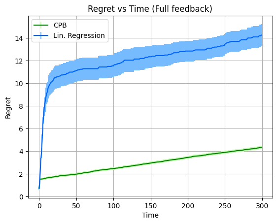
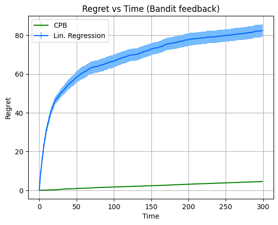
Refer to caption — Figure 1: The regret as a function of time in a) Full feedback setting, and b) Bandit feedback setting.

In our first experiment, full feedback is available, i.e. the samples $(\bm{x}_{t,i}^{T},v_{i,t})$ are available to both algorithms for all $i\in\mathcal{B},t\in[T]$ . In the second experiment the algorithms have bandit feedback. That is, a sample $(\bm{x}_{t,i}^{T},v_{i,t})$ is available for an algorithm only if box $i$ was opened at time $t$ by the algorithm. We plot the regret (defined in (2)) of the algorithms as a function of time $t$ . As expected, the regret of both algorithms is smaller under full feedback, since there is more information available at each round. In addition, the regret increases with sublinear rate as $t$ grows, which is compatible with our theoretical guarantees in both the full-feedback and the bandit setting. Finally, in both settings, using the $\mathcal{CPB}$ algorithm leads to significantly smaller regret compared to linear regression.

A.2 Impossibility beyond Realizability

We now provide an example to indicate that without the realizability assumption, our setting is not only computationally hard (even in the offline case) [Kearns et al., 1992], but also becomes information-theoretically hard in the online case:

Consider the simple setting of two boxes, with costs either $0$ or $1$ . The context provides us with some information on where is the $0$ in each round, and our objective it to select $0$ the maximum amount of times. Clearly, in the offline case the above setting coincides with that of agnostic learning, which is known to be computationally hard, even for linear functions (e.g., linear classification).

In the online setting, where an adversary can choose the context to give us at each round, the problem is information-theoretically hard. Similarly, assume that a context is a real number in $[0,1]$ and that there exists a threshold $x$ , which decides which box gives $0$ and which $1$ . The adversary can always give us a threshold in the uncertainty region, and force us to make a mistake at every round, thus accumulating linear cost over time, while the cost accumulated by the optimal algorithm (which knows the context-value relation) is 0.

A.3 Proofs from Section 3.1

See 3.2

Proof.

Assume we are using Weitzman’s Algorithm with reservation values $\bm{\sigma}$ in an instance with optimal reservation values $\bm{\sigma}^{*}$ and costs $\bm{c}$ . Let $\mathcal{P}$ be the set of boxes opened during the algorithm’s run. Then, the Pandora’s Box cost incurred at the end of the run can be bounded as follows:

	$\displaystyle\text{WEITZ}_{\bm{\mathcal{D}}}(\bm{\sigma};\bm{c})$	$\displaystyle=\mathbb{E}_{\bm{v}\sim\bm{\mathcal{D}}}\left[\min_{i\in{\mathcal{P}}}v_{i}+\sum_{i\in\mathcal{P}}c_{i}\right]$
		$\displaystyle=\mathbb{E}_{\bm{v}\sim\bm{\mathcal{D}}}\left[\min_{i\in{\mathcal{P}}}v_{i}+\sum_{i\in\mathcal{P}}c_{i}+c_{\mathcal{D}_{i}}(\sigma_{i})-c_{\mathcal{D}_{i}}(\sigma_{i})\right]$
		$\displaystyle=\text{WEITZ}_{\bm{\mathcal{D}}}(\bm{\sigma};\bm{c}_{\bm{\mathcal{D}}}(\bm{\sigma}))+\mathbb{E}_{\bm{v}\sim\bm{\mathcal{D}}}\left[\sum_{i\in{\mathcal{P}}}(c_{i}-c_{\mathcal{D}_{i}}(\sigma_{i}))\right]$
		$\displaystyle\leq\text{WEITZ}_{\bm{\mathcal{D}}}({\bm{\sigma}}^{*};\bm{c})+$
		$\displaystyle\qquad\mathbb{E}_{\bm{v}\sim\bm{\mathcal{D}}}\left[\sum_{i\in B}\textrm{ReLU}(c_{\mathcal{D}_{i}}(\sigma_{i})-c_{i})+\sum_{i\in{\mathcal{P}}}(c_{i}-c_{\mathcal{D}_{i}}(\sigma_{i}))\right]$
		$\displaystyle\leq\text{WEITZ}_{\bm{\mathcal{D}}}({\bm{\sigma}}^{*};\bm{c})+\mathbb{E}_{\bm{v}\sim\bm{\mathcal{D}}}\left[\sum_{i\in\mathcal{B}}\left\|c_{i}-c_{\mathcal{D}_{i}}(\sigma_{i})\right\|\right],$

where in the first inequality we used Lemma 3.3 and in the last inequality that every box from each of the sets $\mathcal{B}$ and $\mathcal{P}$ can contribute at most once in the sum, because of the ReLU function.∎

See 3.3

Proof.

Consider the optimal strategy $\text{WEITZ}_{\bm{\mathcal{D}}}(\bm{\sigma}^{*};\bm{c})$ for the instance with reservation values $\bm{\sigma}^{*}$ , and assume we use the same strategy in the instance where the ‘actual reservation values are $\hat{\bm{\sigma}}$ . That means our algorithm $\text{WEITZ}_{\bm{\mathcal{D}}}(\bm{\sigma}^{*};\bm{c}_{\bm{\mathcal{D}}}(\hat{\bm{\sigma}}))$ orders the boxes according to the reservation values $\bm{\sigma}^{*}$ and stops when $\min_{i}v_{i}\leq\sigma^{*}_{i+1}$ . Denote by $\mathcal{P}$ the set of boxes probed (opened) by the algorithm $\text{WEITZ}_{\bm{\mathcal{D}}}(\bm{\sigma}^{*};\bm{c}_{\bm{\mathcal{D}}}(\hat{\bm{\sigma}}))$ , then the cost is

	$\displaystyle\text{WEITZ}_{\bm{\mathcal{D}}}(\hat{\bm{\sigma}};\bm{c}_{\bm{\mathcal{D}}}(\hat{\bm{\sigma}}))$	$\displaystyle\leq\text{WEITZ}_{\bm{\mathcal{D}}}(\bm{\sigma}^{*};\bm{c}_{\bm{\mathcal{D}}}(\hat{\bm{\sigma}}))$
		$\displaystyle=\mathbb{E}_{\bm{v}\sim\bm{D}}\left[\min_{i\in\mathcal{P}}v_{i}+\sum_{i\in\mathcal{P}}c_{\mathcal{D}_{i}}(\hat{\sigma}_{i})\right]$
		$\displaystyle=\mathbb{E}_{\bm{v}\sim\bm{D}}\left[\min_{i\in\mathcal{P}}v_{i}\right]+\mathbb{E}_{\bm{v}\sim\bm{D}}\left[\sum_{i\in\mathcal{P}}c_{\mathcal{D}_{i}}(\hat{\sigma}_{i})-c_{\mathcal{D}_{i}}(\sigma^{}_{i})+c_{\mathcal{D}_{i}}(\sigma^{}_{i})\right]$
		$\displaystyle=\text{WEITZ}_{\bm{\mathcal{D}}}(\bm{\sigma}^{};\bm{c})+\sum_{i\in\mathcal{P}}(c_{\mathcal{D}_{i}}(\hat{\sigma}_{i})-c_{\mathcal{D}_{i}}(\sigma^{}_{i}))$
		$\displaystyle\leq\text{WEITZ}_{\bm{\mathcal{D}}}(\bm{\sigma}^{};\bm{c})+\sum_{i\in\mathcal{P}}\textrm{ReLU}(c_{\mathcal{D}_{i}}(\hat{\sigma}_{i})-c_{\mathcal{D}_{i}}(\sigma^{}_{i})),$

where the first inequality follows by the definition of the optimal, and the first equality is the actual cost of our algorithm, since in our instance we pay $c_{\mathcal{D}_{i}}(\hat{\sigma}_{i})$ for each box. ∎

A.4 Proofs from Section 3.2

See 3.4

Proof.

Recall from Definition 3 that

\displaystyle H_{c}(\sigma-v)=\frac{1}{2}\textrm{ReLU}(\sigma-v)^{2}-c(\sigma-v)=\left\{\begin{array}[]{lr}\frac{1}{2}(\sigma-v)^{2}-c(\sigma-v)&\text{if }\sigma\geq v\\ -c(\sigma-v),&\text{if }\sigma<v\end{array}\right\}

and

H^{\prime}_{c}(\sigma-v)=\textrm{ReLU}(\sigma-v)-c.

We also use that for $\sigma=\sigma^{*}$ using Weitzman’s theorem for optimal reservation values (Theorem 2.1) we have

\mathbb{E}_{v}\left[H^{\prime}_{c}(\sigma^{*}-v)\right]=0.

We need to compare $H_{c}(\sigma-v)-H_{c}(\sigma^{*}-v)$ to $|c_{D}(\sigma)-c_{D}(\sigma^{*})|$ . Using that $\int_{a}^{b}f^{\prime}(x)\,dx=f(b)-f(a)$ and changing the order between expectation and integration, we obtain

$\displaystyle\mathbb{E}_{v\sim D}\left[H_{c}(\sigma-v)-H_{c}(\sigma^{*}-v)\right]$	$\displaystyle=\mathbb{E}_{v\sim D}\left[\int_{\sigma^{*}}^{\sigma}H^{\prime}_{c}(\sigma^{\prime}-v)\,d\sigma^{\prime}\right]$
	$\displaystyle=\int_{\sigma^{*}}^{\sigma}\mathbb{E}_{v\sim D}\left[H^{\prime}_{c}(\sigma^{\prime}-v)\right]\,d\sigma^{\prime}$
	$\displaystyle=\int_{\sigma^{}}^{\sigma}\mathbb{E}_{v\sim D}\left[H^{\prime}_{c}(\sigma^{\prime}-v)\right]-\mathbb{E}_{v\sim D}\left[H^{\prime}_{c}(\sigma^{}-v)\right]\,d\sigma^{\prime}$
	$\displaystyle=\int_{\sigma^{}}^{\sigma}\mathbb{E}_{v\sim D}\left[\textrm{ReLU}(\sigma^{\prime}-v)\right]-\mathbb{E}_{v\sim D}\left[\textrm{ReLU}(\sigma^{}-v)\right]\,d\sigma^{\prime}$
	$\displaystyle=\int_{\sigma^{}}^{\sigma}(c_{D}(\sigma^{\prime})-c_{D}(\sigma^{}))\,d\sigma^{\prime},$	(4)

where the last inequality above is by definition of $c_{D}(\cdot)$ . We now distinguish between the following cases for the reservation value $\sigma$ compared to the optimal reservation value $\sigma^{*}$ .

Case $\sigma\geq\sigma^{*}$ :

observe that $c_{D}$ is 1-Lipschitz, therefore we have that $|c_{D}(\sigma)-c_{D}(\sigma^{\prime})|<|\sigma-\sigma^{\prime}|$ . Moreover, when $\sigma^{\prime}\geq\sigma^{*}$ we have $c_{D}(\sigma^{\prime})\geq c_{D}(\sigma^{*})$ . Thus Section A.4 becomes:

	$\displaystyle\mathbb{E}_{v\sim D}\left[H_{c}(\sigma-v)-H_{c}(\sigma^{*}-v)\right]$	$\displaystyle=\int_{\sigma^{}}^{\sigma}(c_{D}(\sigma^{\prime})-c_{D}(\sigma^{}))\,d\sigma^{\prime}$
		$\displaystyle\geq\int_{\sigma-(c_{D}(\sigma)-c_{D}(\sigma^{}))}^{\sigma}(c_{D}(\sigma^{\prime})-c_{D}(\sigma^{}))\,d\sigma^{\prime}$
		$\displaystyle\geq\int_{\sigma-(c_{D}(\sigma)-c_{D}(\sigma^{}))}^{\sigma}(c_{D}(\sigma)-c_{D}(\sigma^{})-(\sigma-\sigma^{\prime}))\,d\sigma^{\prime}$
		$\displaystyle=\frac{1}{2}(c_{D}(\sigma)-c_{D}(\sigma^{*}))^{2},$

where for the first inequality we used that $\sigma-\sigma^{*}\geq c_{D}(\sigma)-c_{D}(\sigma^{*})$ and for the second that $\sigma-\sigma^{\prime}\geq c_{D}(\sigma)-c_{D}(\sigma^{\prime})$ .

Case $\sigma<\sigma^{*}$ :

as before, Section A.4 can be written as

	$\displaystyle\mathbb{E}_{y\sim D}\left[H_{c}(\sigma-v)-H_{c}(\sigma^{*}-v)\right]$	$\displaystyle=\int_{\sigma^{}}^{\sigma}(c_{D}(\sigma^{\prime})-c_{D}(\sigma^{}))\,d\sigma^{\prime}$
		$\displaystyle=-\int_{\sigma}^{\sigma^{}}(c_{D}(\sigma^{\prime})-c_{D}(\sigma^{}))\,d\sigma^{\prime}$
		$\displaystyle\geq-\int_{\sigma}^{\sigma-(c_{D}(\sigma)-c_{D}(\sigma^{}))}(c_{D}(\sigma^{\prime})-c_{D}(\sigma^{}))\,d\sigma^{\prime}$
		$\displaystyle\geq\int_{\sigma}^{\sigma-(c_{D}(\sigma)-c_{D}(\sigma^{}))}(-c_{D}(\sigma)+c_{D}(\sigma^{})-(\sigma^{\prime}-\sigma))\,d\sigma^{\prime}$
		$\displaystyle=\frac{1}{2}(c_{D}(\sigma)-c_{D}(\sigma^{*}))^{2},$

where for the first inequality we used that $\sigma^{*}-\sigma\geq c_{D}(\sigma^{*})-c_{D}(\sigma)$ and the fact that $c_{D}(\sigma^{\prime})-c_{D}(\sigma^{*})\leq 0$ . For the second we used that $-c_{D}(\sigma^{\prime})\geq-c_{D}(\sigma)-(\sigma^{\prime}-\sigma)$ .

∎

A.5 Regression via FTRL and Proofs of Section 4.1

Recall our regression function defined in equation (2). We define $f_{t}:\mathbb{R}^{d}\rightarrow\mathbb{R}$ , as the loss function at time $t\in[T]$ as

f_{t}(\bm{w})=H_{c}(\bm{w}^{T}\bm{x}_{t}-y_{t})=\frac{1}{2}(\bm{w}^{T}\bm{x}_{t}-y_{t})_{+}^{2}-c(\bm{w}^{T}\bm{x}_{t}-y_{t}).

As these functions are convex, we can treat the problem as an online convex optimization. Specifically, the problem we solve is the following.

1.

At every round $t$ , we pick a vector $\bm{w}_{t}\in\mathbb{R}^{d}$ .
2.

An adversary picks a convex function $f_{t}:\mathbb{R}^{d}\rightarrow\mathbb{R}$ induced by the input-output pair $(\bm{x}_{t},y_{t})$ and we incur loss $f_{t}(\sigma_{t})$ .
3.

At the end of the round, we observe the function $f_{t}$ .

In order to solve this problem, we use a family of algorithms called Follow The Regularized Leader (FTRL). In these algorithms, at every step $t$ we pick the solution $\bm{w}_{t}$ that would have performed best so far while adding a regularization term $U(\bm{w}_{t})$ for stability reasons. That is, we choose

\bm{w}_{t}=\arg\min_{\bm{w}:\|w\|_{2}\leq M}\sum_{\tau=1}^{t-1}f_{t}(\bm{w})+U(\bm{w}).

The guarantees for these algorithms are presented in the following lemma.

Lemma A.1 (Theorem 2.11 from Shalev-Shwartz [2012]).

Let $f_{1},\ldots,f_{T}$ be a sequence of convex functions such that each $f_{t}$ is $L$ -Lipschitz with respect to some norm. Assume that FTRL is run on the sequence with a regularization function $U$ which is $\eta$ -strongly-convex with respect to the same norm. Then, for all $u\in C$ we have that $\text{Regret}(\text{FTRL},T)\cdot T\leq U_{\max}-U_{\min}+TL^{2}\eta$

Observe that in order to achieve the guarantees of Lemma A.1, we need the functions to have some convexity and Lipschitzness properties, for which we show the following lemma.

Lemma A.2.

The function $f_{t}(\bm{w})=H_{c}(\bm{w}^{T}\bm{x}_{t}-y_{t})$ is convex and $\max\{M,c\}$ -Lipschitz when $\|x_{t}\|_{2}\leq 1$ and $\|\bm{w}\|_{2}\leq M$ .

Proof of Lemma A.2.

We first show convexity and Lipschitzness for the function $H_{c}(z)=\frac{1}{2}\textrm{ReLU}(z)^{2}-cz$ for $z\in\mathbb{R}$ .

Consider the derivative $H^{\prime}_{c}(z)=\textrm{ReLU}(z)-c$ and the second derivative $H^{\prime\prime}_{c}(z)=\textbf{1}(z\geq 0)$ and notice that the second derivative is always non-negative which implies convexity.

To bound the Lipschitzness of $H_{c}$ , we consider the maximum absolute value of the derivative which is at most $\max\{c,\textrm{ReLU}(z)\}$ .

We now turn our attention to $f_{t}$ and notice that $f_{t}$ is convex as a composition of a convex function with a linear function. To show Lipschitzness we must bound the norm of the gradient of $f_{t}$ which is:

\|\nabla f_{t}(\bm{w})\|_{2}=|H^{\prime}_{c}(\bm{w}^{T}\bm{x}_{t}-y_{t})|\|\bm{x}\|_{2}\leq\max\{c,M\},

where the last inequality follows as the maximum value of $\bm{w}^{T}\bm{x}_{t}-y_{t}$ is at most $M$ . ∎

See 4.1

Proof.

We use the following regularizer $U(\bm{w})=\frac{1}{2\eta}||\bm{w}||_{2}^{2}$ , and observe that this is $\eta$ -strongly convex with $U_{\min}=0$ and $U_{\max}=M/(2\eta)$ . From Lemma A.2 we have that the loss function is convex and $\max\{c,M\}$ -Lipschitz, therefore using Lemma A.1 with $\eta=\frac{\sqrt{M}}{\max\{c,M\}\sqrt{2T}}$ we get that $\text{Regret}(FTRL,T)\leq\frac{M}{2\eta}+\eta(\max\{c,M\})^{2}T=\max\{c,M\}\sqrt{2MT}$ . ∎

See 4.2

Proof.

The regret of Contextual Pandora’s Box can be upper bounded as follows:

	$\displaystyle\text{Regret}(\mathcal{CPB},T)$	$\displaystyle\leq 2n\sqrt{Tr(T)}$	by Theorem 3.1
		$\displaystyle\leq 3n\sqrt{\max\{M,c\}}M^{1/4}T^{\frac{3}{4}}.$	by Lemma 4.1

∎

A.6 Proofs from Section 4.2

In this section we show how to obtain the guarantees of FTRL in the case of costly feedback proving Lemma 4.3.

While the proof is standalone, the analysis uses ideas from Gergatsouli and Tzamos [2022] (in particular Lemma 4.2 and Algorithm 2). We give a simplified presentation for the case of online regression with improved bounds.

See 4.3

Proof.

Recall that in the online regression problem, we obtain loss $f_{t}$ at any time step where $f_{t}(\bm{w})=H_{c}(\bm{w}^{T}\bm{x}_{t}-y_{t})=\frac{1}{2}\textrm{ReLU}(\bm{w}^{T}\bm{x}_{t}-y_{t})^{2}-c(\bm{w}^{T}\bm{x}_{t}-y_{t})$ .

To analyze the regret for the costly feedback setting, we consider the regret of two related settings for a full-information online learner but with smaller number of time steps $T/k$ .

1.

Average costs setting: the learner observes at each round $\tau$ a single function

$\overline{f}_{\tau}=\frac{1}{k}\sum_{t\in\mathcal{I}_{\tau}}f_{t},$

which is the average of the $k$ functions in the corresponding interval $\mathcal{I}_{\tau}$ .
2.

Random costs setting: the learner observes at each round $\tau$ a single function

$f^{r}_{\tau}=f_{t_{p}}\quad\text{with}\quad t_{p}\sim\text{Uniform}(\mathcal{I}_{\tau})$

sampled uniformly among the $k$ functions $f_{t}$ for $t\in\mathcal{I}_{\tau}$ .

The guarantee of the full information oracle implies that for the random costs setting we obtain regret $r(T/k)$ . That is, the oracle chooses a sequence $\bm{w}_{1},\ldots,\bm{w}_{T/k}$ such that

\sum_{\tau=1}^{T/k}f^{r}_{\tau}(\bm{w}_{\tau})\leq\min_{\bm{w}}\sum_{\tau=1}^{T/k}f^{r}_{\tau}(\bm{w})+r(T/k).

Denote by $\bm{w}^{*}=\text{argmin}_{\bm{w}\in\mathbb{R}^{d}}\sum_{\tau=1}^{T/k}\overline{f}_{\tau}(\bm{w})$ be the minimizer of the $\overline{f}_{t}$ over the $T/k$ rounds. Note that this is also the minimizer of $\sum_{t=1}^{T}{f}_{t}(\bm{w})$ . From the above regret guarantee, we get that

\sum_{\tau=1}^{T/k}(f^{r}_{\tau}(\bm{w}_{\tau})-f^{r}_{\tau}(\bm{w}^{*}))\leq r(T/k).

Since $\mathbb{E}\left[f^{r}_{\tau}(\bm{z}_{\tau})\right]=\overline{f}_{\tau}(\bm{z}_{\tau})$ when the expectation is over the choice of $t_{p}\sim\text{Uniform}(\mathcal{I}_{\tau})$ . Taking expectation in the above, we get that

\sum_{\tau=1}^{T/k}(\overline{f}_{\tau}(\bm{w}_{\tau})-\overline{f}_{\tau}(\bm{w}^{*}))\leq r(T/k),

which implies that the regret in the average costs setting is also $r(T/k)$ .

We now obtain the final result by noticing that the regret of the algorithm is at most $k$ times the regret of the average costs setting and incurs an additional overhead of $\frac{T}{k}c$ for the information acquisition cost in the $T/k$ rounds where the input-output pairs are queried. Thus, overall the regret is bounded by $kr(T/k)+cT/k$ . ∎

See 4.4

Proof.

Initially observe that by combining Lemma 4.1 and Lemma 4.3 we get that there exists an oracle for online regression with loss $H_{c}$ under the costly feedback setting that guarantees

\displaystyle\text{Regret}(\mathcal{O}_{\text{costly}},T)

\displaystyle\leq L\sqrt{2kMT}+cT/k

with $L=\max\{M,c\}$ . Setting $k=\left(\frac{Tc^{2}}{2ML^{2}}\right)^{1/3}$ , we obtain regret $(2cML^{2})^{1/3}T^{2/3}$ . Further combining this with Theorem 3.1 that connects the regret guarantees of regression with the regret for our Contextual Pandora’s Box algorithm, we obtain regret $2n(2c_{\max}M\max\{M,c_{\max}\}^{2})^{1/6}T^{5/6}$ . ∎

A.7 Discussion on the Lower Bounds

In this work our goal was to formulate the online contextual extension of the Pandora’s Box problem and design no-regret algorithms for this problem, and therefore we left the lower bounds as a future work direction. We are however including here a brief discussion on lower bounds implied by previous work.

In Gatmiry et al. [2024] the authors study a special case of our setting where the value distributions and contexts are fixed at every round and for each alternative. The results of Gatmiry et al. [2024] imply a lower bound for this very special case of our problem, which however does not correspond to an adversarial setting, as our general formulation does. Notice, also, that a $\sqrt{T}$ lower bound for our problem can be directly obtained by the fact that our setting generalizes the stochastic multi-armed bandit problem. Observe that if all costs are chosen to be identical and large enough, then both the player and the optimal solution must select exactly one alternative per round (and their inspection costs cancel out in the regret). Interestingly, in that case Weitzman’s algorithm indeed selects the alternative of the smallest mean reward.

In another related setting, multi-armed bandits with paid observations, Seldin et al. [2014] show a $T^{2/3}$ lower bound on the regret in the adversarial case. Although their setting is different (e.g. in our setting multiple actions are allowed at each round and there is contextual information involved) we believe that it has similarities to ours in terms of costly options and information acquisition. Therefore, we believe that tighter lower bounds could hold for our general adversarial problem.

A.8 A primer on Pandora’s Box

We include here a more detailed discussion on Pandora’s Box problem for anyone unfamiliar with the setting.

This problem was first formulated by Weitzman Weitzman [1979] in the following form; there are $n$ boxes, each box $i$ has a deterministic opening cost $c_{i}\geq 0$ and a value that follows a known distribution $\mathcal{D}_{i}$ . The player can observe the value instantiated by the distribution of a box after paying the opening cost. The goal is to select boxes to open, and a value to keep so as to maximize

\mathbb{E}_{\mathcal{P},\mathcal{D}}\left[\max_{i\in\mathcal{P}}v_{i}+\sum_{i\in\mathcal{P}}c_{i}\right]

In the original problem, the distributions $\mathcal{D}_{i}$ are independent, and the optimal algorithm is given by Algorithm 4. In the algorithm Weitzman used the reservation value for each box $i$ which is a number calculated as the solution to the equation $\mathbb{E}_{\mathcal{D_{i}}}\left[(v-\sigma_{i})^{+}\right]=c_{i}$ , and as shown in Weitzman [1979], this is enough to produce an optimal solution through Algorithm 4. In our work we tackle the minimization version of the problem (similarly to Chawla et al. [2020], Gergatsouli and Tzamos [2022], Chawla et al. [2023]), described in more detail in Section 2. For the independent case the same results hold regardless of the version and in Algorithm 4 we highlighted the differences with Algorithm 1 to show the changes required for the maximization.

1 Input:

n

boxes, costs

c_{i}

, reservation values

\sigma_{i}

for

i\in\mathcal{B}

21:

\pi\leftarrow

sort boxes by decreasing

\sigma_{i}

32:

v_{\textbf{max}}\leftarrow 0

3: for every box

\pi_{i}

44: Pay

c_{i}

and open box

\pi_{i}

and observe

v_{i}

55:

v_{\textbf{max}}\leftarrow\textbf{max}(v_{\textbf{max}},v_{i})

6: if

v_{\textbf{max}}<{\sigma}_{\pi_{i+1}}

then

7: Stop and collect

v_{\textbf{max}}

8: end if

9: end for

Algorithm 4 Weitzman’s algorithm.

For a summary of the recent work on Pandora’s Box see the survey Beyhaghi and Cai [2023].

	$\displaystyle\mathbb{E}_{v\sim D}\left[H_{c}(\sigma-v)-H_{c}(\sigma^{*}-v)\right]$	$\displaystyle=\int_{\sigma^{}}^{\sigma}(c_{D}(\sigma^{\prime})-c_{D}(\sigma^{}))\,d\sigma^{\prime}$
		$\displaystyle\geq\int_{\sigma-(c_{D}(\sigma)-c_{D}(\sigma^{}))}^{\sigma}(c_{D}(\sigma^{\prime})-c_{D}(\sigma^{}))\,d\sigma^{\prime}$
		$\displaystyle\geq\int_{\sigma-(c_{D}(\sigma)-c_{D}(\sigma^{}))}^{\sigma}(c_{D}(\sigma)-c_{D}(\sigma^{})-(\sigma-\sigma^{\prime}))\,d\sigma^{\prime}$
		$\displaystyle=\frac{1}{2}(c_{D}(\sigma)-c_{D}(\sigma^{*}))^{2},$

	$\displaystyle\mathbb{E}_{y\sim D}\left[H_{c}(\sigma-v)-H_{c}(\sigma^{*}-v)\right]$	$\displaystyle=\int_{\sigma^{}}^{\sigma}(c_{D}(\sigma^{\prime})-c_{D}(\sigma^{}))\,d\sigma^{\prime}$
		$\displaystyle=-\int_{\sigma}^{\sigma^{}}(c_{D}(\sigma^{\prime})-c_{D}(\sigma^{}))\,d\sigma^{\prime}$
		$\displaystyle\geq-\int_{\sigma}^{\sigma-(c_{D}(\sigma)-c_{D}(\sigma^{}))}(c_{D}(\sigma^{\prime})-c_{D}(\sigma^{}))\,d\sigma^{\prime}$
		$\displaystyle\geq\int_{\sigma}^{\sigma-(c_{D}(\sigma)-c_{D}(\sigma^{}))}(-c_{D}(\sigma)+c_{D}(\sigma^{})-(\sigma^{\prime}-\sigma))\,d\sigma^{\prime}$
		$\displaystyle=\frac{1}{2}(c_{D}(\sigma)-c_{D}(\sigma^{*}))^{2},$

Contextual Pandora’s Box

Abstract

1 Introduction

Realizability.

1.1 Our Contribution

Main Theorem (Informal).

1.2 Related Work

2 Problem Definition and Notation

2.1 Original Pandora’s Box Formulation

Definition 1 (Pandora’s Box cost).

Theorem 2.1 (Weitzman (1979)).

2.2 Online Contextual Pandora’s Box

Assumption 2.2 (Realizability).

Definition 2 (Expected Regret).

Remark.

3 Reduction to Online Regression

Definition 3 (Linear-Quadratic Online Regression).

Theorem 3.1.

3.1 Weitzman’s Robustness

Definition 4 (Approximate Cost).

Remark.

Proposition 3.2.

Lemma 3.3.

3.2 Proof of Theorem 3.1

Lemma 3.4.

Proof of Theorem 3.1.

4 Linear Contextual Pandora’s Box

4.1 Full Information Setting

Lemma 4.1.

Theorem 4.2.

4.2 Bandit Setting

Lemma 4.3.

Theorem 4.4.

5 Conclusion and Further Directions

References

Appendix A Appendix

A.1 Experiments

A.2 Impossibility beyond Realizability

A.3 Proofs from Section 3.1

Proof.

Proof.

A.4 Proofs from Section 3.2

Proof.

Case σ≥σ∗\sigma\geq\sigma^{*}:

Case σ<σ∗\sigma<\sigma^{*}:

A.5 Regression via FTRL and Proofs of Section 4.1

Lemma A.1 (Theorem 2.11 from Shalev-Shwartz [2012]).

Lemma A.2.

Proof of Lemma A.2.

Proof.

Proof.

A.6 Proofs from Section 4.2

Proof.

Proof.

A.7 Discussion on the Lower Bounds

A.8 A primer on Pandora’s Box

Case $\sigma\geq\sigma^{*}$ :

Case $\sigma<\sigma^{*}$ :