Contextual quantum metrology
Abstract
Quantum metrology promises higher precision measurements than classical methods. Entanglement has been identified as one of quantum resources to enhance metrological precision. However, generating entangled states with high fidelity presents considerable challenges, and thus attaining metrological enhancement through entanglement is generally difficult. Here, we show that contextuality of measurement selection can enhance metrological precision, and this enhancement is attainable with a simple linear optical experiment. We call our methodology “contextual quantum metrology” (coQM). Contextuality is a nonclassical property known as a resource for various quantum information processing tasks. Until now, it has remained an open question whether contextuality can be a resource for quantum metrology. We answer this question in the affirmative by showing that the coQM can elevate precision of an optical polarimetry by a factor of to , much higher than the one by quantum Fisher information, known as the limit of conventional quantum metrology. We achieve the contextuality-enabled enhancement with two polarization measurements which are mutually complementary, whereas, in the conventional method, some optimal measurements to achieve the precision limit are either theoretically difficult to find or experimentally infeasible. These results highlight that the contextuality of measurement selection is applicable in practice for quantum metrology.
Introduction
Precision measurement has played a crucial role in the development of natural science and engineering since measurement is a means for observing nature. As a technology for precision measurement, quantum metrology has recently drawn attention with a wide range of applications such as microscopy [1], imaging [2, 3], patterning [4, 5], gravitational wave detection [6, 7, 8], and time keeping [9, 10]. Quantum metrology enables measurements going beyond precision of the standard quantum limit which can be obtained from the most-classical state in quantum physics. One of the resources for the precision enhancement is entanglement, a nonclassical property of quantum states [11, 12, 13, 14]. However, an entangled state can easily lose its property through interaction with other objects, while the interaction is inevitable in metrology. This makes it challenging to generate and manipulate an entangled state. Due to the limitations, it is difficult in practice to attain the entanglement-enabled enhancement of precision. If easy-to-implement resources for metrology are found, the performance of quantum metrology can be greatly enhanced, as well as its practicality. In this work, we demonstrate that contextuality of measurement selection [15], another nonclassical property, is an easy-to-implement resource for quantum metrology.
Specifically, contextuality here refers to dependency of quantum systems on measurement context [16]. Unlike classical predictions, quantum predictions for a given measurement can change depending on whether another measurement is performed simultaneously or not. Bell-Kochen-Specker theorem first showed that quantum physics is contextual [17, 18], and this has been experimentally proved on various quantum systems [19, 20, 21, 22]. Also, it has been revealed that the contextuality can be a resource for quantum information processing tasks such as quantum key distribution [23, 24], universal quantum computing [25], quantum state discrimination [26], and quantum machine learning [27, 28]. Yet, whether the contextuality can be a resource for quantum metrology remains a question.
To demonstrate the precision enhancement from the contextuality of measurement selection, we propose a method which we call contextual quantum metrology (coQM). Unlike conventional quantum metrology, the coQM utilizes two measurement settings and their contextuality. In our experiment, we adopt an optical polarimetry devised to measure concentration of sucrose solution [29], and modify its scheme for the coQM. Our experiment employs two polarization measurements in mutually unbiased (or complementary) bases, and their selection context is implemented by toggling a polarizing beam splitter ‘in’ and ‘out’ from its optical path. Our setup is scalable in that the size of the experiment does not increase along with the increase of the number of probe photons. Also, the enhanced precision is attainable without error correction or mitigation which requires overhead [30, 31]. We finally show that the precision of coQM can go beyond the precision limit of conventional quantum metrology [32, 33, 34] by a factor of to .
Contextual quantum metrology
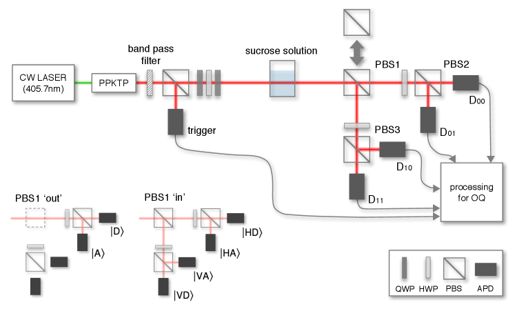
Fig. 1 shows an experimental schematic for the coQM. Here, the coQM estimates the concentration of sucrose solution by following four steps: preparing a polarized single photon as a probe light (see Methods), interacting the photon with the sucrose solution, measuring the polarization, and calculating an estimate via maximum likelihood estimator (MLE) using the operational quasiprobability which will be discussed later as in Eq. (1). The photon interacts with the sucrose solution as it propagates through the solution. Afterwards, the photon polarization rotates by angle , where , , and are the specific rotation of the sucrose solution, the concentration of the solution, and traveling length of light in the solution, respectively [29]. We can decide the concentration by measuring the polarization change for a given specific rotation and traveling length. All the procedures here look similar to those of the conventional quantum metrology [35], but the measurement and the estimation are steps that differentiate the coQM from the conventional approach.
In the measurement step, the coQM employs two different polarization measurement settings and to utilize the contextuality of measurement selection therefrom [15]. measures the polarization in a specific basis and does in a basis tilted from the basis of by half-wave plate. Our basic setup is the measurement by , and we consider a context of whether measurement is selected to be performed or not, prior to performing . If is not selected, the measurement only is performed, and probability is given by for a binary value . If is selected, the experimental setup runs the consecutive measurement performing first and later. In this case, probability is given by for an outcome pair , where is a binary outcome of . In our experiment (Fig. 1), the context of selecting is implemented by toggling ‘in’ and ’out’ the state of polarizing beam splitter PBS. Depending on the context, the quantum prediction of measurement changes, so the two probabilities by only and by the consecutive differ in general, i.e., [36]. (We will discuss that this difference stems from the incompatibility of measurements [37].) Our metrology utilizes this effect to enhance precision of the polarimetry.
In the estimation step, we employ a noncontextual (or context-free) model, so-called operational quasiprobability [38, 39], which is given by
| (1) |
The context-free condition in our measurement setup is to assume that the prediction of measurement is invariant under the context of selecting the measurement . This is called the condition of no-signaling in time represented by , [36]. The crucial property of the operational quasiprobability is that, for the context-free condition, is reduced to the probability by the consecutive measurement, , . To the contrary, the quantum predictions violate the condition in general, , and can even be negative-valued [38, 39].
The conventional quantum metrology estimates a physical parameter with an estimator based on a conditional probability for a data set (see Supplementary Information). In the coQM, the operational quasiprobability plays a role of the conditional probability for the two data sets and . In other words, the coQM calculates an estimate of polarization with a maximum likelihood estimator given by
| (2) |
where is a log-likelihood function for (see Methods). The possible problem caused by this replacement is that can be negative unlike the conditional probability, so that the log-likelihood function diverges. However, we find that remains positive for some range of parameters. We focus on the case for to be applicable to the log-likelihood function without the divergence problem. Finally, for an initial polarization , we derive the estimate of concentration from the polarization change as .
Results
Our goal is to demonstrate outperformance of the coQM over the conventional quantum metrology. We employ error of estimate , the standard deviation that the estimate differs from the actual value, to quantify the performance of estimation. The smaller the error is, the more precise the estimate is.
As a baseline of performance, we take the conventional quantum metrology and its error given by quantum Fisher information (QFI) , , where is the number of samples. This is known as the lower bound of error in the conventional method. In the coQM, we propose contextual Fisher information (coFI) to quantify the performance of the coQM,
| (3) |
In the asymptotic limit of , the error of the coQM approaches to (see Supplementary Information for the asymptotic property and estimator of coFI).
Contextuality-enabled enhancement The coQM gains precision enhancement over the conventional quantum metrology if
| (4) |
Our method uses the two data sets and . If each data set collects samples, the total number of samples is in our method. Reduction factor in the error by the conventional is introduced, assuming the conventional takes samples (which is equivalent to comparing to ).
We here suggest specific cases satisfying the criterion (4). Instead of a theoretical proof, we briefly summarize the theory behind the enhancement of precision by following arguments: For the noncontextual model, the operational quasiprobability becomes the joint probability of the consecutive measurement . In this case, the coQM is reduced and equivalent to the conventional quantum metrology using the consecutive measurement so that the equals or larger than (see Supplementary Information). For the contextual model, conversely, can be smaller than (see Ref. [40] for rigorous discussions). Fig. 2 a shows simulation results of the contextuality-enabled enhancement on the Bloch sphere.
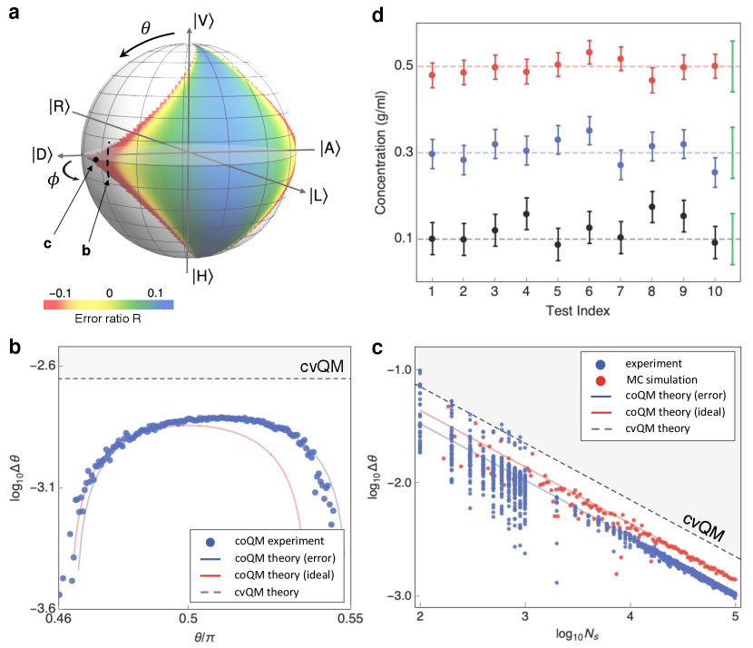
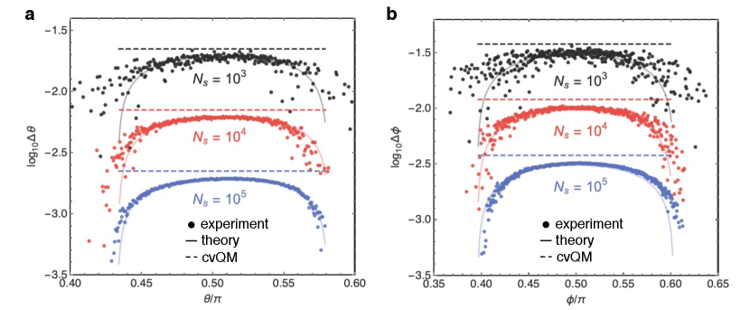
We perform polarization estimation of with probe states prepared in for and . For the probe states, the operational quasiprobability is given by . We draw samples for each data set to construct the operational quasiprobability, and calculate an estimate with the estimator (2). For polarization estimation of , QFI , so the coQM gains the contextuality-enabled enhancement if . The errors of the coQM are smaller than the error limit of the conventional quantum metrology for the whole selected range of (Fig. 2 ). The worst case in our results has around , and the best case has around each end of the range of . This demonstrates that our method elevates the precision of polarimetry by factor of to from the limit of conventional quantum metrology.
We estimate sucrose solutions of three different concentrations , and g ml-1. We prepare the probe state with initial parameters and . For each concentration, we repeat the estimation times. The results (Fig. 2 d) show that the errors of estimates by the coQM, , are smaller than the minimum error by the conventional quantum metrology (); For , and g ml-1, the mean errors are , , and , respectively. This illustrates that the coQM exceeds the conventional quantum metrology by a wide margin.
Measurement Incompatibility
The contextuality of measurement selection stems from the incompatibility of quantum measurements [37]. In the scenario of the consecutive measurement, if the two measurements and commute, the consecutive measurement is de facto a single measurement; the probabilities and are equal and the prediction for is noncontextual. Otherwise, the prediction for the measurement depends on whether performing the first measurement and it is contextual except for a case when the initial state is prepared in an eigenstate of the . Thus, the measurement incompatibility is necessary for the contextuality of measurement selection.
The noncommutation of observable operators defines the incompatibility among measurements, represented by projection-valued measures (PVM), which we assume in the present work. The notion of incompatibility needs to be generalized if the representation of measurement is generalized to positive operator-valued measure (POVM). This generalization is required, for example, if one considers an open quantum system in a noisy environment. Non-joint measurability (non-JM) is one of the generalizations [37]. The non-JM plays an important role in a contextuality [41, 42], as does the noncommutativity [43]. In fact, non-JM and the contextuality of measurement selection are also closely related as the negativity of operational quasiprobability is the necessary and sufficient condition for non-JM [44, 40].
Recently, there were studies in a similar vein to the present work [45, 46], showing that the noncommutativity can be a resource for quantum metrology. However, their schemes employ a post-selection to discard unwanted measurement outcomes, so there is a tradeoff between success probability and Fisher information; success probability becomes small if Fisher information is large [47]. Quantum post-selected metrology such as weak value amplification methods share this matter [48, 49]. On the contrary, our method utilizes all of measurement outcomes for the estimation [38, 39], implying that the coQM is free from such tradeoff.
Outlook
This work demonstrates that utilizing the contextuality of measurement selection can enhance the precision measurement. The experiment attains precision beyond the limit of conventional quantum metrology [33, 34]. The coQM has advantages over the conventional method (see Supplementary Information): it can enhance the precision without optimizing the measurements if they are incompatible, and it works even without any entangled state of probe that has been regarded difficult to generate and manipulate. We use the heralded single-photon source to clearly show the performance of coQM per a unit particle of probe. We expect that a multi-photon source can also be adopted for the coQM with the similar settings of measurements [15]. Our method is expected to be applicable to a quantum sensor [50] if the context of measurement selection can be implemented within the sensor’s system. In addition, the approaches employed to demonstrate the contextuality-enabled enhancements can be utilized to characterize quantum devices (see Supplementary Information), which is a fundamental task required to implement quantum technologies.
References
- Casacio et al. [2021] C. A. Casacio, L. S. Madsen, A. Terrasson, M. Waleed, K. Barnscheidt, B. Hage, M. A. Taylor, and W. P. Bowen, Quantum-enhanced nonlinear microscopy, Nature 594, 201 (2021).
- Treps et al. [2002] N. Treps, U. Andersen, B. Buchler, P. K. Lam, A. Maître, H.-A. Bachor, and C. Fabre, Surpassing the standard quantum limit for optical imaging using nonclassical multimode light, Phys. Rev. Lett. 88, 203601 (2002).
- Brida et al. [2010] G. Brida, M. Genovese, and I. Ruo Berchera, Experimental realization of sub-shot-noise quantum imaging, Nature Photonics 4, 227 (2010).
- Boto et al. [2000] A. N. Boto, P. Kok, D. S. Abrams, S. L. Braunstein, C. P. Williams, and J. P. Dowling, Quantum interferometric optical lithography: Exploiting entanglement to beat the diffraction limit, Phys. Rev. Lett. 85, 2733 (2000).
- Parniak et al. [2018] M. Parniak, S. Borówka, K. Boroszko, W. Wasilewski, K. Banaszek, and R. Demkowicz-Dobrzański, Beating the rayleigh limit using two-photon interference, Phys. Rev. Lett. 121, 250503 (2018).
- Abramovici et al. [1992] A. Abramovici, W. E. Althouse, R. W. P. Drever, Y. Gürsel, S. Kawamura, F. J. Raab, D. Shoemaker, L. Sievers, R. E. Spero, K. S. Thorne, R. E. Vogt, R. Weiss, S. E. Whitcomb, and M. E. Zucker, Ligo: The laser interferometer gravitational-wave observatory, Science 256, 325 (1992).
- Collaboration [2011] T. L. S. Collaboration, A gravitational wave observatory operating beyond the quantum shot-noise limit, Nature Physics 7, 962 (2011).
- Aasi et al. [2013] J. Aasi, J. Abadie, B. P. Abbott, R. Abbott, T. D. Abbott, M. R. Abernathy, C. Adams, T. Adams, P. Addesso, R. X. Adhikari, C. Affeldt, O. D. Aguiar, P. Ajith, B. Allen, E. Amador Ceron, D. Amariutei, S. B. Anderson, W. G. Anderson, K. Arai, M. C. Araya, C. Arceneaux, S. Ast, S. M. Aston, D. Atkinson, P. Aufmuth, C. Aulbert, L. Austin, B. E. Aylott, S. Babak, P. T. Baker, S. Ballmer, Y. Bao, J. C. Barayoga, D. Barker, B. Barr, L. Barsotti, M. A. Barton, I. Bartos, R. Bassiri, J. Batch, J. Bauchrowitz, B. Behnke, A. S. Bell, C. Bell, G. Bergmann, J. M. Berliner, A. Bertolini, J. Betzwieser, N. Beveridge, P. T. Beyersdorf, T. Bhadbhade, I. A. Bilenko, G. Billingsley, J. Birch, S. Biscans, E. Black, J. K. Blackburn, L. Blackburn, D. Blair, B. Bland, O. Bock, T. P. Bodiya, C. Bogan, C. Bond, R. Bork, M. Born, S. Bose, J. Bowers, P. R. Brady, V. B. Braginsky, J. E. Brau, J. Breyer, D. O. Bridges, M. Brinkmann, M. Britzger, A. F. Brooks, D. A. Brown, D. D. Brown, K. Buckland, F. Brückner, B. C. Buchler, A. Buonanno, J. Burguet-Castell, R. L. Byer, L. Cadonati, J. B. Camp, P. Campsie, K. Cannon, J. Cao, C. D. Capano, L. Carbone, S. Caride, A. D. Castiglia, S. Caudill, M. Cavaglià, C. Cepeda, T. Chalermsongsak, S. Chao, P. Charlton, X. Chen, Y. Chen, H.-S. Cho, J. H. Chow, N. Christensen, Q. Chu, S. S. Y. Chua, C. T. Y. Chung, G. Ciani, F. Clara, D. E. Clark, J. A. Clark, M. Constancio Junior, D. Cook, T. R. Corbitt, M. Cordier, N. Cornish, A. Corsi, C. A. Costa, M. W. Coughlin, S. Countryman, P. Couvares, D. M. Coward, M. Cowart, D. C. Coyne, K. Craig, J. D. E. Creighton, T. D. Creighton, A. Cumming, L. Cunningham, K. Dahl, M. Damjanic, S. L. Danilishin, K. Danzmann, B. Daudert, H. Daveloza, G. S. Davies, E. J. Daw, T. Dayanga, E. Deleeuw, T. Denker, T. Dent, V. Dergachev, R. DeRosa, R. DeSalvo, S. Dhurandhar, I. Di Palma, M. Díaz, A. Dietz, F. Donovan, K. L. Dooley, S. Doravari, S. Drasco, R. W. P. Drever, J. C. Driggers, Z. Du, J.-C. Dumas, S. Dwyer, T. Eberle, M. Edwards, A. Effler, P. Ehrens, S. S. Eikenberry, R. Engel, R. Essick, T. Etzel, K. Evans, M. Evans, T. Evans, M. Factourovich, S. Fairhurst, Q. Fang, B. F. Farr, W. Farr, M. Favata, D. Fazi, H. Fehrmann, D. Feldbaum, L. S. Finn, R. P. Fisher, S. Foley, E. Forsi, N. Fotopoulos, M. Frede, M. A. Frei, Z. Frei, A. Freise, R. Frey, T. T. Fricke, D. Friedrich, P. Fritschel, V. V. Frolov, M.-K. Fujimoto, P. J. Fulda, M. Fyffe, J. Gair, J. Garcia, N. Gehrels, G. Gelencser, L. Á. Gergely, S. Ghosh, J. A. Giaime, S. Giampanis, K. D. Giardina, S. Gil-Casanova, C. Gill, J. Gleason, E. Goetz, G. González, N. Gordon, M. L. Gorodetsky, S. Gossan, S. Goßler, C. Graef, P. B. Graff, A. Grant, S. Gras, C. Gray, R. J. S. Greenhalgh, A. M. Gretarsson, C. Griffo, H. Grote, K. Grover, S. Grunewald, C. Guido, E. K. Gustafson, R. Gustafson, D. Hammer, G. Hammond, J. Hanks, C. Hanna, J. Hanson, K. Haris, J. Harms, G. M. Harry, I. W. Harry, E. D. Harstad, M. T. Hartman, K. Haughian, K. Hayama, J. Heefner, M. C. Heintze, M. A. Hendry, I. S. Heng, A. W. Heptonstall, M. Heurs, M. Hewitson, S. Hild, D. Hoak, K. A. Hodge, K. Holt, M. Holtrop, T. Hong, S. Hooper, J. Hough, E. J. Howell, V. Huang, E. A. Huerta, B. Hughey, S. H. Huttner, M. Huynh, T. Huynh-Dinh, D. R. Ingram, R. Inta, T. Isogai, A. Ivanov, B. R. Iyer, K. Izumi, M. Jacobson, E. James, H. Jang, Y. J. Jang, E. Jesse, W. W. Johnson, D. Jones, D. I. Jones, R. Jones, L. Ju, P. Kalmus, V. Kalogera, S. Kandhasamy, G. Kang, J. B. Kanner, R. Kasturi, E. Katsavounidis, W. Katzman, H. Kaufer, K. Kawabe, S. Kawamura, F. Kawazoe, D. Keitel, D. B. Kelley, W. Kells, D. G. Keppel, A. Khalaidovski, F. Y. Khalili, E. A. Khazanov, B. K. Kim, C. Kim, K. Kim, and N. Kim, Enhanced sensitivity of the ligo gravitational wave detector by using squeezed states of light, Nature Photonics 7, 613 (2013).
- Giovannetti et al. [2001] V. Giovannetti, S. Lloyd, and L. Maccone, Quantum-enhanced positioning and clock synchronization, Nature 412, 417 (2001).
- Pedrozo-Peñafiel et al. [2020] E. Pedrozo-Peñafiel, S. Colombo, C. Shu, A. F. Adiyatullin, Z. Li, E. Mendez, B. Braverman, A. Kawasaki, D. Akamatsu, Y. Xiao, and V. Vuletić, Entanglement on an optical atomic-clock transition, Nature 588, 414 (2020).
- Giovannetti et al. [2004] V. Giovannetti, S. Lloyd, and L. Maccone, Quantum-enhanced measurements: Beating the standard quantum limit, Science 306, 1330 (2004), https://www.science.org/doi/pdf/10.1126/science.1104149 .
- Giovannetti et al. [2006] V. Giovannetti, S. Lloyd, and L. Maccone, Quantum metrology, Phys. Rev. Lett. 96, 010401 (2006).
- Giovannetti et al. [2011] V. Giovannetti, S. Lloyd, and L. Maccone, Advances in quantum metrology, Nature Photonics 5, 222 (2011).
- Tan and Jeong [2019] K. C. Tan and H. Jeong, Nonclassical light and metrological power: An introductory review, AVS Quantum Science 1, 014701 (2019).
- Ryu et al. [2019] J. Ryu, S. Hong, J.-S. Lee, K. H. Seol, J. Jae, J. Lim, J. Lee, K.-G. Lee, and J. Lee, Optical experiment to test negative probability in context of quantum-measurement selection, Scientific Reports 9, 10.1038/s41598-019-53121-5 (2019).
- Spekkens [2005] R. W. Spekkens, Contextuality for preparations, transformations, and unsharp measurements, Phys. Rev. A 71, 052108 (2005).
- Bell [1964] J. S. Bell, On the Einstein-Podolsky-Rosen paradox, Physics 1, 195 (1964).
- Kochen and Specker [1967] S. Kochen and E. P. Specker, The problem of hidden variables in quantum mechanics, Journal of Mathematics and Mechanics 17, 59 (1967).
- Hasegawa et al. [2006] Y. Hasegawa, R. Loidl, G. Badurek, M. Baron, and H. Rauch, Quantum contextuality in a single-neutron optical experiment, Phys. Rev. Lett. 97, 230401 (2006).
- Kirchmair et al. [2009] G. Kirchmair, F. Zähringer, R. Gerritsma, M. Kleinmann, O. Gühne, A. Cabello, R. Blatt, and C. F. Roos, State-independent experimental test of quantum contextuality, Nature 460, 494 (2009).
- Jerger et al. [2016] M. Jerger, Y. Reshitnyk, M. Oppliger, A. Potočnik, M. Mondal, A. Wallraff, K. Goodenough, S. Wehner, K. Juliusson, N. K. Langford, and A. Fedorov, Contextuality without nonlocality in a superconducting quantum system, Nature Communications 7, 12930 (2016).
- Zhang et al. [2019] A. Zhang, H. Xu, J. Xie, H. Zhang, B. J. Smith, M. S. Kim, and L. Zhang, Experimental test of contextuality in quantum and classical systems, Phys. Rev. Lett. 122, 080401 (2019).
- Acín et al. [2007] A. Acín, N. Brunner, N. Gisin, S. Massar, S. Pironio, and V. Scarani, Device-independent security of quantum cryptography against collective attacks, Phys. Rev. Lett. 98, 230501 (2007).
- Reichardt et al. [2013] B. W. Reichardt, F. Unger, and U. Vazirani, Classical command of quantum systems, Nature 496, 456 (2013).
- Howard et al. [2014] M. Howard, J. Wallman, V. Veitch, and J. Emerson, Contextuality supplies the ‘magic’ for quantum computation, Nature 510, 351 (2014).
- Schmid and Spekkens [2018] D. Schmid and R. W. Spekkens, Contextual advantage for state discrimination, Phys. Rev. X 8, 011015 (2018).
- Gao et al. [2022] X. Gao, E. R. Anschuetz, S.-T. Wang, J. I. Cirac, and M. D. Lukin, Enhancing generative models via quantum correlations, Phys. Rev. X 12, 021037 (2022).
- Anschuetz et al. [2023] E. R. Anschuetz, H.-Y. Hu, J.-L. Huang, and X. Gao, Interpretable quantum advantage in neural sequence learning, PRX Quantum 4, 020338 (2023).
- Yoon et al. [2020] S.-J. Yoon, J.-S. Lee, C. Rockstuhl, C. Lee, and K.-G. Lee, Experimental quantum polarimetry using heralded single photons, Metrologia 57, 045008 (2020).
- Zhou et al. [2018] S. Zhou, M. Zhang, J. Preskill, and L. Jiang, Achieving the heisenberg limit in quantum metrology using quantum error correction, Nature Communications 9, 78 (2018).
- Maciejewski et al. [2020] F. B. Maciejewski, Z. Zimborás, and M. Oszmaniec, Mitigation of readout noise in near-term quantum devices by classical post-processing based on detector tomography, Quantum 4, 257 (2020).
- Helstrom [1969] C. W. Helstrom, Quantum detection and estimation theory, Journal of Statistical Physics 1, 231 (1969).
- Holevo [2011] A. S. Holevo, Probabilistic and statistical aspects of quantum theory, Vol. 1 (Springer Science & Business Media, 2011).
- Braunstein and Caves [1994] S. L. Braunstein and C. M. Caves, Statistical distance and the geometry of quantum states, Phys. Rev. Lett. 72, 3439 (1994).
- Liu et al. [2019] J. Liu, H. Yuan, X.-M. Lu, and X. Wang, Quantum fisher information matrix and multiparameter estimation, Journal of Physics A: Mathematical and Theoretical 53, 023001 (2019).
- Leggett and Garg [1985] A. J. Leggett and A. Garg, Quantum mechanics versus macroscopic realism: Is the flux there when nobody looks?, Phys. Rev. Lett. 54, 857 (1985).
- Busch [1986] P. Busch, Unsharp reality and joint measurements for spin observables, Phys. Rev. D 33, 2253 (1986).
- Ryu et al. [2013] J. Ryu, J. Lim, S. Hong, and J. Lee, Operational quasiprobabilities for qudits, Physical Review A 88, 052123 (2013).
- Jae et al. [2017] J. Jae, J. Ryu, and J. Lee, Operational quasiprobabilities for continuous variables, Phys. Rev. A 96, 042121 (2017).
- Jae et al. [2023] J. Jae, J. Lee, K.-G. Lee, M. S. Kim, and J. Lee, Metrological power of incompatible measurements (2023), arXiv:2311.11785 [quant-ph] .
- Tavakoli and Uola [2020] A. Tavakoli and R. Uola, Measurement incompatibility and steering are necessary and sufficient for operational contextuality, Phys. Rev. Res. 2, 013011 (2020).
- Gühne et al. [2023] O. Gühne, E. Haapasalo, T. Kraft, J.-P. Pellonpää, and R. Uola, Colloquium: Incompatible measurements in quantum information science, Rev. Mod. Phys. 95, 011003 (2023).
- Budroni et al. [2022] C. Budroni, A. Cabello, O. Gühne, M. Kleinmann, and J.-A. Larsson, Kochen-specker contextuality, Rev. Mod. Phys. 94, 045007 (2022).
- Jae et al. [2019] J. Jae, K. Baek, J. Ryu, and J. Lee, Necessary and sufficient condition for joint measurability, Phys. Rev. A 100, 032113 (2019).
- Arvidsson-Shukur et al. [2020] D. R. M. Arvidsson-Shukur, N. Yunger Halpern, H. V. Lepage, A. A. Lasek, C. H. W. Barnes, and S. Lloyd, Quantum advantage in postselected metrology, Nature Communications 11, 3775 (2020).
- Lupu-Gladstein et al. [2022] N. Lupu-Gladstein, Y. B. Yilmaz, D. R. M. Arvidsson-Shukur, A. Brodutch, A. O. T. Pang, A. M. Steinberg, and N. Y. Halpern, Negative quasiprobabilities enhance phase estimation in quantum-optics experiment, Phys. Rev. Lett. 128, 220504 (2022).
- Combes et al. [2014] J. Combes, C. Ferrie, Z. Jiang, and C. M. Caves, Quantum limits on postselected, probabilistic quantum metrology, Phys. Rev. A 89, 052117 (2014).
- Ferrie and Combes [2014] C. Ferrie and J. Combes, Weak value amplification is suboptimal for estimation and detection, Phys. Rev. Lett. 112, 040406 (2014).
- Knee and Gauger [2014] G. C. Knee and E. M. Gauger, When amplification with weak values fails to suppress technical noise, Phys. Rev. X 4, 011032 (2014).
- Degen et al. [2017] C. L. Degen, F. Reinhard, and P. Cappellaro, Quantum sensing, Rev. Mod. Phys. 89, 035002 (2017).
- Cramér [1946] H. Cramér, Mathematical methods of statistics (Princeton University Press, 1946).
- C.R. [1992] R. C.R., Information and the accuracy attainable in the estimation of statistical parameters. In breakthroughs in statistics. (Springer Series in Statistics (Perspectives in Statistics). Springer, New York, NY., 1992).
- Lehmann and Casella [2006] E. L. Lehmann and G. Casella, Theory of point estimation (Springer Science & Business Media, 2006).
- Efron and Hinkley [1978] B. Efron and D. V. Hinkley, Assessing the accuracy of the maximum likelihood estimator: Observed versus expected fisher information, Biometrika 65, 457 (1978).
- Lindsay and Li [1997] B. G. Lindsay and B. Li, On second-order optimality of the observed fisher information, The Annals of Statistics 25, 2172 (1997).
- Yu et al. [2010] S. Yu, N.-l. Liu, L. Li, and C. H. Oh, Joint measurement of two unsharp observables of a qubit, Phys. Rev. A 81, 062116 (2010).
Methods
M1 Heralded single photons
We generate the heralded single photon as following. High energy pump photons ( nm) from a continuous wave (CW) single mode laser (TOPMODE , TOPTICA) are sent to a periodically poled KTP (PPKTP) crystal. PPKTP splits the input photons into photon pairs (signal and idler photons) through type-II spontaneous parametric down conversion (SPDC) process. The polarizations of signal and idler photons are orthogonal each other, so that polarizing beam splitter (PBS) can separate them into two different optical paths. The idler photon is sent to an avalanche photodiode (APD) for triggering. The signal photon is sent to one of the four APDs (SPCM-QC, Perkin Elmer). If the trigger APD is clicked, we count clicks on the four APDs. We control the count rate of the trigger APD to be cps to sufficiently suppress multi photon events, i.e., for . The click signals are post-processed by a field programmable gate array (FPGA) with the time bin size of ns.
M2 Input state preparation
We prepare an initial probe state by using a series of three wave plates (Fig. 1), one of half-wave plate (HWP) and two of quarter-wave plates (QWP). After passing QWP1, HWP, and QWP2 sequentially, a horizontally polarized state becomes an initial state
| (M1) | |||||
where is the angle of the fast axis of the half (quarter)-wave plate from the horizontal axis. The value of QWP2 is fixed at . By adjusting the control parameters and to satisfy and , we finally obtain the parameterized state .
M3 Maximum likelihood estimator using operational quasiprobability
Maximum likelihood estimation is a method to find a parameter of a probability model which best describes observed data. This method assumes a likelihood function of the model, and maximizes the function to determine the most likely value in the parameter space as an estimate. In this work, we take the operational quasiprobability as the model depending on the phase .
For the two data sets and , we define the log-likelihood function as
| (M2) |
where . is the number of counts for outcome in the data set , and is the number of counts for outcome pair in the data set . is obtained by the marginal number of counts as . For a small number of samples, can be negative by statistical fluctuations. We test whether the number count is positive, and neglect cases where the count is negative.
In a broader sense, the coQM proposes an approach of integrating the two different ensembles for single-parameter estimation. To show that our estimator is unbiased and error of the estimate achieves Cramér-Rao bound [51, 52], we propose a theory that describes the operational quasiprobability as an ensemble mixture model (see Supplementary Information).
Acknowledgements.
MSK acknowledges the EPSRC grant (EP/T00097X/1) and AppQInfo MSCA ITN from the European Unions Horizon 2020. KGL was supported by the National Research Foundation of Korea (NRF) grant funded by the Korea government (MSIT) (No. 2023M3K5A109481311) and Institute of Information and Communications Technology Planning & Evaluation (IITP) grant funded by the Korea government (MSIT) (No. 2022-0-01026). JL was supported by the National Research Foundation of Korea (NRF) grant funded by the Korea government (MSIT) (No. 2022M3E4A1077369).Author contributions
Jeongwoo Jae, M. S. Kim, and Jinhyoung Lee contributed to the theoretical formulation of the contextual quantum metrology. Jiwon Lee and Kwang-Geol Lee conducted the optical experiments and the data analysis. All authors contributed to discussions in this work. Jeongwoo Jae wrote the manuscript with assistance of other authors. Jeongwoo Jae and Jiwon Lee contributed equally to this work.
Competing interests
The authors declare no competing interests.
Supplementary Information
Supplementary Information is available for this paper.
Supplementary Information for contextual quantum metrology
We provide Supplementary Information (SI) including details of the present work: contextual quantum metrology. SI is organized into three parts. First, we briefly review the conventional quantum estimation theory. Second, we recall asymptotic normality of maximum likelihood estimator (MLE), and suggest ensemble mixing theory to prove that MLE using operational quasiprobability has the asymptotic normality. Based on the proof, we suggest an estimator of the estimation error. By using this estimator, we experimentally show that there is the contextuality-enabled enhancement also for estimation of the phase . Third, we characterize systematic errors, and investigate effects of noise caused by depolarization of probe state on the performance of contextual quantum metrology.
S1 quantum estimation theory
Estimation or metrology theory employs two models. One is a conditional probability function of an observing data set , conditioned on parameter to estimate. The other is an estimator , which estimates the value of parameter , based on the observation. Both types of models are verified whether appropriate for experiments. To find the two types of models with small estimation errors is at the heart of estimation. Once a conditional probability function is assumed, the estimator determines the estimation error.
The estimation error is known to have a lower bound over all estimators,
| (S1) |
This inequality holds when samples are drawn from i.i.d. The lower bound is called Cramér-Rao bound (CRB). CRB contains Fisher information , which is defined by the conditional probability and its dependence of parameter :
| (S2) |
Note that Fisher information is positive semidefinite. If the conditional probability is parameter-independent, has the minimum of zero, . If it is highly dependent, is large. As increases, CRB decreases and results in more precise estimation. An estimator attaining CRB is said optimal. It is known that a maximum likelihood estimator is (approximately) an optimal estimator in limit of large samples [53].
In quantum theory, the conditional probability is decomposed into a quantum state and a measurement of positive operator-valued measure (POVM) . Assuming the quantum state is a functional of parameter , the conditional probability is given by . In this case, CRB can be further optimized over measurements to quantum CRB (QCRB). QCRB contains quantum Fisher information (QFI) defined by
| (S3) |
where is the symmetric logarithmic operator to define derivative of a quantum state [34]. For a given probe state, QFI is the maximum value of Fisher information over all measurements, so it is never less than Fisher information , i.e., . Equivalently, the error given by quantum Fisher information is never larger than the error given by Fisher information. In that sense, the error given by QFI is the minimum error of quantum metrology using measurements which can be represented by a POVM.
S2 Maximum likelihood estimator using operational quasiprobability
S2-1 Maximum likelihood estimator
We recall the significant properties of maximum likelihood estimator (MLE) to show asymptotic normality of MLE using operational quasiprobability (MLEOQ). The MLE estimates a parameter by using a data set drawn from a single ensemble represented by a probability . An estimate is a value that gives an extremum of log-likelihood function, which is defined by
| (S4) |
The log-likelihood function satisfies following three conditions in the asymptotic limit of [53]:
where is the Fisher information of probability .
If we assume that an estimate is close to a true parameter value , the difference between the estimate and the true value can approximate to
| (S5) |
The first order moment of the difference determines biasedness, quantifying how much the estimate is shifted from the true value. The second order moment of the difference corresponds to estimation error.
The conditions (C.) and (C.) imply that the MLE is an unbiased estimator:
| (S6) |
The (C.) and (C.) imply that MLE is an efficient estimator; the estimation error attains Cramér-Rao bound in the asymptotic limit of ,
| (S7) |
The unbiasedness and the efficiency finally imply that MLE satisfies asymptotic normality in the limit , i.e.,
| (S8) |
where is normal distribution of zero mean and variance . Purpose of following sections is to prove that the MLEOQ has the asymptotic noramlity.
S2-2 Log-likelihood function of operational quasiprobability
Whereas the typical MLE is based on a single ensemble represented by a conditional probability , MLE in the contextual quantum metrology (coQM) utilizes the two ensembles and represented by the probabilities and , respectively. To represent the probabilities from these two ensembles at once, we employ the operational quasiprobability (OQ) given by
| (S9) |
One can directly collect samples from the two ensembles and through the experiment shown in Fig. , but the samples of can only be deduced from those of and as a mixture of two ensembles. In this sense, we call the ensembles and observable, and virtual.
Our approach uses the virtual ensemble to estimate the parameter . MLE using OQ (MLEOQ) calculates an estimate as a value which gives an extremum of log-likelihood function of function, which is defined by
| (S10) |
where is a composite data set of and drawn from the observable ensembles and , respectively. Note that we only consider positive OQ to apply the function to the logarithmic function without divergence. We test whether the OQ is positive or not with negativity defined by . is positive semidefinite if the negativity is zero.
A lot of work in quantum metrology have been done based on the theory of typical maximum likelihood estimation assuming a single observable ensemble. On the other hand, estimation based on an ensemble mixture has been drawn little attention in the field of quantum metrology. In this work, we propose a maximum likelihood estimation utilizing the two different ensembles. To do so, we suggest a theory of ensemble mixing and prove that MLEOQ satisfies the asymptotic normality.
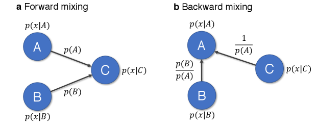
S2-3 Forward mixing of ensembles
Suppose that a virtual ensemble is a mixture of two observable ensembles and by following relation
| (S11) |
where is a probability which represents a ensemble , and is a probability to choose ensemble . If one draws samples from the ensemble and from , the number of samples of is . Thus, in the asymptotic limit of , and . We describe the virtual ensemble as a statistical mixture of two observable ensembles and . We call this description as forward mixing of ensembles. The forward mixing is depicted in Fig. S1. a.
We call one of significant properties of the forward mixing as functional equivalence: expectation of an arbitrary function by the virtual ensemble can be decomposed into those by the observable ensembles and . In other words,
| (S12) |
where . This is a key property to show the asymptotic normality of MLEOQ.
To prove the functional equivalence, we analyze the fluctuation of number count for an outcome of a data set drawn from an ensemble . For each outcome , the number of count can approximate to mean value with standard deviations in the asymptotic limit as
| (S13) |
Let a grand probability distribution of count numbers be . Each probability respective to a number count follows a binomial distribution . In the asymptotic limit of , the Binomial distribution approximates to a Poisson distribution of mean value . Furthermore, as the average number count increases along with the increase of , the Poisson distribution approximates to a normal distribution . Thus, the grand probability finally approximates to the normal distribution as
This implies that in the asymptotic limit of .
By using the approximation of number count (S13), we show that the number count of virtual ensemble is decomposed of those of and as
| (S14) |
From the relation (S11), we can derive that
where we use for the third step and for the fourth step.
Finally, using the relation (S14), we prove the functional equivalence. For the data set of ensemble , , the expectation of function can be read
| (S15) | |||||
This implies that or, equivalently, in the asymptotic limit of .
S2-4 Backward mixing of ensembles
We can describe the forward mixing in a different view that considers the observable ensemble as a mixture of observable ensemble and virtual ensemble . We call this description as backward mixing of ensembles (see Fig. S1. b). In the backward mixing, we have a reciprocal relation of Eq. (S11),
| (S16) |
The backward mixing preserves the functional equivalence, i.e.,
| (S17) |
In the backward problem, the number count satisfies a reciprocal relation of number counts of Eq. (S14).
| (S18) | |||||
Thus, the functional equivalence becomes
| (S19) | |||||
This implies that and, equivalently, in the asymptotic limit of .
S2-5 Operational quasiprobability as a distribution of ensemble mixtures
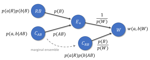
Now we are in a position to interpret the operational quasiprobability (OQ) as a model to represent the forward and backward mixture of ensembles. For the OQ, observable ensembles are , , and , where is a random ensemble, is the ensemble for the single measurement, is the ensemble for the consecutive measurement , and is the marginal ensemble of .
The OQ is obtained by the backward mixing of a virtual ensemble, called , and the marginal ensemble as
| (S20) |
where the virtual ensemble is defined by the forward mixing of observable ensembles and as
| (S21) |
We here consider , , , and , and the OQ in Eq. (S9) is obtained by
| (S22) | |||||
Diagram for the ensemble mixings to construct the OQ is presented in Fig. S2
S2-6 Asymptotic normality of MLEOQ
Based on the aforementioned asymptotic properties, we show that the log-likelihood function of OQ satisfies following three conditions:
Note that we consider a positive function.
Proof of .—In the asymptotic limit of , the second order derivative of log-likelihood function of OQ can be read
where Fisher information of is defined by .
Proof of .—By the functional equivalence in Eq. (S15) and Eq. (S19), can be decomposed into the respective expectations of observable ensembles and in the asymptotic limit of as
By the condition , each term in the right-hand side is zero. Thus, is zero.
Proof of .— We use the condition to prove the condition :
The conditions and imiply that the MLEOQ is unbiased estimator:
| (S23) |
The and imply that MLEOQ is an efficient estimator as
| (S24) |
Thus, the MLEOQ satisfies the asymptotic normality, i.e.,
| (S25) |
Based on these facts, to estimate the estimation error in the asymptotic limit of , we employ an estimator for Fisher information [54, 55] defined by
| (S26) |
Fig. S3 shows that, in a large sample size, the estimation of error closes to the theoretical predictions. In this Figure, we demonstrate the contextuality-enabled enhancement for and estimation. We apply a systematic error model to make the theoretical predictions. Explanation for the error model is presented in the next section.
S3 Error and noise analysis
S3-1 Systematic error model
We characterize systematic errors of our optical setting. The errors do not make our quantum system to lose its coherence, but they cause unwanted drift in experimental results. However, it is impossible to avoid misalignment of control parameters in experiment, so that one performs experiment by allowing a small amount of systematic errors. For example, the axes of wave-plates can be deviated degrees in their alignment.
To anlyze the effect of systematic error, we model a quantum probe state with Bloch representation as
| (S27) |
where satisfying and . For an element of POVM of a binary outcome , we use the representation including biasedness and unsharpness of outcome, which is given by
| (S28) |
where for , and the condition for the measurement to be a POVM is [56]. We also represent overall drift of measurement parameters with a linear model
| (S29) |
where and represent shift of parameters, and and represent scaling of parameters. Finally, a probability obtained by the probe state and the measurement model is given by
| (S30) | |||||
where we abbreviate the model parameters as and .
Our goal is to find the model parameters that best describe the experiments. We collect empirical frequencies for each outcome for a set of states with a priori probability . By Bayes’ theorem, the joint probability is given by
| (S31) |
A uniform distribution for the parameters of quantum state is defined by as . In terms of and , the uniform distribution comes to another distribution . This distribution on continuous space and approximates to the distribution on discrete lattices of as
| (S32) |
where is the index pair to the lattices and . Here, is a normalization constant,
| (S33) |
for the lattice of . We use . With the a priori distribution on the discrete lattice, our model for the joint probability becomes
| (S34) |
To estimate the parameter of measurement model that best describes the experimental results for each lattice point , we use Bayesian inference. We define a log-likelihood function as
| (S35) | |||||
where and . An estimate is a value to give an extremum of log-likelihood function . We assume that the probabilities given by the model is a baseline. In this case, finding an extreme value of likelihood function becomes maximizing Kullback–Leibler divergence , which is defined by
| (S36) |
The is zero if the experimental frequency is equivalent to the model probability . The two approaches result in the same extreme value as
| (S37) | |||||
As the coQM utilizes the two measurements and , we collect empirical frequencies for each measurement, and consider a minimization problem to analyze the systematic errors:
| (S38) |
In summary, we characterize the measurements and with the model parameters and , where meaning of each parameter is following;
:overall drift of
:overall drift of
:scaling factor of
:scaling factor of
:biasedness of measurement ,
:sharpness of measurement ,
:shift of for measurement ,
:shift of for measurement ,
The parameter values for the ideal (no error) case and for an exemplary case with sample size are shown in the table 1. We apply these model parameters to make the theoretical prediction in Fig. S3.
| No error | ||||||||||||
|---|---|---|---|---|---|---|---|---|---|---|---|---|
| Experiment |
S3-2 Effect of depolarization noise
We investigate how performance of contextual quantum metrology depends on purity of a probe state. Depolarization noise degrades coherence of a quantum system, so it is severe error to the quantum system. We represent a partially depolarized quantum state as
| (S39) |
where is a pure probe state, s are Pauli matrices, and indicates degree of purity. for a pure state and for a fully depolarized state , where is an identity matrix. To model the outcome probabilities of partially depolarized state , we mix probabilities obtained by measuring the states and with a measurement as
| (S40) |
where is the probability obtained by measuring the state .
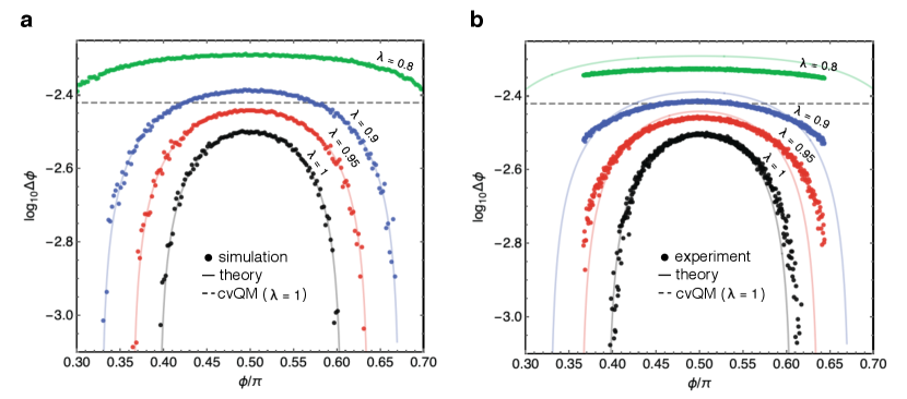
For estimation, we investigate how the estimation error changes by varying from to . Monte-Carlo simulation (Fig. S4 a) shows the degradation of the estimation precision by the depolarization. The gray dashed line is the minimum error in the conventional quantum metrology (cvQM) obtained by the pure probe state. In experiment (Fig. S4 b), we assume that our probe states are pure. We observe the contextuality-enabled enhancement if , and . If , the enhancement is disappeared in the range of the parameters we consider.