XX Month, XXXX \reviseddateXX Month, XXXX \accepteddateXX Month, XXXX \publisheddateXX Month, XXXX \currentdateXX Month, XXXX \doiinfoXXXX.2022.1234567
This work was partially supported by JSPS Grants-in-Aid (23K22762). \authornote This work has been submitted to the IEEE for possible publication. Copyright may be transferred without notice, after which this version may no longer be accessible.
Continuous Relaxation of Discontinuous Shrinkage Operator: Proximal Inclusion and Conversion
Abstract
We present a principled way of deriving a continuous relaxation of a given discontinuous shrinkage operator, which is based on a couple of fundamental results. First, the image of a point with respect to the “set-valued” proximity operator of a nonconvex function is included by that for its lower semicontinuous (l.s.c.) 1-weakly-convex envelope. Second, the “set-valued” proximity operator of a proper l.s.c. 1-weakly-convex function is converted, via double inversion, to a “single-valued” proximity operator which is Lipschitz continuous. As a specific example, we derive a continuous relaxation of the discontinuous shrinkage operator associated with the reversely ordered weighted (ROWL) penalty. Numerical examples demonstrate potential advantages of the continuous relaxation.
convex analysis, proximity operator, weakly convex function
1 Introduction
Triggered by the seminal work [1, 2] of waveshrink by Donoho and Johnstone in 1994, the soft and hard shrinkage operators have been studied in the context of sparse modeling [3, 4], which has a wide range of signal processing applications such as magnetic resonance imaging, radar, sparse coding, compressed sensing/sampling, signal dimensionality reduction, to name just a few [5]. The soft shrinkage operator is characterized as the proximity operator of the norm, where the proximity operator of a convex function is nonexpansive (Lipschitz continuous with unity constant) in general. Because of this, it has widely been used in the operator splitting algorithms [6, 7, 8]. The hard shrinkage operator, on the other hand, is “discontinuous”, while it causes no extra bias in the estimates of large-magnitude coefficients. Hard shrinkage is derived from the set-valued proximity operator of the pseudo-norm.
The firm shrinkage operator [9] has been proposed in 1997, possessing a good balance in the sense of (i) being Lipschitz continuous (with constant strictly greater than unity) and (ii) yielding nearly unbiased estimates of the large-magnitude coefficients. It is the (generalized) proximity operator of the minimax concave (MC) penalty [10, 11] which is weakly convex. Owing to this property, the proximal forward-backward splitting algorithm employing firm shrinkage has a guarantee of convergence to a global minimizer of the objective function [12, 13].
Another discontinuous shrinkage operator has been proposed in the context of image restoration based on the reversely ordered weighted (ROWL) penalty [14], which gives small (possibly zero) weights to dominant coefficients to avoid underestimation so that edge sharpness and gradation smoothness of images are enhanced simultaneously. The ROWL shrinkage operator requires no knowledge about the “magnitude” of the dominant coefficients but instead it requires the “number” of those dominant components essentially. This is in sharp contrast to firm shrinkage which requires (at least a rough approximation, or a sort of bound of) the “magnitude” of the dominant coefficients but it does not care about the “number”. This implies that ROWL shrinkage would be preferable in such situations where the magnitude of dominant components tends to change but the number (or at least its rough estimate) can be assumed to be known a priori. Despite this potential benefit, the ROWL shrinkage operator is discontinuous on the boundaries where some of the components share the same magnitude, provided that the corresponding weights are different. A natural question would be the following: is it possible to convert the discontinuous operator to a continuous one?
To address the above question, our arguments in the present study rely on our recent result [13]: a given operator is the “single-valued” proximity operator of a -weakly convex function for if and only if it is a monotone Lipschitz-continuous gradient (MoL-Grad) denoiser (i.e., it can be expressed as a Lipschitz-continuous gradient operator of a differentiable convex function). See Fact 5. It has been shown in [13] that the operator-regularization approach (or the plug-and-play method [15]) employing a MoL-Grad denoiser actually solves a variational problem involving a weakly convex regularizer which is characterized explicitly by the denoiser.
In this paper, we present a pair of fundamental findings concerning the “set-valued” proximity operator111The “set-valued” proximity operator has been studied previously in the literature [16, 17]. See also [18]. of (proper) nonconvex function, aiming to build a way of converting a discontinuous operator to its continuous relaxation. First, given a nonconvex function, the image of a point with respect to the proximity operator is included by its image with respect to the proximity operator of its lower-semicontinuous 1-weakly-convex envelope (Theorem 1). This well explains the known fact that hard shrinkage can also be derived from the proximity operator of a certain weakly convex function [19, 20], as elaborated in Section 4-4.1. Second, the “set-valued” proximity operator of a (proper) lower-semicontinuous 1-weakly-convex function can be converted, via double inversion, to a MoL-Grad denoiser (Theorem 2). Those proximal inclusion and conversion lead to a principled way of deriving a continuous relaxation (a Lipschitz-continuous relaxation, more specifically) of a given discontinuous operator. As an illustrative example, we show that the firm shrinkage operator is obtained as a continuous relaxation of the hard shrinkage operator. Under the same principle, we derive a continuous relaxation of the ROWL shrinkage operator. Numerical examples show that the continuous relaxation has potential advantages over the original discontinuous shrinkage.
2 Preliminaries
Let be a real Hilbert space with the induced norm . Let , , , and denote the sets of real numbers, nonnegative real numbers, strictly positive real numbers, and nonnegative integers, respectively.
2.1 Lipschitz Continuity of Operator, Set-valued Operator
Let denote the identity operator on . An operator is Lipschitz continuous with constant (or -Lipschitz continuous for short) if
| (1) |
Let denote the power set (the family of all subsets) of . An operator is called a set-valued operator, where for every . Given a set-valued operator , a mapping such that for every is called a selection of . The inverse of a set-valued operator is defined by , which is again a set-valued operator in general.
An operator is monotone if
| (2) |
where gra is the graph of . The following fact is known [21, Proposition 20.10].
Fact 1 (Preservation of monotonicity)
Let be a real Hilbert space, and be monotone operators, be a bounded linear operator, and be a nonnegative constant. Then, the operators , , and are monotone, where denotes the adjoint operator of .
A monotone operator is maximally monotone if no other monotone operator has its graph containing gra properly.
2.2 Lower Semicontinuity and Convexity of Function
A function is proper if the domain is nonempty; i.e., . A function is lower semicontinuous (l.s.c.) on if the level set is closed for every . A function is convex on if for every . For , we say that is -weakly convex if is convex. Here, (i.e., is convex) means that is -strongly convex. Clearly, -weak convexity of implies -weak convexity of for an arbitrary . When the “minimal” weak-convexity parameter is , is nonconvex for every , i.e., is not weakly convex (for any parameter in ). The set of all proper l.s.c. convex functions is denoted by .
Given a proper function , the Fenchel conjugate (a.k.a. the Legendre transform) of is . The conjugate of is called the biconjugate of . In general, is l.s.c. and convex [21, Proposition 13.13].222 It may happen that . For instance, the conjugate of is for every . If , or equivalently if possesses a continuous affine minorant333 Function has a continuous affine minorant if there exist some such that for every ., then is proper and ; otherwise for every [21, Proposition 13.45]. Here, is the l.s.c. convex envelope of .444 The l.s.c. convex envelope is the largest l.s.c. convex function such that , .
Fact 2 (Fenchel–Moreau Theorem [21])
Given a proper function , the following equivalence and implication hold: .
Fact 3
Let be proper. Then, the following statements hold.
2.3 Proximity Operator of Nonconvex Function
Definition 1 (Proximity operator [18, 17])
Let be proper. The proximity operator of of index is then defined by
| (4) |
which is set-valued in general.
We present a slight extension of the previous result [13, Lemma 1] below.
Lemma 1
Let be a proper function. Then, given every positive constant , it holds that
| (5) |
which is monotone.
Proof.
Definition 2 (Single-valued proximity operator [13])
If is single-valued, it is denoted by , which is referred to as the s-prox operator of of index .
As a particular instance, if for some constant , existence and uniqueness of minimizer is automatically ensured. In the convex case of , reduces to the classical Moreau’s proximity operator [22].
Fact 5 ([13] MoL-Grad Denoiser)
Let . Then, for every , the following two conditions are equivalent.555 The case of is due to [22].
-
(C1)
for some such that .
-
(C2)
is a -Lipschitz continuous gradient of a (Fréchet) differentiable convex function . In other words, is a monotone -Lipschitz-continuous gradient (of a differentiable function).
If (C1), or equivalently (C2), is satisfied, then it holds that .
3 Proximal Inclusion and Conversion
Suppose that a given discontinuous (monotone) operator is a selection of the (set-valued) proximity operator of some proper function. Then, there exists a principled way of constructing a continuous relaxation of which is the s-prox operator of a certain weakly convex function. This is the main claim of this article that will be supported by the key results — proximal inclusion and conversion. Some other results on set-valued proximity operators are also presented. All results (lemma, propositions, theorems, corollaries) in what follows are the original contributions of this work.
3.1 Interplay of Maximality of Monotone Operator and Weak Convexity of Function
Fact 5 presented above gives an interplay between -weakly convex functions for and the -Lipschitz continuous gradients of smooth convex functions, stemming essentially from the duality between strongly convex functions and smooth convex functions. Now, the question is the following: is there any such relation in the case of ?
While the proximity operator is (Lipschitz) continuous in the case of , the case of (more specifically, the case in which for any ) includes those functions of which the “set-valued” proximity operator contains a discontinuous shrinkage operator as its selection. The following proposition concerns the case of , which will be linked to the case of later in Section 3-3.2.
Proposition 1
Given a set-valued operator , the following statements are equivalent.
-
1.
for some convex function .
-
2.
for some .
Moreover, if statements 1 – 2 are true, it holds that .
Proof.
The equivalence 1) 2) can be verified by showing the following equivalence basically:
(Proof of ) The last equality can be verified by Lemma 1, and follows by Fact 2.
(Proof of ) Letting , we have again by Fact 2 so that . ∎
Proposition 1 bridges the subdifferential of convex function and the proximity operator of 1-weakly convex function, indicating an interplay between maximality of monotone operators and 1-weak convexity of functions.
Remark 1 (Role of Monotonicity)
From Proposition 1 together with Fact 4.1, implies that is maximally monotone. Viewing the proposition in light of Rockafeller’s cyclic monotonicity theorem [21, Theorem 22.18], moreover, one can see that with if and only if is maximally cyclically monotone.666 An operator is cyclically monotone if, for every integer , for and imply . It is maximally cyclically monotone if no other cyclically monotone operator has its graph containing gra properly [21]. An operator is maximally cyclically monotone if and only if for some (Rockafeller’s cyclic monotonicity theorem). It is clear under Fact 4.1 that a maximally cyclically monotone operator is maximally monotone; the converse is (true when but) not true in general. In words, maximal cyclic monotonicity characterizes the property that can be expressed as the proximity operator (which is set-valued in general) of a 1-weakly convex function. Note that, whereas the proximity operator of a 1-weakly convex function is maximally monotone, the converse is not true in general; i.e., “maximal monotonicity” itself does not ensure that can be expressed as the proximity operator of a 1-weakly convex function.
In Fact 5, monotonicity plays a role of ensuring the convexity of . Indeed, the assumption on in Fact 5 (i.e., the condition for MoL-Grad denoiser) implies maximal cyclic monotonicity, since -weak convexity for implies 1-weak convexity. The assumption required for is actually even stronger than maximal cyclic monotonicity (which is required for ).
3.2 Proximal Inclusion
We start with the definition of the l.s.c. 1-weakly-convex envelope.
Definition 3 (L.s.c. 1-weakly-convex envelope)
Let be a proper function such that is proper as well. Then, is the l.s.c. 1-weakly-convex envelope of . The notation will be used to denote the l.s.c. 1-weakly-convex envelope, such as . The envelope is the largest (proper) l.s.c. 1-weakly-convex function such that , .
The first key result is presented below.
Theorem 1 (Proximal inclusion)
Let be a proper function such that is proper as well. Then, the following inclusion holds between the proximity operators of and its l.s.c. 1-weakly-convex envelope :
| (7) |
i.e., .
Proof.
Theorem 1 implies that, if a discontinuous operator is a selection of for a nonconvex function , it can also be expressed as a selection of for a 1-weakly-convex function , which actually coincides with the l.s.c. 1-weakly-convex envelope of . This fact indicates that, when seeking for a shrinkage operator as (a selection of) the proximity operator, one may restrict attention to the class of weakly convex functions.
We remark that Theorem 1 is trivial if , because in that case by Fact 2. Hence, our primary focus in Theorem 1 is on -weakly convex functions for , although Theorem 1 itself has no such a restriction. The following corollary is a direct consequence of Fact 5 (), Proposition 1 (), and Theorem 1 ().
Corollary 1
Let for . Then, the following statements hold.
-
1.
If , is maximally cyclically monotone. In particular, if , the proximity operator is single valued, and is -Lipschitz continuous.
-
2.
If (more specifically, if ), cannot be maximally cyclically monotone, as for every , provided that is proper.
Remark 2 (On Theorem 1)
3.3 Proximal Conversion
The second key result presented below gives a principled way of converting the set-valued proximity operator of 1-weakly convex function to a MoL-Grad denoiser.
Theorem 2 (Proximal conversion)
Let be a function such that . Then, the proximity operator of the -weakly convex function for the relaxation parameter can be expressed as
| (9) |
which is -Lipschitz continuous.
Proof.
Remark 3
3.4 Surjectivity of Mapping and Continuity of Its Associated Function
An interplay between surjectivity of an operator and continuity (under weak convexity) of a function can be seen through a ‘lens’ of proximity operator.777 It is known that convexity of implies continuity of when is finite dimensional [21, Corollary 8.40].
Lemma 2
Let be a proper function. Then, the following two statements are equivalent.
-
1.
.
-
2.
is convex and continuous over .
Proof.
1) 2): By [21, Proposition 16.5] and Fact 2, it holds that . Hence, invoking [21, Propositions 16.4 and 16.27], we obtain .
2) 1): Clear from [21, Proposition 16.17(ii)]. ∎
Proposition 2
Let be a proper l.s.c. function. Define an operator such that for every . Consider the following two statements.
-
1.
.
-
2.
is convex and continuous.
Then, 1) 2). Assume that ; i.e., has a unique minimizer for every . Then, 1) 2).
4 Application: Continuous Relaxation of Discontinuous Operator
As an illustrative example, we first show how hard shrinkage is converted to a continuous operator by leveraging Theorems 1 and 2. We then apply the same idea to the ROWL-based discontinuous operator to obtain its continuous relaxation.
4.1 An Illustrative Example: Converting Discontinuous Hard Shrinkage to Continuous Firm Shrinkage
The hard shrinkage operator with the threshold is defined by [4]
| (11) |
for which it holds that
| (12) |
where
| (13) |
The l.s.c. 1-weakly convex envelope of is given by (see Fig. 1)
| (14) |
The proximity operator of is given by
| (15) |
where denotes the closed convex hull ( and ). Comparing (12) and (15), it can be seen that
| (16) |
as consistent with Theorem 1. This implies that is also a selection of the proximity operator of the 1-weakly convex function , which is maximally monotone. Indeed, in (15) is the (unique) maximally monotone extension of [20] (cf. Remark 2).
We now invoke Theorem 2 to obtain the continuous operator
| (17) |
where the firm shrinkage operator [9] for the thresholds , , is defined by . We remark that is -weakly convex ( in (17) is -weakly convex) and its “single-valued” proximity operator gives firm shrinkage, while in (16) is 1-weakly convex and a selection of its “set-valued” proximity operator gives hard shrinkage. We also mention that the limit of the continuous operator with respect to the relaxation parameter coincides with the discontinuous operator ; i.e., for every (see Fig. 2).
Fig. 3(a)–(g) illustrates the process of obtaining a continuous relaxation of the discontinuous operator hard1, corresponding to the case of and . Comparing the graphs of the discontinuous operator hard1, , and , one can observe that (see Theorem 1 for the second inclusion)
| (18) |
The maximally monotone operator (see Remark 1) is then converted to in a step-by-step manner using (17) (which is based on Theorem 2). Inspecting the figure under Corollary 1, Figs. 3(b) and 3(h) correspond to Corollary 1.2 (not maximally monotone) for and , respectively, and Figs. 3(c) and 3(g) correspond to Corollary 1.1 (maximally monotone) for and , respectively.
Letting , (17) for concerns the case of . In the case of , on the other hand, the proximity operator of the -weakly convex function is set-valued. Actually, it is not difficult to verify that for every . Note here that this is not true for , i.e., , as can be seen from Figs. 3(b) and 3(c). See Fig. 3(h) for the case of .
4.2 eROWL Shrinkage: Continuous Relaxation of ROWL Shrinkage Operator
We have seen that the discontinuous hard shrinkage operator is converted to the continuous firm shrinkage operator via the transformation from (i) to (vi) in Fig. 3(a). We mimic this procedure for another discontinuous operator.
We consider the Euclidean case for . Let be the weight vector such that . Given , we define of which the th component is given by . Let denote a sorted version of in the nonincreasing order; i.e., . The reversely ordered weighted (ROWL) penalty [14] is defined by . The penalty is nonconvex and thus not a norm.888If , the function is convex, and it is called the ordered weighted (OWL) norm [23].
In this case, the associated proximity operator will be discontinuous. This implies in light of Fact 5 that is not even weakly convex. To see this, let us consider the case of , and let . In this case, by symmetry, the proximity operator is given by , where is the componentwise signum function, denotes the Hadamard (componentwise) product, and for
| (19) |
Here, , and is the ‘ramp’ function. A selection of will be referred to as ROWL shrinkage.
Note that the set in (19) is discrete. This is similar to the case of in (12). Thus, resembling the relation between and corresponding to (i) and (ii) of Fig. 3(a), respectively, we replace the discrete set to its closed convex hull999 For a set , its closed convex hull is given by . . This replacement yields the set-valued operator , where for
| (20) |
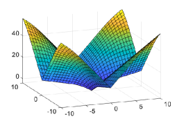
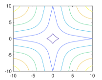
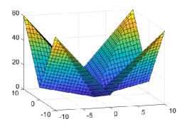
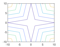
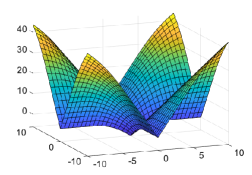
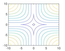
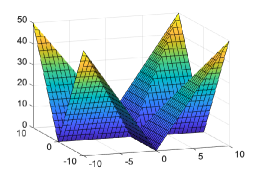
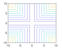
As expected, it can be shown that for the 1-weakly convex function101010One may add to to make the minimum value be zero. (see Figs. 4 and 5)
where with , , and .
We now derive the extended ROWL (eROWL) shrinkage operator by resembling the relation between and corresponding to (ii) and (vi) of Fig. 3, respectively. The eROWL shrinkage operator for the relaxation parameter is defined by
| (21) |
which is -Lipschitz continuous (see Theorem 2). It can readily be verified that , which gives the geometric interpretation shown in Fig. 6. Using this, we can verify that , where, for ,
| (30) |
Here, , for ,
| (31) |
is a triangle given by the intersection of three halfspaces
and
| (32) |
is an unbounded set given by the intersection of the hyperslab and the halfspace
| (33) | ||||
| (34) |
For every , it holds that , where over . An arbitrary selection of the set-valued operator jointly satisfies (i) range and (ii) . This gives a counterexample where in Proposition 2. (The same applies to a selection of .) On the other hand, it holds that range , as consistent with Proposition 2. The operator is a MoL-Grad denoiser; this is a direct consequence of Theorem 2 and Fact 5.
Corollary 2
For every , can be expressed as the ()-Lipschitz continuous gradient of a differentiable convex function.
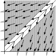
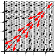
Figure 7 depicts how each point on is mapped by the operators, where the dotted line on the diagonal is the set of ’s with . In the case of ROWL, the mapping is discontinuous on the ‘border’ of the diagonal line. The discontinuity may cause difficulty in analysing convergence when the operator is used in the splitting algorithms. In the case of , the displacement vector on the ‘border’ is aligned with , and it changes continuously when moves away from there gradually.
Remark 4
The eROWL shrinkage operator given in (30) can be represented with another set of parameters and , in place of and . Comparing (20) and (30) under this representation, one can see that of (eROWL) corresponds to (the weight vector of ), and it will therefore be fair to set the weight vectors in a way that . The parameter gives the bound of in the definition of given in (33).
5 Numerical Examples: Sparse Signal Recovery
We consider the simple linear model , where is the sparse (or weakly sparse) signal, is the measurement matrix, and is the i.i.d. Gaussian noise vector. To recover the signal , we consider the iterative shrinkage algorithm in the following form:
| (35) |
where is the shrinkage operator (hard, firm, soft, ROWL, or eROWL), and is the squared-error function with the step size parameter . Clearly, the function is -strongly convex with -Lipschitz continuous gradient for and . As an evaluation metric, we adopt the system mismatch .
5.1 Hard Shrinkage versus Firm Shrinkage
We compare the performance of the “discontinuous” hard shrinkage operator with its continuous relaxation which is firm shrinkage. For comparison, we also test soft shrinkage. The signal of dimension is generated as follows: the first components are generated from the i.i.d. standard Gaussian distribution , and the other components are generated from i.i.d. . The matrix is generated also from . We study the impacts of the parameter of firm shrinkage and the threshold of soft/hard shrinkage on the performance. Although and can be tuned within the range given in [13, Theorem 2], those parameters are set systematically to and for (see Appendix 8). The step size of soft/hard shrinkage is set to . The results are averaged over 20,000 independent trials.
Figure 8 depicts the results for three different sparsity levels , 10, 20 under , 200 and the signal-to-noise ratio (SNR) dB. Table 1 summarizes the reduction rate (gain) of firm shrinkage against hard/soft shrinkage. Thanks to the continuous relaxation, firm shrinkage gains 19.5–44.9 % against hard shrinkage. Compared to soft shrinkage, the gain is 5.3–37.9 %.
5.2 ROWL Shrinkage versus eROWL Shrinkage
The operator is Lipschitz continuous with constant (see Theorem 2), where . To exploit [13, Theorem 2], let . Then, the sequence generated by (35) converges to a minimizer (if exists) of , provided that (a) () and (b) . Thus, unless otherwise stated, we set and with the additional parameters and fixed to and . In the following, eROWL shrinkage is compared to ROWL shrinkage as well as firm shrinkage, where in (35) is replaced by those other shrinkage operators.
| against hard shrinkage | against soft shrinkage | |
|---|---|---|
| case (a) | 41.1 38.5 28.7 | 29.5 25.1 12.1 |
| case (b) | 35.9 32.4 24.8 | 37.9 35.3 20.8 |
| case (c) | 36.2 44.9 41.5 | 25.1 37.9 32.3 |
| case (d) | 19.5 24.7 24.9 | 5.3 32.5 31.8 |
5.2.1 Illustrative Examples
Unlike the continuous eROWL shrinkage , ROWL shrinkage is discontinuous and its corresponding iterate has no guarantee of convergence. To illuminate the potential issue, we consider the noiseless situation (i.e., ) with the matrix (i.e., ) for and the sparse signal . In this case, , . For the sake of illustration, the step size is set to for both ROWL and eROWL, the weight vector of ROWL is set to , and the weight vector of eROWL is chosen, for fairness, in such a way that with (see Remark 4). The convergence for eROWL is guaranteed for every . The algorithms are initialized to .
Figure 9 plots the points , where , , is the intermediate vector between and . The arrows in red color depict the displacement vectors visualizing how each shrinkage operator works. In view of (19), the displacement vector for ROWL is given by basically, guiding the estimate toward a wrong direction. The ROWL iterate converges numerically to , failing to identify the active component. In sharp contrast, the eROWL iterate converges to , identifying the active component correctly. This is because the vector governing the displacement vector depends on the position of the current estimate. More precisely, since the estimate at the early phase is located in the neighborhood of the diagonal (where ), we have , which allows the estimate to be updated toward . We emphasize that this notable advantage comes from the continuity of the eROWL shrinkage operator .
5.2.2 ROWL versus eROWL
We first compare the performance of ROWL and eROWL with the matrix generated randomly from i.i.d. for and with i.i.d. zero-mean Gaussian . For reference, soft shrinkage and firm shrinkage as well as the least squares (LS) estimate, are also tested. Two types of signal are considered: (i) (deterministic) and (ii) (stochastic) with generated randomly from . The results are averaged over 500,000 independent trials.
Figures 10 and 11 depict the results of the deterministic case and the stochastic case, respectively. In Figs. 10(a) and 11(a), the performance for different SNRs is plotted, where the weights of ROWL and eROWL are set to with the second weight is tuned individually by grid search under SNR 20 dB. The threshold of soft shrinkage and of firm shrinkage are also tuned individually under SNR 20 dB. It can be seen that eROWL preserves good performance over the whole range, while the performance curves of soft, firm, and ROWL saturate as SNR increases.
It should also be mentioned that, in the stochastic case, the performance of firm for low SNRs is nearly identical to that of LS. This is because the threshold must fit the magnitude of the active component of but this is difficult in this case as the magnitude changes at every trial randomly. In sharp contrast, eROWL only depends on the “number” of active component (but not on its “magnitude”), and this is why it performs well. The performance of ROWL for low SNRs is ony slightly better than that of LS because of its discontinuity (see Section 5-5.2.5.2.1). In the deterministic case, although firm and ROWL achieves comparable performance to eROWL under SNR 20 dB for which the parameters of each shrinkage operator are tuned, the performance of those shrinkage operators becomes worse significantly as SNR becomes apart from 20 dB.
Figures 10(b) and 11(b) show the impacts of the tuning parameters (or ) of each shrinkage operator for SNR 20 dB. It clearly shows the stable performance of eROWL which comes from the continuity of the eROWL shrinkage operator. This means that is easy to tune and also that eROWL is expected to be robust against possible environmental changes. In contrast, the performance of ROWL degrades as becomes larger than the best value due to its discontinuity. Note that soft/firm shrinkage for too large threshold level yields the zero solution for which the system mismatch is unity.
6 Conclusion
We presented the principled way of constructing a continuous relaxation of a discontinuous shrinkage operator by leveraging the proximal inclusion and conversion (Theorems 1 and 2). As its specific application, the continuous relaxation of the ROWL shrinkage was derived. Numerical examples showed the clear advantages of firm shrinkage and eROWL shrinkage over hard shrinkage and ROWL shrinkage (the discontinuous counterparts), demonstrating the efficacy of the continuous relaxation. A specific situation was presented where the ROWL shrinkage fails but eROWL shrinkage gives a good approximation of the true solution. The simulation results also indicated the potential advantages of eROWL in terms of simplicity of parameter tuning as well as robustness against environmental changes. Although the present study of eROWL is limited to the two dimensional case, its extension to an arbitrary (finite) dimensional case has been presented in [24], where advantages over ROWL have also been shown. We finally mention that the continuous relaxation approach is expected to be useful also for other nonconvex regularizers such as the one proposed in [25].
References
- [1] D. L. Donoho and I. M. Johnstone, “Ideal spatial adaptation by wavelet shrinkage,” Biometrika, vol. 81, no. 3, pp. 425–455, Sep. 1994.
- [2] D. L. Donoho, I. M. Johnstone, G. Kerkyacharian, and D. Picard, “Wavelet shrinkage: Asymptopia?” J. Royal Statistical Society: Series B (Methodological), vol. 57, no. 2, pp. 301–369, Jul. 1995, (with discussions).
- [3] D. L. Donoho, “De-noising by soft-thresholding,” IEEE Trans. Inform. Theory, vol. 41, no. 3, pp. 613–627, May 1995.
- [4] T. Blumensath and M. Davies, “Iterative thresholding for sparse approximations,” J. Fourier Anal. Appl., vol. 14, pp. 629–654, 2008.
- [5] S. Foucart and H. Rauhut, A Mathematical Introduction to Compressive Sensing. New York: Springer, 2013.
- [6] P. L. Combettes and V. R. Wajs, “Signal recovery by proximal forward-backward splitting,” SIAM Journal on Multiscale Modeling and Simulation, vol. 4, no. 4, pp. 1168–1200, 2005.
- [7] H. H. Bauschke, R. S. Burachik, and D. R. Luke, Eds., Splitting Algorithms, Modern Operator Theory, and Applications. Cham: Switzerland: Springer, 2019.
- [8] L. Condat, D. Kitahara, A. Contreras, and A. Hirabayashi, “Proximal splitting algorithms for convex optimization: A tour of recent advances, with new twists,” SIAM Review, vol. 65, no. 2, pp. 375–435, 2023.
- [9] H.-Y. Gao and A. G. Bruce, “Waveshrink with firm shrinkage,” Statistica Sinica, vol. 7, no. 4, pp. 855––874, 1997.
- [10] C. H. Zhang, “Nearly unbiased variable selection under minimax concave penalty,” The Annals of Statistics, vol. 38, no. 2, pp. 894–942, Apr. 2010.
- [11] I. Selesnick, “Sparse regularization via convex analysis,” IEEE Trans. Signal Process., vol. 65, no. 17, pp. 4481–4494, Sep. 2017.
- [12] I. Bayram, “On the convergence of the iterative shrinkage/thresholding algorithm with a weakly convex penalty,” IEEE Trans. Signal Process., vol. 64, no. 6, pp. 1597–1608, 2016.
- [13] M. Yukawa and I. Yamada, “Monotone Lipschitz-gradient denoiser: Explainability of operator regularization approaches and convergence to optimal point,” 2024, arXiv:2406.04676v2 [math.OC].
- [14] T. Sasaki, Y. Bandoh, and M. Kitahara, “Sparse regularization based on reverse ordered weighted l1-norm and its application to edge-preserving smoothing,” in Proc. IEEE ICASSP, 2024, pp. 9531–9535.
- [15] S. V. Venkatakrishnan, C. A. Bouman, and B. Wohlberg, “Plug-and-play priors for model based reconstruction,” in Proc. IEEE Global Conf. Signal Inf. Process, 2013, pp. 945–948.
- [16] R. Gribonval and M. Nikolova, “A characterization of proximity operators,” Journal of Mathematical Imaging and Vision, vol. 62, pp. 773–789, 2020.
- [17] H. H. Bauschke, W. M. Moursi, and X. Wang, “Generalized monotone operators and their averaged resolvents,” Math. Program., vol. 189, no. 55–74, 2021.
- [18] R. T. Rockafellar and R. J.-B. Wets, Variational Analysis, 3rd ed. Berlin Heidelberg: Springer, 2010.
- [19] M. Kowalski, “Thresholding rules and iterative shrinkage/thresholding algorithm: A convergence study,” in Proc. IEEE ICIP, 2014, pp. 4151–4155.
- [20] I. Bayram, “Penalty functions derived from monotone mappings,” IEEE Signal Process. Lett., vol. 22, no. 3, pp. 265–269, 2015.
- [21] H. H. Bauschke and P. L. Combettes, Convex Analysis and Monotone Operator Theory in Hilbert Spaces, 2nd ed. New York: NY: Springer, 2017.
- [22] J. J. Moreau, “Proximité et dualité dans un espace hilbertien,” Bull. Soc. Math. France, vol. 93, pp. 273–299, 1965.
- [23] X. Zeng and M. A. T. Figueiredo, “The ordered weighted norm: Atomic formulation, projections, and algorithms,” arXiv, 2015, arXiv:1409.4271 [cs.DS].
- [24] T. Okuda, K. Suzuki, and M. Yukawa, “Sparse signal recovery based on continuous relaxation of reversely ordered weighted shrinkage operator,” in Proc. IEICE Signal Processing Symposium, Sapporo: Japan, Dec. 2024.
- [25] C. Wang, Y. Wei, and M. Yukawa, “Dispersed-sparsity-aware LMS algorithm for scattering-sparse system identification,” Signal Processing, vol. 225, 2024.
7 Derivation of for
The representation of is visualized in Fig. A.1. The halfspaces and share the same boundary which is depicted by the blue dotted line, and the boundaries of the hyperslab are depicted by the black dashed lines. Figure A.1(b), specifically, illustrates the case in which touches the and axes. This situation happens when lies between and , and it corresponds to the case of . The point is located on the axis, and its inverse image is a set (the line segment in magenta color). In this case, can be expressed as , and it can also be expressed as .
We rephrase the inclusion relation (see Section 4-4.2)
| (A.1) |
which plays a key role in the derivation. Let for . Then, , in Fig. A.1(b) can be expressed as and , and thus their convex combination is given by
| (A.2) |
for . Since (A.1) implies that
| (A.3) |
we obtain
| (A.4) | ||||
| (A.5) |
Substituting (A.5) into (A.2) yields
| (A.10) |
The halfspaces and are derived from the condition , and comes from .
The expression of for can be derived analogously by using and for .
8 Parameters of Firm Shrinkage
By [13, Theorem 2], the iterate given in (35) converges to the minimizer of under the conditions and (see Fact 5 for the relation between and the given operator ). Since is -Lipschitz continuous, we have . This leads to the condition . To satisfy this inequality, we set for a small constant . In this case, we have , and setting the step size to its lower bound gives .
Explain in detail why the contribution of this manuscript is within the scope of the IEEE Open Journal of Signal Processing
Aims & Scope
The IEEE Open Journal of Signal Processing covers the enabling technology for the generation, transformation, extraction, and interpretation of information. It comprises the theory, algorithms with associated architectures and implementations, and applications related to processing information contained in many different formats broadly designated as signals. Signal processing uses mathematical, statistical, computational, heuristic, and/or linguistic representations, formalisms, modeling techniques and algorithms for generating, transforming, transmitting, and learning from signals.
Discontinuous shrinkage operators have a merit of no estimation bias but lack guarantee of algorithm convergence. This paper presents fundamental results enabling to convert discontinuous operators to continuous ones in a principled manner. This is linked to the recently-established mathematical framework for monotone Lipschitz-gradient operators. The author believes that the presented study will boost the research on those signals/data which involve sparseness, low rankness, and so on.