11email: {subxiaona,shower0512,zqzhan,jiyang}@bupt.edu.cn
Contrastive Conditional Alignment based on Label Shift Calibration for Imbalanced Domain Adaptation
Abstract
Many existing unsupervised domain adaptation (UDA) methods primarily focus on covariate shift, limiting their effectiveness in imbalanced domain adaptation (IDA) where both covariate shift and label shift coexist. Recent IDA methods have achieved promising results based on self-training using target pseudo labels. However, under the IDA scenarios, the classifier learned in the source domain will exhibit different decision bias from the target domain. It will potentially make target pseudo labels unreliable, and will further lead to error accumulation with incorrect class alignment. Thus, we propose contrastive conditional alignment based on label shift calibration (CCA-LSC) for IDA, to address both covariate shift and label shift. Initially, our contrastive conditional alignment resolve covariate shift to learn representations with domain invariance and class discriminability, which include domain adversarial learning, sample-weighted moving average centroid alignment and discriminative feature alignment. Subsequently, we estimate the probability distribution of the target domain, and calibrate target sample classification predictions based on label shift metrics to encourage labeling pseudo-labels more consistently with the distribution of real target data. Extensive experiments are conducted and demonstrate that our method outperforms existing UDA and IDA methods on benchmarks with both label shift and covariate shift. Our code is available at https://github.com/ysxcj-hub/CCA-LSC.
Keywords:
Unsupervised domain adaptation Label shift Covariate shift Long-tailed distribution1 Introduction
Unsupervised Domain Adaptation (UDA) [1, 2, 3, 4] aims to transfer knowledge from labeled source domain to unlabeled target domain. A common scenario in UDA is covariate shift, where the conditional distributions of the labels given the features are the same across domains, i.e., , but the marginal distributions of the features are different, i.e., . Many UDA methods have been proposed to deal with covariate shift, such as distribution matching-based methods [3, 4, 5], which aim to align the feature distributions of the source and target domains by minimizing some distance measure. However, when there exists label distribution shift, i.e. , distribution matching-based methods may suffer from negative transfer. In real-world scenarios, domain adaptation often faces the challenge of both data distribution shift (covariate shift) and label distribution shift (label shift). Moreover, real-world data is usually imbalanced, where some classes are more frequent than others. For example, in the domainnet [6] dataset, the head classes that are abundant in the source domain may be scarce in the target domain. This scenario is referred to as imbalanced domain adaptation (IDA). To enable domain adaptation to cope with such realistic situations, effective IDA algorithms are essential.
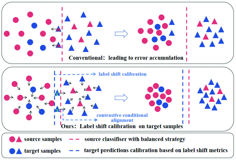
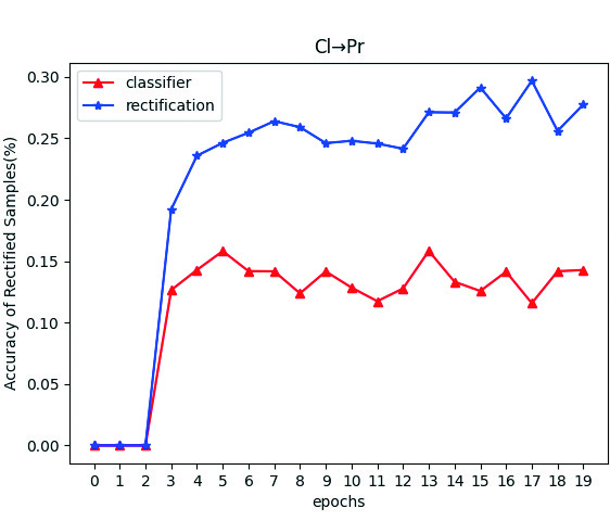
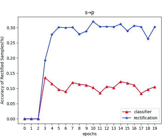
Recent studies attempt to address the IDA problem through self-training with target pseudo-labels. However, these methods prove unstable as the classifier’s output tends to align more closely with the source than the target label distribution under label shift. This discrepancy results in noisier pseudo-labels for target samples. The issue is particularly pronounced for classes with a large label shift, leading to error accumulation, as depicted in Figure 1, top.
To tackle this issue, we introduce a novel method termed contrastive conditional alignment based on label shift calibration (CCA-LSC). This method adjusts the classification of target samples in accordance with the degree of label shift. First, we propose to align the conditional distributions of two domains inspired by contrastive learning by using domain adversarial learning, sample-weighted moving average centroid alignment, and discriminative feature alignment. We then estimate the label distribution of the target domain () after a simple pre-training. Second, we utilize and the label distribution of the source domain to calculate the degree of label shift. Finally, we adjust the classification prediction of target samples according to the degree of label shift during the training process. Our experiments reveal that the pseudo-labels procured by CCA-LSC consistently outperform the pseudo-labels obtained directly from the classifier’s output. This observation, confirmed across all tasks on the OfficeHome and DomainNet datasets, suggests that this strategy effectively enhances the reliability of pseudo-labels, thereby promoting a more accurate alignment across the two domains. See Figure 1, bottom.
The contributions of this article are as follows:
-
•
Contrastive conditional alignment (CCA) leverages the principles of contrastive learning for extracting domain-invariant and class-discriminative features to resist covariate shift. And it weights samples to reduce misalignment from unreliable target pseudo labels.
-
•
Label shift calibration (LSC) introduce a novel metric to quantify label shift and leverage this metric to rectify the classification predictions of target samples, which reduce target false pseudo-rate and resist label shift. CCA and LSC jointly resolve the IDA problem.
-
•
Experiments were conducted on the OfficeHome and DomainNet datasets, which have both label shift and covariate shift, and it was shown that CCA-LSC achieved state-of-the-art performance.
2 Related Work
2.0.1 Unsupervised Domain Adaptation With Covariate Shift
Covariate shift in UDA is primarily addressed by three kind of methods: statistic divergence alignment, adversarial training, and self-training. Statistic divergence alignment learns invariant features by minimizing domain discrepancy, with the divergence measure selection being key. Measures such as maximum mean discrepancy (MMD) [2, 4, 7, 8], correlation alignment [3], wasserstein distance [9, 10, 11], marginal discrepancy measures [12], and other distance-based methods [13, 14] are commonly employed. Adversarial training, taking inspiration from generative adversarial networks (GANs) [15], aims to extract domain invariant features [5, 16, 17, 18] through an adversarial process. These UDA methods align the marginal distribution during training, assuming invariant label distributions. However, label shifts could lead to bad performance or even negative transfer. Self-training [19, 20, 21] employs pseudo-labels generated from the target domain for training on target domain data. However, these pseudo-labels may suffer from miscalibrated probabilities [22], potentially leading to the errors accumulation.
2.0.2 Unsupervised Domain Adaptation With Label Shift
These techniques strive to tackle the challenge of varying label distributions across domains. Predominant strategies include class-weighting methods [23, 24, 25] and those that address cross-domain label shift by predicting and estimating the distribution of the target label [23, 26]. However, these methods presume the feature distribution is invariant across domains, only concentrating on label shift. Additional methods have investigated DA scenarios where the label spaces across domains do not entirely overlap, such as open set domain adaptation [27, 28] and partial domain adaptation [29, 30, 31]. These methods pertain to specific label shift problems, which are not the focus of this paper.
2.0.3 Imbalanced Domain Adaptation
IDA is designed to tackle the coexistence of covariate shift and label shift. Typical methods include conditional distribution alignment based on pseudo-labels [32, 33], class-weighting strategies [34, 35], implicit alignment methods based on sampling [36], asymmetric relaxed distribution alignment [37], and cluster-level discrepancy minimization [38]. These methods typically utilize pseudo-labels for self-training. However, under strong label shift, pseudo-labels are often unreliable, leading to error accumulation and erroneous class alignment. To address this, SENTRY [39] proposed that minimizes the entropy of reliable instances and maximizes the entropy of unreliable instances. ISFDA [40] proposed a method using secondary label correction. However, as label shift varies for different classes, unreliable instances are class-biased. These methods overlook the varying label shift across classes and do not essentially address the label shift issue. In this work, we introduce CCA-LSC. It adjusts the classification prediction of target samples based on each class’s label shift degree, , enhancing the precision of pseudo-labels.
3 Method
3.1 Problem Setup
In this work, we investigated C-way image classification. In imbalanced domain adaptation (IDA), we are given a source domain with labeled samples and a target domain with unlabeled samples , where the input are images and label are categorical variables. For the joint case of label shift and covariate shift, we adopt the same assumption in [32], i.e., , , and . Our goal is to learning a CNN mapping function : .
3.2 Contrastive Conditional Alignment (CCA)
3.2.1 Domain Adversarial Learning
In domain adversarial learning, an auxiliary domain classifier is employed to determine whether the features extracted by are derived from the source or target domain. Simultaneously, is trained to deceive . When this adversarial game reaches a state of equilibrium, the features produced by G demonstrate domain invariance. Formally,
| (1) |
3.2.2 Sample-weighted Moving Average Centroid Alignment
However, domain-invariance does not mean cross domain class-invariance. In [41], they propose to use moving average centroid alignment strategy. This strategy explicitly constrains the distance between centroids with identical class but different domains, ensuring close mapping of same-class features. The transfer objective is:
| (2) |
where and represent the centroid of class of the source and target domains respectively, and represents the Euclidean distance between the two. This strategy is designed to mitigate the adverse effects of incorrect pseudo-labels. However, in situations with severe label shift, an excess of unreliable pseudo-labels can misalign centroids. We suggest that each sample’s contribution to the centroid calculation varies based on its reliability. For instance, in a binary classification problem, if samples and have probability outputs and respectively, is more reliable. Hence, we use confidence as a sample weight. For a sample , the final probability output through a deep model parameterized by is represented as , with a weight of .
3.2.3 Discriminative Feature Alignment
In scenarios with two domains exhibiting significant distribution disparities, our goal is to ensure domain-invariant and class-discriminative features. Features with identical class labels across domains align closely, while those with different labels are distinctly separated. We propose discriminative feature alignment, a contrastive learning-based method, to facilitate this. It computes the difference between each feature pair from the source and target domains, using actual labels for the source and classifier-produced pseudo-labels for the target. Identical class labels draw features closer, while differing labels push them apart, effectively enabling cluster learning for robust classification boundaries. To avoid over-attracting unreliable samples, we persist in using w as a sample weight. Formally,
| (4) |
The above strategies address covariate shift by aligning conditional distributions. However, when class imbalance is present, label shift becomes more pronounced, leading to a biased classifier and impacting the reliability of pseudo-labels. Given the unknown target domain, for generality and simplicity, we employ class-balanced sampling on the source domain. Specifically, when selecting samples for a mini-batch, each class has an equal probability of being selected.
3.3 Label Shift Calibration (LSC)
3.3.1 Label Shift Metrics
Label shift, quantifies the disparity in label distributions between source and target domains. It varies per class due to differing quantity distributions across domains. is defined with respect to the probability distributions and of the source and target domains respectively.
| (5) |
, a tensor, measures label shift, where is the number of classes and represents the label shift degree for class . If , there’s no label shift for class . If , class is more prevalent in the target domain, and if , it’s more prevalent in the source. Both cases indicate label shift, affecting pseudo-label reliability and potentially leading to error accumulation and performance degradation. We derive from source labels. The unlabeled target domain’s is approximated using pseudo-labels, denoted as .
3.3.2 Label Shift Calibration (LSC)
In deep learning classification models, we decompose them into a feature extractor and a classifier . The goal of domain adaptation is to align the features extracted by from two domains. When dealing with long-tailed source data, tends to favor head classes due to their larger quantity, which can lead to suboptimal learning for tail classes with fewer instances. However, even if we adopt class-balanced sampling for the source domain, ensuring an unbiased , the reliability of target sample labeling remains uncertain when the target domain follows a class-imbalanced long-tail distribution. To address this, we propose LSC based on the degree of label shift . LSC calibrates the classification predictions for target samples during training, making the pseudo labels more consistent with the real target data’s probability distribution, thus improving the reliability of target pseudo-labels.
For a target sample through a model with parameters , we use to represent its final probability output. The idea of LSC is to reweight based on the degree of label shift , in order to re-estimate the target pseudo-labels. The class weighting matrix is designed as:
| (6) |
Then we obtain target pseudo labels after calibration and its confidence weight:
| (7) |
| (8) |
A larger suggests that class is less frequent in the source but more so in the target domain, and vice versa for a smaller . As per Eq.6 and Eq.7, when a sample’s feature is on the boundary of two classes and , we prefer to label the sample as , as shown in Figure 1. bounds the class weighting values, with set to 1.5, indicating that only unreliable samples at the classification boundary are calibrated to prevent over-calibration. The sample’s confidence weight is determined by the classifier’s output, mitigating the negative effects of incorrect classification calibration.
3.4 Overall Optimization and Analysis
3.4.1 Overall Optimization
In summary, our training process comprises two stages. The first stage involves pre-training for three epochs, utilizing high-confidence target samples from the training results to estimate the target domain’s label distribution. The optimization objective of the first stage is:
| (9) |
In the second stage, we employ LSC to rectify target pseudo-labels , and utilize for the training of CCA. Then our optimization objective is:
| (10) |
where and and are hyperparameters no less than zero.
3.4.2 Analysis
Next, we demonstrate how our approach reduces the expected error on the target samples from domain adaptation theory.
Theorem 3.1 ( [1])
Denote as the hypothesis. Given two domains and , the target error is bounded by three terms: (i) : source error, (ii) : the discrepancy distance between two distributions S and T, (iii) :shared expected loss. We have:
| (11) |
It is defined as where and are labeling functions for source and target domain respectively. Previous methods often assume that is negligible. However, when is large, ignoring can prevent the learning of an effective target classifier.
Theorem 3.2 ( [41])
In the given formula, the first two terms quantify the discrepancy between the hypothesis and the source labeling function . Given the availability of source labels, these terms are typically minimal, facilitating the learning of a hypothesis space that closely approximates . The third term measures the inconsistency between the source and pseudo-target labeling functions on target samples, while the final term indicates the divergence between the pseudo-target labeling function and the true target label, serving as a reliability measure for the pseudo-labels. Our method seeks to minimize the last two terms to optimize the upper bound of . The moving average centroid alignment strategy, discussed in [41], optimizes the third term by aligning the centroids of target and source features in class , ensuring prediction consistency. Our approach employs both sample-weighted moving average centroid alignment and discriminative feature alignment to foster feature alignment across different domains but within the same class, thereby minimizing the third term.
However, [41] presumes the fourth term will minimize over time and disregards it. This assumption falls short in the presence of data imbalance and label shift, where optimizing the third term could induce class bias in the pseudo-target labeling function, amplifying the fourth term. Our proposed LSC rectifies this by adjusting the classification prediction of the pseudo-target labeling function based on the label shift index , reducing the false pseudo-rate, and aligning the prediction with the true target data’s label distribution, thereby also minimizing the fourth term. Our experiments demonstrate that LSC consistently curtails the false pseudo-rate on target samples (refer to section 4.4).
In essence, the efficacy of domain adaptation methods hinges on managing each term that could escalate the target classification error, thus broadening the applicability of domain adaptation methods.
4 Experiments
4.1 Set up
4.1.1 Datasets
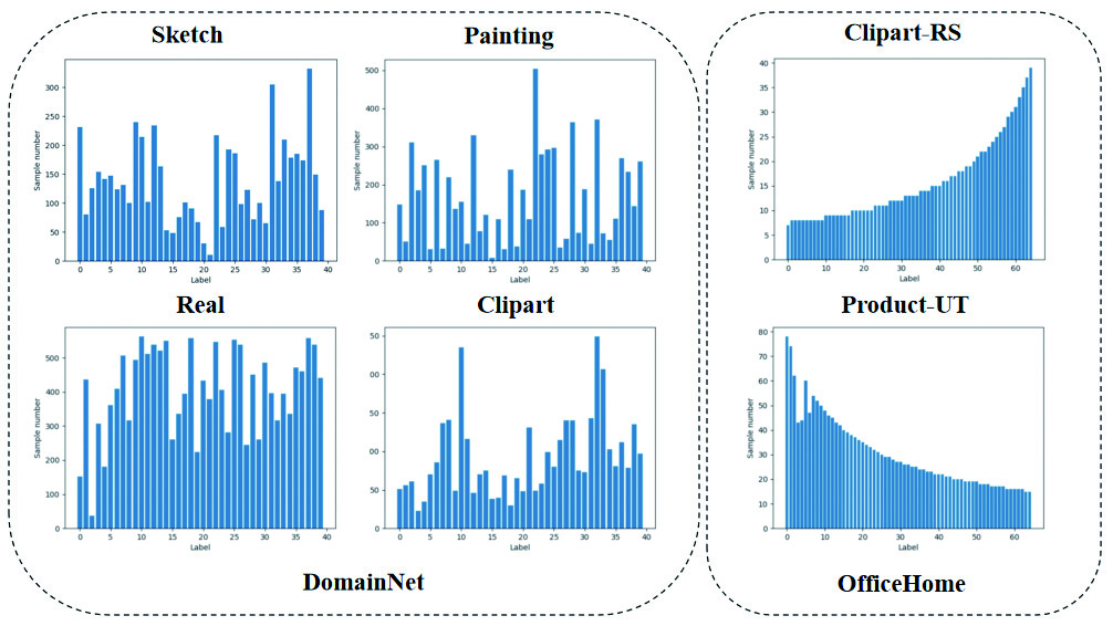
We utilized three datasets . First, we employed Office-Home (RS-UT), an imbalanced version of Office-Home created by [32], where the source and target domains follow two reverse Paredo distributions. This benchmark includes three domains: Clipart (Cl), Product images (Pr), and Real-world images (Rw). The Art images (Ar) domain in Office-Home, being too small for sampling an imbalanced subset, is not considered here. Second, we used a subset of DomainNet created by [32], which includes 40 classes from four domains (Real (R), Clipart (C), Painting (P), Sketch (S)). As a noticeable label shift already exists, we made no additional modifications. The label distributions can be seen in Figure 1. Office-31 [44] contains 4,110 images of 31 categories. The domains are Amazon (A), Webcam (W), and DSLR (D).
4.1.2 Baselines
We benchmarked our method against eight state-of-the-art techniques that tackle both covariate shift and label shift. (i) COAL [32] aligns feature and label distributions using prototype-based conditional alignment and self-training on confident pseudo-labels. (ii) MDD+Implicit Alignment (I.A) [36] removes explicit model parameter optimization from pseudo-labels via sampled implicit alignment. (iii) InstaPBM [45] employs instance-based prediction behavior matching. (iv) F-DANN [37] introduces a DANN based on asymmetric relaxed distribution matching. (v) SENTRY [39] minimizes the entropy of reliable instances and maximizes that of unreliable ones. (vi)TIToK [46] and (vii)BIWAA-I [47] and (viii)RHWD [48] also solve both label and feature shifting problems. All methods, except F-DANN, use target pseudo-labels. We also compared with conventional UDA methods like BBSE [23], which only addresses label shift, and MCD [17], DAN [4], DANN [5], JAN [7], BSP [49], which solely focus on covariate shift.
4.1.3 Implementation details
All experiments are conducted using the Pytorch framework with resnet50. The model’s hyper-parameters are , , and . The bottleneck layer dimension is 256, and the batch size is 50. We use the SGD optimizer with a momentum of 0.9. The initial learning rate for the classifier is 0.005 for OfficeHome and 0.01 for DomainNet, adjusted as [5]. The model trains for 20 epochs, with the first 3 forming the initial stage. After this, the model evaluates target samples and uses pseudo-labels with a confidence level of to estimate the target domain’s label distribution. The model then enters the second stage. The random seed is set to 100 for reproducibility. For imbalanced data, we use per-class mean accuracy, as suggested by [32], for a fair performance assessment.
Methods R→C R→P R→S C→R C→P C→S P→R P→C P→S S→R S→C S→P AVG source 65.75 68.84 59.15 77.71 60.60 57.87 84.45 62.35 65.07 77.10 63.00 59.72 66.80 MCD 61.97 69.33 56.26 79.78 56.61 53.66 83.38 58.31 60.98 81.74 56.27 66.78 65.42 DANN 63.37 73.56 72.63 86.47 65.73 70.58 86.94 73.19 70.15 85.73 75.16 70.04 74.46 F-DANN 66.15 71.80 61.53 81.85 60.06 61.22 84.46 66.81 62.84 81.38 69.62 66.50 69.52 JAN 65.57 73.58 67.61 85.02 64.96 67.17 87.06 67.92 66.10 84.54 72.77 67.51 72.48 BSP 67.29 73.47 69.31 86.50 67.52 70.90 86.83 70.33 68.75 84.34 72.40 71.47 74.09 COAL 73.85 75.37 70.50 89.63 69.98 71.29 89.81 68.01 70.49 87.97 73.21 70.53 75.89 MDD+I.A 78.54 75.09 69.43 88.50 70.59 70.44 88.37 75.71 71.65 89.35 77.97 72.41 77.33 InstaPBM 80.10 75.87 70.84 89.67 70.21 72.76 89.60 74.41 72.19 87.00 79.66 71.75 77.84 SENTRY 83.89 76.72 74.43 90.61 76.02 79.47 90.27 82.91 75.60 90.41 82.40 73.98 81.39 BIWAA-I 79.93 75.24 75.35 87.93 72.07 75.71 88.87 77.81 76.66 88.78 80.49 74.49 79.44 RHWD [48] 84.80 76.90 75.20 91.80 75.60 81.20 91.90 84.60 76.10 91.30 83.20 74.60 82.00 Ours 83.74 77.10 79.00 90.21 76.54 78.55 89.62 81.86 79.57 90.49 83.06 77.48 82.27
Methods RwPr RwCl PrRw PrCl ClRw ClPr AVG source 70.74 44.24 67.33 38.68 53.51 51.85 54.39 BBSE 61.10 33.27 62.66 31.15 39.70 38.08 44.33 MCD 66.03 33.17 62.95 29.99 44.47 39.01 45.94 DAN 69.35 40.84 66.93 34.66 53.55 52.09 52.90 DANN 71.62 46.51 68.40 38.07 58.83 58.05 56.91 F-DANN 68.56 40.57 67.32 37.33 55.84 53.67 53.88 JAN 67.20 43.60 68.87 39.21 57.98 48.57 54.24 COAL 73.65 42.58 73.26 40.61 59.22 57.33 58.40 MDD+I.A 76.08 50.04 74.21 45.38 61.15 63.15 61.67 InstaPBM 75.56 42.93 70.30 39.32 61.87 63.40 58.90 SENTRY 76.12 56.80 73.60 54.75 65.94 64.29 65.25 TIToK 77.09 52.84 72.15 44.32 60.06 59.95 61.07 Ours 79.18 60.53 78.26 50.13 65.79 68.99 67.15
Methods AW DW WD AD DA WA AVG DAN 68.5 96.0 99.0 67.0 54.0 53.1 72.9 DANN 82.0 96.9 99.1 79.7 68.2 67.4 82.2 MCD 88.6 98.5 100. 92.2 69.5 69.7 86.5 MDD 94.5 98.4 100. 93.5 74.6 72.2 88.9 BIWAA-I 95.6 99.0 100. 95.4 75.9 77.3 90.5 Ours 96.0 99.1 100. 94.6 77.1 77.3 90.7
4.2 Results
DomainNet and OfficeHome.
The experimental results on DomainNet and OfficeHome are presented in Tables 2 and 2, respectively. Our method outperforms the second best method SENTRY, by improving the average accuracy by 1.90% on OfficeHome (RS-UT) and by 0.88% on DomainNet. Table 2 reveals that our method significantly surpasses SENTRY in scenarios with higher label shifts, such as RS, PS, and SP, registering increases of 4.57%, 3.97%, and 3.50%, respectively. Table 2 shows a better promotion since there are severe label shift. These results highlight our method’s efficacy in simultaneously tackling label shift and covariate shift.
Office-31.
The experimental results are shown in Tables 3. There are few label shifts but feature shifts in this dataset. It can be seen that our method also has good performance for solving the problem of feature shifting.
Different Degrees of Label Shift.
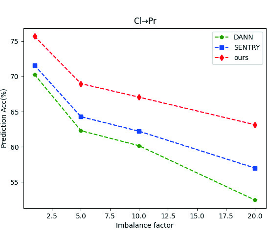
We measure imbalance using the imbalance factor IF [50], defined as the ratio of maximum to minimum class sizes. A larger IF indicates more imbalance. We created four splits on ClPr with IF. For IF=1, we used the original Cl and Pr data from OfficeHome. For other splits, we maintained the maximum class size and adjusted the Pareto distribution parameters based on OfficeHome (RS-UT). All methods used class-balanced sampling in the source domain for fairness. As shown in Figure 2, accuracy decreases for all methods with increasing imbalance due to label shift, but our method consistently outperforms the others.
4.3 Ablation Study
To mitigate the influence of source data imbalance, we evaluated each domain adaptation component using class-balanced sampling on the source domain. Table LABEL:ablation presents the results. Model performance is bad with only source cross-entropy loss. Performance improves with the addition of adversarial learning and sample-weighted moving average centroid alignment loss (+). Significant improvement is observed with the inclusion of discriminative feature alignment loss (), which ensures both domain invariance and class discriminability of the learned representation. Label shift calibration on target samples further enhances performance by reducing the target false pseudo rate during training, ensuring correct execution of the two pseudo label-based strategies.
| 1 | 1.5 | 2 | |
|---|---|---|---|
| ClPr | 68.32 | 68.99 | 68.44 |
| 0.4 | 0.6 | 0.8 | |
|---|---|---|---|
| 1 | 67.18 | 67.73 | 68.06 |
| 3 | 68.22 | 68.99 | 68.34 |
| 5 | 68.56 | 68.11 | 67.16 |
4.4 Analysis of Label Shift Calibration
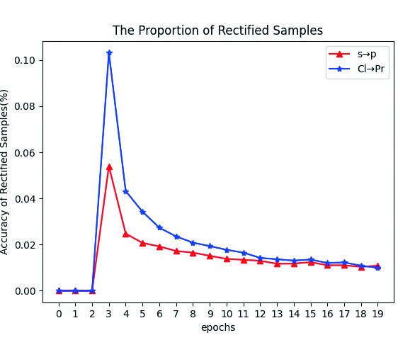
The label shift calibration strategy calibrates only some target pseudo labels at the classification boundary, leading to two scenarios: consistency () and inconsistency () between the classifier’s output pseudo labels and the calibrated ones. Figure 2 illustrates the proportion of samples with calibrated pseudo labels () during training, which decreases over time, indicating an increasing number of samples moving away from the classification boundary. Figures 2 and 2 show the right proportion of and in these calibrated samples. During the initial 3 epochs of pre-training, label shift calibration is not applied. Throughout the training, the accuracy of consistently surpasses that of , demonstrating the strategy’s effectiveness in reducing the false pseudo rate of the classifier’s target output, supporting the analysis in Section 3.4. In fact, higher accuracy of over , was observed in all 18 transfer tasks on OfficeHome and DomainNet during training.
A question naturally arises: given the label shift between source and target domains, could we diminish this shift by implementing pseudo-label balanced sampling on the target domain and class-balance sampling on the source domain? Initially, the balanced sampling strategy curbs imbalance by regulating the utilization of input data, inevitably leading to an over-sampling of certain classes. This is more likely to negatively impact the quality of the learned representation for unlabeled target domain data. Furthermore, our application of pseudo-label balanced sampling on the OfficeHome dataset resulted in a reduction of per-class accuracy by about 1%. Consequently, we have decided not to use pseudo-label balanced sampling strategy on target data in our method.
4.5 Hyper-parameter Discussion
The Influence of the Parameter .
The dictates the proportion of calibrated samples. A smaller value leads to a larger proportion of . Although our calibration strategy is effective, more calibrations aren’t always better. Over-calibration can lead to over-representation of the dominant class in target samples, while under-calibration can lessen its effectiveness. Table 6 illustrates the impact of the . To counteract the effects of incorrect calibrations, we derive the confidence of all target pseudo labels from the classifier’s probability output. For instance, if a sample’s probability output is [0.6, 0.4] and the calibrated output is [0.45, 0.55], its confidence is 0.4 and its weight . This can effectively reduce the adverse impact of incorrect calibrations.
Hyper-parameter Analysis.
We fixed to 1 and discussed the impact of and . The experimental results are shown in the Table 6. It can be seen that our experimental results are not sensitive to each hyperparameter.
4.6 Analysis of Two Stage Learning
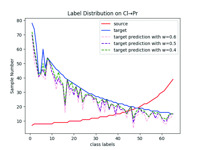
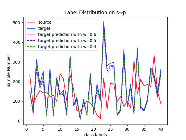
Our LSC strategy relies on the distribution estimation of the target domain in the first stage. When this estimation is highly unreliable, the LSC strategy may fail. Therefore, we discuss the impact of the pre-training of CCA in the first stage on the LSC strategy in the second stage. Figure 3 shows the results of estimating the target domain distribution by selecting pseudo-labels of target samples with different confidence levels. It can be seen that when the confidence level , , , our estimated distribution of the target domain is generally close to its true distribution, indicating that is reliable. In fact, our estimation of the target domain distribution does not need to be very accurate, as long as it can generally reflect the target label distribution. In our experiments, we use pseudo-labels of target samples with a confidence level of to estimate the target domain distribution.
5 Conclusion
We introduce CCA-LSC to tackle label shift and covariate shift in imbalanced domain adaptation. Our approach employs domain adversarial learning, sample-weighted moving average centroid alignment, and discriminative feature alignment for contrastive conditional alignment, facilitating the learning of feature representations that are both domain-invariant and class-discriminative. To counter label shift, we introduce the label shift measure , using it to calibrate the classification prediction of target samples. Experimental evidence demonstrates that CCA-LSC delivers state-of-the-art results on benchmark datasets.
Acknowledgements.
The paper is supported by the National Natural Foundation Science of China (62101061).
References
- [1] Ben-David S, Blitzer J, Crammer K, et al. A theory of learning from different domains[J]. Machine learning, 2010, 79: 151-175.
- [2] Long M, Zhu H, Wang J, et al. Unsupervised domain adaptation with residual transfer networks[J]. Advances in neural information processing systems, 2016, 29.
- [3] Sun B, Saenko K. Deep coral: Correlation alignment for deep domain adaptation[C]//Computer Vision–ECCV 2016 Workshops: Amsterdam, The Netherlands, October 8-10 and 15-16, 2016, Proceedings, Part III 14. Springer International Publishing, 2016: 443-450.
- [4] Long M, Cao Y, Wang J, et al. Learning transferable features with deep adaptation networks[C]//International conference on machine learning. PMLR, 2015: 97-105.
- [5] Ganin Y, Ustinova E, Ajakan H, et al. Domain-adversarial training of neural networks[J]. Journal of machine learning research, 2016, 17(59): 1-35.
- [6] Peng X, Bai Q, Xia X, et al. Moment matching for multi-source domain adaptation[C]//Proceedings of the IEEE/CVF international conference on computer vision. 2019: 1406-1415.
- [7] Long M, Zhu H, Wang J, et al. Deep transfer learning with joint adaptation networks[C]//International conference on machine learning. PMLR, 2017: 2208-2217.
- [8] Ge P, Ren C X, Xu X L, et al. Unsupervised domain adaptation via deep conditional adaptation network[J]. Pattern Recognition, 2023, 134: 109088.
- [9] Balaji Y, Chellappa R, Feizi S. Normalized wasserstein for mixture distributions with applications in adversarial learning and domain adaptation[C]//Proceedings of the IEEE/CVF International Conference on Computer Vision. 2019: 6500-6508.
- [10] Lee J, Raginsky M. Minimax statistical learning with wasserstein distances[J]. Advances in Neural Information Processing Systems, 2018, 31.
- [11] Shen J, Qu Y, Zhang W, et al. Wasserstein distance guided representation learning for domain adaptation[C]//Proceedings of the AAAI conference on artificial intelligence. 2018, 32(1).
- [12] Zhang Y, Liu T, Long M, et al. Bridging theory and algorithm for domain adaptation[C]//International conference on machine learning. PMLR, 2019: 7404-7413.
- [13] Li J, Jing M, Lu K, et al. Locality preserving joint transfer for domain adaptation[J]. IEEE Transactions on Image Processing, 2019, 28(12): 6103-6115.
- [14] Li J, Jing M, Su H, et al. Faster domain adaptation networks[J]. IEEE Transactions on Knowledge and Data Engineering, 2021, 34(12): 5770-5783.
- [15] Goodfellow I, Pouget-Abadie J, Mirza M, et al. Generative adversarial nets[J]. Advances in neural information processing systems, 2014, 27.
- [16] Long M, Cao Z, Wang J, et al. Conditional adversarial domain adaptation[J]. Advances in neural information processing systems, 2018, 31.
- [17] Saito K, Watanabe K, Ushiku Y, et al. Maximum classifier discrepancy for unsupervised domain adaptation[C]//Proceedings of the IEEE conference on computer vision and pattern recognition. 2018: 3723-3732.
- [18] Rangwani H, Aithal S K, Mishra M, et al. A closer look at smoothness in domain adversarial training[C]//International conference on machine learning. PMLR, 2022: 18378-18399.
- [19] Mei K, Zhu C, Zou J, et al. Instance adaptive self-training for unsupervised domain adaptation[C]//Computer Vision–ECCV 2020: 16th European Conference, Glasgow, UK, August 23–28, 2020, Proceedings, Part XXVI 16. Springer International Publishing, 2020: 415-430.
- [20] Wei C, Shen K, Chen Y, et al. Theoretical analysis of self-training with deep networks on unlabeled data[J]. arXiv preprint arXiv:2010.03622, 2020.
- [21] Zou Y, Yu Z, Liu X, et al. Confidence regularized self-training[C]//Proceedings of the IEEE/CVF international conference on computer vision. 2019: 5982-5991.
- [22] Guo C, Pleiss G, Sun Y, et al. On calibration of modern neural networks[C]//International conference on machine learning. PMLR, 2017: 1321-1330.
- [23] Lipton Z, Wang Y X, Smola A. Detecting and correcting for label shift with black box predictors[C]//International conference on machine learning. PMLR, 2018: 3122-3130.
- [24] Azizzadenesheli K, Liu A, Yang F, et al. Regularized learning for domain adaptation under label shifts[J]. arXiv preprint arXiv:1903.09734, 2019.
- [25] Azizzadenesheli K. Importance weight estimation and generalization in domain adaptation under label shift[J]. IEEE Transactions on Pattern Analysis and Machine Intelligence, 2021, 44(10): 6578-6584.
- [26] Alexandari A, Kundaje A, Shrikumar A. Maximum likelihood with bias-corrected calibration is hard-to-beat at label shift adaptation[C]//International Conference on Machine Learning. PMLR, 2020: 222-232.
- [27] Panareda Busto P, Gall J. Open set domain adaptation[C]//Proceedings of the IEEE international conference on computer vision. 2017: 754-763.
- [28] Yang X, Deng C, Liu T, et al. Heterogeneous graph attention network for unsupervised multiple-target domain adaptation[J]. IEEE Transactions on Pattern Analysis and Machine Intelligence, 2020, 44(4): 1992-2003.
- [29] Cao Z, Ma L, Long M, et al. Partial adversarial domain adaptation[C]//Proceedings of the European conference on computer vision (ECCV). 2018: 135-150.
- [30] Zhang J, Ding Z, Li W, et al. Importance weighted adversarial nets for partial domain adaptation[C]//Proceedings of the IEEE conference on computer vision and pattern recognition. 2018: 8156-8164.
- [31] Zhang Y, Ji J C, Ren Z, et al. Digital twin-driven partial domain adaptation network for intelligent fault diagnosis of rolling bearing[J]. Reliability Engineering & System Safety, 2023, 234: 109186.
- [32] Tan S, Peng X, Saenko K. Class-imbalanced domain adaptation: An empirical odyssey[C]//Computer Vision–ECCV 2020 Workshops: Glasgow, UK, August 23–28, 2020, Proceedings, Part I 16. Springer International Publishing, 2020: 585-602.
- [33] Tachet des Combes R, Zhao H, Wang Y X, et al. Domain adaptation with conditional distribution matching and generalized label shift[J]. Advances in Neural Information Processing Systems, 2020, 33: 19276-19289.
- [34] Wang J, Chen Y, Hao S, et al. Balanced distribution adaptation for transfer learning[C]//2017 IEEE international conference on data mining (ICDM). IEEE, 2017: 1129-1134.
- [35] Yan H, Ding Y, Li P, et al. Mind the class weight bias: Weighted maximum mean discrepancy for unsupervised domain adaptation[C]//Proceedings of the IEEE conference on computer vision and pattern recognition. 2017: 2272-2281.
- [36] Jiang X, Lao Q, Matwin S, et al. Implicit class-conditioned domain alignment for unsupervised domain adaptation[C]//International conference on machine learning. PMLR, 2020: 4816-4827.
- [37] Wu Y, Winston E, Kaushik D, et al. Domain adaptation with asymmetrically-relaxed distribution alignment[C]//International conference on machine learning. PMLR, 2019: 6872-6881.
- [38] Yang J, Yang J, Wang S, et al. Advancing imbalanced domain adaptation: Cluster-level discrepancy minimization with a comprehensive benchmark[J]. IEEE Transactions on Cybernetics, 2021.
- [39] Prabhu V, Khare S, Kartik D, et al. Sentry: Selective entropy optimization via committee consistency for unsupervised domain adaptation[C]//Proceedings of the IEEE/CVF International Conference on Computer Vision. 2021: 8558-8567.
- [40] Li X, Li J, Zhu L, et al. Imbalanced source-free domain adaptation[C]//Proceedings of the 29th ACM international conference on multimedia. 2021: 3330-3339.
- [41] Xie S, Zheng Z, Chen L, et al. Learning semantic representations for unsupervised domain adaptation[C]//International conference on machine learning. PMLR, 2018: 5423-5432.
- [42] Crammer K, Kearns M, Wortman J. Learning from Multiple Sources[J]. Journal of Machine Learning Research, 2008, 9(8).
- [43] Hjelm R D, Fedorov A, Lavoie-Marchildon S, et al. Learning deep representations by mutual information estimation and maximization[J]. arXiv preprint arXiv:1808.06670, 2018.
- [44] Saenko K, Kulis B, Fritz M, et al. Adapting visual category models to new domains[C]//Computer Vision–ECCV 2010: 11th European Conference on Computer Vision, Heraklion, Crete, Greece, September 5-11, 2010, Proceedings, Part IV 11. Springer Berlin Heidelberg, 2010: 213-226.
- [45] Li B, Wang Y, Che T, et al. Rethinking distributional matching based domain adaptation[J]. arXiv preprint arXiv:2006.13352, 2020.
- [46] Wang Y, Chen Q, Liu Y, et al. TIToK: A solution for bi-imbalanced unsupervised domain adaptation[J]. Neural Networks, 2023, 164: 81-90.
- [47] Westfechtel T, Yeh H W, Meng Q, et al. Backprop induced feature weighting for adversarial domain adaptation with iterative label distribution alignment[C]//Proceedings of the IEEE/CVF winter conference on applications of computer vision. 2023: 392-401.
- [48] Si L, Dong H, Qiang W, et al. Regularized hypothesis-induced wasserstein divergence for unsupervised domain adaptation[J]. Knowledge-Based Systems, 2024, 283: 111162.
- [49] Chen X, Wang S, Long M, et al. Transferability vs. discriminability: Batch spectral penalization for adversarial domain adaptation[C]//International conference on machine learning. PMLR, 2019: 1081-1090.
- [50] Cui Y, Jia M, Lin T Y, et al. Class-balanced loss based on effective number of samples[C]//Proceedings of the IEEE/CVF conference on computer vision and pattern recognition. 2019: 9268-9277.