Contrastive explainable clustering with differential privacy

Dung Nguyen , Ariel Vetzler ¹¹footnotemark: 1 , Sarit Kraus ³³footnotemark: 3 , Anil Vullikanti ²²footnotemark: 2 These authors contributed equally. Correspondence to: Dung Nguyen (dungn@virginia.edu)Department of Computer Science, and Biocomplexity Institute and Initiative, University of Virginia, USADepartment of Computer Science, Bar-Ilan University, Israel

Abstract

This paper presents a novel approach in Explainable AI (XAI), integrating contrastive explanations with differential privacy in clustering methods. For several basic clustering problems, including $k$ -median and $k$ -means, we give efficient differential private contrastive explanations that achieve essentially the same explanations as those that non-private clustering explanations can obtain. We define contrastive explanations as the utility difference between the original clustering utility and utility from clustering with a specifically fixed centroid. In each contrastive scenario, we designate a specific data point as the fixed centroid position, enabling us to measure the impact of this constraint on clustering utility under differential privacy. Extensive experiments across various datasets show our method’s effectiveness in providing meaningful explanations without significantly compromising data privacy or clustering utility. This underscores our contribution to privacy-aware machine learning, demonstrating the feasibility of achieving a balance between privacy and utility in the explanation of clustering tasks.

1 Introduction

Different notions of clustering are fundamental primitives in several areas, including machine learning, data science, and operations research Reddy (2018). Clustering objectives (e.g., $k$ -median and $k$ -means), crucial in facility location planning, have been notably applied in pandemic response strategies, such as determining optimal sites for COVID-19 vaccination and testing centers Bertsimas et al. (2022); Mehrab et al. (2022). The distance to a cluster center becomes a significant factor in these scenarios, particularly highlighted during the COVID-19 pandemic, where accessible vaccine locations played a pivotal role Rader et al. (2022). This context often leads to individuals, especially those distant from a cluster center, seeking explanations for their specific assignment or location in the clustering plan. For example, consider a resident questioning why a COVID-19 testing center isn’t located next to their home. Such queries reflect the need for explainability in clustering decisions, where factors like population density, resource allocation, and public health considerations impact site selection. The resident’s inquiry underscores the importance of transparent methodologies in clustering that can provide understandable explanations for facility placements, especially in critical health scenarios.

Such questions fall within the area of Explainable AI, which is a rapidly growing and vast area of research Finkelstein et al. (2022); Sreedharan et al. (2020); Miller (2019); Boggess et al. (2023). We focus on post-hoc explanations, especially contrastive explanations, e.g., Miller (2019), which address “why P instead of Q?” questions. Such methods have been used in many applications, including multi-agent systems, reinforcement learning, and contrastive analysis, e.g., Boggess et al. (2023); Sreedharan et al. (2021); Madumal et al. (2020); Sreedharan et al. (2020). In the context of the clustering problems mentioned above, a possible explanation for a resident is the increase in the cost of the clustering if a center is placed close to the resident, compared to the cost of an optimal solution, which is relatively easy to compute. This increased cost reflects a trade-off, where optimizing for one resident’s convenience could result in worse centroid positions for other residents, highlighting the complex decision-making process in clustering for fair resource distribution.

Data privacy is a crucial concern across various fields, and Differential Privacy (DP) is one of the most widely used and rigorous models for privacy Dwork and Roth (2014). We focus on the setting where the set of data points $\mathbf{X}=\{x_{1},\ldots,x_{n}\}$ are private; for instance, in the vaccine center deployment problem, each $x_{i}$ corresponds to an individual who is seeking vaccines, and would like to be private. There has been a lot of work on the design of differentially private solutions to clustering problems like $k$ -median and $k$ -means under such a privacy model Ghazi et al. (2020); Gupta et al. (2010); Balcan et al. (2017); Stemmer and Kaplan (2018). These methods guarantee privacy of the data points $\mathbf{X}$ and output a set of centers $c_{1},\ldots,c_{k}$ (which are public) such that its cost, denoted by $\text{cost}^{p}_{\mathbf{X}}(c_{1},\ldots,c_{k})$ is within multiplicative and additive factors $w$ and $t$ of the optimal solution $OPT_{\mathbf{X}}$ , i.e., $\text{cost}^{p}_{\mathbf{X}}(c_{1},\ldots,c_{k})\leq w\cdot OPT_{\mathbf{X}}+t$ .

While there has been significant progress in various domains of differential privacy, the intersection of explainability and differential privacy still needs to be explored. In clustering problems, a potential private contrastive explanation given to agent $i$ is to provide the $\text{cost}(S^{(i)}_{\epsilon})$ - $\text{cost}(S_{\epsilon})$ , where $S_{\epsilon}$ is a set of centers generated by private algorithm (with privacy budget $\epsilon$ ), and $\text{cost}(S^{(i)}_{\epsilon})$ is the cost of the clustering solution while fixing one center at agent $i$ ’s location. However, giving such a private contrastive explanation to each agent $i$ naively using a $(w,t)$ -approximate private clustering would lead to $(w,t\sqrt{n}/\epsilon)$ -approximation, even if we use advanced composition techniques for privacy. The central question of our research: is it possible to offer each user a private contrastive explanation with a limited overall privacy budget?

Our contributions.

1. We introduce the PrivEC problem, designed to formalize private contrastive explanations to all agents in clustering using $k$ -median and $k$ -means objectives.
2. We present an $\epsilon$ -DP mechanism, PrivateExplanations, which provides a contrastive explanation to each agent while ensuring the same utility bounds as private clustering in Euclidean spaces Ghazi et al. (2020). We use the private coreset technique of Ghazi et al. (2020), which is an intermediate private data structure that preserves similar clustering costs as the original data. The main technical challenge is to derive rigorous bounds on the approximation factors for all the contrastive explanations.
3. We evaluate our methods empirically on realistic datasets used in the problems of vaccine center deployment in Virginia Mehrab et al. (2022). Our results show that the privacy-utility trade-offs are similar to those in private clustering, and the errors are quite low even for reasonable privacy budgets, demonstrating the effectiveness of our methods.

Our research stands out by seamlessly integrating differential privacy into contrastive explanations, maintaining the quality of explanations even under privacy constraints. This work bridges the gap between privacy and explainability, marking a significant advancement in privacy-aware machine learning. Due to space limitations, we present many technical details and experimental evaluations in the Appendix.

2 Related Work

Our work considers differential privacy for explainable AI in general (XAI) and Multi-agent explanations (XMASE) in particular, focusing on post-hoc contrastive explanations for clustering. We summarize some of the work directly related to our paper; additional discussion is presented in the Appendix, due to space limitations.

Extensive experiments presented in Saifullah et al. (2022) demonstrate non-negligible changes in explanations of black-box ML models through the introduction of privacy.

Nguyen et al. (2023) considers feature-based explanations (e.g., SHAP) that can expose the top important features that a black-box model focuses on. To prevent such expose they introduced a new concept of achieving local differential privacy (LDP) in the explanations, and from that, they established a defense, called XRAND, against such attacks. They showed that their mechanism restricts the information that the adversary can learn about the top important features while maintaining the faithfulness of the explanations.

Goethals et al. (2022) study the security of contrastive explanations, and introduce the concept of the “explanation linkage attack”, a potential vulnerability that arises when employing strategies to derive contrastive explanations. To address this concern, they put forth the notion of k-anonymous contrastive explanations. As the degree of privacy constraints increases, a discernible trade-off comes into play: the quality of explanations and, consequently, transparency are compromised.

Closer to our application is the work of Georgara et al. (2022), which investigates the privacy aspects of contrastive explanations in the context of team formation. They present a comprehensive framework that integrates team formation solutions with their corresponding explanations, while also addressing potential privacy concerns associated with these explanations. Additional evaluations are needed to determine the privacy of such heuristic-based methods.

There has been a lot of work on private clustering and facility location, starting with Gupta et al. (2010), which was followed by a lot of work on other clustering problems in different privacy models, e.g., Huang and Liu (2018); Stemmer (2020); Stemmer and Kaplan (2018); Nissim and Stemmer (2018); Feldman et al. (2017). Gupta et al. (2010) demonstrated that the additive error bound for points in a metric space involves an $O(\Delta k^{2}\log{n}/\epsilon)$ term, where $\Delta$ is the space’s diameter. Consequently, all subsequent work, including ours, assumes points are restricted to a unit ball.

We note that our problem has not been considered in any prior work in the XAI or differential privacy literature. The formulation we study here will likely be useful for other problems requiring private contrastive explanations.

3 Preliminaries

Let $\mathbf{X}\subset\mathbb{R}^{d}$ denote a dataset consisting of $d$ -dimensional points (referred to sometimes as agents). We consider the notion of $(k,p)$ -clustering, as defined by Ghazi et al. (2020).

Definition 1.

( $(k,p)$ -Clustering Ghazi et al. (2020)). Given $k\in\mathbb{N}$ , and a multiset $\mathbf{X}=\{x_{1},\ldots,x_{n}\}$ of points in the unit ball, a $(k,p)$ -clustering is a set of $k$ centers $\{c_{1},\ldots,c_{k}\}$ minimizing $\text{cost}^{p}_{\mathbf{X}}(c_{1},\ldots,c_{k})=\sum_{i\in[n]}\min_{j\in[k]}\|x_{i}-c_{j}\|^{p}$ .

For $p=1$ and $p=2$ , this corresponds to the $k$ -median and $k$ -means objectives, respectively. We drop the subscript $\mathbf{X}$ and superscript $p$ , when it is clear from the context, and refer to the cost of a feasible clustering solution $S$ by $\text{cost}(S)$ .

Definition 2.

( $(w,t)$ -approximation). Given $k\in\mathbb{N}$ , and a multiset $\mathbf{X}=\{x_{1},\ldots,x_{n}\}$ of points in the unit ball, let $OPT^{p,k}_{\mathbf{X}}=\min_{c_{1},\ldots,c_{k}\in\mathbb{R}^{d}}\text{cost}^{p}_{\mathbf{X}}(c_{1},\ldots,c_{k})$ denote the cost of an optimal $(k,p)$ -clustering. We say $c_{1},\ldots,c_{k}$ is a $(w,t)$ – approximation to a $(k,p)$ -optimal clustering if $\text{cost}^{p}_{\mathbf{X}}(c_{1},\ldots,c_{k})\leq w\cdot OPT^{p,k}_{\mathbf{X}}+t$ .

A coreset (of some original set) is a set of points that, given any $k$ centers, the cost of clustering of the original set is “roughly” the same as that of the coreset Ghazi et al. (2020).

Definition 3.

For $\gamma,t>0,p\geq 1,k,d\in\mathbb{N}$ , a set $X^{\prime}$ is a $(p,k,\gamma,t)$ -coreset of $X\subseteq\mathbb{R}^{d}$ if for every $C=\{c_{1},\ldots,c_{k}\}\in R^{d}$ , we have $(1-\gamma)cost_{X}^{p}(C)-t\leq cost_{X^{\prime}}(C)\leq(1+\gamma)cost_{X}^{p}(C)+t$ .

Privacy model. We use the notion of differential privacy (DP), introduced in Dwork and Roth (2014), which is a widely accepted formalization of privacy. A mechanism is DP if its output doesn’t differ too much on “neighboring” datasets; this is formalized below.

Definition 4.

$\mathcal{M}:\mathcal{X}\to\mathcal{Y}$ is $(\epsilon,\delta)$ -differentially private if for any neighboring datasets $X\sim X^{\prime}\in\mathcal{X}$ and $S\subseteq\mathcal{Y}$ ,

\displaystyle\Pr[\mathcal{M}(X)\in S]\leq e^{\epsilon}\Pr[\mathcal{M}(X^{\prime})\in S]+\delta.

If $\delta=0$ , we say $\mathcal{M}$ is $\epsilon$ -differentially private.

We operate under the assumption that the data points in $\mathbf{X}$ represent the private information of users or agents. We say $\mathbf{X},\mathbf{X}^{\prime}$ are neighboring (denoted by $\mathbf{X}\sim\mathbf{X}^{\prime}$ ) if they differ in one data point. When a value is disclosed to an individual agent $i$ , it is imperative to treat the remaining clients in $\mathbf{X}-\{i\}$ as private entities. To address this necessity, we adopt the following privacy model:

Definition 5.

A mechanism $\mathcal{M}$ is $\epsilon$ - $i$ -exclusive DP if, $\forall X,X^{\prime}:X\setminus\{i\}\sim X^{\prime}\setminus\{i\}$ , and for all $S\subseteq Range(\mathcal{M})$ :

\displaystyle\Pr[\mathcal{M}(X)\in S]\leq e^{\epsilon}\Pr[\mathcal{M}(X^{\prime})\in S].

Note that if $\mathcal{M}$ is $\epsilon$ -DP, it is $\epsilon$ - $i$ -exclusive DP for any $i$ .

Relation to Joint-DP model. Kearns et al. (2014) defines Joint-DP–a privacy model that “for each of agent $i$ , knowledge of the $n-1$ agents does not reveal much about agent $i$ ”. It contrasts with our privacy model, where each explanation to agent $i$ uses direct and private knowledge of agent $i$ (that private knowledge will be returned to only agent $i$ ) and such knowledge does not reveal much about $n-1$ other agents.

In clustering scenarios such as k-means or k-median, it is beneficial for an individual data point to be positioned near the cluster center, as this reduces its distance. This concept has practical applications in fields such as urban planning and public health. For example, clustering algorithms like $k$ -means and $k$ -median have been utilized to optimize the placement of mobile vaccine centers, as noted in Mehrab et al. (2022). However, once the cluster centers are calculated, residents might wonder why a vaccine clinic has not been positioned nearer to their homes. Our objective is to provide explanations for each data point that is not near a cluster center. Following the approach suggested by Miller (2019), one way to provide an explanation is to re-run the clustering algorithm, this time setting the resident’s location as a fixed centroid. This allows us to explain the changes in clustering costs, where an increase could describe why certain placements are less optimal.

The focus of this paper is twofold: residents not only need explanations but also wish to maintain their privacy, preferring not to disclose their precise locations/data publicly. Traditional private clustering methods struggle to offer these private explanations because they accumulate the privacy budget by continuously applying private clustering to answer numerous inquiries, ultimately resulting in explanations that are not private. Thus, we have developed a framework that delivers the necessary explanations to residents while protecting their confidentiality.

In essence, our framework is data-agnostic and capable of offering contrastive explanations for any private data within clustering algorithms, effectively balancing the need for privacy with the demand for transparency in decision-making.

Definition 6.

Private and Explainable Clustering problem (PrivEC) Given an instance $\mathbf{X}\in\mathcal{X}^{n}$ , clustering parameters $k,p$ , and a subset of data points: $V_{s}\subset\mathbf{X}$ , the goal is to output:
Private: An $\epsilon$ -DP clustering solution $S_{\epsilon}$ (available to all)
Explainable: For each $i\in V_{s}$ , output $\text{cost}(S^{(i)}_{\epsilon})$ - $\text{cost}(S_{\epsilon})$ , which is $\epsilon$ - $i$ -exclusive DP.
$S^{(i)}_{\epsilon}$ is a private solution computed by the clustering algorithm while fixing one centroid to the position of agent $i$ .
We assume that $S^{(i)}_{\epsilon}$ is not revealed to any agent, but $\text{cost}(S^{(i)}_{\epsilon})$ - $\text{cost}(S_{\epsilon})$ is released to agent $i$ as contrastive explanation.

4 peCluster Mechanism

The PrivateClustering algorithm Ghazi et al. (2020) includes dimension reduction, forming a private coreset, applying an approximation clustering algorithm on the coreset, and then reversing the dimension reduction, ultimately yielding an $\epsilon$ -DP clustering solution.

The PrivateExplanations algorithm receives the original private clustering cost from PrivateClustering and then leverages the PrivateClustering framework but introduces a fixed-centroid clustering algorithm on the coreset instead of regular approximation clustering algorithm, followed by a dimension reverse. Ultimately, after calculating the fixed centroid clustering algorithm and determining its cost in the original dimension, we subtract the original private clustering cost obtained from the PrivateClustering algorithm, outputting $\text{cost}(S^{(i)}_{\epsilon})$ - $\text{cost}(S_{\epsilon})$ .

To elaborate further, Private Clustering first reduces the dataset’s dimensionality using DimReduction (Algorithm 1) to enable efficient differentially private coreset construction. It then uses a DP Exponential Mechanism to build a PrivateCoreset (Algorithm 7 of Ghazi et al. (2020)), which is clustered using any $w^{\prime\prime}$ -approximate, not necessarily private clustering algorithm. The low-dimensional clustering cost is scaled to obtain the original high-dimensional cost, and the centroids are recovered in the original space. Multiplying the low-dimensional clustering cost with $(\log(n/\beta)/0.01)^{p/2}$ gives the clustering cost of the original high-dimensional instance Makarychev et al. (2019). By Running DimReverse using FindCenter (Algorithm 10 of Ghazi et al. (2020)) we can find the centroids in the original space. The output is the private centroids, their cost, the private coreset, and the low-dimensional dataset. We employed DimReduction since PrivateCoreset is an exponential algorithm. This approach enables the transformation of dimensionality reduction into an exponential process, effectively converting the algorithm’s time complexity from exponential to polynomial with respect to the input size.
The following summarizes Algo. 3 - PrivateClustering:

Input: Agents’ location ( $X$ ), original and reduced dimension (d, d’). Output: Private clustering: centers and cost.

1.

Dimension reduction - Algorithm 1 DimReduction
2.

Private coreset - Algorithm. PrivateCoreset
3.

Clustering on the coreset - Algorithm NonPrivateApprox
4.

Dimension reverse - 2 DimReverse

Algorithm 1 DimReduction
Input:

(x_{1},x_{2},\ldots,x_{n}),d,d^{\prime},\beta

Output:

(x^{\prime}_{1},\ldots,x^{\prime}_{n})

low-dimensional space dataset.

\Lambda=\sqrt{\frac{0.01d}{\log(n/\beta)d^{\prime}}}

2: for

i\in\{1,..,n\}

\tilde{x}_{i}\leftarrow\Pi_{\mathcal{S}}(x_{i})

4: if

\|\tilde{x}_{i}\|\leq 1/\Lambda

then

x^{\prime}_{i}=\Lambda\tilde{x}_{i}

6: else

x^{\prime}_{i}=0

8: end if

9: end for

10: return

(x^{\prime}_{1},\ldots,x^{\prime}_{n})

Algorithm 2 DimReverse
Input:

(c^{\prime}_{1},\ldots,c^{\prime}_{k}),(x^{\prime}_{1},\ldots,x^{\prime}_{n})

Output:

(c_{1},\ldots,c_{k})

Private Centroids in high dimension

\mathbf{X}_{1},\ldots,\mathbf{X}_{k}\leftarrow\text{ the partition induced by }

(c^{\prime}_{1},\ldots,c^{\prime}_{k})

(x^{\prime}_{1},\ldots,x^{\prime}_{n})

2: for

j\in\{1,\ldots,k\}

c_{j}\leftarrow\textsc{FindCenter}^{\epsilon/2}(\mathbf{X}_{j})

4: end for

5: return

(c_{1},\ldots,c_{k})

Algorithm 3 PrivateClustering
Input:

(x_{1},x_{2},\ldots,x_{n}),d,d^{\prime},k,\epsilon,\lambda,p,\alpha,\beta

Output:

(\epsilon,\delta)

-differentially private centers

c_{1,..,k}

with cost

S_{\epsilon}

Y

Private Coreset and

(x^{\prime}_{1},\ldots,x^{\prime}_{n})

low-dimensional space dataset.

\zeta=0.01\left(\frac{\alpha}{10\lambda_{p,\alpha/2}}\right)^{p/2}

(x^{\prime}_{1},\ldots,x^{\prime}_{n})

\leftarrow

DimReduction((x_{1},\ldots,x_{n}),d,d^{\prime},\beta)

Y\leftarrow\textsc{PrivateCoreset}^{\epsilon/2}(x^{\prime}_{1},\ldots,x^{\prime}_{n},\zeta)

((c^{\prime}_{1},\dots,c^{\prime}_{k}),cost(S^{\prime}_{\epsilon}))\leftarrow NonPrivateApprox(Y,k)

cost(S_{\epsilon})=\left(\frac{\log(n/\beta)}{0.01}\right)^{p/2}cost(S^{\prime}_{\epsilon})

c\leftarrow\textsc{DimReverse}^{\epsilon/2}((c^{\prime}_{1},\dots,c^{\prime}_{k}),(x^{\prime}_{1},\dots,x^{\prime}_{n}))

7: return

c=\{c_{1},\ldots,c_{k}\},cost(S_{\epsilon})

Y

(x^{\prime}_{1},\ldots,x^{\prime}_{n})

Algorithm 4 PrivateExplanations
Input:

Y,\text{cost}(S_{\epsilon}),V_{s},k,\epsilon,p,n,\beta

Output: {

cost(S_{\epsilon})-cost(S^{(i)}_{\epsilon}):i\in V_{s}\}

DP explanations for each agent (i)

1: for

i\in V_{s}

cost(S^{(i)}_{\epsilon})\leftarrow\left(\frac{\log(n/\beta)}{0.01}\right)^{\frac{p}{2}}NonPrivateApproxFC(Y,k,x^{\prime}_{i})

3: end for

4: return

\{cost(S_{\epsilon})-cost(S^{(i)}_{\epsilon}):i\in V_{s}\}

Private contrastive explanation:
The following summarizes Algorithm 4 - PrivateExplanations:

Input: Private coreset ( $Y$ ), Private clustering cost ( $cost(S_{\epsilon})$ ), Agents looking for contrastive explanation ( $V_{s}$ ).
Output: Explanation for each agent in $V_{s}$ ( $\text{cost}(S_{\epsilon})-cost(S^{(i)}_{\epsilon}$ )).

1.

Fixed-centroid clustering on Coreset - NonPrivateApproxFC (specifically for $k$ -means and $k$ -median in Section 4.2 and Section 4.1 respectively)
2.

Calculate clustering cost by multiplication - Algorithm 4, line 2.
3.

Return utility decrease as an explanation - Algorithm 4, line 4.

After the completion of PrivateClustering, which yields private centroids, specific users within $V_{s}\subset\mathbf{X}$ , may request an explanation regarding the absence of a facility at their particular location. We want to provide each agent with the overall cost overhead that a facility constraint at his specific location will yield. To address these queries, we integrate our peCluster mechanism. This algorithm takes the previously computed coreset and employs our NonPrivateApproxFC(tailor-suited non-private algorithm we designed and explained in the following sections) $w^{\prime}$ -approximate algorithm to output the cost of $(k,p)$ -clustering with a fixed centroid.

The output of our algorithm provides the difference cost of the clustering, denoted as cost( $S^{(i)}_{\epsilon}$ ) - cost( $S_{\epsilon}$ ). This output effectively captures the contrast between the overall clustering cost and the specific clustering cost when an individual agent ( $i$ ) inquires about the absence of a facility at their location, aligning precisely with the key objectives and functions outlined earlier in the abstract.
The privacy analysis, as demonstrated in Theorem 1, establishes the privacy guarantees of PrivateClustering and peCluster. The output $Y$ is $\epsilon/2$ -differentially private as an output of $\epsilon/2$ -DP algorithm. Consequently, both $(c^{\prime}_{1},\ldots,c^{\prime}_{k})$ and $cost(S_{\epsilon})$ maintain $\epsilon/2$ -DP status, under the Post-Processing property.
Applying $\textsc{DimReverse}^{\epsilon/2}$ to find the centers in the original space, $c=\{c_{1},\ldots,c_{k}\}$ is $\epsilon$ -DP by Composition theorem. For each $i$ , cost( $S^{(i)}_{\epsilon}$ ) is produced by Post-Processing of $Y$ with only $x^{\prime}_{i}$ , hence $cost(S^{(i)}_{\epsilon}$ ) satisfies $\epsilon$ - $i$ -exclusive-DP.

Theorem 1.

(Full proof in Theorem 5.) The solution $(c_{1},\ldots,c_{k})$ and $cost(S_{\epsilon})$ released by Algorithm 3 are $\epsilon$ -DP. For all clients $i$ , the value $S^{(i)}_{\epsilon}$ released by Algorithm 4 is $\epsilon$ - $x_{i}$ -exclusive DP.

A critical component of our algorithm involves a detailed utility analysis. In the following sections, we will present rigorous upper bounds and specific constraints for k-means and k-median.

Utility Analyses. PrivateCoreset is setup with parameter $\zeta$ (other than the privacy budget $\epsilon/2$ ), which depends on $\alpha$ (Line 1, Algorithm 3). It leads to the cost of every clustering on $Y$ (the coreset) is off from its cost on $X^{\prime}$ by a multiplicative factor of $(1+0.1\alpha)$ plus an additive factor of $\overset{\sim}{O}(\text{polylog}(n/\beta)/\epsilon)$ . Then, by applying the Dimensional Reduction lemma (Appendix section B), which states that the cost of a specific clustering on $X^{\prime}$ ( $d^{\prime}$ -dimensional space) is under some constant factor of the same clustering on $X$ ( $d$ -dimensional space), we can bound the $cost({S_{\epsilon}}^{(i)})$ by its optimal clustering $OPT_{i}$ .

Lemma 1.

(Full proof in Lemma 7) With probability at least $1-\beta$ , $S_{\epsilon}$ (clustering cost) is a $(w,t)$ -approximation of $OPT$ , where¹¹1We use the notation $\mathcal{O}_{p,\alpha}$ to explicitly ignore factors of $p,\alpha$ :

	$\displaystyle w$	$\displaystyle=w^{\prime\prime}(1+\alpha),$		(1)
	$\displaystyle t$	$\displaystyle=w^{\prime\prime}\mathcal{O}_{p,\alpha}\left((k/\beta)^{O_{p,\alpha}(1)}.\text{polylog}(n/\beta)/\epsilon\right)$		(2)

We note that $\Lambda$ is chosen carefully by composing (1) the factor of $(d/d^{\prime})^{1/2}$ , which will scale to $(d/d^{\prime})^{p/2}$ due to $\|.\|_{p}$ operator and cancel out the scaling factor $(d^{\prime}/d)^{p/2}$ occurs when mapping the cost of clustering from the lower dimensional space to the original space and (2) the factor of $0.01/\log(n/\beta)$ that guarantees each $\|x^{\prime}_{i}\|<1/\Lambda$ with probability at least $1-0.1\beta/n$ (and for all $i$ simultaneously with probability $1-0.1\beta$ ).

Theorem 2.

(Full proof in Theorem 6) Fix an $i$ . With probability at least $1-\beta$ , $S^{(i)}_{\epsilon}$ released by Algorithm 4 is a $(w,t)$ -approximation of $OPT_{i}$ -the optimal $(k,p)$ -clustering cost with a center fixed at position $x_{i}$ , in which:

	$\displaystyle w$	$\displaystyle=w^{\prime}(1+\alpha)$		(3)
	$\displaystyle t$	$\displaystyle=w^{\prime}\mathcal{O}_{p,\alpha}\left((k/\beta)^{O_{p,\alpha}(1)}.\text{polylog}(n/\beta)/\epsilon\right)$		(4)

Lemma 2.

(Full proof in Lemma 8) Fix an $i$ . If $OPT_{i}\geq w^{\prime\prime}(1+\alpha)OPT+t^{(i)}$ , then with probability at least $1-2\beta$ , ${S_{\epsilon}}$ and ${S_{\epsilon}}^{(i)}$ released by Algorithm 3 and 4 satisfies that ${S_{\epsilon}}^{(i)}>{S_{\epsilon}}$ .

Running Time Analysis. Assume that polynomial-time algorithms exist for $(k,p)$ -clustering and for $(k,p)$ -clustering with a fixed center. Setting $d^{\prime}=O(p^{4}\log(k/\beta))$ (that satisfies Dimension-Reduction-Lemma(Appendix section B)), algorithm PrivateCoreset takes $O(2^{O(d^{\prime})}\text{poly}(n))$ time (Lemma 42 of Ghazi et al. (2020)), which is equivalent to $O((k/\beta)^{O_{p,\alpha}(1)}\text{poly}(n))$ . FindCenter takes $O(\text{poly}(np))$ time (Corollary 54 of Ghazi et al. (2020)) and is being called $k$ times in total. Finally, we run $1$ instance of $(k,p)$ -clustering and $|V_{s}|$ instances of $(k,p)$ -clustering with a fixed center. It follows that the total running time of our algorithm is $O((k/\beta)^{O_{p,\alpha}(1)}\text{poly}(nd))$ . This means the computational complexity of our algorithm is polynomial in relation to the size of the input data.

Tight Approximation Ratios. Corollary 1 and 2 will wrap up this section by presenting a specific, tight approximation ratio( $w^{\prime}$ ) achieved after applying NonPrivateApproxFC. These corollaries will detail and confirm the algorithm’s effectiveness in achieving these approximation ratios.

4.1 NonPrivateApproxFC for $k$ -median

As previously mentioned, we have specifically developed a non-private fixed centroid clustering algorithm, referred to as NonPrivateApproxFC. Our algorithm is proved to be an 8-approximation algorithm. We obtain our results by adapting Charikar et al. (1999) to work with a fixed centroid (Moving forward in our discussion, we will refer to the fixed centroid as $C$ ). To grasp how we adapted the algorithm to suit our needs, it’s essential to understand the definitions used in Charikar et al. (1999) as they introduce demand $d_{j}$ for each location $j\in N$ as a weight reflecting the location’s importance. $N$ represents list of agents ${1\ldots n}$ . For the conventional k-median problem, each $d_{j}$ is initially set to 1 for all $j\in N$ . The term $c_{ij}$ represents the cost of assigning any $i$ to $j$ and $x_{ij}$ represents if location $j$ is assigned to center $i$ .
We first assume that the fixed center is one of the input data points $N$ to formulate the $k$ -median problem with a fixed center as the solution of the integer program (in the Appendix). We can then relax the IP condition to get the following LP:

minimize	$\displaystyle\sum_{i,j\in N}d_{j}c_{ij}x_{ij}$	(5)
$\displaystyle\text{s.t.}\sum_{i\in N}x_{ij}$	$\displaystyle=1\text{ for each $j\in N$};\sum_{j\in N}y_{j}=k$	(6)
$\displaystyle x_{ij}$	$\displaystyle\leq y_{i}\text{ for each $i,j\in N$}$	(7)
$\displaystyle x_{ij},y_{i}$	$\displaystyle\geq 0\text{ for each $i,j\in N$}$	(8)
$\displaystyle y_{C},x_{CC}$	$\displaystyle\geq 1\text{ for a fixed $C\in N$}$	(9)

Let $(\bar{x},\bar{y})$ be a feasible solution of the LP relaxation and let $\bar{C}_{j}=\sum_{i\in N}c_{ij}\bar{x}_{ij}$ for each $j\in N$ as the total (fractional) cost of client $j$ .

The first step. We group nearby locations by their demands without increasing the cost of a feasible solution $(\bar{x},\bar{y})$ , such that locations with positive demands are relatively far from each other. By re-indexing, we get $\bar{C}_{C}\leq\bar{C}_{1}\leq\bar{C}_{2}\leq\ldots\bar{C}_{n}$ .

We will show that it’s always possible to position $\bar{C}_{C}$ as the first element of the list, i.e., $\bar{C}_{C}$ is equal to the minimum value of all $\bar{C}_{j}$ . Recall that: $\bar{C}_{C}=\sum_{i\in N}c_{iC}\bar{x}_{iC}=\sum_{i\in N,i\neq C}c_{iC}\bar{x}_{iC}+c_{CC}\bar{x}_{CC}=0,$ since we know that $\sum_{i\in N}x_{iC}=1,x_{CC}\geq 1$ and $c_{CC}=0$ .

The remaining work of the first step follows Charikar et al. (1999). We first set the modified demands ${d_{j}}^{\prime}\leftarrow d_{j}$ . For $j\in N$ , moving all demand of location $j$ to a location $i<j$ s.t. $d^{\prime}_{i}>0$ and $c_{ij}\leq 4\bar{C}_{j}$ , i.e., transferring all $j$ ’s demand to a nearby location with existing positive demand. Demand shift occurs as follows: $d^{\prime}_{i}\leftarrow d^{\prime}_{i}+d^{\prime}_{j},d^{\prime}_{j}\leftarrow 0$ . Since we initialize $d^{\prime}_{C}=d_{C}=1$ , and we never move its demands away, it follows that $d^{\prime}_{C}>0$ .

Let $N^{\prime}$ be the set of locations with positive demands $N^{\prime}=\{j\in N,d^{\prime}_{j}>0\}$ . A feasible solution to the original demands is also a feasible solution to the modified demands. By Lemma 11, for any pair $i,j\in N^{\prime}$ : $c_{ij}>4\max(\bar{C}_{i},\bar{C}_{j})$ .

Lemma 3.

The cost of the fractional $(\bar{x},\bar{y})$ for the input with modified demands is at most its cost for the original input.

Proof.

The cost of the LP $\bar{C}_{LP}=\sum_{j\in N}d_{j}\bar{C}_{j}$ and $\bar{C}^{\prime}_{LP}=\sum_{j\in N}d^{\prime}_{j}\bar{C}_{j}$ . Since we move the demands from $\bar{C}_{j}$ to a location $i$ with lower cost $\bar{C}_{i}\leq\bar{C}_{j}$ the contribution of such moved demands in $\bar{C}^{\prime}$ is less than its contribution in $\bar{C}$ , it follows that $\bar{C}^{\prime}_{LP}\leq\bar{C}_{LP}$ . ∎

The second step. We analyze the problem with modified demands $d^{\prime}$ . We will group fractional centers from the solution $(\bar{x},\bar{y})$ to create a new solution $(x^{\prime},y^{\prime})$ with cost at most $2\bar{C}_{LP}$ such that $y^{\prime}_{i}=0$ for each $i\notin N^{\prime}$ and $y^{\prime}_{i}\geq 1/2$ for each $i\in N^{\prime}$ . We also ensure that $y^{\prime}_{C}\geq 1/2$ in this step, i.e., $C$ will be a fractional center after this.

The next lemma states that for each $j\in N$ , there are at least $1/2$ of the total fractional centers within the distance of $2\bar{C}_{j}$ .

Lemma 4.

For any $1/2$ -restricted solution $(x^{\prime},y^{\prime})$ there exists a $\{1/2,1\}$ -integral solution with no greater cost.

Proof.

The cost of the $\frac{1}{2}$ -restricted solution (by Lemma 7 of Charikar et al. (1999)) is:

\displaystyle C^{\prime}_{LP}

\displaystyle=\sum_{j\in N^{\prime}}d^{\prime}_{j}c_{s(j)j}-\sum_{j\in N^{\prime}}d^{\prime}_{j}c_{s(j)j}y^{\prime}_{j},

(10)

Let $s(j)$ be $j$ ’s closest neighbor location in $N^{\prime}$ , the first term above is independent of $y^{\prime}$ and the minimum value of $y^{\prime}_{j}$ is $1/2$ . We now construct a $\{1/2,1\}$ -integral solution $(\hat{x},\hat{y})$ with no greater cost. Sort the location $j\in N^{\prime},j\neq C$ in the decreasing order of the weight $d^{\prime}_{j}c_{c_{s}(j)j}$ and put $C$ to the first of the sequence, set $\hat{y}_{j}=1$ for the first $2k-n^{\prime}$ locations and $\hat{y}_{j}=1/2$ for the rest. By doing that, we minimize the cost by assigning heaviest weights $d^{\prime}_{j}c_{c_{s}(j)j}$ to the maximum multiplier (i.e., $1$ ) while assigning lightest weights $d^{\prime}_{j}c_{c_{s}(j)j}$ to the minimum multiplier (i.e., $1/2$ ) for each $j\in N^{\prime},j\neq C$ . Any feasible $1/2$ -restricted solution must have $y^{\prime}_{C}=1$ to satisfy the constraint of $C$ so that the contribution of $\hat{y}_{C}$ is the same as its of $y^{\prime}_{C}$ . It follows that the cost of $(\hat{x},\hat{y})$ is no more than the cost of $(x^{\prime},y^{\prime})$ . ∎

The third step. This step is similar to the part of Step 3 of Charikar et al. (1999) that converts a $\{1/2,1\}$ -integral solution to an integral solution with the cost increases at most by $2$ . We note that there are two types of center $\hat{y}_{j}=1/2$ and $\hat{y}=1$ , hence there are two different processes. All centers $j$ with $\hat{y}_{j}=1$ are kept while more than half of centers $j$ with $\hat{y}_{j}=1/2$ are removed. Since we show that $\hat{y}_{C}=1$ in the previous step, $C$ is always chosen by this step and hence guarantees the constraint of $C$ .

Theorem 3.

For the metric k-median problem, the algorithm above outputs an $8$ -approximation solution.

Proof.

It is obvious that the optimal of the LP relaxation is the lower bound of the optimal of the integer program. While constructing an integer solution for the LP relaxation with the modified demands, Lemma 13 incurs a cost of $2\bar{C}_{LP}$ and the third step multiplies the cost by a factor of $2$ , making the cost of the solution (to the LP) at most $4\bar{C}_{LP}$ . Transforming the integer solution of the modidied demands to a solution of the original input adds an additive cost of $4\bar{C}_{LP}$ by Lemma 12 and the Theorem follows. ∎

Corollary 1.

Running peCluster with NonPrivateApproxFC be the above K-median algorithm, with probability at least $1-\beta$ , $S^{(i)}_{\epsilon}$ is a $(w,t)$ -approximation of $OPT_{i}$ –the optimal K-median with a center fixed at position $x_{i}$ , in which:

	$\displaystyle w$	$\displaystyle=8(1+\alpha)$
	$\displaystyle t$	$\displaystyle=8\mathcal{O}_{p,\alpha}\left((k/\beta)^{O_{p,\alpha}(1)}.polylog(n/\beta)/\epsilon\right).$

4.2 NonPrivateApproxFC for $k$ -means

In this section, we describe an algorithm that is a $25$ -approximation of the k-means problem with a fixed center. We adapt the work by Kanungo et al. (2002) by adding a fixed center constraint to the single-swap heuristic algorithm. Similar to Kanungo et al. (2002), we need to assume that we are given a discrete set of candidate centers $C$ from which we choose $k$ centers. The optimality is defined in the space of all feasible solutions in $C$ , i.e., over all subsets of size $k$ of $C$ . We then present how to remove this assumption, with the cost of a small constant additive factor, in the Appendix.

Definition 7.

Let $O=(O_{1},O_{2},\ldots,O_{k})$ be the optimal clustering with $O_{1}$ be the cluster with the fixed center $\sigma$ . A set $C\subset\mathbb{R}^{d}$ is a $\gamma$ -approximate candidate center set if there exists $\sigma\in\{c_{1},c_{2},\ldots,c_{k}\}\subseteq C$ , such that:

\displaystyle cost(c_{1},c_{2},\ldots,c_{k})

\displaystyle\leq(1+\gamma)cost(O),

(11)

Given $u,v\in\mathbb{R}^{d}$ , let $\Delta(u,v)$ denote the squared Euclidean distance between $u,v:\Delta(u,v)=dist^{2}(u,v)$ . Let $S\subset\mathbb{R}^{d}$ , $\Delta(S,v)=\sum_{u\in S}\Delta(u,v)$ . Let $P\subset\mathbb{R}^{d}$ , $\Delta_{P}(S)=\sum_{q\in P}\Delta(q,s_{q})$ , where $s_{q}$ is the closest point of $S$ to $q$ . We drop $P$ when the context is clear.

Let $\sigma$ be the fixed center that must be in the output. Let $C$ be the set of candidate centers, that $\sigma\in C$ . We define stability in the context of $k$ -means with a fixed center $\sigma$ as follows. We note that it differs from the definition of Kanungo et al. (2002) such that we never swap out the fixed center $\sigma$ :

Definition 8.

A set $S$ of k centers that contains the fixed center $\sigma$ is called $1$ -stable if: $\Delta\big{(}S\setminus\{s\}\cup\{o\}\big{)}\geq\Delta(S),$ for all $s\in S\setminus\{\sigma\}$ , $o\in O\setminus\{\sigma\}$ .

Algorithm. We initialize $S^{(0)}$ as a set of $k$ centers form $C$ that $\sigma\in S^{(0)}$ . For each set $S^{(i)}$ , we perform the swapping iteration:

•

Select one center $s\in S^{(i)}\setminus\sigma$
•

Select one replaced center $s^{\prime}\in C\setminus S^{(i)}$
•

Let $S^{\prime}=S^{(i)}\setminus s\cup s^{\prime}$
•

If $S^{\prime}$ reduces the distortion, $S^{(i+1)}=S^{\prime}$ . Else, $S^{(i+1)}=S^{(i)}$

We repeat the swapping iteration until $S=S^{(m)}$ , i.e., after $m$ iterations, is a $1$ -stable. Theorem 4 states the utility of an arbitrary $1$ -stable set, which is also the utility of our algorithm since it always outputs an $1$ -stable set. We note that if $C$ is created with some errors $\gamma$ to the actual optimal centroids, the utility bound of our algorithm is increased by the factor $\Theta(\gamma)$ , i.e., ours is a $(25+\Theta(\gamma))$ -approximation to the actual optimal centroids.

Theorem 4.

If $S$ is an $1$ -stable $k$ -element set of centers, then $\Delta(S)\leq 25\Delta(O)$ . Furthermore, if $C$ is a $\frac{\gamma}{25}$ -approximate candidate center set, then $S$ is a $(25+\gamma)$ -approximate of the actual optimal centroids in the Euclidean space.

Kanungo et al. (2002)’s analysis depends on the fact that all centers in the optimal solution are centroidal, hence they can apply centroidal-Lemma in the Appendix. Our analysis must take into account that $\sigma\in O$ is a fixed center, which is not necessarily centroidal. Therefore, we need to adapt and give special treatment for $\sigma$ as an element of the optimal solution. Also, in the swapping iteration above, we never swap out $\sigma$ , since the desired output must always contain $\sigma$ , which also alters the swap pairs mapping as in Kanungo et al. (2002).

We adapt the mapping scheme of Kanungo et al. (2002), described in the Appendix with one modification: we set up a fixed capturing pair between $\sigma\in S$ and $\sigma\in O$ . It makes sense since $\sigma=o_{\sigma}=s_{\sigma}$ , as the closest center in $S$ to $\sigma$ is itself. With it, we always generate a swap partition of $S_{j}$ and $O_{j}$ that both contain $\sigma$ . The reason we must have this swap partition (even though we never actually perform this swap on $\sigma$ ) is that we will sum up the cost occurred by every center in $S$ and $O$ by pair-by-pair from which the total costs $\Delta(S)$ and $\Delta(O)$ are formed (in Lemma 5). For this partition, there are two cases:

•

$|S_{j}|=|O_{j}|=1$ , which means the partitions contain only $\sigma$ , and hence when they are swapped, nothing changes from $S$ to $S^{\prime}$ and hence do not violate the constraint we set above about not swapping out $\sigma$ .
•

$|S_{j}|=|O_{j}|>1$ , which means the partitions contain some $o\in O$ that $s_{o}=\sigma$ . By the design of the swap pairs mapping, all $s\in S_{j}\setminus\sigma$ will be chosen to be swapped out instead, and $\sigma\in S_{j}$ will never be swapped out.

For each swap pair of $s$ and $o$ , we analyze the change in the distortion. For the insertion of $o$ , all points in $N_{O}(o)$ are assigned to $o$ , leads to the change of distortion to be: $\sum_{q\in N_{O}(o)}\big{(}\Delta(q,o)-\Delta(q,s_{q})\big{)}$ .

For all points in $N_{S}(s)$ that lost $s$ , they are assigned to new centers, which changes the distortion to be:

\displaystyle\sum_{q\in N_{S}(s)\setminus N_{O}(o)}

\displaystyle\big{(}\Delta(q,s_{o_{q}})-\Delta(q,s)\big{)}\leq\sum_{q\in N_{S}(s)}\big{(}\Delta(q,s_{o_{q}})-\Delta(q,s)\big{)},

and by the property $3$ of swap pairs, $s_{o_{q}}\neq s$ , since $o_{q}\neq o$ ; the inequality is because for all $q$ , $\Delta(q,s_{o_{q}})-\Delta(q,s)\geq 0$ .

Lemma 5.

(Full proof in Lemma 15) Let $S$ be $1$ -stable set and $O$ be the optimal set of $k$ centers, we have $\Delta(O)-3\Delta(S)+2R\geq 0$ , where $R=\sum_{q\in P}\Delta(q,s_{o_{q}})$ .

Lemma 6.

(Full proof in Lemma 17) With $R$ and $\alpha$ defined as above: $R\leq 2\Delta(O)+(1+2/\alpha)\Delta(S)$ .

Proof of Theorem 4. By the results of Lemma 5 and 6:

$\displaystyle 0$	$\displaystyle\leq\Delta(O)-3\Delta(S)+2R$	(12)
	$\displaystyle\leq\Delta(O)-3\Delta(S)+4\Delta(O)+2\Delta(S)+\frac{4}{\alpha}\Delta(S)$	(13)
	$\displaystyle=5\Delta(O)-(1-4/\alpha)\Delta(S).$	(14)

Using the same argument with Kanungo et al. (2002), we have $5/(1-4/\alpha)\geq\alpha^{2}$ or $(\alpha-5)(\alpha+1)\geq 0$ or $\alpha\leq 5$ which means $\frac{\Delta(S)}{\Delta(O)}=\alpha^{2}\leq 25$ , and the Theorem follows.

In Section D.2, we describe how to create a $\gamma$ -approximation candidate center set for any constant $\gamma$ . Using it to create $C$ as a $\frac{25}{\gamma}$ -approximation candidate center set and perform the above algorithm on $C$ , the final output $S$ will be a $(25+\gamma)$ -approximation.

Corollary 2.

Running peCluster with NonPrivateApproxFC be the above $k$ -means algorithm, with probability at least $1-\beta$ , $S^{(i)}_{\epsilon}$ is a $(w,t)$ -approximation of $OPT_{i}$ –the optimal $k$ -means with a center fixed at position $x_{i}$ , in which:

	$\displaystyle w$	$\displaystyle=(25+\gamma)(1+\alpha)$
	$\displaystyle t$	$\displaystyle=(25+\gamma)\mathcal{O}_{p,\alpha}\left((k/\beta)^{O_{p,\alpha}(1)}.polylog(n/\beta)/\epsilon\right).$

Refer to caption — Figure 1: A detailed visualization of our dataset (Albemarle County, Virginia) and analysis includes (a) a Scatter plot of the full dataset with sampled points for contrastive analysis. (b) Comparison of k-median clustering with fixed and non-fixed centroids, both private and non-private. (c) Bar graph showing contrastive explanation differences for differential private and non-private k-median with a fixed centroid. (d) Heatmap indicating k-median error costs based on fixed centroid choices.

5 Experiments

In this part of our study, we focus on understanding the impact of the privacy budget $\epsilon$ on the trade-off between privacy and accuracy. Additionally, we explore how $\epsilon$ influences the quality of differentially private explanations.
To assess the impact of $\epsilon$ on privacy and accuracy, we will employ a set of metrics: 1) PO (Private Optimal) to evaluate the clustering cost using the differentially private algorithm, 2) PC (Private Contrastive) to determine the cost in fixed centroid differentially private clustering, 3) RO (Regular Optimal) to measure clustering cost in regular, non-private data, and 4) RC (Regular Contrastive) to analyze the cost of fixed centroid clustering in non-private data.

Measurements To measure the quality of explanations, we define two key metrics: 1) APE (Average Private Explanation), which calculates the difference between PC and PO to represent the decrease in utility for clustering as an explanatory output for agents, and 2) AE (Average Explanation), which is the difference between RO and RC, serving as a baseline to assess the extent to which differential privacy impacts the explanations. These metrics will enable us to effectively quantify the explanatory power of our approach.

We study the trade-offs between privacy and utility for the above metrics. The $\epsilon$ value balances privacy and utility: lower $\epsilon$ values prioritize privacy but may compromise utility.

Datasets Our study focuses on activity-based population datasets from Charlottesville City and Albemarle County, Virginia, previously used for mobile vaccine clinic deployment Mehrab et al. (2022). The Charlottesville dataset includes 33,000 individuals, and Albemarle County has about 74,000. Due to our algorithm’s intensive computational demands, we sampled 100 points for contrastive explanations.

Computational intensity of our algorithm stems primarily from the k-median algorithm we employ, which formulates the problem using linear programming. When the input size is large, processing times for this specific k-median algorithm can increase significantly. However, the implementation we use is one of the more straightforward approaches to executing k-median with a fixed centroid, and faster algorithms could potentially be applied to alleviate these concerns. For this study, we have opted not to focus on optimizing the computation time but rather to sample the data points to expedite our results. Additionally, we chose to sample 100 points because this number strikes a balance between computational efficiency and the clarity of the results for the reader. Importantly, the number of sampled points does not substantially impact the outcome of our analysis, allowing us to maintain the integrity of our findings while ensuring readability and accessibility for our audience.

Furthermore, our method is data agnostic and does not rely on the s-sparse feature for sample points. It is sufficiently adaptable to handle sample points from any distribution. This flexibility ensures that our approach is robust and versatile, capable of effectively managing diverse datasets regardless of their sparsity or the specific characteristics of their distribution.

Dimensiality It is important to note that our experiments were conducted on a 2D dataset. This choice was driven by the fact that the initial step of our method involves reducing dimensionality, as outlined in DimReduction (Algorithm 1). This process entails scaling down and normalizing the data to produce a lower-dimensional dataset. By implementing this step at the outset, we effectively avoid the challenges associated with managing high-dimensional datasets, thus simplifying the data preparation phase.

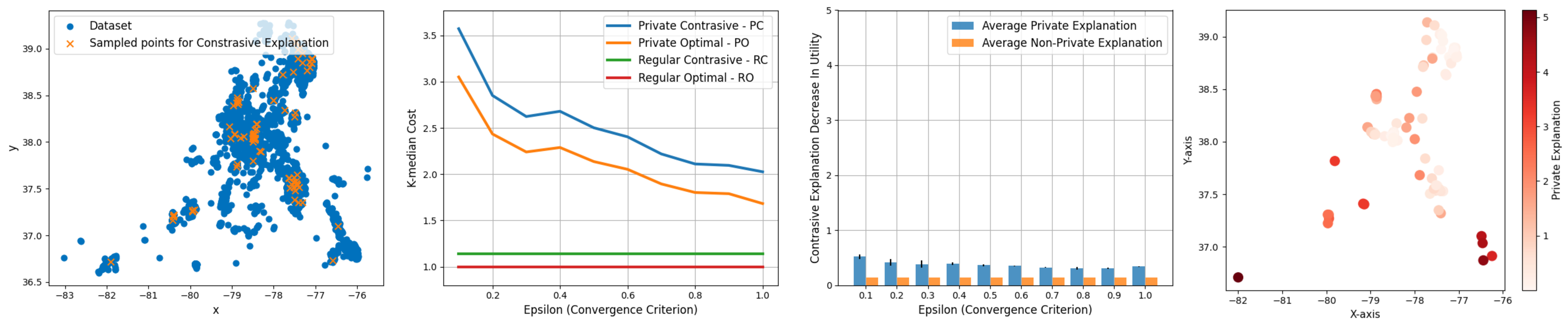
Experimental results. In this section, we focus solely on the Albemarle County dataset, with additional analyses and datasets presented in the Appendix. Figure 1(a) displays the dataset, highlighting the original data points with blue dots and the sampled points used for contrastive explanations with orange ’X’ markers. In Figure 1(b), we observe significant trends in the k-median clustering results for both private and non-private settings. Both the Private Optimal (PO) and Private Contrastive (PC) exhibit a downward trend in the private setting, indicating that as the $\epsilon$ budget increases, the error cost decreases, which underscores the trade-off between privacy and accuracy. The trends for non-private settings are depicted as straight lines, reflecting their independence from the privacy budget and are included for comparative purposes.

Our analysis shows a consistent gap between the Private Optimal (PO) and Private Contrastive (PC) across different levels of $\epsilon$ , marking a stable contrastive error that does not fluctuate with changes in the privacy budget. This stability is pivotal as it supports our goal of providing dependable explanations to agents, regardless of the $\epsilon$ value, ensuring that our approach adeptly balances privacy considerations with the demand for meaningful explainability.

The distinction between PO and PC arises because PO is derived from implementing the optimal k-median/k-means algorithm, while PC results from enforcing a centroid’s placement at a specific agent’s location, inherently producing a less optimal outcome due to this constraint. Initially, agents are presented with the optimal outcome (PO). When an agent inquires why a centroid is not positioned at their specific location, we offer a contrastive explanation (PC), which is naturally less optimal than the original result as it evaluates the utility change from hypothetically placing a centroid at that specific location. In this scenario, a higher score signifies lower utility, emphasizing the balance between providing personalized explanations and adhering to privacy constraints.

Figure 1(c) displays the average private explanation (APE) and average explanation (AE) with variance across different explanations. The average values of APE across multiple runs are relatively stable, irrespective of the privacy budget, reinforcing the robustness of our methodology against the constraints imposed by differential privacy.

Lastly, the heatmap in Figure 1(d) provides insights into how the relative spatial positioning affects the contrastive explanation. It vividly shows that the greater the distance a fixed centroid is from the distribution center, the larger the contrastive error, further illustrating the intricate dynamics of our clustering approach.

6 Discussion

Our work explores the design of private explanations for clustering, particularly focusing on the k-median and k-means objectives for Euclidean datasets. We formalize this as the PrivEC problem, which gives a contrastive explanation to each agent equal to the increase in utility when a cluster centroid is strategically positioned near them. The accuracy bounds of our algorithm match private clustering methods, even as they offer explanations for every user, within a defined privacy budget.
The related work in this domain has seen the development of algorithms for contrastive explanations, but our contribution stands out by integrating differential privacy guarantees. Our experiments demonstrate the resilience of our approach. Despite the added layer of providing differential private explanations on top of differential private clustering, the quality of our explanations remains uncompromised.

References

Balcan et al. [2017] Maria-Florina Balcan, Travis Dick, Yingyu Liang, Wenlong Mou, and Hongyang Zhang. Differentially private clustering in high-dimensional euclidean spaces. In Doina Precup and Yee Whye Teh, editors, Proceedings of the 34th International Conference on Machine Learning, ICML 2017, Sydney, NSW, Australia, 6-11 August 2017, volume 70 of Proceedings of Machine Learning Research, pages 322–331. PMLR, 2017. URL http://proceedings.mlr.press/v70/balcan17a.html.
Barrett et al. [2009] Christopher L Barrett, Richard J Beckman, Maleq Khan, VS Anil Kumar, Madhav V Marathe, Paula E Stretz, Tridib Dutta, and Bryan Lewis. Generation and analysis of large synthetic social contact networks. In Proceedings of the 2009 Winter Simulation Conference (WSC), pages 1003–1014. IEEE, 2009.
Bertsimas et al. [2022] Dimitris Bertsimas, Vassilis Digalakis Jr, Alexander Jacquillat, Michael Lingzhi Li, and Alessandro Previero. Where to locate covid-19 mass vaccination facilities? Naval Research Logistics (NRL), 69(2):179–200, 2022.
Boggess et al. [2023] Kayla Boggess, Sarit Kraus, and Lu Feng. Explainable multi-agent reinforcement learning for temporal queries. In Proceedings of the Thirty-Second International Joint Conference on Artificial Intelligence (IJCAI), 2023.
Charikar et al. [1999] Moses Charikar, Sudipto Guha, Éva Tardos, and David B Shmoys. A constant-factor approximation algorithm for the k-median problem. In Proceedings of the thirty-first annual ACM symposium on Theory of computing, pages 1–10, 1999.
Chen et al. [2021] Jiangzhuo Chen, Stefan Hoops, Achla Marathe, Henning Mortveit, Bryan Lewis, Srinivasan Venkatramanan, Arash Haddadan, Parantapa Bhattacharya, Abhijin Adiga, Anil Vullikanti, Aravind Srinivasan, Mandy L Wilson, Gal Ehrlich, Maier Fenster, Stephen Eubank, Christopher Barrett, and Madhav Marathe. Prioritizing allocation of covid-19 vaccines based on social contacts increases vaccination effectiveness. medRxiv, 2021.
Dasgupta and Gupta [2003] Sanjoy Dasgupta and Anupam Gupta. An elementary proof of a theorem of johnson and lindenstrauss. Random Structures & Algorithms, 22(1):60–65, 2003.
Dwork and Roth [2014] Cynthia Dwork and Aaron Roth. The algorithmic foundations of differential privacy. Found. Trends Theor. Comput. Sci., 9(3–4):211–407, aug 2014. ISSN 1551-305X. doi: 10.1561/0400000042. URL https://doi.org/10.1561/0400000042.
Feldman et al. [2017] Dan Feldman, Chongyuan Xiang, Ruihao Zhu, and Daniela Rus. Coresets for differentially private k-means clustering and applications to privacy in mobile sensor networks. In Proceedings of the 16th ACM/IEEE International Conference on Information Processing in Sensor Networks, pages 3–15, 2017.
Finkelstein et al. [2022] Mira Finkelstein, Lucy Liu, Yoav Kolumbus, David C Parkes, Jeffrey S Rosenschein, Sarah Keren, et al. Explainable reinforcement learning via model transforms. Advances in Neural Information Processing Systems, 35:34039–34051, 2022.
Georgara et al. [2022] Athina Georgara, Juan Antonio Rodríguez-Aguilar, and Carles Sierra. Privacy-aware explanations for team formation. In International Conference on Principles and Practice of Multi-Agent Systems, pages 543–552. Springer, 2022.
Ghazi et al. [2020] Badih Ghazi, Ravi Kumar, and Pasin Manurangsi. Differentially private clustering: Tight approximation ratios. In Proceedings of the 34th International Conference on Neural Information Processing Systems, NIPS’20, Red Hook, NY, USA, 2020. Curran Associates Inc. ISBN 9781713829546.
Goethals et al. [2022] Sofie Goethals, Kenneth Sörensen, and David Martens. The privacy issue of counterfactual explanations: explanation linkage attacks. arXiv preprint arXiv:2210.12051, 2022.
Gupta et al. [2010] Anupam Gupta, Katrina Ligett, Frank McSherry, Aaron Roth, and Kunal Talwar. Differentially private combinatorial optimization. In Proceedings of the Twenty-First Annual ACM-SIAM Symposium on Discrete Algorithms, SODA 2010, Austin, Texas, USA, January 17-19, 2010, pages 1106–1125. SIAM, 2010. doi: 10.1137/1.9781611973075.90. URL https://doi.org/10.1137/1.9781611973075.90.
Huang and Liu [2018] Zhiyi Huang and Jinyan Liu. Optimal differentially private algorithms for k-means clustering. In Proceedings of the 37th ACM SIGMOD-SIGACT-SIGAI Symposium on Principles of Database Systems, pages 395–408, 2018.
Johnson and Lindenstrauss [1984] William B Johnson and Joram Lindenstrauss. Extensions of lipschitz mappings into a hilbert space. In Conference on Modern Analysis and Probability, volume 26, pages 189–206. American Mathematical Society, 1984.
Kanungo et al. [2002] Tapas Kanungo, David M Mount, Nathan S Netanyahu, Christine D Piatko, Ruth Silverman, and Angela Y Wu. A local search approximation algorithm for k-means clustering. In Proceedings of the eighteenth annual symposium on Computational geometry, pages 10–18, 2002.
Kearns et al. [2014] Michael Kearns, Mallesh Pai, Aaron Roth, and Jonathan Ullman. Mechanism design in large games: Incentives and privacy. In Proceedings of the 5th conference on Innovations in theoretical computer science, pages 403–410, 2014.
Madumal et al. [2020] Prashan Madumal, Tim Miller, Liz Sonenberg, and Frank Vetere. Explainable reinforcement learning through a causal lens. In Proceedings of the AAAI conference on artificial intelligence, volume 34, pages 2493–2500, 2020.
Makarychev et al. [2019] Konstantin Makarychev, Yury Makarychev, and Ilya Razenshteyn. Performance of johnson-lindenstrauss transform for k-means and k-medians clustering. In Proceedings of the 51st Annual ACM SIGACT Symposium on Theory of Computing, pages 1027–1038, 2019.
Matoušek [2000] Jiří Matoušek. On approximate geometric k-clustering. Discrete & Computational Geometry, 24(1):61–84, 2000.
Mehrab et al. [2022] Zakaria Mehrab, Mandy L Wilson, Serina Chang, Galen Harrison, Bryan Lewis, Alex Telionis, Justin Crow, Dennis Kim, Scott Spillmann, Kate Peters, et al. Data-driven real-time strategic placement of mobile vaccine distribution sites. In Proceedings of the AAAI Conference on Artificial Intelligence, volume 36, pages 12573–12579, 2022.
Miller [2019] Tim Miller. Explanation in artificial intelligence: Insights from the social sciences. Artificial intelligence, 267:1–38, 2019.
Nguyen et al. [2023] Truc Nguyen, Phung Lai, Hai Phan, and My T Thai. Xrand: Differentially private defense against explanation-guided attacks. In Proceedings of the AAAI Conference on Artificial Intelligence, volume 37, pages 11873–11881, 2023.
Nissim and Stemmer [2018] Kobbi Nissim and Uri Stemmer. Clustering algorithms for the centralized and local models. In Algorithmic Learning Theory, pages 619–653. PMLR, 2018.
Patel et al. [2022] Neel Patel, Reza Shokri, and Yair Zick. Model explanations with differential privacy. In Proceedings of the 2022 ACM Conference on Fairness, Accountability, and Transparency, pages 1895–1904, 2022.
Rader et al. [2022] Benjamin Rader, Christina M Astley, Kara Sewalk, Paul L Delamater, Kathryn Cordiano, Laura Wronski, Jessica Malaty Rivera, Kai Hallberg, Megan F Pera, Jonathan Cantor, et al. Spatial modeling of vaccine deserts as barriers to controlling sars-cov-2. Communications Medicine, 2(1):141, 2022.
Reddy [2018] Chandan K Reddy. Data clustering: algorithms and applications. Chapman and Hall/CRC, 2018.
Saifullah et al. [2022] Saifullah Saifullah, Dominique Mercier, Adriano Lucieri, Andreas Dengel, and Sheraz Ahmed. Privacy meets explainability: A comprehensive impact benchmark. arXiv preprint arXiv:2211.04110, 2022.
Sreedharan et al. [2020] Sarath Sreedharan, Utkarsh Soni, Mudit Verma, Siddharth Srivastava, and Subbarao Kambhampati. Bridging the gap: Providing post-hoc symbolic explanations for sequential decision-making problems with inscrutable representations. arXiv preprint arXiv:2002.01080, 2020.
Sreedharan et al. [2021] Sarath Sreedharan, Siddharth Srivastava, and Subbarao Kambhampati. Using state abstractions to compute personalized contrastive explanations for ai agent behavior. Artificial Intelligence, 301:103570, 2021.
Stemmer [2020] Uri Stemmer. Locally private k-means clustering. In Shuchi Chawla, editor, Proceedings of the 2020 ACM-SIAM Symposium on Discrete Algorithms, SODA 2020, Salt Lake City, UT, USA, January 5-8, 2020, pages 548–559. SIAM, 2020. doi: 10.1137/1.9781611975994.33. URL https://doi.org/10.1137/1.9781611975994.33.
Stemmer and Kaplan [2018] Uri Stemmer and Haim Kaplan. Differentially private k-means with constant multiplicative error. Advances in Neural Information Processing Systems, 31, 2018.

Appendix A Related work: additional details

Our work considers differential privacy for explainable AI in general (XAI) and Multi-agent explanations (XMASE) in particular, focusing on post-hoc contrastive explanations for clustering.

Extensive experiments presented in Saifullah et al. [2022] demonstrate non-negligible changes in explanations of black-box ML models through the introduction of privacy. The findings in Patel et al. [2022] corroborate these observations regarding explanations for black-box feature-based models. These explanations involve creating local approximations of the model’s behavior around specific points of interest, potentially utilizing sensitive data. In order to safeguard the privacy of the data used during the local approximation process of an eXplainable Artificial Intelligence (XAI) module, the researchers have devised an innovative adaptive differentially private algorithm. This algorithm is designed to determine the minimum privacy budget required to generate accurate explanations effectively. The study undertakes a comprehensive evaluation, employing both empirical and analytical methods, to assess how the introduction of randomness inherent in differential privacy algorithms impacts the faithfulness of the model explanations.

Nguyen et al. [2023] considers feature-based explanations (e.g., SHAP) that can expose the top important features that a black-box model focuses on. To prevent such expose they introduced a new concept of achieving local differential privacy (LDP) in the explanations, and from that, they established a defense, called XRAND, against such attacks. They showed that their mechanism restricts the information that the adversary can learn about the top important features while maintaining the faithfulness of the explanations.

The analysis presented in Goethals et al. [2022] considers security concerning contrastive explanations. The authors introduced the concept of the ”explanation linkage attack”, a potential vulnerability that arises when employing instance-based strategies to derive contrastive explanations. To address this concern, they put forth the notion of k-anonymous contrastive explanations. Furthermore, the study highlights the intricate balance between transparency, fairness, and privacy when incorporating k-anonymous explanations. As the degree of privacy constraints is heightened, a discernible trade-off comes into play: the quality of explanations and, consequently, transparency are compromised.

Amongst the three types of eXplainable AI mentioned earlier, the maintenance of privacy during explanation generation incurs a certain cost. This cost remains even if an expense was previously borne during the creation of the original model. However, in our proposed methodology for generating contrastive explanations in clustering scenarios, once the cost of upholding differential privacy in the initial solution is paid, no additional expenses are requisite to ensure differential privacy during the explanation generation phase.

Closer to our application is the study that investigates the privacy aspects concerning contrastive explanations in the context of team formation Georgara et al. [2022]. In this study, the authors present a comprehensive framework that integrates team formation solutions with their corresponding explanations, while also addressing potential privacy concerns associated with these explanations. To accomplish this, the authors introduce a privacy breach detector (PBD) that is designed to evaluate whether the provision of an explanation might lead to privacy breaches. The PBD consists of two main components: (a) A belief updater (BU), calculates the posterior beliefs that a user is likely to form after receiving the explanation. (b) A privacy checker (PC), examines whether the user’s expected posterior beliefs surpass a specified belief threshold, indicating a potential privacy breach. However, the research is still in its preliminary stages and needs a detailed evaluation of the privacy breach detector.

Our contribution includes the development of comprehensive algorithms for generating contrastive explanations with differential privacy guarantees. We have successfully demonstrated the effectiveness of these algorithms by providing rigorous proof for their privacy guarantees and conducting extensive experiments that showcased their accuracy and utility. In particular, we have shown the validity of our private explanations for clustering based on the $k$ -median and $k$ -means objectives for Euclidean datasets. Moreover, our algorithms have been proven to have the same accuracy bounds as the best private clustering methods, even though they provide explanations for all users, within a bounded privacy budget. Notably, our experiments in the dedicated experiments section reveal that the epsilon budget has minimal impact on the explainability of our results, further highlighting the robustness of our approach.

There has been a lot of work on private clustering and facility location, starting with Gupta et al. [2010], which was followed by a lot of work on other clustering problems in different privacy models, e.g., Huang and Liu [2018], Stemmer [2020], Stemmer and Kaplan [2018], Nissim and Stemmer [2018], Feldman et al. [2017]. Gupta et al. [2010] demonstrated that the additive error bound for points in a metric space involves an $O(\Delta k^{2}\log{n}/\epsilon)$ term, where $\Delta$ is the space’s diameter. Consequently, all subsequent work, including ours, assumes points are restricted to a unit ball.

Appendix B Additional proofs for PECluster

Theorem 5.

(Full version of Theorem 1) The solution $c$ and $\text{cost}{(S_{\epsilon})}$ released by Algorithm 3 are $\epsilon$ -DP. For all clients $i$ , the value $\text{cost}(S_{\epsilon})-\text{cost}{S^{(i)}_{\epsilon}}$ released by Algorithm 4 is $\epsilon$ - $x_{i}$ -exclusive DP.

Proof.

It follows that $\text{cost}(S_{\epsilon})$ is the direct results (using no private information) of $Y$ , which is $\epsilon/2$ -differentially private coreset. By the post-processing property, $\text{cost}(S_{\epsilon})$ is $\epsilon/2$ -DP (which implies $\epsilon$ -DP).

$c$ is the output of DimReverse that is $\epsilon/2$ -DP w.r.t. the input $(X_{1},X_{2},\ldots,X_{k})$ . By composition, $c$ is $\epsilon$ -DP since the input $(X_{1},X_{2},\ldots,X_{k})$ is calculated partially from $Y$ , which is $\epsilon/2$ -DP.

For each explanations $S^{(i)}_{\epsilon}$ , let $D,D^{\prime}:D\setminus\{x_{i}\}\sim D^{\prime}\setminus\{x_{i}\}$ , let $S^{(i)}_{\epsilon}(Y^{D},x_{i})$ be the value of $S^{(i)}_{\epsilon}$ with input dataset $D$ (and $Y^{D}$ as the private coreset of $D$ respectively) and a fixed center $x_{i}$ , let $T=\{Y:S^{(i)}_{\epsilon}(Y,x_{i})\in S\}$ , we have $D\sim D^{\prime}$ and therefore:

$\displaystyle\Pr[S^{(i)}_{\epsilon}(D,x_{i})\in S]$	$\displaystyle=\Pr[Y^{D}\in T]$	(15)
	$\displaystyle\leq e^{\epsilon/2}\Pr[Y^{D^{\prime}}\in T]$	(16)
	$\displaystyle=e^{\epsilon/2}\Pr[S^{(i)}_{\epsilon}(D^{\prime},x_{i})\in T],$	(17)

which implies that $\text{cost}(S^{(i)}_{\epsilon})-\text{cost}(S_{\epsilon})$ is $\epsilon$ - $x_{i}$ -exclusive DP, since $\text{cost}(S_{\epsilon})$ is $\epsilon/2$ -DP (which implies $\epsilon/2$ - $x_{i}$ -exclusive DP). ∎

Lemma 7.

(Full version of Lemma 1) With probability at least $1-\beta$ , $(c_{1},\ldots,c_{k})$ is a $(w,t)$ -approximation of $OPT$ , where:

	$\displaystyle w$	$\displaystyle=w^{\prime\prime}(1+\alpha),$		(18)
	$\displaystyle t$	$\displaystyle=\mathcal{O}_{p,\alpha,w^{\prime\prime}}\left(\frac{(k/\beta)^{O_{p,\alpha}(1)}}{\epsilon}.\text{polylog}(n/\beta)\right)$		(19)

Proof.

This result derives from Theorem 48 of Ghazi et al. [2020] (From Eq(20) to Eq(24) of Ghazi et al. [2020]). ∎

Lemma 8.

(Full version of Lemma 2) Fix an $i$ . If $OPT_{i}\geq w^{\prime\prime}(1+\alpha)OPT+t^{(i)}$ , then with probability at least $1-2\beta$ , cost( $S_{\epsilon}$ ) and cost( $S^{(i)}_{\epsilon}$ ) released by Algorithm 3 and 4 satisfies that $cost(S^{(i)}_{\epsilon})>cost(S_{\epsilon}$ )

Proof.

By the result of Lemma 9, with probability $1-2\beta$ we have:

$\displaystyle cost(S^{(i)}_{\epsilon})$	$\displaystyle\geq OPT_{i}$	(20)
	$\displaystyle\geq w^{\prime\prime}(1+\alpha)OPT+t^{(i)}$	(21)
	$\displaystyle\geq w^{\prime\prime}(1+\alpha)\frac{cost(S_{\epsilon})-\Omega_{p,\alpha,w^{\prime\prime}}\left(\frac{(k/\beta)^{O_{p,\alpha}(1)}}{\epsilon}.\text{polylog}(n/\beta)\right)}{w^{\prime\prime}(1+\alpha)}+t^{(i)}$	(22)
	$\displaystyle=cost(S_{\epsilon})+t^{(i)}-\Omega_{p,\alpha,w^{\prime\prime}}\left(\frac{(k/\beta)^{O_{p,\alpha}(1)}}{\epsilon}.\text{polylog}(n/\beta)\right).$	(23)

Lemma 9.

(Johnson-Lindenstrauss (JL) Lemma Johnson and Lindenstrauss [1984], Dasgupta and Gupta [2003]) Let $v$ be any $d$ -dimensional vector. Let $\mathcal{S}$ denote a random $d^{\prime}$ -dimensional subspace of $\mathbb{R}^{d}$ and let $\Pi_{S}$ denote the projection from $\mathbb{R}^{d}$ to $\mathcal{S}$ . Then, for any $\zeta\in(0,1)$ we have

\displaystyle\Pr\left[\|v\|_{2}\approx_{1+\zeta}\sqrt{d/d^{\prime}}\|\Pi_{\mathcal{S}}(v)\|_{2}\right]\geq 1-2\exp\left(-\frac{d^{\prime}\zeta^{2}}{100}\right)

(24)

Lemma 10.

(Dimensionality Reduction for $(k,p)$ -Cluster Makarychev et al. [2019]) For every $\beta>0,\tilde{\alpha}<1,p\geq 1,k\in\mathbb{N}$ , there exists $d^{\prime}=O_{\tilde{\alpha}}(p^{4}\log(k/\beta))$ . Let $\mathcal{S}$ be a random d-dimensional subspace of $\mathbb{R}^{d}$ and $\Pi_{\mathcal{S}}$ denote the projection from $\mathbb{R}^{d}$ to $\mathcal{S}$ . With probability $1-\beta$ , the following holds for every partition $\mathcal{X}=(X_{1},\ldots,X_{k})$ of $X$ :

\displaystyle cost^{p}(\mathcal{X})\approx_{1+\tilde{\alpha}}(d/d^{\prime})^{p/2}cost^{p}(\Pi_{\mathcal{S}}(\mathcal{X})),

(25)

where $\Pi_{\mathcal{S}}(\mathcal{X})$ denotes the partition $(\Pi_{\mathcal{S}}(X_{1}),\ldots,\Pi_{\mathcal{S}}(X_{k}))$ .

Theorem 6.

(Full version of Theorem 2) Fix an $i$ . With probability at least $1-\beta$ , cost( $S^{(i)}_{\epsilon}$ ) released by Algorithm 4 is a $(w,t)$ -approximation of the optimal cost $OPT_{i}$ , in which:

	$\displaystyle w$	$\displaystyle=w^{\prime}(1+\alpha)$
	$\displaystyle t$	$\displaystyle=w^{\prime}\mathcal{O}_{k,p}\left(\frac{2^{O_{p,\alpha}(d)}k^{2}\log^{2}{n}}{\epsilon}.\text{polylog}(\frac{n}{\beta}\right),$

and $OPT_{i}$ is the optimal $(k,p)$ -clustering cost with a center is fixed at position $x_{i}$ .

Proof.

Let $\tilde{\mathbf{X}}=(\tilde{x}_{1},\tilde{x}_{2},\ldots,\tilde{x}_{n})$ and $X=(x^{\prime}_{1},x^{\prime}_{2},\ldots,x^{\prime}_{n})$ , setting $\alpha^{\prime}=0.1\alpha$ , applying Lemma 10, we have:

\displaystyle{OPT}_{i}^{\tilde{d}}\leq\left(\frac{d^{\prime}}{d}\right)^{p/2}(1+0.1\alpha)OPT_{i}^{d}.

(26)

By standard concentration, it can be proved that $\|x^{\prime}_{i}\|\leq 1/\Lambda$ with probability $0.1\beta/n$ as follows:

Using Lemma 9, we have:

\displaystyle\Pr\left[\|x\|>\frac{1}{1+\zeta}\sqrt{d/d^{\prime}}\|x^{\prime}\|\right]

\displaystyle\geq 1-2\exp(-d^{\prime}\zeta^{2}/100).

(27)

Since $x$ is in the unit ball, $\|x\|<1$ , which leads to:

\displaystyle\Pr\left[\|x^{\prime}\|<(1+\zeta)\sqrt{d^{\prime}/d}\right]

\displaystyle\geq 1-2\exp(-d^{\prime}\zeta^{2}/100).

(28)

Setting $\zeta=\sqrt{\frac{log(n/\beta)}{0.01}}-1$ , $\Lambda=\frac{1}{1+\zeta}\sqrt{d/d^{\prime}}=\sqrt{\frac{0.01}{\log{(n/\beta)}}.\frac{d}{d^{\prime}}}$ , we have:

$\displaystyle\Pr[\\|x^{\prime}\\|<1/\Lambda]$	$\displaystyle\geq 1-2\exp(-\frac{d^{\prime}\zeta^{2}}{100})$	(29)
	$\displaystyle>1-2\exp(-d^{\prime}\log(n/\beta))$	(30)
	$\displaystyle>1-2\beta/n,$	(31)

By union bound on all $i$ , then with probability at least $1-2\beta$ , $x^{\prime}_{i}=\Lambda\tilde{x}_{i}$ for all $i$ . Since $Y$ is the output of PrivateCoreset with input $X$ , then by Theorem 38 of Ghazi et al. [2020], $Y$ is a $(0.1\alpha,t)$ -coreset of $X^{\prime}$ (with probability at least $1-\beta$ ), with $t^{\prime}$ as:

\displaystyle t^{\prime}=O_{p,\alpha}\left(\frac{2^{O_{p,\alpha}(d^{\prime})}k^{2}\log^{2}{n}}{\epsilon}\log\left(\frac{n}{\beta}\right)+1\right)

(32)

Let $(y_{1},y_{2},\ldots,y_{k})$ be the solution of NonPrivateApproxFC in peCluster for a fixed $i$ , $(y^{*}_{1},y^{*}_{2},\ldots,y^{*}_{k})$ be the optimal solution of the clustering with fixed center at $x^{\prime}_{i}$ on $X$ , $OPT_{Y}$ be the optimal cost of the clustering with fixed center at $x^{\prime}_{i}$ on $Y$ . By the $w^{\prime}$ -approximation property of NonPrivateApproximationFC, we have:

$\displaystyle cost_{Y}(y_{1},y_{2},\ldots,y_{k})$	$\displaystyle\leq w^{\prime}OPT_{Y}$	(33)
	$\displaystyle\leq w^{\prime}cost_{Y}(y^{}_{1},y^{}_{2},\ldots,y^{*}_{k})$	(34)
	$\displaystyle\leq w^{\prime}(1+0.1\alpha)cost_{\mathbf{X}^{\prime}_{1..n}}(y^{}_{1},y^{}_{2},\ldots,y^{*}_{k})+w^{\prime}t^{\prime}$	(35)
	$\displaystyle=w^{\prime}(1+0.1\alpha)OPT^{d^{\prime}}_{i}+w^{\prime}t^{\prime}.$	(36)

Composing with Lemma 10, we have:

$\displaystyle cost_{Y}(y_{1},y_{2},\ldots,y_{k})$	$\displaystyle\leq w^{\prime}(1+0.1\alpha)OPT^{d^{\prime}}_{i}+w^{\prime}t^{\prime}$	(37)
	$\displaystyle\leq\Lambda^{p}w^{\prime}(1+0.1\alpha)OPT^{\tilde{d}}_{i}+w^{\prime}t^{\prime}$	(38)
	$\displaystyle\leq\Lambda^{p}w^{\prime}(1+0.1\alpha)(1+0.1\alpha)\left(\frac{d^{\prime}}{d}\right)^{p/2}OPT^{d}_{i}+w^{\prime}t^{\prime}$	(39)
	$\displaystyle\leq w^{\prime}(1+\alpha)OPT^{d}_{i}\left(\frac{0.01}{\log(n/\beta)}\right)^{p/2}+w^{\prime}t^{\prime},\mbox{ since $\Lambda^{2}d^{\prime}/d=\Theta(1/\log(n/\beta))$}$	(40)

Finally, since

$\displaystyle cost(S^{(i)}_{\epsilon})$	$\displaystyle=cost_{Y}(y_{1},y_{2},\ldots,y_{k})\left(\frac{\log(n/\beta)}{0.01}\right)^{p/2}$	(41)
	$\displaystyle\leq w^{\prime}(1+\alpha)OPT^{d}_{i}+\Theta(w^{\prime}t^{\prime}(\log(n/\beta)^{p/2})$	(42)
	$\displaystyle\overset{(a)}{\leq}w^{\prime}(1+\alpha)OPT^{d}_{i}+w^{\prime}\Theta\left(\frac{2^{O_{p,\alpha}(d^{\prime})}k^{2}\log^{2}{n}}{\epsilon}\log\left(\frac{n}{\beta}\right)(\log(n/\beta))^{p/2}\right)$	(43)
	$\displaystyle\overset{(b)}{\leq}w^{\prime}(1+\alpha)OPT^{d}_{i}+w^{\prime}\Theta\left(\frac{(k/\beta)^{O_{p,\alpha}(1)}k^{2}\log^{2}{n}}{\epsilon}\log\left(\frac{n}{\beta}\right)(\log(n/\beta))^{p/2}\right)$	(44)
	$\displaystyle\overset{(c)}{\leq}w^{\prime}(1+\alpha)OPT^{d}_{i}+w^{\prime}\Theta\left(\frac{(k/\beta)^{O_{p,\alpha}(1)}(k/\beta)^{2}\log^{2}(n/\beta)}{\epsilon}\log\left(\frac{n}{\beta}\right)(\log(n/\beta))^{p/2}\right)$	(45)
	$\displaystyle=w^{\prime}(1+\alpha)OPT^{d}_{i}+w^{\prime}\Theta\left(\frac{(k/\beta)^{O_{p,\alpha}(1)}}{\epsilon}.\text{polylog}(n/\beta)\right),$	(46)

where in $(a)$ we substitute the value of $t^{\prime}$ , and $(b)$ is because $d^{\prime}=O_{\alpha}(p^{4}\log(n/\beta))$ , and $(c)$ is because $\beta<1$ , and the Lemma follows. ∎

Set $t^{(i)}=\Omega_{p,\alpha,w^{\prime\prime}}\left(\frac{(k/\beta)^{O_{p,\alpha}(1)}}{\epsilon}.\text{polylog}(n/\beta)\right)$ and the Lemma follows. ∎

Appendix C Additional proofs for $k$ -median algorithm

Definition 9.

The solution of the $k$ -median problem (with demands and a center fixed at a location $C$ ) can be formulated as finding the optimal solution of the following Integer program (IP):

minimize	$\displaystyle\sum_{i,j\in N}d_{j}c_{ij}x_{ij}$	(48)
$\displaystyle\text{subject to }\sum_{i\in N}x_{ij}$	$\displaystyle=1\text{ for each $j\in N$}$	(49)
$\displaystyle x_{ij}$	$\displaystyle\leq y_{i}\text{ for each $i,j\in N$}$	(50)
$\displaystyle\sum_{j\in N}y_{i}$	$\displaystyle=k$	(51)
$\displaystyle x_{ij}$	$\displaystyle\in\{0,1\}\text{ for each $i,j\in N$}$	(52)
$\displaystyle y_{i}$	$\displaystyle\in\{0,1\}\text{ for each $i\in N$}$	(53)
$\displaystyle y_{C}$	$\displaystyle=1\text{ for a fixed $C\in N$}$	(54)
$\displaystyle x_{CC}$	$\displaystyle=1\text{ for a fixed $C\in N$}.$	(55)

Lemma 11.

Locations $i,j\in N^{\prime}$ satisfy: $c_{ij}>4\max(\bar{C}_{i},\bar{C}_{j})$ .

Proof.

The lemma follows the demands moving step (in the first step of the algorithm): for every $j$ to the right of $i$ (which means $\bar{C}_{j}\geq\bar{C}_{i}$ ) and within the distance of $\bar{C}_{j}$ (that also covers all points within distance $\bar{C}_{i}$ ), we move all demands of $j$ to $i$ , hence $j$ will not appear in $N^{\prime}$ . ∎

Lemma 12.

(Lemma 4 of Charikar et al. [1999]) For any feasible integer solution $(x^{\prime},y^{\prime})$ for the input with modified demands, there is a feasible integer solution for the original input with cost at most $4\bar{C}_{LP}$ plus the cost of $(x^{\prime},y^{\prime})$ with demands $d^{\prime}$ .

Lemma 13.

(Theorem 6 of Charikar et al. [1999]) There is a $1/2$ -restricted solution $(x^{\prime},y^{\prime})$ of cost at most $2\bar{C}_{LP}$ .

Appendix D Additional proofs for $k$ -means algorithm

Lemma 14.

(Lemma 2.1 of Kanungo et al. [2002]) Given a finite subset $S$ of points in $\mathbb{R}^{d}$ , let $c$ be the centroid of $S$ . Then for any $c^{\prime}\in\mathbb{R}^{d}$ , $\Delta(S,c^{\prime})=\Delta(S,c)+|S|\Delta(c,c^{\prime})$ .

Lemma 15.

(Full version of Lemma 5) Let $S$ be $1$ -stable set and $O$ be the optimal set of $k$ centers, we have $\Delta(O)-3\Delta(S)+2R\geq 0$ , where $R=\sum_{q\in P}\Delta(q,s_{o_{q}})$ .

Proof.

Since $S$ is $1$ -stable, we have for each swap pair:

	$\displaystyle\sum_{q\in N_{O}(o)}$	$\displaystyle\big{(}\Delta(q,o)-\Delta(q,s_{q})\big{)}$		(56)
	$\displaystyle+\sum_{q\in N_{S}(s)\setminus N_{O}(o)}$	$\displaystyle\big{(}\Delta(q,s_{o_{q}})-\Delta(q,s)\big{)}\geq 0.$		(57)

We will sum up the inequality above for all swap pairs. For the left term, the sum is overall $o\in O$ :

		$\displaystyle\sum_{o\in O}\sum_{q\in N_{O}(o)}\big{(}\Delta(q,o)-\Delta(q,s_{q})\big{)}$		(58)
	$\displaystyle=$	$\displaystyle\sum_{q\in P}\big{(}\Delta(q,o)-\Delta(q,s_{q})\big{)},$		(59)

Since each $o\in O$ will appear exactly once, and $\cup_{o\in O}q\in N_{O}(o)$ will cover all points in $P$ .

For the right term, the sum is over all $s$ that is being swapped out. We note that each $s$ can be swapped out at most twice, hence:

	$\displaystyle\sum_{s\text{ being swapped out}}\sum_{q\in N_{S}(s)}$	$\displaystyle\big{(}\Delta(q,s_{o_{q}})-\Delta(q,s)\big{)}$		(60)
	$\displaystyle\leq 2\sum_{q\in P}$	$\displaystyle\big{(}\Delta(q,s_{o_{q}})-\Delta(q,s)\big{)}$		(61)

When we combine the two terms, we have:

$\displaystyle\sum_{q\in P}\big{(}\Delta(q,o)-\Delta(q,s_{q})\big{)}+2\sum_{q\in P}\big{(}\Delta(q,s_{o_{q}})-\Delta(q,s)\big{)}$	$\displaystyle\geq 0$	(62)
$\displaystyle\sum_{q\in P}\Delta(q,o_{q})-3\sum_{q\in P}\Delta(s,s_{q})+2\sum_{q\in P}\Delta(q,s_{o_{q}})$	$\displaystyle\geq 0$	(63)
$\displaystyle\Delta(O)-3\Delta(S)+2R$	$\displaystyle\geq 0,$	(64)

and the Lemma follows. ∎

Lemma 16.

(Proof in Lemma 2.2 & 2.3 of Kanungo et al. [2002]) Let $\alpha^{2}=\frac{\Delta(S)}{\Delta(O)}$ , we have $\sum_{q\in P}dist(q,o_{q})dist(q,s_{q})\leq\frac{\Delta(S)}{\alpha}$

Lemma 17.

(Full version of Lemma 6) With $R$ and $\alpha$ defined as above: $R\leq 2\Delta(O)+(1+2/\alpha)\Delta(S)$ .

Proof.

By Lemma 15, we have:

$\displaystyle R$	$\displaystyle=\sum_{q\in P}\Delta(q,s_{o_{q}})$	(65)
	$\displaystyle=\sum_{o\in O}\sum_{q\in N_{O}(o)}\Delta(q,s_{o})$	(66)
	$\displaystyle=\sum_{o\in O\setminus\sigma}\sum_{q\in N_{O}(o)}\Delta(q,s_{o})+\sum_{q\in N_{O}(\sigma)}\Delta(q,\sigma)$	(67)
	$\displaystyle=\sum_{o\in O\setminus\sigma}\Delta(N_{O}(o),s_{o})+\Delta(N_{O}(\sigma),\sigma)$	(68)
	$\displaystyle\overset{(a)}{=}\sum_{o\in O\setminus\sigma}\big{(}\Delta(N_{O}(o),o)+\|N_{O}(o)\|\Delta(o,s_{o})\big{)}+\Delta(N_{O}(\sigma),\sigma)$	(69)
	$\displaystyle=\sum_{o\in O\setminus\sigma}\sum_{q\in N_{O}(o)}\big{(}\Delta(q,o)+\Delta(o,s_{o})\big{)}+\sum_{q\in N_{O}(\sigma)}\Delta(q,\sigma)+\Delta(\sigma,o_{\sigma})$	(70)
	$\displaystyle=\sum_{o\in O}\sum_{q\in N_{O}(o)}\big{(}\Delta(q,o)+\Delta(o,s_{o})\big{)}$	(71)
	$\displaystyle\overset{(b)}{=}\sum_{o\in O}\sum_{q\in N_{O}(o)}\big{(}\Delta(q,o)+\Delta(o,s_{q})\big{)}$	(72)
	$\displaystyle\leq\sum_{q\in P}\big{(}\Delta(q,o_{q})+\Delta(o_{q},s_{q})\big{)}$	(73)
	$\displaystyle\overset{(c)}{\leq}\Delta(O)+\sum_{q\in P}(dist(o_{q},q)+dist(q,s_{q}))^{2}$	(74)
	$\displaystyle=2\Delta(O)+\Delta(S)+2\sum_{q\in P}dist(q,o_{q})dist(q,s_{q})$	(75)
	$\displaystyle\overset{(d)}{\leq}2\Delta(O)+\Delta(S)+(2/\alpha)\Delta(S),$	(76)

where $(a)$ is because Lemma 14 applies for all $o\in O\setminus\sigma$ , $(b)$ is because $\Delta(o,s_{o})\leq\Delta(o,s_{q})$ , $(c)$ is because the triangle inequality applies for $\Delta(o_{q},s_{q})$ and $(d)$ is because of Lemma 16 and the Lemma follows. ∎

D.1 Swap pairs mapping

In this section, we describe the swap pairs mapping scheme for the $k$ -means with a fixed center algorithm. We adapt the scheme of Matoušek [2000] to accommodate the fixed center. We discuss the modifications in Section 4.2. Here we discuss the complete mapping scheme.

At the last iteration of the algorithm, we always have a candidate set of centers $S$ that is $1$ -stable, i.e., no single feasible swap can decrease its cost. We then analyze some hypothetical swapping schemes, in which we try to swap a center $s\in S$ with an optimal center $o\in O$ . We utilize the fact that such single swaps do not decrease the cost to create some relationships between $\Delta(S)$ and $\Delta(O)$ –the optimal cost. Particularly, these relationships are stated in Lemma 15 and Lemma 17.

Let $\sigma$ be the fixed center. We note that $\sigma\in S$ and $\sigma\in O$ . Let $s_{o}$ be the closest center in $S$ for an optimal center $o\in O$ , which means $o$ is captured by $s_{o}$ . It follows that $s_{\sigma}=\sigma$ . A center $s\in S$ may capture no optimal center (we call it lonely). We partition both $S$ and $O$ into $S_{1},\ldots,S_{r}$ and $O_{1},\ldots,O_{r}$ that $|S_{i}|=|O_{i}|$ for all $i$ .

We construct each pair of partitions $S_{i},O_{i}$ as follows: let $s$ be a non-lonely center, $O_{i}=\{o\in O:s_{o}=s\}$ , i.e., $O_{i}$ is the set of all optimal centers that are captured by $s$ . Now, we compose $s$ with $|O_{i}|-1$ lonely centers (which are not partitioned into any group from $S$ ) to form $S_{i}$ . It is clear that $|S_{i}|=|O_{i}|\geq 1$ .

We then generate swap pairs for each pair of partitions $S_{i},O_{i}$ by the following cases:

•

$|S_{i}|=|O_{i}|=1$ : let $S_{i}=\{s\},O_{i}=\{o\}$ , generate a swap pair $\{s,o\}$ .
•

$|S_{i}|=|O_{i}|=m>1$ : let $S_{i}=\{s,s_{1..m-1}\}$ in which $s_{1..m-1}$ are $m-1$ lonely centers, let $O_{i}=\{o_{1..m}\}$ , generate $m-1$ swap pairs $\{s_{j},o_{j}\}$ for $j=1..m-1$ . Also, we generate a swap pair of $\{s_{1},o_{m}\}$ . Please note that $s$ does not belong to any swap pair, each $o_{j}$ belongs to exactly one swap pair, and each $s_{j}$ belongs to at most two swap pairs.

We then guarantee the following $3$ properties of our swap pairs:

1.

each $o\in O$ is swapped in exactly once
2.

each $s\in S$ is swapped out at most twice
3.

for each swap pair $\{s,o\}$ , $s$ either captures only $o$ , or $s$ is lonely (captures nothing).

D.2 $\gamma$ -approximate candidate center set for fixed-center $k$ -means.

We describe how to generate a $\gamma$ -approximate candidate center set for $k$ -means with fixed center $\sigma$ for a dataset $X\subset\mathbb{R}^{d}$ . From the result of Matoušek [2000], we create a set $C^{\prime}$ which is a $\gamma$ -approximation centroid set of $X$ . We will prove that $C=C^{\prime}\cup\{\sigma\}$ forms a $\gamma$ -approximate candidate center set for $k$ -means with fixed center $\sigma$ .

Definition 10.

Let $S\subset\mathbb{R}^{d}$ be a finite set with its centroid $c(S)$ . A $\gamma$ -tolerance ball of $S$ is the ball centered at $c(S)$ and has radius of $\frac{\gamma}{3}\rho(S)$ .

Definition 11.

Let $X\subset\mathbb{R}^{d}$ be a finite set. A finite set $C^{\prime}\in\mathbb{R}^{d}$ is a $\gamma$ -approximation centroid set of $X$ if $C^{\prime}$ intersects the $\gamma$ -tolerance ball of each nonempty $S\subseteq X$ .

Lemma 18.

(Theorem 4.4 of Matoušek [2000]) We can compute $C^{\prime}$ –a $\gamma$ -approximation centroid set of $X$ that has size of $O(n\gamma^{-d}\log(1/\gamma))$ in time $O(n\log{n}+n\gamma^{-d}\log(1/\gamma))$ .

Theorem 7.

Let $C=C^{\prime}\cup\{\sigma\}$ , in which $C^{\prime}$ is a $\gamma$ -approximation centroid set computed as Lemma 18, then $C$ is a $\gamma$ -approximate candidate center set for $k$ -means with fixed center $\sigma$ .

Proof.

Let $O=(O_{1},O_{2},\ldots,O_{k})$ be the optimal clustering in which $O_{1}$ is the cluster whose center is $\sigma$ (we denote it as $O_{\sigma}$ ). For any $S\subset\mathbb{R}^{d}$ , we define $cost_{S}(c)=\sum_{x\in S}\|x-c\|^{2}$ and $cost(S)=cost_{S}(c(S))$ in which $c(S)$ is the centroid of $S$ . By Definition 7, we will prove that there exists a set $c_{1},c_{2},\ldots,c_{k}\subset C$ and $c_{1}=\sigma$ such that $cost(c_{1},c_{2},\ldots,c_{k})\leq(1+\gamma)cost(O)$ . We adapt the analysis of Matoušek [2000] for the special center $\sigma$ –which is not a centroid as other centers in $k$ -means.

First, we analyze the optimal cost. For any cluster except $O_{\sigma}$ , its center is also the centroid $c(O_{i})$ of the cluster, while $O_{\sigma}$ must have center $\sigma$ :

	$\displaystyle cost(O)$	$\displaystyle=\sum_{x\in O_{\sigma}}\\|x-\sigma\\|^{2}+\sum_{i=2..k}\sum_{x\in O_{i}}\\|x-c(O_{i})\\|^{2}$		(77)
		$\displaystyle=cost_{O\sigma}(\sigma)+\sum_{i=2..k}cost(O_{i})$		(78)

Now, we construct $\{c_{1},\ldots,c_{k}\}$ as follows: setting $c_{1}=\sigma$ , for $i=2..k$ , $c_{i}\in C^{\prime}$ is the candidate center that intersects the $\gamma$ -tolerance ball of cluster $O_{i}$ . For $O_{\sigma}$ , $cost_{O_{\sigma}}(\sigma)=cost(O_{\sigma})$ . For other clusters, $cost_{O_{i}}(c_{i})\leq(1+\gamma)cost(O_{i})$ as below:

$\displaystyle cost_{O_{i}}(c_{i})$	$\displaystyle=\sum_{x\in O_{i}}\\|x-c_{i}\\|^{2}$	(79)
	$\displaystyle\leq\sum_{x\in O_{i}}(\\|x-c(O_{i})\\|+\\|c(O_{i})-c_{i}\\|)^{2}$	(80)
	$\displaystyle=cost(O_{i})+2\\|c_{i}-c(O_{i})\\|\sum_{x\in O_{i}}\\|x-c(O_{i})\\|+\|O_{i}\|\\|c_{i}-c(O_{i})\\|^{2}$	(81)
	$\displaystyle\leq cost(O_{i})+2\gamma/3\rho(O_{i})\sqrt{\|O_{i}\|}\sqrt{cost(O_{i})}+\|O_{i}\|(\gamma/3\rho(O_{i}))^{2}$	(82)
	$\displaystyle\leq cost(O_{i})+(2/3)\gamma cost(O_{i})+(\gamma^{2}/9)cost(O_{i})$	(83)
	$\displaystyle\leq(1+\gamma/3)^{2}cost(O_{i})$	(84)
	$\displaystyle\leq(1+\gamma)cost(O_{i}).$	(85)

Let $(S_{1},S_{2},\ldots,S_{k})$ be the Voronoi partition with centers $(c_{1},c_{2},\ldots,c_{k})$ , i.e., $S_{i}$ are points in the Voronoi region of $c_{i}$ in the Voronoi diagram created by $c_{1},\ldots,c_{k}$ , we have:

$\displaystyle cost(c_{1},c_{2},\ldots,c_{k})$	$\displaystyle=cost_{S_{1}}(\sigma)+\sum_{i=2..k}cost(S_{i})$	(86)
	$\displaystyle\overset{(a)}{\leq}cost_{S_{1}}(\sigma)+\sum_{i=2..k}cost_{S_{i}}(c_{i})$	(87)
	$\displaystyle\overset{(b)}{\leq}cost_{O_{\sigma}}(\sigma)+\sum_{i=2..k}cost_{O_{i}}(c_{i})$	(88)
	$\displaystyle\overset{(c)}{\leq}cost_{O_{\sigma}}(\sigma)+(1+\gamma)\sum_{i=2..k}cost(O_{i})$	(89)
	$\displaystyle\leq(1+\gamma)cost(O),$	(90)

where $(a)$ is because $cost(S_{i})$ implies its minimal cost for any center, $(b)$ is because $S_{i}$ s are picked by Voronoi partition which minimies the cost over $k$ partitions of seletecd $k$ centers, and $(c)$ is because $cost_{O_{i}}(c_{i})\leq(1+\gamma)cost(O_{i})$ as we proved above, and the Theorem follows. ∎

D.3 Additional details on experiments

D.3.1 Datasets and Experimental Setup

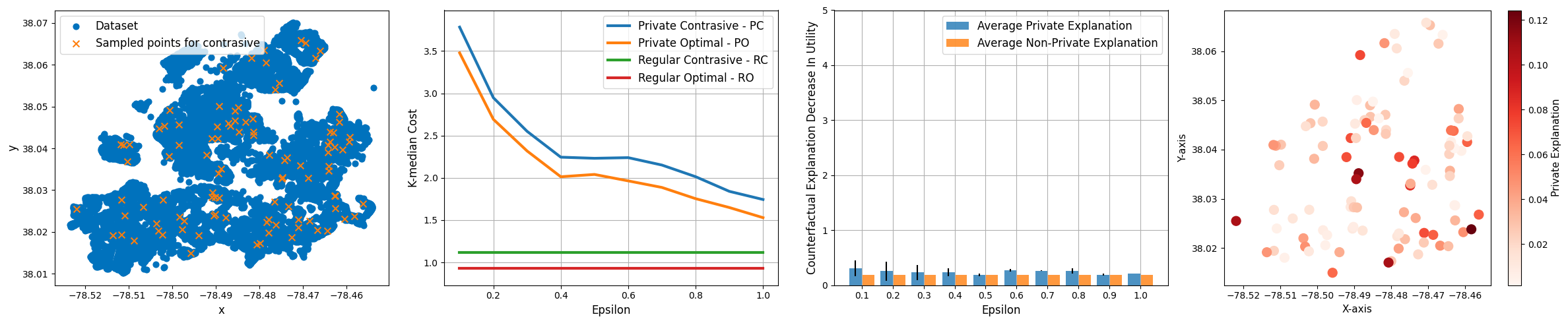
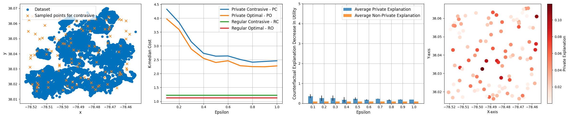
Beyond the Albemarle County dataset discussed in the main body of the paper, we also conducted experiments on other datasets, including the Charlottesville city dataset and synthetic activity-based populations. Here, we provide a detailed analysis of these experiments.

Charlottesville City Dataset:

This dataset is part of the synthetic U.S. population, as described in Chen et al. [2021], Barrett et al. [2009]. It comprises about 33K individuals and approximately 5600 activity locations visited by these individuals. The locations represent places where individuals perform various activities.

Synthetic 2D Dataset:

The synthetic dataset was meticulously crafted to emulate the distribution and characteristics of real-world datasets, ensuring a balance between realism and controlled variability. Comprising 100 data points in a 2D space, this dataset was uniformly distributed, mirroring the range observed in the real datasets we analyzed.

The primary motivation behind this synthetic dataset is to provide a sandbox environment, free from the unpredictable noise and anomalies of real-world data. This controlled setting is pivotal in understanding the core effects of differential privacy mechanisms, isolating them from external confounding factors. The dataset serves as a foundational tool in our experiments, allowing us to draw comparisons and validate our methodologies before applying them to more complex, real-world scenarios.

D.3.2 Experimental Results

Impact of $\epsilon$ on Private Optimal (PO) and Private Contrastive (PC):

For the Charlottesville city dataset, we observed similar trends to those in the Albemarle county dataset. As the $\epsilon$ value increased, prioritizing accuracy, there was a slight compromise in privacy. However, consistent with our hypothesis, the influence of the epsilon budget on the explainability of our outcomes was negligible.

Effect of Privacy on Explainability:

The contrastive explanations for the Charlottesville city dataset also showcased the resilience of our approach. Even with differential privacy perturbations, the quality of explanations remained consistent, emphasizing the robustness of our method.

Visualization:

Figure 2 - (a) showcases the Charlottesville city dataset. Blue dots represent the original dataset, while orange ’X’ markers indicate the sampled points for contrastives. The distribution of these points provides a visual representation of the data’s diversity and the regions we focused on for our contrastive analysis.

D.3.3 Performance Evaluation:

For each $\epsilon$ value, we conducted 25 different runs on the Charlottesville city dataset. The average results were consistent with our findings from the Albemarle County dataset. It’s essential to note that these multiple invocations were solely for performance evaluation. In real-world applications, invoking private algorithms multiple times could degrade the privacy guarantee.

Consistency in Contrastive Explanations across Datasets:

Despite the distinct scales between the Charlottesville city and the Albemarle county datasets, we observed consistent patterns in the contrastive explanations. Specifically, as illustrated in Figure 2 - (b) and Figure 2 - (c), the contrastive explanations remained largely unaffected by variations in the $\epsilon$ budget. This consistency further reinforces our hypothesis that the epsilon budget has a negligible influence on the explainability of our outcomes, even when applied to datasets of different scales.

Impact of Fixed Centroids on Contrastive Error:

In Figure 2 - (d), we delve deeper into the effects of selecting different centroids as fixed centroids. It’s evident that the choice of a fixed centroid has a pronounced impact on the contrastive error. This underscores the importance of the centroid’s position concerning the data distribution. Some centroids, especially those closer to data-dense regions, tend to produce lower counterfactual errors, while others, particularly those near sparser regions or outliers, result in higher errors. This observation highlights the intricate relationship between centroid positioning and the resulting contrastive explanation’s accuracy.

D.3.4 Conclusion:

The extended experiments on the Charlottesville city dataset further validate our approach’s efficacy. The balance between privacy and utility, the robustness of contrastive explanations, and the negligible impact of $\epsilon$ on explainability were consistent across datasets. These findings underscore the potential of our method for diverse real-world applications.

Contrastive explainable clustering with differential privacy

Abstract

1 Introduction

2 Related Work

3 Preliminaries

Definition 1.

Definition 2.

Definition 3.

Definition 4.

Definition 5.

Definition 6.

4 peCluster Mechanism

Theorem 1.

Lemma 1.

Theorem 2.

Lemma 2.

4.1 NonPrivateApproxFC for kk-median

Lemma 3.

Proof.

Lemma 4.

Proof.

Theorem 3.

Proof.

Corollary 1.

4.2 NonPrivateApproxFC for kk-means

Definition 7.

Definition 8.

Theorem 4.

Lemma 5.

Lemma 6.

Corollary 2.

5 Experiments

6 Discussion

References

Appendix A Related work: additional details

Appendix B Additional proofs for PECluster

Theorem 5.

Proof.

Lemma 7.

Proof.

Lemma 8.

Proof.

Lemma 9.

Lemma 10.

Theorem 6.

Proof.

Appendix C Additional proofs for kk-median algorithm

Definition 9.

Lemma 11.

Proof.

Lemma 12.

Lemma 13.

Appendix D Additional proofs for kk-means algorithm

Lemma 14.

Lemma 15.

Proof.

Lemma 16.

Lemma 17.

Proof.

D.1 Swap pairs mapping

D.2 γ\gamma-approximate candidate center set for fixed-center kk-means.

Definition 10.

Definition 11.

Lemma 18.

Theorem 7.

Proof.

D.3 Additional details on experiments

D.3.1 Datasets and Experimental Setup

Charlottesville City Dataset:

Synthetic 2D Dataset:

D.3.2 Experimental Results

Impact of ϵ\epsilon on Private Optimal (PO) and Private Contrastive (PC):

Effect of Privacy on Explainability:

Visualization:

D.3.3 Performance Evaluation:

Consistency in Contrastive Explanations across Datasets:

Impact of Fixed Centroids on Contrastive Error:

D.3.4 Conclusion:

4.1 NonPrivateApproxFC for $k$ -median

4.2 NonPrivateApproxFC for $k$ -means

Appendix C Additional proofs for $k$ -median algorithm

Appendix D Additional proofs for $k$ -means algorithm

D.2 $\gamma$ -approximate candidate center set for fixed-center $k$ -means.

Impact of $\epsilon$ on Private Optimal (PO) and Private Contrastive (PC):