Contrastive Learning from Spatio-Temporal Mixed Skeleton Sequences for Self-Supervised Skeleton-Based Action Recognition
Abstract
Self-supervised skeleton-based action recognition with contrastive learning has attracted much attention. Recent literature shows that data augmentation and large sets of contrastive pairs are crucial in learning such representations. In this paper, we found that directly extending contrastive pairs based on normal augmentations brings limited returns in terms of performance, because the contribution of contrastive pairs from the normal data augmentation to the loss get smaller as training progresses. Therefore, we delve into hard contrastive pairs for contrastive learning. Motivated by the success of mixing augmentation strategy which improves the performance of many tasks by synthesizing novel samples, we propose SkeleMixCLR: a contrastive learning framework with a spatio-temporal skeleton mixing augmentation (SkeleMix) to complement current contrastive learning approaches by providing hard contrastive samples. First, SkeleMix utilizes the topological information of skeleton data to mix two skeleton sequences by randomly combing the cropped skeleton fragments (the trimmed view) with the remaining skeleton sequences (the truncated view). Second, a spatio-temporal mask pooling is applied to separate these two views at the feature level. Third, we extend contrastive pairs with these two views. SkeleMixCLR leverages the trimmed and truncated views to provide abundant hard contrastive pairs since they involve some context information from each other due to the graph convolution operations, which allows the model to learn better motion representations for action recognition. Extensive experiments on NTU-RGB+D, NTU120-RGB+D, and PKU-MMD datasets show that SkeleMixCLR achieves state-of-the-art performance. Codes are available at https://github.com/czhaneva/SkeleMixCLR.
Index Terms:
Self-supervised learning, contrastive learning, hard contrastive pairs, skeleton-based action recognition.I Introduction
As a critical problem in computer vision, human action recognition has been researched for decades, since this task enjoys various applications, such as video surveillance, human-machine interaction, virtual reality, video analysis, and so on [1, 2, 3, 4, 5]. With the fast development of the depth sensors [6] and advanced pose estimation algorithm [7, 8, 9], 3D skeleton data becomes more accessible, making skeleton-based action recognition an essential branch in studying human action dynamics. In the past decades, skeleton-based action recognition has evolved by leaps and bounds, and many promising methods have emerged [10, 11, 12, 13, 14, 15, 16]. However, most of these methods follow a fully supervised framework, which requires numerous expensive annotated data. Therefore, self-supervised skeleton-based action recognition, which utilizes large amounts of unlabeled data to guide models to learn discriminative spatio-temporal motion representations, has emerged as a new popular research branch.
Several self-supervised works focus on designing pretext tasks, such as sequence reconstruction [17], jigsaw puzzle [18], or motion prediction [19], to help the model learn generalized features. Nevertheless, the joint-level pretext tasks require the model to learn fine-grained features invariant to viewpoint changes and skeleton scale, rather than focusing on higher-level semantic features relevant to skeleton-based action recognition. Recently, contrastive learning has become a key component of component self-supervised skeleton-based action recognition [20, 21, 22]. Contrastive learning based methods typically apply data augmentation on the skeleton sequences to generate different views of sequences and construct contrastive pairs between different views, then guide the model to learn spatio-temporal representations by pulling the positive pairs closer and pushing the negative samples away using a contrastive loss. Compared with the joint-level pretext tasks, contrastive learning based methods focus more on high-level context information, making the learned representations better for the downstream tasks.
The literature shows that augmentation and large sets of contrastive pairs play crucial roles in learning such representations [23, 24, 25]. Based on this, we try to improve contrastive learning by providing more contrastive pairs. However, as found in our experiments, naively extending contrastive pairs based on normal augmentations brings limited returns in terms of performance, because the contrastive pairs from the normal data augmentation contribute less and less to the loss as training progresses.
Considering that the contrastive pairs from the normal data augmentation provide insufficient information, which limits the ability to explore novel movement patterns, we therefore delve into hard contrastive pairs. At the same time, mixing augmentation strategy improves performance of many top-performing methods in various tasks by synthesizing novel samples, forcing the model to learn generalized and robust features [26, 27, 28, 29, 30]. Motivated by the above, we propose SkeleMixCLR: a contrastive learning framework with a spatio-temporal skeleton mixing augmentation (SkeleMix) to complement current contrastive learning approaches by providing hard contrastive samples. First, we propose a unique skeleton sequence augmentation strategy called SkeleMix for contrastive learning. Specifically, skeleton joints are first partitioned into five parts based on the topological information of skeleton data, and several body parts are randomly selected for cropping. Then, the cropped skeleton fragments (the trimmed view) are randomly combined with the remaining skeleton sequences (called the truncated view) to mix skeleton sequences. Second, we use a spatio-temporal mask pooling (STMP) operation to separate the trimmed and truncated views and get the embeddings of the corresponding views. Since the trimmed and truncated views share some context information from each other, they provide hard samples for contrastive learning. Finally, we combine our method with the baseline method SkeletonCLR [22] as SkeleMixCLR, and follow the general approach to construct contrastive pairs, i.e., each view is positive with the views augmented from the same original skeleton sequences and negative with views augmented from other skeleton sequences [23, 24]. Moreover, we propose to perform multiple SkeleMix augmentation to provide diverse hard samples (SkeleMixCLR+), which can further boost the performance. Our method enables the model to learn better local and global spatio-temporal action representations by utilizing the mixed skeleton sequences to provide plenty of hard positive pairs such as the truncated view and the key view (as well as the trimmed view and the key view), and hard negative pairs such as the trimmed view and the truncated view, which helps to extract generalized representations for downstream tasks.
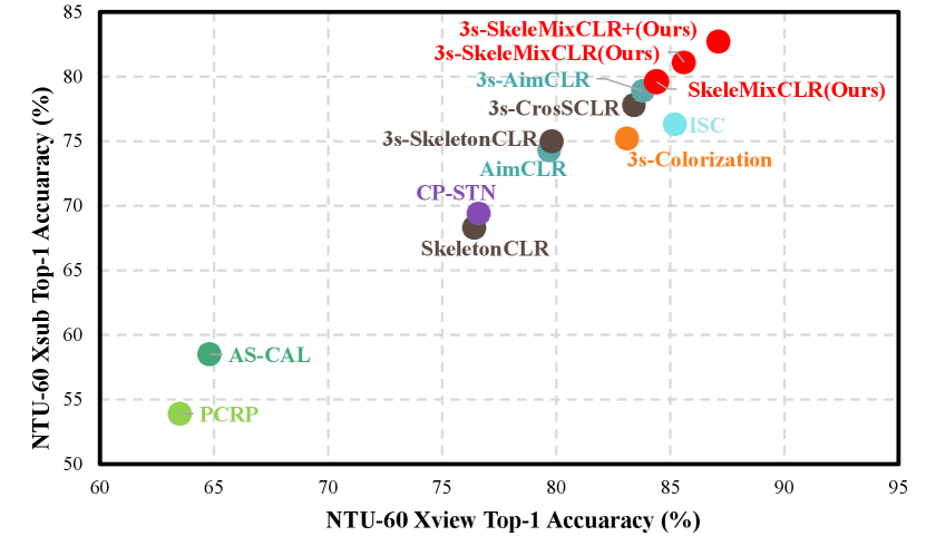
Figure 1 shows the superiority of our proposed method. SkeleMixCLR substantially improves the baseline SkeletonCLR by on NTU-RGB+D benchmark [31]. The single stream SkeleMixCLR outperforms many other methods, such as PCRP [32], AS-CAL [20], CP-STN [33], ISC [34], and even some ensemble methods, such as 3s-CrosSCLR [22], 3s-AimCLR [21], and 3s-Colorization [35]. Our contributions can be summarized as follows:
-
•
We propose SkeleMix augmentation to provide abundant hard samples for self-supervised skeleton-based action recognition by combining the topological information of skeleton data.
-
•
A simple yet effective framework SkeleMixCLR based on SkeleMix is proposed. The SkeleMixCLR facilitates the model to learn better discriminative global and local representations by introducing extensive hard contrastive pairs, which helps to achieve better performance in downstream tasks.
-
•
A multiple SkeleMix augmentation strategy is proposed to provide diverse hard samples, which can further boost the performance.
-
•
Extensive experimental results on NTU-RGB+D, NTU120-RGB+D, and PKU-MMD datasets show that the proposed SkeleMixCLR achieves state-of-the-art performance under a variety of evaluation protocols.
II Related Work
II-A Self-Supervised Contrastive Learning
Contrastive learning, whose goal is increasing the similarity between positive pairs and decreasing the similarity between negative pairs, has shown promising performance in self-supervised representation learning [23, 24]. In the past few years, there emerged numerous self-supervised representation learning works based on contrastive learning, such as instance discrimination [36], SwAv [37], MoCo [23], SimCLR [24], BYOL [38], contrastive cluster [39], DINO [40], and SimSiam [41]. These methods have achieved advanced results and are easy to transfer to other areas, such as skeleton-based action recognition. In this paper, we follow MoCov2 [42] framework to implement our method.
II-B Mixing Augmentation Strategy
Most of the top-performing contrastive methods leverage data augmentations, which is crucial in learning useful representations because they modulate the hardness of the self-supervised task via the contrastive pairs. Recently, Mixing [26] and CutMix [27] are widely discussed in self-supervised contrastive learning. These operations are mainly performed between embedding features or between samples. MoCHi [25] proposes a hard negative mixing strategy, which generates hard negative samples by mixing the embedding features to improve the generalization of the learned visual representations. Vi-Mix [43] proposes CMMC to mix the data across different modalities of a video in their intermediate representations. MixCo [44], Un-Mix [45] and i-Mix [46] perform mixing operation between samples and generate corresponding smoothing labels to let the model be aware of the soft degree of similarity between contrastive pairs. The above methods mainly construct contrastive pairs with the mixing features. Different from these methods, we utilize the features of the trimmed and truncated views separated by STMP to provide hard samples for contrastive learning. Our method not only makes better use of the augmented features, but also improves the ability of the model to learn both local and global representations. RegionCL [47] also propose to utilize the separated features, while our method leverages the topological information of the skeleton data to maintain the consistency of action information, and performs mixing operation on both spatial and temporal domain. Moreover, we propose to apply multiple SkeleMix operation to provide a more adequate hard contrastive pairs.
II-C Self-Supervised Skeleton-Based Action Recognition
Self-supervised skeleton-based action recognition has emerged as one of the promising direction for action recognition. LongT GAN [17] and P&C [48] rely on regeneration of the skeleton sequences to help the model to learn spatio-temporal representations. Colorization [35] leverages the colorized skeleton point cloud and designs an auto-encoder framework that can effectively learn spatio-temporal features from the artificial color labels of skeleton joints. With the development of contrastive learning, the past few years have witnessed a surge of successful self-supervised contrastive skeleton-based action recognition. AS-CAL [20] exploits eight different skeleton sequence augmentations and their combinations to generate query and key views for contrastive learning. ISC [34] proposes inter-skeleton contrastive learning to enhance the learned features via different input skeleton representations. MS2L [18] and CP-STN [33] combine contrastive learning with multi-pretext tasks such as masked sequences prediction, enabling the model to fully extract discriminative representations with spatio-temporal information. Works like CrosSCLR [22] and AimCLR [21] also try to improve contrastive learning by introducing extra hard contrastive pairs. In CrosSCLR, a cross-view knowledge mining strategy is developed to exam the similarity of samples, and select the most similar pairs as positive ones to boost the positive set in complementary views. In AimCLR, an extreme augmentation strategy is proposed to introduce movement patterns, which forces the model to learn more general representations by providing harder contrastive pairs. In this paper, we propose a unique skeleton sequence augmentation strategy SkeleMix to provide hard contrastive samples, which guides the model to learn better local and global spatio-temporal representations.
III Methodology
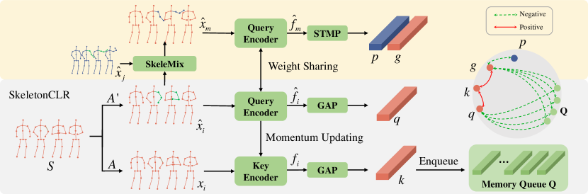
III-A Overview of SkeletonCLR
As illustrated in the gray box of Figure 3, SkeletonCLR [22] follows the MoCov2 framework [42] to learn skeleton-based action representations. Given a skeleton sequence , two different augmentations and are applied to to obtain query sample and key sample . We denote , where , , and are the number of channels, frames, and nodes, respectively. A query encoder and a momentum updated key encoder followed by global average pooling (GAP) are used to get query embedding and key embedding . Then the key embedding is stored in a first-in-first-out memory queue , where denotes the queue size. Following the criteria for constructing contrastive pairs in MoCov2, and form positive pairs while and the embeddings in Q form negative pairs. The InfoNCE loss [49] formulated as Eq. (1) is used to train the network, where is dot product to compute the similarity between two normalized embeddings, and is the temperature hyperparameter (set to 0.2 by default). denotes the similarity between embeddings of view and memory queue Q.
| (1) |
The parameters of query encoder are updated via gradient back propagation while the parameters of key encoder are updated as a moving-average of the query encoder, which can be formulated as:
| (2) |
where is a momentum coefficient and typically close to 1 to maintain consistency of the embeddings in the memory queue.
III-B SkeleMix Augmentation
In this section, we will introduce our SkeleMix augmentation, which is a spatio-temporal mixing augmentation strategy.
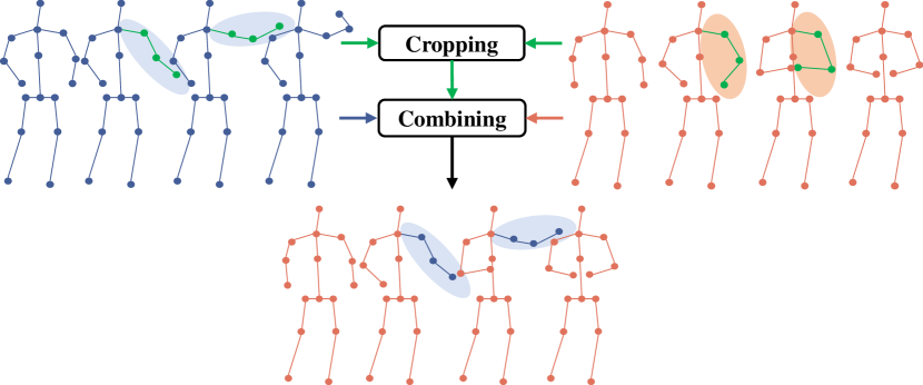
As illustrated in Figure 2, our SkeleMix follows CutMix to peroform spatio-temporal mixing on skeleton sequences.
Specifically, in the cropping step, skeleton joints are first partitioned into five part subsets left-hand, right-hand, left-leg, right-leg, trunk based on the topological information of skeleton data.
Second, two discrete uniform distributions and are used to determine the number of body parts to crop out and the duration of the cropped skeleton fragments.
We sample once in each training iteration and obtain and .
Then, we randomly choose body parts from to get the cropped skeleton joints , and randomly sample the start frame from a valid range that guarantees the completeness of the cropped skeleton fragments.
Combining and , we can obtain the corresponding temporal cropping region .
Finally, we perform spatio-temporal cropping operation on to get the cropped skeleton fragments.
It is notable that the cropped regions ( and ) within a mini-batch of the training skeleton sequences are typically the same to maintain consistency of action information.
In combining step, we randomly combine the cropped skeleton fragments (named as the trimmed view) and the remaining skeleton sequences (named as the truncated view) to generate the mixed skeleton sequences.
Thus, the mixed skeleton sequences consist of the trimmed view and truncated view.
Furthermore, to provide a sufficient hard samples for contrastive learning, we propose to perform multiple SkeleMix augmentation.
For convenience, we denote the mixed skeleton sequences generated by the SkeleMix augmentation as , where denotes the total number of SkeleMix augmentation performed.
III-C SkeleMixCLR
In this section, we introduce our SkeleMixCLR in detail. A weight-sharing encoder with the query view in SkeletonCLR [22] is used to extract features from the mixed skeleton sequences . We denote , where is the feature dimension and where is the temporal downsampling ratio of the model. To separate the embedding of the trimmed view and the truncated view , we utilize a spatio-temporal mask pooling operation (STMP), which can be formulated as:
| (3) | ||||
where is a [0, 1] mask indicates the corresponding cropped skeleton fragments, while indicates the corresponding remaining skeleton sequences. I is unit matrix with shape . Then, we extend the contrastive pairs with the trimmed view and the truncated view. Following the criteria of constructing contrastive pairs in MoCov2 [42], for the trimmed embedding , it is positive with corresponding key embeddings while negative with and the embeddings stored in the memory bank Q. Therefore, the contrastive loss for the trimmed view can be written as:
| (4) |
Similarly, the truncated embedding is positive with corresponding key embeddings , while negative with and the embeddings store in the memory bank Q. Therefore, the contrastive loss for the truncated view can be written as:
| (5) |
Since the trimmed view and the truncated view share context information during forward inference, and the action information they contain is incomplete, they provide hard samples for contrastive learning. The expanded contrastive samples provide extensive hard positive pairs such as and (as well as and ) and hard negative pairs such as and , thus helping the model to learn better global and local spatio-temporal representations and improving the performance in downstream tasks.
Considering that the trimmed view and the truncated view are symmetrical, we use the average of and as the overall loss of the mix branch, which can formulated as:
| (6) |
Finally, the loss used to optimize the encoder can be formulated as:
| (7) |
where is a hyperparameter to balance the easy contrastive pairs and the hard contrastive pairs.
IV Experiments
IV-A Datasets
In order to evaluate the effectiveness of the proposed method, we conduct experiments on three widely used datasets for skeleton-based action recognition.
NTU RGB+D [31], denoted as NTU-60, is the most widely used dataset for skeleton-based action recognition. It contains 60 action classes and 56,578 action instances which are performed by 40 performers. We follow the recommended evaluation protocols cross-subject (Xsub) and cross-view (Xview) to evaluate our method.
NTU RGB+D 120 [50], denoted as NTU-120, is the expansion of NTU RGB+D dataset in the number of performer and action categories. The scale of this dataset is improved to 120 action classes and 113,945 action instances. Two recommended evaluation protocols, cross-subject (Xsub) and cross-set (Xset) are used to evaluate our method.
PKU-MMD [51] contains almost 20,000 action instances and 51 action classes. It consists of two subsets, where part II is more challenging than part I due to more noise caused by view variation. We evaluate our method on cross-subject benchmark of both subsets.
IV-B Experiments Settings
To perform a fair comparison, we use the same data pre-processing with SkeletonCLR [22] and AimCLR [21] except for that we resize the length of skeleton sequences to 64 frames, rather than 50 frames. This allows our SkeleMix to be implemented more efficiently, since the temporal downsample ratio is 4 of ST-GCN backbone. Thus, the temporal size of the final output feature is 16. The batch size for both pretraining and downstream tasks is set to 128 for by default, except in specific cases.
Data Augmentation. For skeleton sequence, a spatial augmentation together with a temporal augmentation is adopted to generate the query and key views. and use the same combination of augmentations but with different parameters due to the randomness.
(1) : The shear augmentation is a linear transformation on the spatial dimension. The shape of 3D coordinates of body joints is slanted with a random angle. The transformation matrix is defined as:
| (8) |
where , , , , , are shear factors that randomly sampled from a uniform distribution , where is the shear amplitude. Follow SkeletonCLR and AimCLR, we set . The skeleton sequence is multiplied by the transformation matrix on the channel dimension.
(2) : For the temporal skeleton sequence, specifically, we symmetrically pad some frames to the sequence and then randomly crop it to the original length, which increases the diversity while maintaining the distinction of original samples. The padding length is defined as , where is the padding ratio and here we set .
Self-Supervised Pretext Training. The baseline method of our SkeleMixCLR is SkeletonCLR which follows the MoCov2 framework [42]. Therefore, the hyperparameters queue size , temperature in MoCov2 are important. In SkeletonCLR, and , while we found that and is a better choice under our experiments settings. In most cases, our reproduction performs better than the original results reported on [22]. Thus, we use the results of our reproduction as our baseline. For the backbone, we adopt ST-GCN [11], but reduce the number of channels in each layer to 1/4 of the original settings and the final feature dimension is set to 128. For the optimizer, we use SGD with momentum (0.9) and weight decay (0.0001). The model is trained for 300 epochs with a learning rate of 0.1. The model is trained for 300 epochs with a learning rate of 0.1. For fair comparison, we also use three streams of skeleton sequences, i.e., joint, motion, and bone denoted as J, M, and B, respectively. The ensemble results are obtained from the score-level fusion with equal weights.
IV-C Evaluation Protocol
We compare our method with other methods under a variety of evaluation protocols, including KNN evaluation protocol, linear evaluation protocol, finetune protocol, and semi-supervised evaluation protocol.
KNN Evaluation Protocol. A k-nearest neighbor (KNN) classifier without trainable parameters is used on the features extracted from the trained encoder. For all reported KNN results, , and the temperature is set to 0.1. The results reflect the quality of the features learned by the encoder.
Linear Evaluation Protocol. This is the most commonly used protocol for classification downstream task. Specifically, we append a classification head (a fully connected layer together with a softmax layer) after the pretrained encoder and train the network with the encoder fixed. An SGD with an initial learning rate of 3.0 is used to train the network for 100 epochs.
Finetune Protocol. We append a linear classification head to the pretrained encoder. And then, we use an SGD optimizer with initial learning rate (0.1), weight decay (0.0001) to train the whole network for 110 epochs. The learning rate is decayed by 10 at the , the , and the epoch. We also use 10-epoch warmup to improve the stability of the training process.
Semi-Supervised Evaluation Protocol. This protocol follows the same settings as finetune protocol except for the scale of training datasets. Only 1% or 10% randomly selected labeled data are used to finetune the whole network. On PKU-MMD Part II benchmark with 1% labeled data, the batch size is set to 52, due to the limited data. An SGD with an initial learning rate of 0.1 (decreases by 10 at epoch) is used to optimize the whole network for 100 epochs. We also use 20-epoch warmup to improve the stability of the training process.
IV-D Ablation Study
In this section, we conduct ablation studies on different datasets with linear evaluation protocol to verify the effectiveness of different components of our method.
| Method | Stream | NTU-60(%) | PKU-MMD(%) | NTU-120(%) | |||||||||
|---|---|---|---|---|---|---|---|---|---|---|---|---|---|
| Xsub | Xview | part I | part II | Xsub | Xset | ||||||||
| acc. | acc. | acc. | acc. | acc. | acc. | ||||||||
| SkeletonCLR [22] | J | 68.3 | 76.4 | 80.9 | 35.2 | 56.8 | 55.9 | ||||||
| SkeletonCLR† [22] | J | 74.8 | +6.5 | 78.9 | +2.3 | 81.1 | +0.2 | 35.8 | +0.6 | 63.2 | +6.4 | 58.9 | +3.0 |
| SkeleMixCLR (Ours) | J | 79.6 | +11.3 | 84.4 | +8.0 | 89.2 | +8.3 | 51.6 | +16.4 | 67.4 | +10.6 | 69.6 | +13.7 |
| SkeleMixCLR+ (Ours) | J | 80.7 | +12.4 | 85.5 | +9.1 | 88.1 | +7.2 | 55.0 | +19.8 | 69.0 | +12.2 | 68.2 | +12.3 |
| SkeletonCLR [22] | M | 53.3 | 50.8 | 63.4 | 13.5 | 39.6 | 40.2 | ||||||
| SkeletonCLR† [22] | M | 49.6 | -3.7 | 53.6 | +2.8 | 63.9 | +0.5 | 16.8 | +3.3 | 41.3 | +1.7 | 44.1 | +3.9 |
| SkeleMixCLR (Ours) | M | 70.3 | +17.0 | 76.1 | +25.3 | 81.5 | +18.1 | 32.1 | +18.6 | 49.7 | +10.1 | 53.8 | +13.6 |
| SkeleMixCLR+ (Ours) | M | 74.1 | +20.8 | 74.8 | +24.0 | 83.8 | +20.4 | 32.4 | +18.9 | 48.5 | +8.9 | 50.5 | +10.3 |
| SkeletonCLR [22] | B | 69.4 | 67.4 | 72.6 | 30.4 | 48.4 | 52.0 | ||||||
| SkeletonCLR† [22] | B | 70.3 | +0.9 | 72.4 | +5.0 | 80.0 | +7.4 | 25.0 | -5.4 | 54.2 | +5.8 | 58.7 | +6.7 |
| SkeleMixCLR (Ours) | B | 76.3 | +6.9 | 82.0 | +14.6 | 89.0 | +16.4 | 41.8 | +11.4 | 67.1 | +18.7 | 63.1 | +11.1 |
| SkeleMixCLR+ (Ours) | B | 79.1 | +9.7 | 82.6 | +15.2 | 89.1 | +16.5 | 46.0 | +15.6 | 63.0 | +14.6 | 60.7 | +8.7 |
| 3s-SkeletonCLR [22] | J+M+B | 75.0 | 79.8 | 85.3 | 40.4 | 60.7 | 62.6 | ||||||
| 3s-SkeletonCLR† [22] | J+M+B | 75.9 | +0.9 | 79.8 | 0.0 | 85.4 | +0.1 | 37.6 | -2.8 | 65.0 | +4.3 | 65.9 | +3.3 |
| 3s-SkeleMixCLR (Ours) | J+M+B | 81.0 | +6.0 | 85.6 | +5.8 | 90.6 | +5.3 | 52.9 | +12.5 | 69.1 | +8.4 | 69.9 | +7.3 |
| 3s-SkeleMixCLR+ (Ours) | J+M+B | 82.7 | +7.7 | 87.1 | +7.3 | 91.1 | +5.8 | 57.1 | +16.7 | 70.5 | +9.8 | 70.7 | +8.1 |
Comparisons with SkeletonCLR. We conduct experiments on NTU-60, NTU-120, and PKU-MMD datasets to compare our method with baseline method SkeletonCLR in detail. As can be seen from Table I, the reproduced SkeleMixCLR with our settings achieves better performance than the original one, so we use the reproduced one as our baseline for fair comparison. Moreover, our SkeleMixCLR substantially improves SkeletonCLR, especially for the motion stream and bone stream. Multiple SkeleMix augmentation strategy could further boost the performance, and 3s-SkeleMixCLR+ achieves the best performance compared with SkeletonCLR and 3s-SkeleMixCLR. The experimental results demonstrate the effectiveness of our proposed method.
Choice of Cropped Skeleton Fragments. There are four hyperparameters (, , , and ) introduced by our method. To determine them, we first fix and , and try all the valid combinations between and . As show in Table II, we found that the best setting is and . Then we fix the best combination of , , and to search for the best . Finally, we search for the best with other three parameters fixed. Based on the results shown in Table II, we choose , , , and as our default setting to perform SkeleMix augmentation.
| NTU-60-J (%) | ||||||
|---|---|---|---|---|---|---|
| Xsub | Xview | Avg | ||||
| - | - | - | - | 74.8 | 78.9 | 76.9 |
| 1 | 1 | 5 | 11 | 78.2 | 80.6 | 79.4 |
| 1 | 2 | 5 | 11 | 79.2 | 79.8 | 79.5 |
| 1 | 3 | 5 | 11 | 78.1 | 81.7 | 79.9 |
| 1 | 4 | 5 | 11 | 77.8 | 79.7 | 78.8 |
| 2 | 2 | 5 | 11 | 77.8 | 83.1 | 80.5 |
| 2 | 3 | 5 | 11 | 78.8 | 84.2 | 81.5 |
| 2 | 4 | 5 | 11 | 78.0 | 83.9 | 81.0 |
| 3 | 3 | 5 | 11 | 76.6 | 83.8 | 80.2 |
| 3 | 4 | 5 | 11 | 78.3 | 83.2 | 80.8 |
| 4 | 4 | 5 | 11 | 77.2 | 82.4 | 79.8 |
| 2 | 3 | 1 | 11 | 77.8 | 82.4 | 80.1 |
| 2 | 3 | 3 | 11 | 80.4 | 82.0 | 81.2 |
| 2 | 3 | 5 | 11 | 78.8 | 84.2 | 81.5 |
| 2 | 3 | 7 | 11 | 79.6 | 84.4 | 82.0 |
| 2 | 3 | 9 | 11 | 79.0 | 83.1 | 81.1 |
| 2 | 3 | 7 | 7 | 79.9 | 82.9 | 81.4 |
| 2 | 3 | 7 | 9 | 79.8 | 84.0 | 81.9 |
| 2 | 3 | 7 | 11 | 79.6 | 84.4 | 82.0 |
| 2 | 3 | 7 | 13 | 79.3 | 83.4 | 81.4 |
| 2 | 3 | 7 | 15 | 79.3 | 83.0 | 81.2 |
Balance Easy Contrastive Pairs and Hard Contrastive Pairs. In our model, we present that the power of easy contrastive pairs and hard contrastive pairs are traded by a hyperparameter . Here, we analyze how affects the performance of the model. For convenience, we set , and compare the performance of different on NTU-60 dataset with linear evaluation protocol. From Table III, when , the model get the highest recognition accuracy, showing large improvements than cases with and . Therefore, we set as default setting.
| NTU-60-J (%) | |||
|---|---|---|---|
| Xsub | Xview | Avg | |
| 0.1 | 75.1 | 81.3 | 78.2 |
| 1.0 | 79.6 | 84.4 | 82.0 |
| 10.0 | 83.0 | 76.8 | 79.9 |
| Method | 100ep | 200ep | 300ep | |
|---|---|---|---|---|
| Xview | SkeletonCLR† [22] | 75.5 | 77.8 | 78.9 |
| SkeleMixCLR (Ours) | 81.3 | 83.5 | 84.4 | |
| Xsub | SkeletonCLR† [22] | 71.1 | 73.9 | 74.8 |
| SkeleMixCLR (Ours) | 78.2 | 79.3 | 79.6 | |
Training with Different Epochs. We also investigate the influence of different training epochs. The results are shown in Table IV, as we can see that all methods are close to convergence, thus we believe that 300 epochs are sufficient for comparing. Our method outperforms the baseline method SkeletonCLR with all settings of different training epochs. It is worth mentioning that with only 100 training epochs, the proposed SkeleMixCLR outperforms SkeletonCLR with 300 training epochs. The results not only show good property of convergence brought by SkeleMixCLR, but also verify that our method can enhance the representation capacity of the model with more training epochs.
Effectiveness of Proposed SkeleMix Strategy. Our SkeleMix augmentation strategy utilizes the topological information to perform skeleton sequence mixing operation, which not only makes better use of the augmented data, but also maintains the consistency of action information, thus providing more reasonable and informative features for contrastive learning. To validate the efficiency of our method, we compare SkeleMix with zeros padding strategy, which pads zeros to the remaining skeleton sequences. The comparisons are shown in Table VI. Zeros padding strategy slightly improves the performance, while a big improvement by has been achieved with our SkeleMix. The results demonstrate that our SkeleMix augmentation can make full use of the augmented skeleton sequences to provide more informative features for contrastive learning. Moreover, different from images, skeleton data contains topological information and our method utilizes such information to perform part-level mixing operation which maintains the consistency of both remaining skeleton sequences and cropped skeleton fragments. To verify the efficiency of the topological information, we compare our method with the random strategy, which randomly selects some skeleton joints to crop. From Table VI, our method outperforms the random strategy especially on NTU-60 Xivew benchmark, which demonstrates the effectiveness of the topological information and our method can make good use of such information to help the model learn better spatio-temporal representations.
| NTU-60-J | Xsub | Xview |
|---|---|---|
| Baseline | 74.8 | 78.9 |
| Zeros | 76.2 | 81.1 |
| SkeleMix | 79.6 | 84.4 |
| NTU-60-J | Xsub | Xview |
|---|---|---|
| Baseline | 74.8 | 78.9 |
| Random | 77.7 | 80.2 |
| Topology | 79.6 | 84.4 |
| Xsub | Xview | |||||
|---|---|---|---|---|---|---|
| ✗ | ✗ | ✗ | ✗ | ✗ | 74.8 | 78.9 |
| ✓ | 75.2 | 79.4 | ||||
| ✓ | 78.4 | 79.8 | ||||
| ✓ | 77.4 | 82.3 | ||||
| ✓ | ✓ | 79.1 | 82.4 | |||
| ✓ | ✓ | ✓ | 79.3 | 84.3 | ||
| ✓ | ✓ | ✓ | ✓ | 79.6 | 84.4 |
Effectiveness of Hard Contrastive Pairs.
Our method can provide abundant hard contrastive pairs in contrastive pretext task. To further verify the effectiveness of our method, we test the influence of each component. A blank control method (denoted as ) is constructed by naively extending a query view and constructing the corresponding contrastive pairs. The results are shown in Table VII, where and denote whether to use and to construct hard contrastive pairs, respectively. denotes whether to use and to construct hard negative pairs. Since SimSiam [41] further finds that stop-gradient is critical to prevent from collapsing, we also use this strategy denoted as when constructing hard negative pairs between and . As shown in Table VII, naively extending contrastive pairs based on normal augmentations brings limited returns in terms of performance (0.4% on Xsub benchmark and 0.5% on Xview benchmark), which indicates that more does not mean effective. Compared with the blank control method, we found that the hard positive pairs contribute a lot to the performance and using hard negative pairs also greatly improves the performance on NTU-60 Xview benchmark. The stop-gradient strategy can further improve the performance.
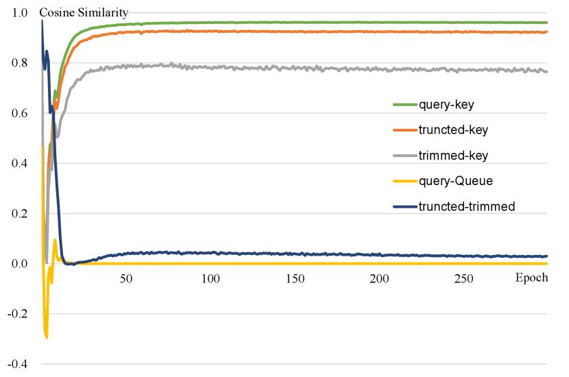
To further analyze our approach, we compare the average cosine similarity of easy contrastive pairs provided by baseline and hard contrastive pairs introduced by our method. As shown in Figure 4, as the training progresses, the cosine similarity between easy positive contrastive pairs (query and key) is very close to 1, and the cosine similarity between easy positive contrastive pairs (query and Queue) is very close to 0, which contribute less and less to the loss [25]. Hard positive contrastive pairs (truncated and key, trimmed and key) and hard negative contrastive pairs (truncated and trimmed) are harder than easy contrastive pairs, which contributes more to optimize the model.
To summarize the above, our method uses SkeleMix augmentation strategy to generate the mixed skeleton sequences and separate the trimmed view and the truncated view at the feature level to provide hard samples for contrastive learning. SkeleMixCLR further utilizes the hard samples to expand the contrastive pairs with hard positive pairs and hard negative pairs, which significantly improves the capacity of the model in learning better complete and discriminative spatio-temporal representations for skeleton-based action recognition.
| NTU-60-J (%) | |||
|---|---|---|---|
| Xsub | Xview | Avg | |
| 1 | 79.6 | 84.4 | 82.0 |
| 2 | 80.9 | 85.0 | 83.0 |
| 3 | 80.7 | 85.5 | 83.1 |
| 4 | 80.5 | 79.3 | 79.9 |
| Method | NTU-60 | NTU-120 | PKU-MMD | |||
|---|---|---|---|---|---|---|
| Xsub | Xview | Xsub | Xset | part I | part II | |
| SkeletonCLR† [22] | 64.8 | 60.7 | 41.9 | 42.9 | 64.9 | 19.9 |
| AimCLR† [21] | 71.0 | 63.7 | 48.9 | 47.3 | 73.2 | 19.4 |
| SkeleMixCLR (Ours) | 72.3 | 65.5 | 49.3 | 48.3 | 75.7 | 33.8 |
| Method | Xsub (%) | Xset (%) |
|---|---|---|
| Single-stream: | ||
| PCRP [32] | 41.7 | 45.1 |
| AS-CAL [20] | 48.6 | 49.2 |
| SkeletonCLR ([22]) | 56.8 | 55.9 |
| ISC [34] | 67.9 | 67.1 |
| AimCLR ([21]) | 63.4 | 63.4 |
| SkeleMixCLR (Ours) | 67.4 | 69.6 |
| SkeleMixCLR+ (Ours) | 69.0 | 68.2 |
| Multi-stream: | ||
| 3s-SkeletonCLR ([22]) | 60.7 | 62.6 |
| 3s-CrosSCLR ([22]) | 67.9 | 66.7 |
| 3s-AimCLR [21] | 68.2 | 68.8 |
| 3s-SkeleMixCLR+ (Ours) | 69.1 | 69.9 |
| 3s-SkeleMixCLR+ (Ours) | 70.5 | 70.7 |
Influence of The Multiple SkeleMix Augmentation Strategy As described in Sec. III-B and Sec. III-C, to provide a more adequate hard contrastive pairs, we propose to perform multiple SkeleMix augmentations. Here, we conduct experiments on NTU-60 datasets with linear evaluation protocol to analyze how affects the performance. As shown in Table VIII, when , the average performance over NTU-60 Xsub and Xview benchmarks is improved from 82.0 to 83.0. There is a slight improvement in average performance when increasing from 2 to 3. While increasing from 3 to 4 leads to a dramatic drop. We believe this is caused by the model focusing too much on hard contrastive pairs and destroying the balance between simple and hard contrastive pairs. Based on the above experiments, we set as the default setting.
IV-E Comparison with State-of-the-Art Methods
KNN Evaluation Protocol Results. We compare our SkeleMixCLR with SkeletonCLR and AimCLR on three datasets. The results are shown in Table IX, our SkeleMixCLR outperforms both methods by a large margin especially in relatively small dataset PKU-MMD, which shows that the features learned by SkeleMixCLR are more discriminative.
Linear Evaluation Protocol Results. Table X, XI, and XII show the comparisons on NTU-120, NTU-60, and PKU-MMD datasets with linear evaluation protocol, respectively. Notably, our single SkeleMixCLR outperforms some ensemble methods such as 3s-SkeletonCLR [22], 3s-Colorization [35], 3s-CrosSCLR [22], and 3s-AimCLR [21] on NTU-60, PKU-MMD, and NTU-120 Xset benchmarks. Multiple SkeleMix augmentation strategy could further boost the performance, achieving considerable gains on most benchmarks. It is worth mentioning that just with only single joint stream, our SkeleMixCLRor SkeleMixCLR+surpasses many multi-stream methods with a big margin. When multiple streams of information are introduced, our method can be further improved. On NTU-60, our 3s-SkeleMixCLR+ outperforms 3s-AimCLR by 3.8% on Xsub and outperforms ISC [34] by 1.9% on Xview. On NTU-120, our 3s-SkeleMixCLR+ outperforms 3s-AimCLR by 2.3% and 1.9% on Xsub and Xset, respectively. On PKU-MMD, our 3s-SkeleMixCLR+ outperforms 3s-AimCLR by a large margin (3.3% on part I and 18.6% on part II). Based on the above, our method performs well on both large scale and small scale datasets, which demonstrates the effectiveness and generalization of our method.
| Method | Xsub (%) | Xview (%) |
|---|---|---|
| Single-stream: | ||
| LongT GAN [17] | 39.1 | 48.1 |
| MS2L [18] | 52.6 | - |
| PCRP [32] | 53.9 | 63.5 |
| AS-CAL [20] | 58.5 | 64.8 |
| SkeletonCLR ([22]) | 68.3 | 76.4 |
| ISC [34] | 76.3 | 85.2 |
| AimCLR [21] | 74.3 | 79.7 |
| SkeleMixCLR (Ours) | 79.6 | 84.4 |
| SkeleMixCLR+ (Ours) | 80.7 | 85.5 |
| Multi-stream: | ||
| 3s-SkeletonCLR ([22]) | 75.0 | 79.8 |
| 3s-Colorization [35] | 75.2 | 83.1 |
| 3s-CrosSCLR ([22]) | 77.8 | 83.4 |
| 3s-AimCLR [21] | 78.9 | 83.8 |
| 3s-SkeleMixCLR (Ours) | 81.1 | 85.6 |
| 3s-SkeleMixCLR+ (Ours) | 82.7 | 87.1 |
| Method | part I (%) | part II (%) |
|---|---|---|
| Single-stream: | ||
| LongT GAN [17] | 67.7 | 26.0 |
| MS2L [18] | 64.9 | 27.6 |
| SkeletonCLR [22] | 80.9 | 35.2 |
| AimCLR [21] | 83.4 | 36.8 |
| ISC [34] | 80.9 | 36.0 |
| SkeleMixCLR (Ours) | 89.2 | 51.6 |
| SkeleMixCLR+ (Ours) | 88.1 | 55.0 |
| Multi-stream: | ||
| 3s-SkeletonCLR [22] | 85.3 | 40.4 |
| 3s-CrosSCLR ([22]) | 84.9 | 21.2 |
| 3s-AimCLR [21] | 87.8 | 38.5 |
| 3s-SkeleMixCLR (Ours) | 90.6 | 52.9 |
| 3s-SkeleMixCLR+ (Ours) | 91.1 | 57.1 |

Finetuned Evaluation Results. We compare our method with other self-supervised methods and some supervised methods, such as ST-GCN, which has all the same structure and parameters as ours. As shown in Table XIII, our 3s-SkeleMixCLR achieves better results than supervised 3s-ST-GCN and other self-supervised methods, which indicates the effectiveness of our method. Moreover, in most cases, SkeleMixCLR+performs better than SkeleMixCLR, which indicates that the proposed multiple SkeleMix augmentation strategy could further boost the performance.
Semi-Supervised Evaluation Results. With only 1% and 10% labeled data, the spatio-temporal representations learned by the model in the pretext task are important, because little data can lead to difficult convergence or overfitting problems. From Table XIV, our 3s-SkeleMixCLR+ outperforms other methods consistently for all configurations. The results indicate that our method can make better use of spatio-temporal information, which significantly helps the model to learn better spatio-temporal representations.
Based on the above experiments, we conclude that our method achieves state-of-the-art performance for self-supervised skeleton-based action recognition.
| Method | NTU-60 (%) | NTU-120 (%) | ||
|---|---|---|---|---|
| Xsub | Xview | Xsub | Xset | |
| Single-stream: | ||||
| SkeletonCLR‡ [22] | 82.2 | 88.9 | 73.6 | 75.3 |
| AimCLR‡ [21] | 83.0 | 89.2 | 77.2 | 76.0 |
| SkeleMixCLR (Ours)‡ | 84.5 | 91.1 | 75.1 | 76.0 |
| SkeleMixCLR+ (Ours)‡ | 84.7 | 91.8 | 76.7 | 78.4 |
| Multi-stream: | ||||
| 3s-ST-GCN§ [11] | 85.2 | 91.4 | 77.2 | 77.1 |
| 3s-CrosSCLR ([22]) | 86.2 | 92.5 | 80.5 | 80.4 |
| 3s-AimCLR [21] | 86.9 | 92.8 | 80.1 | 80.9 |
| 3s-SkeleMixCLR (Ours) | 87.8 | 93.9 | 81.6 | 81.2 |
| 3s-SkeleMixCLR+ (Ours) | 87.7 | 94.0 | 82.0 | 82.9 |
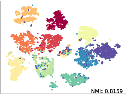
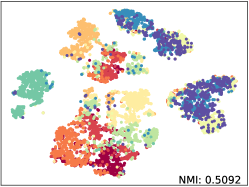
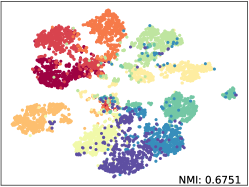
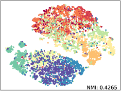
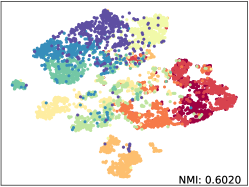
Qualitative Results. We apply t-SNE [52] with fixed settings to show the embeddings distribution of SkeletonCLR and our SkeleMixCLR+ on NTU-60 Xsub benchmark. The reported t-SNE results are fair comparisons with the same randomly selected 10 class samples and we also calculate the NMI (Normalized Mutual Information) for objective. The visualization results are shown in Figure 5. From the results, Our SkeleMixCLR+ always better makes the feature representation of the same class more compact and that of different classes more distinguishable. Furthermore, compared with SkeletonCLR, our SkeleMixCLR+ substantially improves the NMI for joint, motion, and bone streams. These results show that our method can extract more discriminative features for downstream tasks.
| Method | PKU-MMD (%) | NTU-60 (%) | ||
|---|---|---|---|---|
| part I | part II | Xsub | Xview | |
| 1% labeled data: | ||||
| MS2L [18] | 36.4 | 13.0 | 33.1 | - |
| ISC [34] | 37.7 | - | 35.7 | 38.1 |
| 3s-CrosSCLR ([22]) | 49.7 | 10.2 | 51.1 | 50.0 |
| 3s-Colorization [35] | - | - | 48.3 | 52.5 |
| 3s-AimCLR [21] | 57.5 | 15.1 | 54.8 | 54.3 |
| 3s-SkeleMixCLR (Ours) | 62.2 | 15.7 | 55.3 | 55.7 |
| 3s-SkeleMixCLR+ (Ours) | 62.6 | 16.3 | 55.9 | 56.2 |
| 10% labeled data: | ||||
| MS2L [18] | 70.3 | 26.1 | 65.2 | - |
| ISC [34] | 72.1 | - | 65.9 | 72.5 |
| 3s-CrosSCLR ([22]) | 82.9 | 28.6 | 74.4 | 77.8 |
| 3s-Colorization [35] | - | - | 71.7 | 78.9 |
| 3s-AimCLR [21] | 86.1 | 33.4 | 78.2 | 81.6 |
| 3s-SkeleMixCLR (Ours) | 87.7 | 41.0 | 79.9 | 83.6 |
| 3s-SkeleMixCLR+ (Ours) | 88.6 | 42.3 | 81.3 | 84.7 |
V Conclusion
In this paper, we propose SkeleMix augmentation that utilizes the topological information of skeleton data into consideration to perform spatio-temporal cropping operation, which maintains the consistency of both remaining skeleton sequences and cropped skeleton fragments, providing more informative features for contrastive learning. Based on SkeleMix augmentation strategy, we propose SkeleMixCLR which uses the remaining skeleton sequences and cropped skeleton fragments to expand hard contrastive pairs, which helps the model to learn better representations. Extensive experiments on three datasets demonstrate the efficiency of our method and show that our method achieves state-of-the-art performance for self-supervised skeleton-based action recognition. Meanwhile, we also found that the information from multiple streams did not contribute significantly to our method, so we will extend SkeleMix to cross streams in the future.
References
- [1] J. K. Aggarwal and M. S. Ryoo, “Human activity analysis: A review,” Acm computing surveys, vol. 43, no. 3, pp. 1–43, 2011.
- [2] R. Poppe, “A survey on vision-based human action recognition,” Image and vision computing, vol. 28, no. 6, pp. 976–990, 2010.
- [3] M. Sudha, K. Sriraghav, S. G. Jacob, S. Manisha et al., “Approaches and applications of virtual reality and gesture recognition: A review,” International Journal of Ambient Computing and Intelligence, vol. 8, no. 4, pp. 1–18, 2017.
- [4] D. Weinland, R. Ronfard, and E. Boyer, “A survey of vision-based methods for action representation, segmentation and recognition,” Computer vision and image understanding, vol. 115, no. 2, pp. 224–241, 2011.
- [5] Z. Sun, Q. Ke, H. Rahmani, M. Bennamoun, G. Wang, and J. Liu, “Human action recognition from various data modalities: A review,” IEEE transactions on pattern analysis and machine intelligence, 2022.
- [6] J. Smisek, M. Jancosek, and T. Pajdla, “3d with kinect,” in Consumer depth cameras for computer vision. Springer, 2013, pp. 3–25.
- [7] W. Li, H. Liu, H. Tang, P. Wang, and L. Van Gool, “MHFormer: Multi-hypothesis transformer for 3D human pose estimation,” in CVPR, 2022, pp. 13 147–13 156.
- [8] W. Li, H. Liu, R. Ding, M. Liu, P. Wang, and W. Yang, “Exploiting temporal contexts with strided transformer for 3D human pose estimation,” IEEE transactions on multimedia, 2022.
- [9] G. Hua, H. Liu, W. Li, Q. Zhang, R. Ding, and X. Xu, “Weakly-supervised 3D human pose estimation with cross-view U-shaped graph convolutional network,” IEEE transactions on multimedia, 2022.
- [10] S. Zhang, Y. Yang, J. Xiao, X. Liu, Y. Yang, D. Xie, and Y. Zhuang, “Fusing geometric features for skeleton-based action recognition using multilayer lstm networks,” IEEE transactions on multimedia, vol. 20, no. 9, pp. 2330–2343, 2018.
- [11] S. Yan, Y. Xiong, and D. Lin, “Spatial temporal graph convolutional networks for skeleton-based action recognition,” in AAAI, 2018, pp. 7444–7532.
- [12] M. Li, S. Chen, X. Chen, Y. Zhang, Y. Wang, and Q. Tian, “Actional-structural graph convolutional networks for skeleton-based action recognition,” in CVPR, 2019, pp. 3595–3603.
- [13] L. Shi, Y. Zhang, J. Cheng, and H. Lu, “Two-stream adaptive graph convolutional networks for skeleton-based action recognition,” in CVPR, 2019, pp. 12 026–12 035.
- [14] Z. Liu, H. Zhang, Z. Chen, Z. Wang, and W. Ouyang, “Disentangling and unifying graph convolutions for skeleton-based action recognition,” in CVPR, 2020, pp. 143–152.
- [15] K. Cheng, Y. Zhang, X. He, W. Chen, J. Cheng, and H. Lu, “Skeleton-based action recognition with shift graph convolutional network,” in CVPR, 2020, pp. 183–192.
- [16] T. Zhang, W. Zheng, Z. Cui, Y. Zong, C. Li, X. Zhou, and J. Yang, “Deep manifold-to-manifold transforming network for skeleton-based action recognition,” IEEE transactions on multimedia, vol. 22, no. 11, pp. 2926–2937, 2020.
- [17] N. Zheng, J. Wen, R. Liu, L. Long, J. Dai, and Z. Gong, “Unsupervised representation learning with long-term dynamics for skeleton based action recognition,” in AAAI, 2018, pp. 2644–2651.
- [18] L. Lin, S. Song, W. Yang, and J. Liu, “MS2L: Multi-task self-supervised learning for skeleton based action recognition,” in ACMMM, 2020, pp. 2490–2498.
- [19] Y.-B. Cheng, X. Chen, D. Zhang, and L. Lin, “Motion-transformer: self-supervised pre-training for skeleton-based action recognition,” in MM Asia, 2021, pp. 1–6.
- [20] H. Rao, S. Xu, X. Hu, J. Cheng, and B. Hu, “Augmented skeleton based contrastive action learning with momentum lstm for unsupervised action recognition,” Information sciences, vol. 569, pp. 90–109, 2021.
- [21] T. Guo, H. Liu, Z. Chen, M. Liu, T. Wang, and R. Ding, “Contrastive learning from extremely augmented skeleton sequences for self-supervised action recognition,” in AAAI, 2022.
- [22] L. Li, M. Wang, B. Ni, H. Wang, J. Yang, and W. Zhang, “3D human action representation learning via cross-view consistency pursuit,” in CVPR, 2021, pp. 4741–4750.
- [23] K. He, H. Fan, Y. Wu, S. Xie, and R. Girshick, “Momentum contrast for unsupervised visual representation learning,” in CVPR, 2020, pp. 9729–9738.
- [24] T. Chen, S. Kornblith, M. Norouzi, and G. Hinton, “A simple framework for contrastive learning of visual representations,” in ICML, 2020, pp. 1597–1607.
- [25] Y. Kalantidis, M. B. Sariyildiz, N. Pion, P. Weinzaepfel, and D. Larlus, “Hard negative mixing for contrastive learning,” in NeurIPs, 2020, pp. 21 798–21 809.
- [26] H. Zhang, M. Cisse, Y. N. Dauphin, and D. Lopez-Paz, “Mixup: Beyond empirical risk minimization,” in ICLR, 2018.
- [27] S. Yun, D. Han, S. J. Oh, S. Chun, J. Choe, and Y. Yoo, “CutMix: Regularization strategy to train strong classifiers with localizable features,” in ICCV, 2019, pp. 6023–6032.
- [28] V. Verma, A. Lamb, C. Beckham, A. Najafi, I. Mitliagkas, D. Lopez-Paz, and Y. Bengio, “Manifold mixup: Better representations by interpolating hidden states,” in ICML. PMLR, 2019, pp. 6438–6447.
- [29] P. Song, L. Dai, P. Yuan, H. Liu, and R. Ding, “Achieving domain generalization in underwater object detection by image stylization and domain mixup,” arXiv preprint arXiv:2104.02230, 2021.
- [30] M. Jing, L. Meng, J. Li, L. Zhu, and H. T. Shen, “Adversarial mixup ratio confusion for unsupervised domain adaptation,” IEEE transactions on multimedia, 2022.
- [31] A. Shahroudy, J. Liu, T.-T. Ng, and G. Wang, “NTU RGB+ D: A large scale dataset for 3D human activity analysis,” in CVPR, 2016, pp. 1010–1019.
- [32] S. Xu, H. Rao, X. Hu, J. Cheng, and B. Hu, “Prototypical contrast and reverse prediction: Unsupervised skeleton based action recognition,” IEEE transactions on multimedia, 2021.
- [33] Y. Zhan, Y. Chen, P. Ren, H. Sun, J. Wang, Q. Qi, and J. Liao, “Spatial temporal enhanced contrastive and pretext learning for skeleton-based action representation,” in ACML, 2021, pp. 534–547.
- [34] F. M. Thoker, H. Doughty, and C. G. Snoek, “Skeleton-contrastive 3D action representation learning,” in ACMMM, 2021, pp. 1655–1663.
- [35] S. Yang, J. Liu, S. Lu, M. H. Er, and A. C. Kot, “Skeleton cloud colorization for unsupervised 3D action representation learning,” in ICCV, 2021, pp. 13 423–13 433.
- [36] Z. Wu, Y. Xiong, S. X. Yu, and D. Lin, “Unsupervised feature learning via non-parametric instance discrimination,” in CVPR, 2018, pp. 3733–3742.
- [37] M. Caron, I. Misra, J. Mairal, P. Goyal, P. Bojanowski, and A. Joulin, “Unsupervised learning of visual features by contrasting cluster assignments,” in NeurIPs, 2020, pp. 9912–9924.
- [38] J.-B. Grill, F. Strub, F. Altché, C. Tallec, P. H. Richemond, E. Buchatskaya, C. Doersch, B. A. Pires, Z. D. Guo, M. G. Azar et al., “Bootstrap your own latent: A new approach to self-supervised learning,” in NeurIPs, 2020, pp. 21 271–21 284.
- [39] Y. Li, P. Hu, Z. Liu, D. Peng, J. T. Zhou, and X. Peng, “Contrastive clustering,” in AAAI, 2021, pp. 8547–8555.
- [40] M. Caron, H. Touvron, I. Misra, H. Jégou, J. Mairal, P. Bojanowski, and A. Joulin, “Emerging properties in self-supervised vision transformers,” in ICCV, 2021, pp. 9650–9660.
- [41] X. Chen and K. He, “Exploring simple siamese representation learning,” in CVPR, 2021, pp. 15 750–15 758.
- [42] X. Chen, H. Fan, R. Girshick, and K. He, “Improved baselines with momentum contrastive learning,” arXiv preprint arXiv:2003.04297, 2020.
- [43] S. Das and M. S. Ryoo, “Vi-Mix for self-supervised video representation,” 2021.
- [44] S. Kim, G. Lee, S. Bae, and S.-Y. Yun, “MixCo: Mix-up contrastive learning for visual representation,” in NeurIPs Workshop, 2020.
- [45] Z. Shen, Z. Liu, Z. Liu, M. Savvides, T. Darrell, and E. Xing, “Un-Mix: Rethinking image mixtures for unsupervised visual representation learning,” in AAAI, 2022.
- [46] K. Lee, Y. Zhu, K. Sohn, C.-L. Li, J. Shin, and H. Lee, “I-Mix: A domain-agnostic strategy for contrastive representation learning,” in ICLR, 2021.
- [47] Y. Xu, Q. Zhang, J. Zhang, and D. Tao, “Regioncl: Can simple region swapping contribute to contrastive learning?” arXiv preprint arXiv:2111.12309, 2021.
- [48] K. Su, X. Liu, and E. Shlizerman, “Predict & cluster: Unsupervised skeleton based action recognition,” in CVPR, 2020, pp. 9631–9640.
- [49] A. v. d. Oord, Y. Li, and O. Vinyals, “Representation learning with contrastive predictive coding,” arXiv preprint arXiv:1807.03748, 2018.
- [50] J. Liu, A. Shahroudy, M. Perez, G. Wang, L.-Y. Duan, and A. C. Kot, “NTU RGB+ D 120: A large-scale benchmark for 3d human activity understanding,” IEEE transactions on pattern analysis and machine intelligence, vol. 42, no. 10, pp. 2684–2701, 2019.
- [51] C. Liu, Y. Hu, Y. Li, S. Song, and J. Liu, “PKU-MMD: A large scale benchmark for skeleton-based human action understanding,” in VASCCW, 2017.
- [52] L. Van der Maaten and G. Hinton, “Visualizing data using t-sne,” Journal of machine learning research, vol. 9, no. 11, pp. 2579–2605, 2008.
![[Uncaptioned image]](https://cdn.awesomepapers.org/papers/1da362e5-cb28-4da8-a810-a0955c417fd2/ZhanChen.jpg) |
Zhan Chen Zhan Chen received the B.S. degree from Hunan University(HNU), China. He is a research graduate student studying at Peking University (PKU), China. His research interest lies in machine learning and computer vision. |
![[Uncaptioned image]](https://cdn.awesomepapers.org/papers/1da362e5-cb28-4da8-a810-a0955c417fd2/HongLiu.jpg) |
Hong Liu received the Ph.D. degree in mechanical electronics and automation in 1996. He serves as a Full Professor in the School of EE&CS, Peking University (PKU), China. Prof. Liu has been selected as Chinese Innovation Leading Talent supported by National High-level Talents Special Support Plan since 2013. Dr. Liu has published more than 200 papers and gained the Chinese National Aerospace Award, Wu Wenjun Award on Artificial Intelligence, Excellence Teaching Award, and Candidates of Top Ten Outstanding Professors in PKU. He has served as keynote speakers, co-chairs, session chairs, or PC members of many important international conferences, such as IEEE/RSJ IROS, IEEE ROBIO, IEEE SMC, and IIHMSP. Recently, Dr. Liu publishes many papers on international journals and conferences, including TMM, TCSVT, TCYB, TALSP, TRO, PR, IJCAI, ICCV, CVPR, ICRA, IROS, etc. |
![[Uncaptioned image]](https://cdn.awesomepapers.org/papers/1da362e5-cb28-4da8-a810-a0955c417fd2/gty.jpg) |
Tianyu Guo received the B.S. degree in electronics and information engineering in 2020. He is currently a graduate student in the School of Electronics and Computer Engineering, Peking University (PKU), China, under the supervision of Prof. H. Liu. His research interests include computer vision, machine learning, and action recognition. |
![[Uncaptioned image]](https://cdn.awesomepapers.org/papers/1da362e5-cb28-4da8-a810-a0955c417fd2/czy.jpg) |
Zhengyan Chen received the B.S. degree in information security from Hunan University, Changsha, China, in 2019. She is currently working toward a Master’s degree in the Key Laboratory of Machine Perception, School of Electronic and Computer Engineering, Peking University (PKU), China, under the supervision of Prof. Hong Liu. Her research interests include computer vision, human action recognition, and video analysis and understanding. |
![[Uncaptioned image]](https://cdn.awesomepapers.org/papers/1da362e5-cb28-4da8-a810-a0955c417fd2/pinhaosong.jpg) |
Pinhao Song received the B.E. degree in Mechanical Engineering in 2019, where he is currently pursuing the master’s degree in computer applied technology in Peking University. His current research interests include underwater object detection, generic object detection, and domain generalization. |
![[Uncaptioned image]](https://cdn.awesomepapers.org/papers/1da362e5-cb28-4da8-a810-a0955c417fd2/Hao_Tang.png) |
Hao Tang is currently a Postdoctoral with Computer Vision Lab, ETH Zurich, Switzerland. He received the master’s degree from the School of Electronics and Computer Engineering, Peking University, China and the Ph.D. degree from the Multimedia and Human Understanding Group, University of Trento, Italy. He was a visiting scholar in the Department of Engineering Science at the University of Oxford. His research interests are deep learning, machine learning, and their applications to computer vision. |