Controlling magnetism through Ising superconductivity in magnetic van der Waals heterostructures

Van der Waals (vdW) heterostructures have become one of the paradigmatic platforms to engineer controllable quantum materials Novoselov et al. (2016); Geim and Grigorieva (2013). This flexibility stems from the possibility of combining in a single structure a variety of competing electronic ordersLiu et al. (2016), including semimetals, insulators, semiconductors, superconductors, and ferromagnets among othersNovoselov et al. (2016); Geim and Grigorieva (2013); Liu et al. (2016). In particular, vdW heterostructures provide a natural platform to engineer novel phenomena at interfaces of antagonist orders, including superconductivity Neto (2001); Saito et al. (2016); Qiu et al. (2021) and ferromagnetism Shabbir et al. (2018); Gong et al. (2017); Huang et al. (2017a); Zhang et al. (2019); Ghazaryan et al. (2018), that can potentially lead to a whole new family of superconducting-spintronic devicesKezilebieke et al. (2020, 2021); Kang et al. (2021); Kezilebieke et al. (2020).

Monolayer transition metal dichalcogenides (TMD)Manzeli et al. (2017) provide a rich playground to exploit spin-orbit driven phenomena due to their large Ising spin-orbit coupling (SOC) effects Zhu et al. (2011). Their intrinsic spin-orbit couplings lead to a momentum-dependent spin splitting generating robust spin-momentum locking, Zhu et al. (2011); Xiao et al. (2012) a highly attractive feature for spintronics and valleytronics Xiao et al. (2012); Kormányos et al. (2014); Soriano and Lado (2020); Cortés et al. (2019); Henriques et al. (2020); Zollner et al. (2019). In particular, NbSe₂ develops a so-called Ising superconducting state Xu et al. (2014); Xi et al. (2015), as a direct consequence of the interplay of spin-singlet superconductivity and Ising spin-orbit coupling Xiao et al. (2012), leading to a dramatic enhancement of the in-plane critical field Lu et al. (2015); Xi et al. (2015); Saito et al. (2015); Youn et al. (2012); de la Barrera et al. (2018). As a result, NbSe₂ provides a suggestive platform to explore the novel interplay between magnetism, superconductivity, and Ising spin-orbit couplingKang et al. (2021); Rahimi et al. (2017).

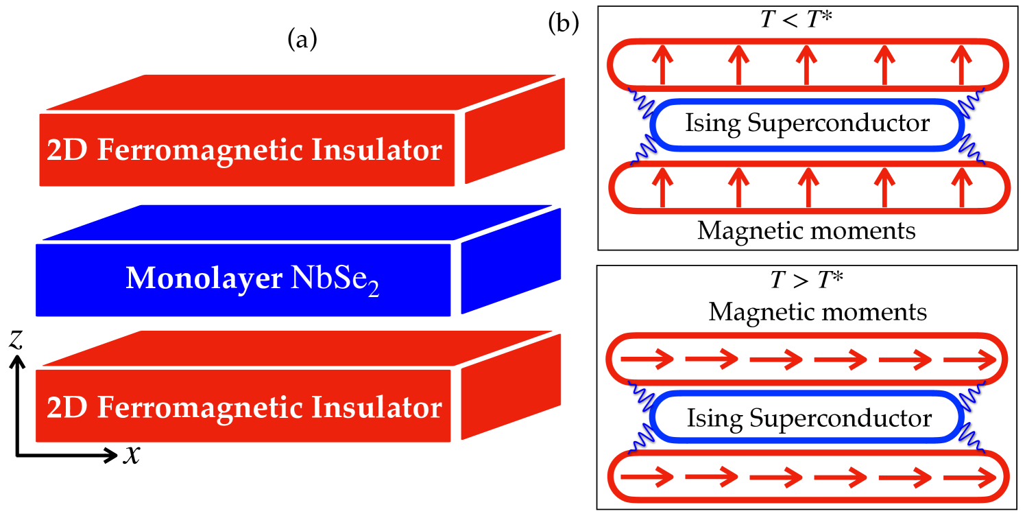
Here we put forward a magnet/superconductor van der Waals heterostructure as a controllable system where a magnetic transition is driven purely by Ising superconductivity. Specifically, we show that a monolayer-ferromagnet/NbSe₂/monolayer-ferromagnet [Fig. 1(a)] leads to an artificial system displaying magnetic transitions triggered by Ising superconductivity. We demonstrate how the interplay between the Ising superconductivity and the ferromagnetic proximity effect controls the magnetic alignment of the heterostructure. In particular, we show that the Ising SOC keeps the magnetic alignment of the heterostructure in-plane in the normal state, and drives a transition from in-plane to out-of-plane magnetic alignment in the superconducting state [Fig. 1(b)]. Our results put forward Ising superconductivity as a potential knob to control magnetism in artificial heterostructures, leading to a promising minimal building block for van-der-Waals-based superconducting spintronics.

The manuscript is organized as follows. First, in section II we present the effective model used to capture the physics of the ferromagnet/NbSe₂/ferromagnet heterostructures. In section III we discuss the interplay between Ising spin-orbit coupling, exchange coupling, and superconductivity. In section IV we show the emergence of magnetic switching driven by Ising superconductivity. Finally, in section V we summarize our results.

In the following we consider a multilayer structure consisting of a monolayer ${\rm{NbSe}}_{2}$ sandwiched between two ferromagnets, as shown in Fig. 1(a). The proximity effect between the ferromagnets and the superconducting layer induces an exchange field in the ${\rm{NbSe}}_{2}$. The direction of the induced field depends on the magnetization directions in the two ferromagnets. Overall, the net Hamiltonian of the system is

$$H=H_{0}+H_{SC}+H_{J},$$

(1)

where $H_{0}$ is the single-particle Hamiltonian of NbSe₂ including spin-orbit coupling, $H_{SC}$ accounts for the superconducting state and $H_{J}$ includes the effect of the ferromagnetic leads obtained by integrating out the CrI₃ degrees of freedom.

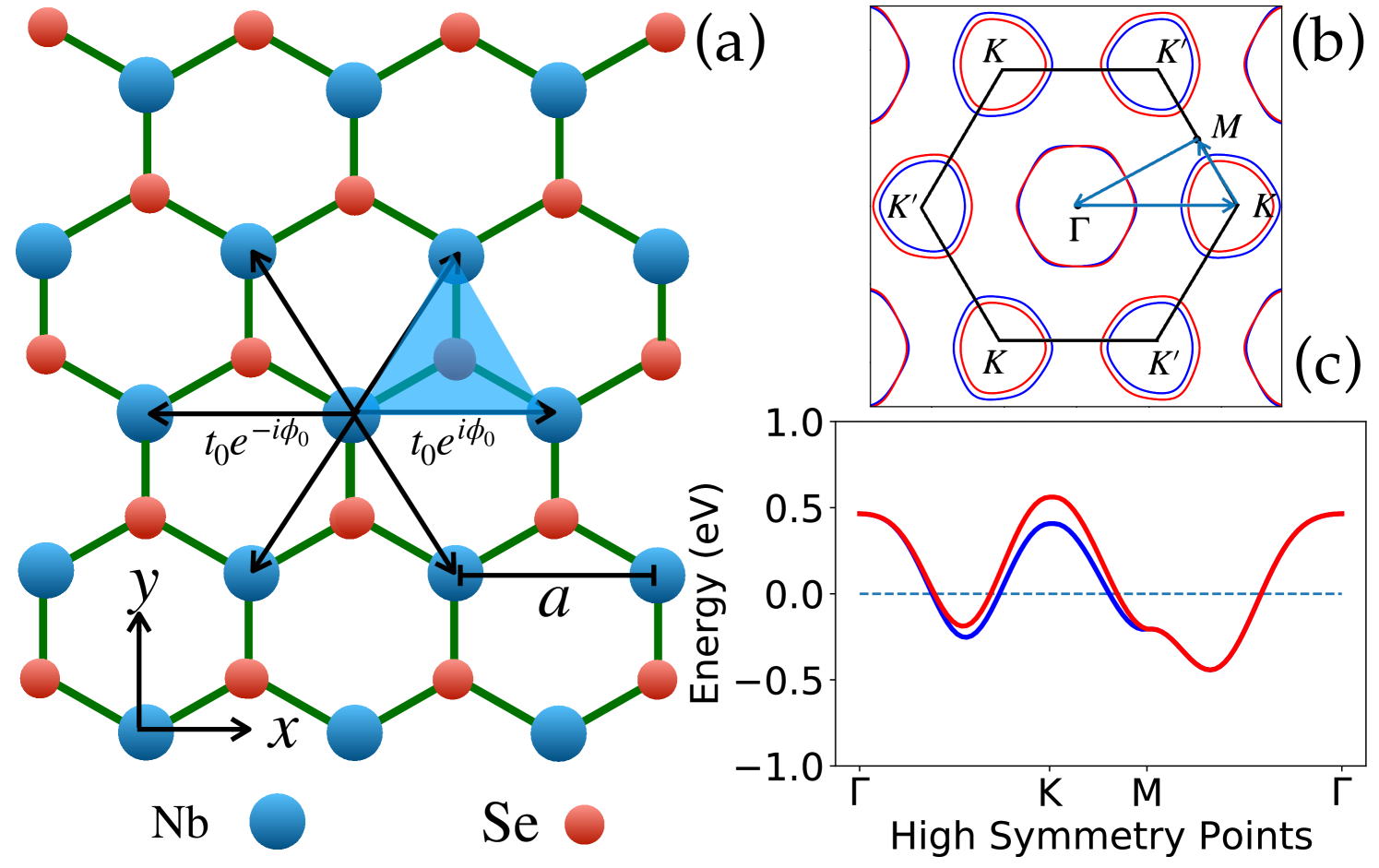
Let us first introduce the single-particle model $H_{0}$ for the ${\rm{NbSe}}_{2}$ layerFang et al. (2015); Liebhaber et al. (2019). To study the superconducting properties, only the low-energy part of the band structure is sufficient for consideration. The crystal structure of the monolayer $\rm{NbSe}_{2}$ has the $D_{3h}$ point-group symmetry, strongly constraining its lowest energy model. Since a single band is located at the Fermi energy Lebègue and Eriksson (2009), a Wannier Hamiltonian with a single orbital in the triangular lattice can be built [Fig. 2(a)]. The Wannier low energy model for NbSe₂ takes the form

$$H_{0}=\sum_{\alpha\beta}t^{ss^{\prime}}_{\alpha\beta}c^{\dagger}_{\alpha,s}c_{\beta,s^{\prime}},$$

(2)

where $t^{ss^{\prime}}_{\alpha\beta}$ are the spin-dependent hopping amplitudes¹¹1The values of the tight-binding parameters are given in appendix. A, and $c^{\dagger}_{i,s}$ is the creation operator of a Wannier orbital centered at each Nb site. This model captures the low-energy band structure of the monolayer $\rm{NbSe}_{2}$. The SOC is included by a Kane-Mele form Kane and Mele (2005) as a complex spin and bond dependent first neighbor complex hopping parameterized by a phase $\phi_{i}$. We include up the sixth neighbor hopping between Wannier orbitals. The resulting electronic structure is shown in Fig. 2(c).

The magnetic proximity effect with the top and bottom ferromagnets is included in the electronic structure of NbSe₂ as Khusainov (1996); Izyumov et al. (2002)

$$H_{J}=\sum_{k}\boldsymbol{J}\cdot\boldsymbol{\sigma}_{ss^{\prime}}c_{\boldsymbol{k}s}^{\dagger}c_{\boldsymbol{k}s^{\prime}}.$$

(3)

The superconducting term in the Hamiltonian is a conventional s-wave superconducting order of the form

$$H_{SC}=\sum_{\boldsymbol{k},\uparrow,\downarrow}\left(\Delta c_{\boldsymbol{k},\uparrow}^{\dagger}c_{-\boldsymbol{k},\downarrow}^{\dagger}+\Delta^{*}c_{-\boldsymbol{k},\downarrow}c_{\boldsymbol{k},\uparrow}\right)+K,$$

(4)

where $c_{\boldsymbol{k},s}^{(\dagger)}$ is the annihilation (creation) operator with spin $s$ at momentum $\boldsymbol{k}$, $\boldsymbol{\sigma}$ is the vector of Pauli spin matrices and $\boldsymbol{J}=(J_{x},J_{y},J_{z})$ is the vector of induced exchange field in the ${\rm{NbSe}_{2}}$ layers. It can be expressed in the spherical coordinates as $J_{x}=J\sin\theta\cos\varphi$, $J_{y}=J\sin\theta\sin\varphi$, and $J_{z}=J\cos\theta,$ where $J$ is the strength of the induced exchange field in the superconductor layer, and $\theta$ and $\varphi$ are the related polar and azimuthal angles, respectively.

The superconducting pair potential is determined self-consistently as $\Delta=g\int\left\langle c_{-\boldsymbol{k}\uparrow}c_{\boldsymbol{k}\downarrow}\right\rangle d^{2}\mathbf{k},$ where $g$ is the interaction potential. The last term in Eq. (4) then can be written as

$$K=g\int\left\langle c_{\boldsymbol{k}\uparrow}^{\dagger}c_{-\boldsymbol{k}\downarrow}^{\dagger}\right\rangle\Big{\langle}c_{-\boldsymbol{k}\downarrow}c_{\boldsymbol{k}\uparrow}\Big{\rangle}d^{2}\mathbf{k}=\frac{|\Delta|^{2}}{g}.$$

(5)

The contribution of superconductivity to the energetics of the system can be obtained by considering the free energy density. In general, the free energy density can be derived from the partition function Landau and Lifshitz (1980) $Z=e^{-K/k_{B}T}\prod_{\boldsymbol{k},n,\sigma}\left(1+e^{-\epsilon_{\boldsymbol{k},n,\sigma}/k_{B}T}\right)$, where $K$ is the constant term in the Hamiltonian in Eq. (4), $\epsilon_{\boldsymbol{k},n,\sigma}$ are the eigenvalues (with spin $\sigma$) of the Hamiltonian of the system under consideration, $T$ is the temperature and $k_{B}$ is the Boltzmann constant. We set $k_{B}=1$ hereafter. The band index $n$ runs only over the empty states. The free energy density is defined as $f=-T\log Z$. The detailed form of the free energy density can be written as

$$f=\frac{|\Delta|^{2}}{g}-T\sum_{\boldsymbol{k},n}\log\left[2+2\cosh\left(\frac{\epsilon_{\boldsymbol{k},n}}{T}\right)\right].$$

(6)

In the following, we concentrate on the free energy density $f_{s}$ of the superconducting state in the presence of exchange field compared to the free energy density $f_{n}$ in the normal state in the absence of the exchange field $f_{sn}=f_{s}({\bf J})-f_{n}(J=0)$.

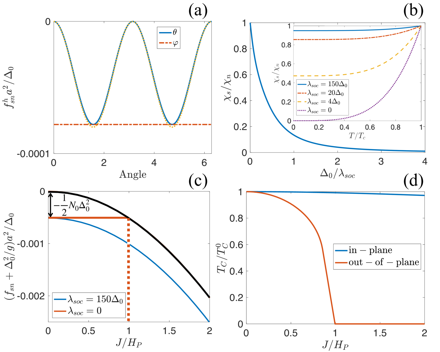
Before the discussion of the magnetic vdW heterostructure, it is instructive to summarize the properties of Ising superconductivity in the proximity of one ferromagnetic layer. The free energy density difference between the superconducting and normal state energy $f_{sn}$ has exchange field independent and dependent parts. The exchange field dependent part $f_{sn}^{h}=f_{sn}(\boldsymbol{J})-f_{sn}(\boldsymbol{J}=0)$ is plotted as a function of the angles of the exchange field in Fig. 3(a) for $T=0$. We can see that the superconductor energetically prefers an in-plane exchange field ($\theta=\pi/2$). This is a direct consequence of Ising superconductivity. For conventional superconductors, the free energy density $f_{sn}$ is the same for both in-plane and out-of-plane exchange fields below the Pauli paramagnetic limit. In superconductors with a lack of inversion symmetry (such as NbSe₂), the Ising spin-orbit interaction gives rise to a non-zero and anisotropic spin susceptibility even at $T=0$ Frigeri et al. (2004); Sigrist et al. (2009); Sohn et al. (2018).

The free energy density $f_{sn}$ of an Ising superconductor in the presence of an exchange field at $T=0$ can be written as²²2The definition of spin susceptibility and related derivations are given in appendix. C

$$f_{sn}=-\frac{1}{2}N(0)\Delta_{0}^{2}-\frac{1}{2}\chi_{s}(T=0)J^{2}\sin^{2}\theta,$$

(7)

where $N(0)$ is the density of states at the Fermi level, $\Delta_{0}$ is the superconducting pair potential at $T=0$ and $J=0$, and $\chi_{s}$ is the spin susceptibility for an in-plane exchange field describing the anisotropic spin response. For conventional superconductors, there is no such anisotropy, and the spin susceptibility vanishes at $T=0$ in the absence of spin relaxation. Yosida (1958).

The amount of anisotropy depends on the size of the spin-orbit coupling $\lambda_{\rm soc}$ so that for very large $\lambda_{\rm soc}$, the spin susceptibility $\chi_{s}$ for in-plane exchange field approaches the normal-state spin susceptibility. This is shown in Fig. 3(b) as a function of $\Delta_{0}/\lambda_{\rm soc}$ at $T=0$ and in the inset as a function of temperature. On the other hand, for an exchange field perpendicular to the plane, the spin susceptibility corresponds to the case with $\lambda_{\rm soc}=0$.

The anisotropic spin susceptibility in Ising superconductors also leads to an enhancement of the paramagetic critical field Bauer and Sigrist (2012); Youn et al. (2012). In the presence of an exchange field, the normal-state free energy density is lowered by the term $-\frac{1}{2}\chi_{n}(\theta)J^{2}$. When the exchange field breaks the superconducting order, $f_{sn}$ equals the paramagnetic energy density $f_{P}$ in the normal state

$$f_{P}=-\frac{1}{2}\chi_{n}(\theta)J^{2},$$

(8)

where $\chi_{n}(\theta)$ is the spin suceptibility in the normal state. Equating $f_{sn}$ and $f_{P}$ yields $J_{c}=\sqrt{\frac{N(0)}{\chi_{n}(\theta)-\chi_{s}(T=0)\sin^{2}\theta}}\Delta_{0}.$ Here $\chi_{n}(\theta)=\chi_{P}\cos^{2}\theta+\chi_{n}^{\rm soc}\sin^{2}\theta$, where $\chi_{P}=2N_{0}$ is the Pauli paramagnetic susceptibility, and $\chi_{n}^{\rm soc}$ is the normal state spin susceptibility caused by Ising SOC. For an out-of-plane field ($\theta=0$), the spin susceptibility is $\chi_{P}$ and the superconductivity experiences a first-order transition to the normal state, as shown in the red curve in Fig. 3(c). For $\theta=\pi/2$, the susceptibility is completely determined by $\chi_{n}^{\rm soc}$ and there is a second-order transition to the normal state at $J_{c}\gg H_{P}$. For the case of monolayer TMDs, $\chi_{n}^{\rm soc}\gg\chi_{P}$. For weak SOC, $\chi_{n}^{\rm soc}\rightarrow\chi_{P}$, and the normal state susceptibility is isotropic Frigeri et al. (2004). The critical temperature is also influenced by this anisotropic spin susceptibility. In Fig. 3(d), the critical temperature $T_{c}$ is shown for in- and out-of-plane exchange fields as a function of the exchange field strength $J$. One can see that $T_{c}$ remains nearly unchanged for increasing in-plane exchange field, but the superconductivity is destroyed at the Pauli paramagnetic limit for the out-of-plane exchange field.

The strength of the induced exchange field in the superconductor depends on many factors Izyumov et al. (2002); Bergeret et al. (2018); Bedoya-Pinto et al. (2021). If the induced exchange field is out-of-plane and is larger than the Pauli paramagnetic limit, $J>H_{P}$, the monolayer TMD remains in the normal state. However, the magnitude of $J$ depends on the chosen materials combination, and can also be below the critical field $H_{P}$. In what follows, we consider a case of the induced exchange field $J<H_{P}$ in the monolayer TMD Huang et al. (2017b); Bedoya-Pinto et al. (2021); Tartaglia et al. (2020a) so that it becomes superconducting at low enough temperature.

The direction of the exchange field is related to the magnetization direction of the ferromagnet, which is determined by the anisotropy energy. A monolayer ferromagnet such as ${\rm{CrI}_{3}}$ Huang et al. (2017c) and CrBr₃ Tartaglia et al. (2020a), shows a uniaxial anisotropy, and the anisotropy energy density can be written as

$$U_{{\rm{aniso}}}=K_{{\rm{eff}}}\sin^{2}\theta,$$

(9)

where $\theta$ is the polar angle of the magnetization direction with respect to the $z$ axis, and $K_{{\rm{eff}}}$ is the effective anisotropy constant with the unit of energy density. The main source of the effective anisotropy constant $K_{{\rm{eff}}}$ is the spin-orbit interactionLado and Fernández-Rossier (2017); Chen et al. (2020); Bacaksiz et al. (2021). The positive $K_{{\rm{eff}}}>0$ means the magnetization direction is along the easy-axis of the ferromagnet, and the negative $K_{{\rm{eff}}}<0$ would mean the magnetization direction is in the plane.

In the normal state, the anisotropic spin susceptibility caused by the spin-orbit interaction favors in-plane magnetic alignment, see Fig. 3(a). In the superconducting state, this tendency persists, but becomes weaker because the spin susceptibility is smaller in the superconducting state, as shown in Fig. 3(b). Then the direction of the exchange field in the Ising superconductor is determined by the competition of the anisotropy energy of the ferromagnet and the contribution of spin susceptibility to the free energy density of the superconductor. The part of total free energy density dependent on magnetization configuration can be written as

$$f_{{\rm{aniso}}}=\left(K_{\rm{eff}}-\frac{1}{2}\chi_{S}J^{2}\right)\sin^{2}\theta.$$

(10)

If the condition $K_{\rm{eff}}<\chi_{S}J^{2}/2$ holds, then the direction of the exchange field is in the plane. This relation is possible as the anisotropy energy of a monolayer ferromagnet can be tuned by various means. For example, the magnetic anisotropy can be engineered by strain Webster and Yan (2018) and by controlling the SOC via chemical tuning Tartaglia et al. (2020a). In other words, the anisotropic spin susceptibility leads to the switching of an off-plane easy axis anisotropy to the easy plane anisotropy if $K_{\rm{eff}}<\chi_{S}J^{2}/2$. With this mechanism in mind, let us now discuss how the interplay between superconductivity driven-magnetic switching would affect the coupling between two ferromagnets.

In the following, we consider a Ferromagnet/Superconductor/Ferromagnet (F/S/F) structure, in which the easy axis of the ferromagnets is influenced by the presence of superconductivity. The magnetic moments in the ferromagnets are coupled through the superconducting layer, and this coupling also determines the direction of the induced exchange field. The full energetics of the system can be written as

$$f_{{\rm{aniso}}}=K_{1}\sin^{2}\theta_{1}+K_{2}\sin^{2}\theta_{2}+\delta f_{sn},$$

(11)

where $K_{1/2}$ are the effective anisotropy constants of the two ferromagnets, $\theta_{1/2}$ are the related polar angles, and $\delta f_{sn}$ is the contribution of superconductivity to the anisotropy energy density.

It is first worth noting how this mechanism would work in a conventional superconductor. For a conventional superconductor with thickness smaller than the superconducting coherence length, the coupling between the ferromagnets through the superconducting layer gives rise to an antiparallel configuration of the magnetization directions Gennes (1966); Hauser (1969); Ojajärvi et al. (2021). The contribution of this coupling to the energetics of the system $\delta f_{sn}$ is evaluated as $\delta f_{sn}=N(0)\bar{J}^{2}\cos^{2}\left[\frac{1}{2}\left(\theta_{1}-\theta_{2}\right)\right],$ where $\bar{J}$ would be the strength of the induced exchange field in the metallic film. Because of this term, the antiparallel alignment of the magnetization directions is favoured in the system. However, and in stark contrast, for the case of a vdW heterostructure containing a two-dimensional Ising superconductor, the ferromagnetic layers couple through the spin susceptibility ³³3Direct coupling mediated by NbSe₂ is stronger than indirect superexchange between layers. We now write the components of the exchange field as $J_{x}=J(\sin\theta_{1}\cos\psi_{1}+\sin\theta_{2}\cos\psi_{2})$, $J_{y}=J(\sin\theta_{1}\sin\psi_{1}+\sin\theta_{2}\sin\psi_{2})$, $J_{z}=J(\cos\theta_{1}+\cos\theta_{2})$ in the Hamiltonian in Eq. (3), diagonalize the Hamiltonian in Eq. (1), obtaining the contribution of this coupling to the energetics of the system $\delta f_{sn}=-\frac{1}{2}\chi_{s}J^{2}\left(\sin\theta_{1}+\sin\theta_{2}\right)^{2}.$ The overall effect of this term is to lower the total anisotropy energy. Hence a parallel alignment maximizes this effect. This is opposite to the case of a thin metallic superconductor discussed above, where an antiparallel alignment is energetically favoured. Note that, our discussion above neglects direct Heisenberg coupling between the magnetic monolayers. The nature of that coupling can be ferromagnetic or antiferromagnetic depending on the geometric details. A well known example is the case of CrI₃ bilayersHuang et al. (2017d); Soriano et al. (2019); Sivadas et al. (2018); Ubrig et al. (2019), where depending on the relative alignment between layers the coupling can be either ferromagnetic or antiferromagnetic. This contribution is a higher order superexchange depending on the valence states of each element, can be only captured properly with quantum chemistry density functional theory calculations and can potentially depend on the geometric alignment between monolayersHuang et al. (2017d); Soriano et al. (2019); Sivadas et al. (2018); Ubrig et al. (2019). This contribution would determine the relative orientation of the magnetization between the two magnetic monolayers, and for the sake of concreteness in Fig. 1 was taken as ferromagnetic.

The ferromagnetic coupling mediated by Ising superconductivity can be detected by a magnetic hysteresis measurement. We use the Stoner–Wohlfarth (SW) model Stoner and Wohlfarth (1948); Tannous and Gieraltowski (2008) to calculate the hysteresis loop. In the SW model, the directions of the magnetization density $M$ and the external applied field $H$ are characterized by different angles with respect to the easy axis (polar angles). In the system we are considering, there is also the contribution of the superconductor to the anisotropy energy. Then the magnetization density is subjected to the competition between the anisotropy energy and Zeeman energy caused by the external applied field. The total anisotropy energy density is written as

$$\begin{split}&f_{{\rm{aniso}}}=K_{1}\sin^{2}\theta_{1}+K_{2}\sin^{2}\theta_{2}+\delta f_{sn}\\ &-HM_{s1}\cos\left(\theta_{1}-\vartheta\right)-HM_{s2}\cos\left(\theta_{2}-\vartheta\right),\end{split}$$

(12)

where $H$ is the external applied field, $M_{s1/2}$ is the saturation magnetization density in the two ferromagnets, and $\vartheta$ is the angle between the easy axis and the direction of the external magnetic field. Substituting the value of $\delta f_{sn}$, we have

$$\begin{split}f_{{\rm{aniso}}}&=\left(K_{1}-\frac{1}{2}\chi_{s}J^{2}\right)\sin^{2}\theta_{1}\\ &+\left(K_{2}-\frac{1}{2}\chi_{s}J^{2}\right)\sin^{2}\theta_{2}-\chi_{s}J^{2}\sin\theta_{1}\sin\theta_{2}\\ &-HM_{s1}\cos\left(\theta_{1}-\vartheta\right)-HM_{s2}\cos\left(\theta_{2}-\vartheta\right).\end{split}$$

(13)

The hysteresis curve is then obtained by calculating the longitudinal and transverse components of the magnetization density

$$M_{z}=M_{s1}\cos\theta_{1}^{*}+M_{s2}\cos\theta_{2}^{*},$$

(14)

$$M_{x}=M_{s1}\sin\theta_{1}^{*}+M_{s2}\sin\theta_{2}^{*},$$

(15)

where $\theta_{1/2}^{*}$ are the angles for which the total anisotropy energy density $f_{{\rm{aniso}}}$ is minimized.

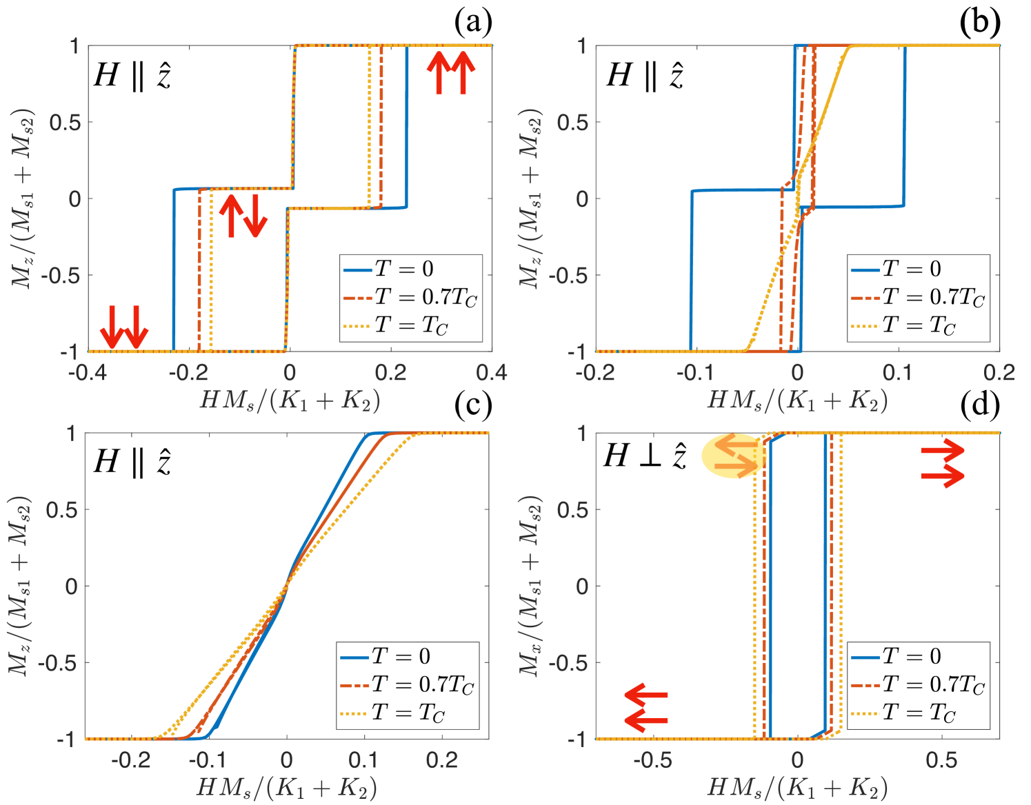
For an easy axis ferromagnet such as CrBr₃ or CrI₃, the induced exchange field is out-of-plane. In the absence of the Ising superconductor, the magnetic alignment of the system is ferromagnetic and two coercive fields appear in the hysteresis curve at $H_{c1}M_{s}=\pm 2K_{1}$ and $H_{c2}M_{s}=\pm 2K_{2}$. If the anisotropy energy of the ferromagnet is larger than the contribution $\delta f_{sn}$ of the superconductor, the net effect of the Ising superconductor leads to a modification of the anisotropy constants, as can be seen from Eq. (13). The modification shifts the coercive fields as $H_{c1}M_{s}=\pm 2(K_{1}-\chi_{s}J^{2})$ and $H_{c2}M_{s}=\pm 2(K_{2}-\chi_{s}J^{2})$. We can see that, if the values of $K_{1}$ and $K_{2}$ are comparable with $\chi_{s}J^{2}$, the temperature dependence of the anisotropic spin susceptibility causes significant modifications to the hysteresis curves. In order to see such modifications, the difference between $K_{1}$ and $K_{2}$ must be smaller than the difference of the spin susceptibility $\chi_{s}$ at $T_{c}$ and $T=0$. In the following calculations, we set $\lambda_{\rm soc}=150\Delta_{0}$, $K_{1}=1.12K_{2}$ and $M_{s1}=1.12M_{s2}=1.12M_{s}$ to illustrate how superconductivity affects the magnetic hysteresis in a temperature dependent manner. The hysteresis curve is shown in Fig. 4. It is worth noting that, while $\lambda_{\rm soc}/\Delta$ cannot be efficiently tuned in a specific material, specific ratios can be obtained by taking different dichalcogenides including 1H-TaS₂, 1H-TaSe₂, 1H-NbS₂, 1H-NbSe₂, and potentially continuously using dichalcogenide alloysZhao et al. (2019).

The modified coercive fields for strong anisotropy fields $K_{i}>\chi_{s}J^{2}$ are shown in the hysteresis curve in Fig. 4(a). Decreasing the temperature, $\chi_{s}$ becomes smaller, and the difference in the coercive fields becomes larger. In the opposite case $K_{i}<\chi_{s}J^{2}$, the induced field is in the plane, and there is no hysteresis for an out-of-plane component of the magnetization density $M_{z}$, as shown in Fig. 4(c). The hysteresis curve for $M_{x}$ is shown in Fig. 4(d). Contrary to the case in Fig. 4(a), the location of the coercive fields moves closer at lower temperature for smaller $\chi_{s}$.

A more interesting case takes place for ferromagnets with anisotropy constants with intermediate valuesTartaglia et al. (2020b). In this case, the induced exchange field is out-of-plane at low temperature and in-plane at a higher temperature. This transition takes place at a temperature $T=T^{*}$ and is due to the temperature dependence of the spin susceptibility $\chi_{s}$, so that the induced field is in-plane for a temperature $T>T^{*}$. This case is shown in Fig. 4(b). In this limit, an in-plane exchange field is favoured in Ising superconducting and normal states for $T>T^{*}$. Note that, besides moving the coercive fields of single magnets, NbSe₂ promotes a ferromagnetic coupling between the magnets in the normal state. This affects the hysteresis curves by reducing the region with antiparallel magnetization directions, but cannot be directly measured in situ because of a lack of a control measurement without the presence of NbSe₂. In the superconducting state this ferromagnetic coupling decreases but, unlike the coupling mediated by a conventional superconductor, does not become antiferromagnetic.

It is also worth noting that, beyond the NbSe₂ platform considered here, this phenomenology can also potentially take place for generic monolayer Ising superconductors, for example electron doped MoS₂ Lu et al. (2015); Costanzo et al. (2016) and other TMD monolayers like TaS₂/TaSe₂ Li et al. (2020). For other potential candidates with smaller spin-orbit coupling, the dependence of the anisotropic spin susceptibility on temperature is stronger, see Fig. 3(b). Then the hysteresis curves can be obtained for more varied anisotropy fields.

Interestingly, while magnetic order is often controlled by external knobs such as magnetic field, here we propose a radically different mechanism in which the magnetic order itself is controlled by the superconducting order in one of the components of the heterostructure. These results highlight that Ising superconductivity controls the way how the system reacts to magnetic fields, an effect that can be present in a variety of superconductor-ferromagnet van der Waals heterostructures. From the practical point of view, we exploit the unique temperature dependence of $\chi_{s}$, to uncover the interplay between the magnetism and superconductivity.

Besides magnetic hysteresis that in 2D materials can be measured with the magneto-optical Kerr effect, the anisotropic spin susceptibility of the Ising superconductivity can be accessed also via the ferromagnetic resonance of the multilayer system.Ojajärvi et al. (2021)

For the possible experimental realization, below we briefly elaborate on the most promising materials candidates based on recent experiments. First, recent experiments demonstrated heterostructures of the monolayer ferromagnet with CrBr₃ on bulk NbSe₂ Kezilebieke et al. (2020), making CrBr₃ a promising candidate for our proposal. While the experiment focused on a monolayer CrBr₃ on top of a bulk NbSe₂, it is worth noting that the value of the exchange proximity would be comparable for a monolayer NbSe₂ given its van der Waals nature. From the point of view of the ferromagnetic insulator candidates, apart from CrBr₃, CrI₃ Huang et al. (2017b), CrCl₃ Bedoya-Pinto et al. (2021) and recently synthetised chromium heterohalides Tartaglia et al. (2020a) would provide excellent candidates. Importantly, van der Waals chromium heterohalides have been demonstrated to have a completely tunable magnetic anisotropy, making them outstanding candidates for our proposal Tartaglia et al. (2020a). Finally, we note that the magnetic anisotropy could also be engineered by strain Webster and Yan (2018), yet this approach could be more challenging from the experimental point of view.

It is finally worth mentioning that the possible moiré patterns between the layers Tong et al. (2019); Wang et al. (2020) and correlation effects Huang et al. (2016); Wang et al. (2020) in the TMDs have an influence on the effective values of the parameters used in our model. These effects modify the band structure of the middle layer, especially the splitting around the K points. However, the correlation effects in the ferromagnetic layers, for example magnetic excitations Chen et al. (2018); Costa et al. (2020); Jin et al. (2018) do not directly influence the results, as these effects do not modify the form of the low energy Hamiltonian for the hybrid heterostructure we are considering.

To summarize, we demonstrate how Ising superconductivity allows controlling the magnetic coupling in ferromagnet/NbSe₂/ferromagnet heterostructures. In particular, we show that the anisotropic spin response inherited by the Ising superconductor allows flipping the magnetic alignment upon entering the superconducting state. We show that the contribution of the Ising superconductivity to the energetics of the system stems from an anisotropic spin susceptibility. In the magnetic vdW heterostructure, the coupling between the ferromagnets is achieved through the anisotropic spin susceptibility, which gives rise to a parallel alignment of the magnetization directions, both in the superconducting and normal states. Interestingly, such magnetic switching was shown to lead to a hysteretic behavior in the magnetic alignment purely driven by the spin susceptibility of the NbSe₂ inherited from Ising spin-orbit coupling. Our results put forward superconductor/ferromagnet van der Waals heterostructures as a novel platform to explore superconducting spintronics phenomena dominated by Ising spin-orbit coupling effects.

Acknowledgments: We acknowledge the computational resources provided by the Aalto Science-IT project, and the financial support from the Academy of Finland Projects No. 331342, No. 336243 and No. 317118, and the Jane and Aatos Erkko Foundation.

References

- Novoselov et al. (2016) K. S. Novoselov, A. Mishchenko, A. Carvalho, and A. H. C. Neto, Science 353, aac9439 (2016).
- Geim and Grigorieva (2013) A. K. Geim and I. V. Grigorieva, Nature 499, 419 (2013).
- Liu et al. (2016) Y. Liu, N. O. Weiss, X. Duan, H.-C. Cheng, Y. Huang, and X. Duan, Nature Rev. Mat. 1, 10.1038/natrevmats.2016.42 (2016).
- Neto (2001) A. H. C. Neto, Phys. Rev. Lett. 86, 4382 (2001).
- Saito et al. (2016) Y. Saito, T. Nojima, and Y. Iwasa, Nature Rev. Mat. 2, 10.1038/natrevmats.2016.94 (2016).
- Qiu et al. (2021) D. Qiu, C. Gong, S. Wang, M. Zhang, C. Yang, X. Wang, and J. Xiong, Advanced Materials 33, 2006124 (2021).
- Shabbir et al. (2018) B. Shabbir, M. Nadeem, Z. Dai, M. S. Fuhrer, Q.-K. Xue, X. Wang, and Q. Bao, Applied Physics Reviews 5, 041105 (2018).
- Gong et al. (2017) C. Gong, L. Li, Z. Li, H. Ji, A. Stern, Y. Xia, T. Cao, W. Bao, C. Wang, Y. Wang, Z. Q. Qiu, R. J. Cava, S. G. Louie, J. Xia, and X. Zhang, Nature 546, 265 (2017).
- Huang et al. (2017a) B. Huang, G. Clark, E. Navarro-Moratalla, D. R. Klein, R. Cheng, K. L. Seyler, D. Zhong, E. Schmidgall, M. A. McGuire, D. H. Cobden, W. Yao, D. Xiao, P. Jarillo-Herrero, and X. Xu, Nature 546, 270 (2017a).
- Zhang et al. (2019) Z. Zhang, J. Shang, C. Jiang, A. Rasmita, W. Gao, and T. Yu, Nano Lett. 19, 3138 (2019).
- Ghazaryan et al. (2018) D. Ghazaryan, M. T. Greenaway, Z. Wang, V. H. Guarochico-Moreira, I. J. Vera-Marun, J. Yin, Y. Liao, S. V. Morozov, O. Kristanovski, A. I. Lichtenstein, M. I. Katsnelson, F. Withers, A. Mishchenko, L. Eaves, A. K. Geim, K. S. Novoselov, and A. Misra, Nature Electronics 1, 344 (2018).
- Kezilebieke et al. (2020) S. Kezilebieke, M. N. Huda, V. Vaňo, M. Aapro, S. C. Ganguli, O. J. Silveira, S. Głodzik, A. S. Foster, T. Ojanen, and P. Liljeroth, Nature 588, 424 (2020).
- Kezilebieke et al. (2021) S. Kezilebieke, O. J. Silveira, M. N. Huda, V. Vaňo, M. Aapro, S. C. Ganguli, J. Lahtinen, R. Mansell, S. Dijken, A. S. Foster, and P. Liljeroth, Advanced Materials 33, 2006850 (2021).
- Kang et al. (2021) K. Kang, S. Jiang, H. Berger, K. Watanabe, T. Taniguchi, L. Forró, J. Shan, and K. F. Mak, arXiv e-prints , arXiv:2101.01327 (2021), arXiv:2101.01327 [cond-mat.supr-con] .
- Kezilebieke et al. (2020) S. Kezilebieke, V. Vaňo, M. N. Huda, M. Aapro, S. C. Ganguli, P. Liljeroth, and J. L. Lado, arXiv e-prints , arXiv:2011.09760 (2020), arXiv:2011.09760 [cond-mat.mes-hall] .
- Manzeli et al. (2017) S. Manzeli, D. Ovchinnikov, D. Pasquier, O. V. Yazyev, and A. Kis, Nature Rev. Mat. 2, 10.1038/natrevmats.2017.33 (2017).
- Zhu et al. (2011) Z. Y. Zhu, Y. C. Cheng, and U. Schwingenschlögl, Phys. Rev. B 84, 10.1103/physrevb.84.153402 (2011).
- Xiao et al. (2012) D. Xiao, G.-B. Liu, W. Feng, X. Xu, and W. Yao, Phys. Rev. Lett. 108, 10.1103/physrevlett.108.196802 (2012).
- Kormányos et al. (2014) A. Kormányos, V. Zólyomi, N. D. Drummond, and G. Burkard, Physical Review X 4, 10.1103/physrevx.4.011034 (2014).
- Soriano and Lado (2020) D. Soriano and J. L. Lado, Journal of Physics D: Applied Physics 53, 474001 (2020).
- Cortés et al. (2019) N. Cortés, O. Ávalos-Ovando, L. Rosales, P. A. Orellana, and S. E. Ulloa, Phys. Rev. Lett. 122, 086401 (2019).
- Henriques et al. (2020) J. C. G. Henriques, G. Catarina, A. T. Costa, J. Fernández-Rossier, and N. M. R. Peres, Phys. Rev. B 101, 045408 (2020).
- Zollner et al. (2019) K. Zollner, P. E. Faria Junior, and J. Fabian, Phys. Rev. B 100, 085128 (2019).
- Xu et al. (2014) X. Xu, W. Yao, D. Xiao, and T. F. Heinz, Nature Physics 10, 343 (2014).
- Xi et al. (2015) X. Xi, Z. Wang, W. Zhao, J.-H. Park, K. T. Law, H. Berger, L. Forró, J. Shan, and K. F. Mak, Nature Physics 12, 139 (2015).
- Lu et al. (2015) J. M. Lu, O. Zheliuk, I. Leermakers, N. F. Q. Yuan, U. Zeitler, K. T. Law, and J. T. Ye, Science 350, 1353 (2015).
- Saito et al. (2015) Y. Saito, Y. Nakamura, M. S. Bahramy, Y. Kohama, J. Ye, Y. Kasahara, Y. Nakagawa, M. Onga, M. Tokunaga, T. Nojima, Y. Yanase, and Y. Iwasa, Nature Physics 12, 144 (2015).
- Youn et al. (2012) S. J. Youn, M. H. Fischer, S. H. Rhim, M. Sigrist, and D. F. Agterberg, Phys. Rev. B 85, 10.1103/physrevb.85.220505 (2012).
- de la Barrera et al. (2018) S. C. de la Barrera, M. R. Sinko, D. P. Gopalan, N. Sivadas, K. L. Seyler, K. Watanabe, T. Taniguchi, A. W. Tsen, X. Xu, D. Xiao, and B. M. Hunt, Nature Communications 9, 10.1038/s41467-018-03888-4 (2018).
- Rahimi et al. (2017) M. A. Rahimi, A. G. Moghaddam, C. Dykstra, M. Governale, and U. Zülicke, Physical Review B 95, 104515 (2017).
- Fang et al. (2015) S. Fang, R. Kuate Defo, S. N. Shirodkar, S. Lieu, G. A. Tritsaris, and E. Kaxiras, Phys. Rev. B 92, 205108 (2015).
- Liebhaber et al. (2019) E. Liebhaber, S. A. González, R. Baba, G. Reecht, B. W. Heinrich, S. Rohlf, K. Rossnagel, F. von Oppen, and K. J. Franke, Nano Lett. 20, 339 (2019).
- Lebègue and Eriksson (2009) S. Lebègue and O. Eriksson, Phys. Rev. B 79, 10.1103/physrevb.79.115409 (2009).
- Note (1) The values of the tight-binding parameters are given in appendix. A.
- Kane and Mele (2005) C. L. Kane and E. J. Mele, Phys. Rev. Lett. 95, 10.1103/physrevlett.95.226801 (2005).
- Khusainov (1996) M. G. Khusainov, Eksp. Teor. Fiz. 109, 524 (1996).
- Izyumov et al. (2002) Y. A. Izyumov, Y. N. Proshin, and M. G. Khusainov, Uspekhi Fizicheskikh Nauk (UFN) Journal 45, 109 (2002).
- Landau and Lifshitz (1980) L. D. Landau and E. M. Lifshitz, eds., Statistical Physics (Elsevier, 1980).
- Frigeri et al. (2004) P. A. Frigeri, D. F. Agterberg, and M. Sigrist, New Journal of Physics 6, 115 (2004).
- Sigrist et al. (2009) M. Sigrist, A. Avella, and F. Mancini, in AIP Conference Proceedings (AIP, 2009).
- Sohn et al. (2018) E. Sohn, X. Xi, W.-Y. He, S. Jiang, Z. Wang, K. Kang, J.-H. Park, H. Berger, L. Forró, K. T. Law, J. Shan, and K. F. Mak, Nature Materials 17, 504 (2018).
- Note (2) The definition of spin susceptibility and related derivations are given in appendix. C.
- Yosida (1958) K. Yosida, Phys. Rev. 110, 769 (1958).
- Bauer and Sigrist (2012) E. Bauer and M. Sigrist, eds., Non-Centrosymmetric Superconductors (Springer Berlin Heidelberg, 2012).
- Bergeret et al. (2018) F. S. Bergeret, M. Silaev, P. Virtanen, and T. T. Heikkilä, Rev. Mod. Phys. 90, 041001 (2018).
- Bedoya-Pinto et al. (2021) A. Bedoya-Pinto, J.-R. Ji, A. K. Pandeya, P. Gargiani, M. Valvidares, P. Sessi, J. M. Taylor, F. Radu, K. Chang, and S. S. P. Parkin, Science 374, 616–620 (2021).
- Huang et al. (2017b) B. Huang, G. Clark, E. Navarro-Moratalla, D. R. Klein, R. Cheng, K. L. Seyler, D. Zhong, E. Schmidgall, M. A. McGuire, D. H. Cobden, and et al., Nature 546, 270–273 (2017b).
- Tartaglia et al. (2020a) T. A. Tartaglia, J. N. Tang, J. L. Lado, F. Bahrami, M. Abramchuk, G. T. McCandless, M. C. Doyle, K. S. Burch, Y. Ran, J. Y. Chan, and F. Tafti, Science Advances 6, eabb9379 (2020a).
- Huang et al. (2017c) B. Huang, G. Clark, E. Navarro-Moratalla, D. R. Klein, R. Cheng, K. L. Seyler, D. Zhong, E. Schmidgall, M. A. McGuire, D. H. Cobden, W. Yao, D. Xiao, P. Jarillo-Herrero, and X. Xu, Nature 546, 270 (2017c).
- Lado and Fernández-Rossier (2017) J. L. Lado and J. Fernández-Rossier, 2D Materials 4, 035002 (2017).
- Chen et al. (2020) L. Chen, J.-H. Chung, T. Chen, C. Duan, A. Schneidewind, I. Radelytskyi, D. J. Voneshen, R. A. Ewings, M. B. Stone, A. I. Kolesnikov, B. Winn, S. Chi, R. A. Mole, D. H. Yu, B. Gao, and P. Dai, Phys. Rev. B 101, 10.1103/physrevb.101.134418 (2020).
- Bacaksiz et al. (2021) C. Bacaksiz, D. Šabani, R. M. Menezes, and M. V. Milošević, Phys. Rev. B 103, 10.1103/physrevb.103.125418 (2021).
- Webster and Yan (2018) L. Webster and J.-A. Yan, Phys. Rev. B 98, 144411 (2018).
- Gennes (1966) P. D. Gennes, Physics Letters 23, 10 (1966).
- Hauser (1969) J. J. Hauser, Phys. Rev. Lett. 23, 374 (1969).
- Ojajärvi et al. (2021) R. Ojajärvi, F. Bergeret, M. Silaev, and T. T. Heikkilä, arXiv:2107.09959 (2021).
- Note (3) Direct coupling mediated by NbSe2 is stronger than indirect superexchange between layers.
- Huang et al. (2017d) B. Huang, G. Clark, E. Navarro-Moratalla, D. R. Klein, R. Cheng, K. L. Seyler, D. Zhong, E. Schmidgall, M. A. McGuire, D. H. Cobden, W. Yao, D. Xiao, P. Jarillo-Herrero, and X. Xu, Nature 546, 270 (2017d).
- Soriano et al. (2019) D. Soriano, C. Cardoso, and J. Fernández-Rossier, Solid State Communications 299, 113662 (2019).
- Sivadas et al. (2018) N. Sivadas, S. Okamoto, X. Xu, C. J. Fennie, and D. Xiao, Nano Letters 18, 7658 (2018).
- Ubrig et al. (2019) N. Ubrig, Z. Wang, J. Teyssier, T. Taniguchi, K. Watanabe, E. Giannini, A. F. Morpurgo, and M. Gibertini, 2D Materials 7, 015007 (2019).
- Stoner and Wohlfarth (1948) E. C. Stoner and E. P. Wohlfarth, Philosophical Transactions of the Royal Society of London. Series A, Mathematical and Physical Sciences 240, 599 (1948).
- Tannous and Gieraltowski (2008) C. Tannous and J. Gieraltowski, European Journal of Physics 29, 475 (2008).
- Zhao et al. (2019) K. Zhao, H. Lin, X. Xiao, W. Huang, W. Yao, M. Yan, Y. Xing, Q. Zhang, Z.-X. Li, S. Hoshino, J. Wang, S. Zhou, L. Gu, M. S. Bahramy, H. Yao, N. Nagaosa, Q.-K. Xue, K. T. Law, X. Chen, and S.-H. Ji, Nature Physics 15, 904 (2019).
- Tartaglia et al. (2020b) T. A. Tartaglia, J. N. Tang, J. L. Lado, F. Bahrami, M. Abramchuk, G. T. McCandless, M. C. Doyle, K. S. Burch, Y. Ran, J. Y. Chan, and F. Tafti, Science Advances 6, eabb9379 (2020b).
- Costanzo et al. (2016) D. Costanzo, S. Jo, H. Berger, and A. F. Morpurgo, Nature nanotechnology 11, 339 (2016).
- Li et al. (2020) J. Li, P. Song, J. Zhao, K. Vaklinova, X. Zhao, Z. Li, Z. Qiu, Z. Wang, L. Lin, M. Zhao, T. S. Herng, Y. Zuo, W. Jonhson, W. Yu, X. Hai, P. Lyu, H. Xu, H. Yang, C. Chen, S. J. Pennycook, J. Ding, J. Teng, A. H. C. Neto, K. S. Novoselov, and J. Lu, Nature Materials 20, 181 (2020).
- Tong et al. (2019) Q. Tong, M. Chen, and W. Yao, Phys. Rev. Applied 12, 024031 (2019).
- Wang et al. (2020) L. Wang, E.-M. Shih, A. Ghiotto, L. Xian, D. A. Rhodes, C. Tan, M. Claassen, D. M. Kennes, Y. Bai, B. Kim, et al., Nature materials 19, 861 (2020).
- Huang et al. (2016) P.-R. Huang, Q.-Y. Chen, H. K. Pal, M. Kindermann, C. Cao, and Y. He, Superlattices and Microstructures 100, 997 (2016).
- Chen et al. (2018) L. Chen, J.-H. Chung, B. Gao, T. Chen, M. B. Stone, A. I. Kolesnikov, Q. Huang, and P. Dai, Phys. Rev. X 8, 041028 (2018).
- Costa et al. (2020) A. T. Costa, D. L. R. Santos, N. M. Peres, and J. Fernández-Rossier, 2D Materials 7, 045031 (2020).
- Jin et al. (2018) W. Jin, H. H. Kim, Z. Ye, S. Li, P. Rezaie, F. Diaz, S. Siddiq, E. Wauer, B. Yang, C. Li, et al., Nature communications 9, 1 (2018).
- He et al. (2018) W.-Y. He, B. T. Zhou, J. J. He, N. F. Q. Yuan, T. Zhang, and K. T. Law, Communications Physics 1, 10.1038/s42005-018-0041-4 (2018).
- Zheng et al. (2018) F. Zheng, Z. Zhou, X. Liu, and J. Feng, Phys. Rev. B 97, 081101 (2018).
- Gor'kov and Rashba (2001) L. P. Gor'kov and E. I. Rashba, Phys. Rev. Lett. 87, 10.1103/physrevlett.87.037004 (2001).