Convectively stabilised background solar models for local helioseismology

One of the goals of local helioseismology is to interpret observations of the solar oscillations in the vicinity of sunspots and active regions. Kilogauss magnetic fields near the surface of the Sun have a strong effect on solar oscillations, which cannot be computed easily using perturbation theory. Numerical simulations of wave propagation may be the only realistic way to model these effects accurately. Two approaches have been proposed. The first one is to solve the equations of radiative MHD (e.g. Rempel et al. 2009) in order to model the magnetic structures and the (naturally excited) seismic waves simultaneously. The second approach is to compute the propagation of waves through a prescribed magnetised background model (e.g. Cally & Bogdan 1997, Cameron et al. 2007, 2008). While the first approach is more realistic, the second approach is less computer intensive.

Here, as a first step, we consider the problem of simulating the time evolution of small-amplitude waves through a quiet Sun background atmosphere using the Semi-spectral Linear MHD code (Cameron et al. 2007). In principle, any realistic model of the upper layers of the Sun, such as Model S (Christensen-Dalsgaard et al. 1996), is convectively unstable. It is however not possible to use Model S as a background model for an initial-value linear-wave calculation, since the convective modes will grow exponentially and quickly dominate the solution. These convective modes must be dealt with.

We impose two main conditions for constructing a quiet-Sun model, which can be used in our simulations: (C1) it must be convectively stable and (C2) it must support oscillations which have solar-like eigenfrequencies and eigenfunctions.We choose to begin from Model S and to modify it so that the resulting model best satisfies these conditions.

There are various ways to achieve convective stability. For example, one may adjust the adiabatic exponent of the model. In this study, we choose to increase slightly the pressure gradient such that $\partial_{z}p>c^{2}\partial_{z}\rho$, where the sound speed, $c$, and the density gradient, $\partial_{z}\rho$, are retained from Model S. This guarantees that condition (C1) is met. The drawback is that the p-mode kinetic energy densities are too small near the surface compared to those of Model S and that the frequencies of the p modes are slightly too high. We can compensate for this by changing the sound speed by a few per cent near the surface (details and justification discussed by Schunker et al. (in preparation). We arrive at a particular Convectively Stabilised Model (CSM), which has eigenfunctions that are as close as possible to Model S while the eigenfrequencies remain within about 2% of Model S values.

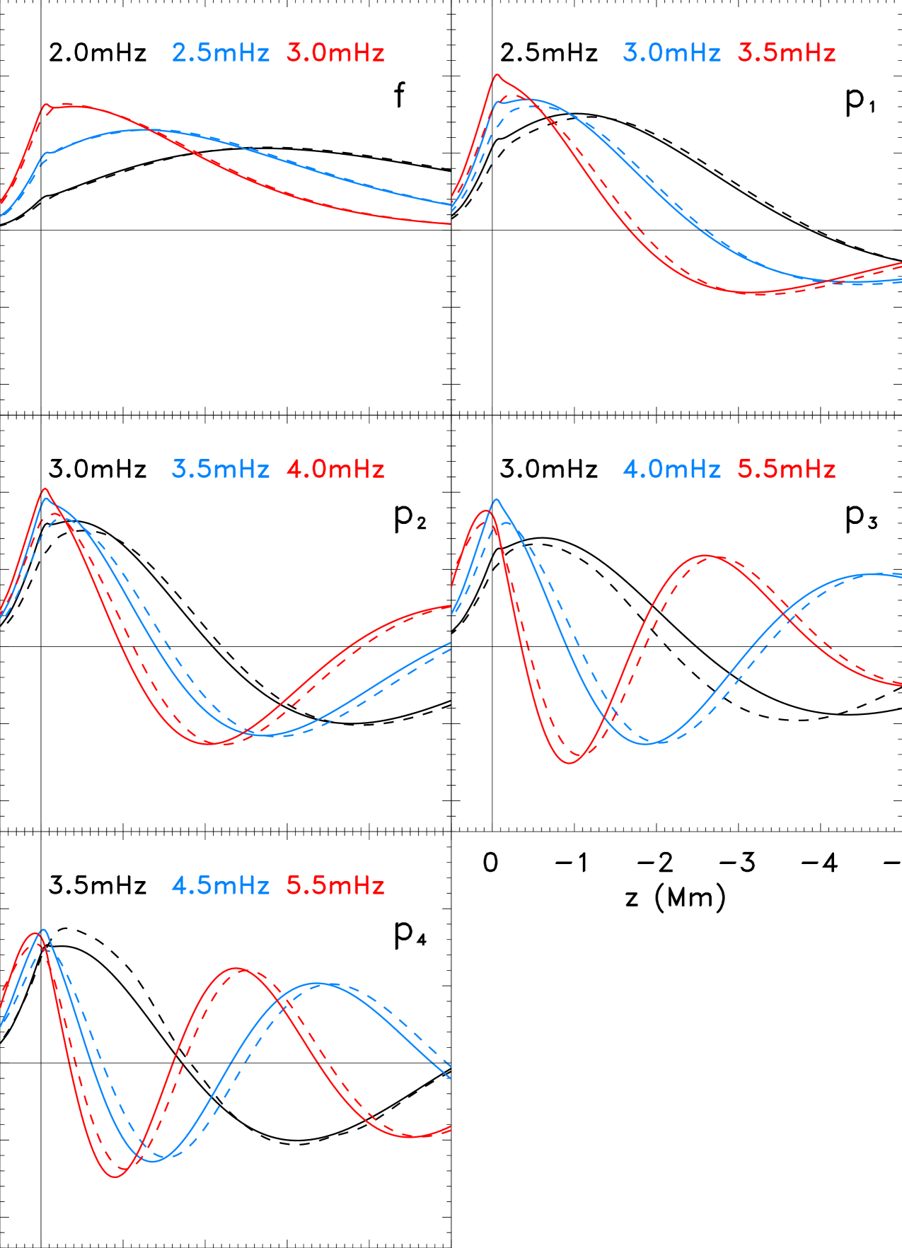
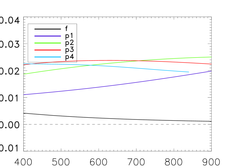
The vertical velocity eigenfunctions of CSM were calculated numerically for each individual mode as described by Schunker et al. (in preparation). The 2D simulation box is 145 Mm in width and covers heights from $z=-20$ Mm to $z=0.7$ Mm (where $z=0$ is the base of the photosphere). The model imposes damping layers above and below to minimise reflection from the boundaries. Due to the height of the box, we are limited to modelling modes with radial orders up to $4$. Figure 1 shows the eigenfunctions for both CSM and Model S for each ridge, f through to p₄, at various frequencies. Figure 2 shows the relative difference between the CSM and Model S eigenfrequencies.

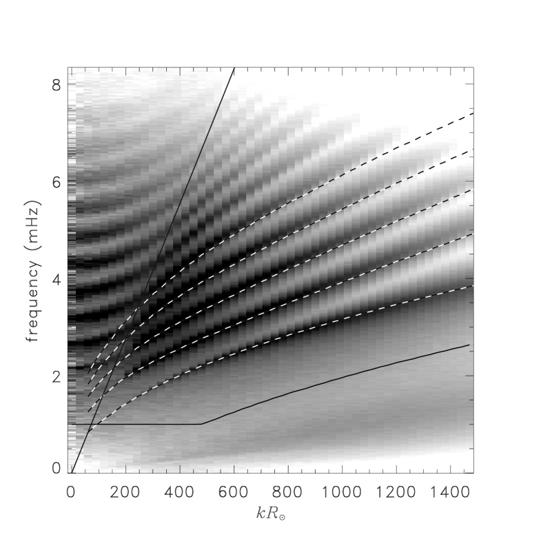
In addition to studying the eigenmodes of the model, we wish to check that the power spectrum of oscillations compares favourably against that of the Sun. We extend the simulation to three dimensions ($145.77\leavevmode\nobreak\ \textrm{Mm}\times 145.77\leavevmode\nobreak\ \textrm{Mm}\times 27.5\leavevmode\nobreak\ \textrm{Mm}$) and introduce random sources 100 km below the surface. The sources are spatially uncorrelated and have an auto-correlation function $\exp(-t^{2}/2\tau^{2})$ where $t$ is the correlation time lag and $\tau=5.5$ minutes. An additional attenuation term taken from Gizon & Birch (2002) is added in the momentum equation to model the finite lifetimes of the modes. The power spectrum of 8 hours of simulated data is shown in Figure 3. The dashed curves are the eigenfrequencies of Model S. Waves with phase speeds higher than $\omega/k=5.86\times 10^{6}$ cm s^-1 (solid line) cannot expect to be modelled correctly because they hit the bottom of the simulation box. When comparing with real solar observations, we find the agreement encouraging: for example, the mode asymmetries and location of the mode ridges compare well, but the mode amplitudes and line-widths could still be improved.

In short, we have constructed a background solar model which is convectively stable, solar-like, and can be used in local helioseismology studies. Opportunities to further improve this model remain and Schunker et al. (in preparation) present a second convectively stabilised model with improved eigenfrequencies.