Convergence analysis of exponential time differencing scheme for the nonlocal Cahn-Hilliard equation
Abstract
In this paper, we present a rigorous proof of the convergence of first order and second order exponential time differencing (ETD) schemes for solving the nonlocal Cahn-Hilliard (NCH) equation. The spatial discretization employs the Fourier spectral collocation method, while the time discretization is implemented using ETD-based multistep schemes. The absence of a higher-order diffusion term in the NCH equation poses a significant challenge to its convergence analysis. To tackle this, we introduce new error decomposition formulas and employ the higher-order consistency analysis. These techniques enable us to establish the bound of numerical solutions under some natural constraints. By treating the numerical solution as a perturbation of the exact solution, we derive optimal convergence rates in . We conduct several numerical experiments to validate the accuracy and efficiency of the proposed schemes, including convergence tests and the observation of long-term coarsening dynamics.
keywords:
Nonlocal Cahn-Hilliard equation, exponential time differencing, Convergence analysis, higher-order consistency analysis.Declarations of interest: none.
1 Introduction
The Cahn-Hilliard (CH) equation was originally proposed in [6] as one of the most typical phase field models which provides a macroscopic description of phase separation and microstructure evolution in binary alloy systems. As a nonlocal variant of the classic CH equation, the Nonlocal Cahn-Hilliard (NCH) equation has attracted increasing attention and has been widely applied in diverse fields ranging from chemistry, material science and image processing [20, 14, 1, 16, 2]. In this paper, we consider the following NCH equation with the periodic boundary conditions [2, 9]:
| (1.1) |
where is a rectangular domain in and is an order parameter subject to the initial condition , is the terminal time, is an interfacial parameter. The function and is a double well function. The nonlocal linear operator is defined by:
| (1.2) |
where is a nonnegative, -periodic radial kernel function and has a finite second moment in .
The linear operator with the kernel function is self-adjoint and positive semi-definite. Further, if is integrable, then , where
| (1.3) |
We assume to ensure the NCH equation (1.1) is positive diffusive [4, 3].
The NCH equation (1.1) can be view as the gradient flow with respect to the free energy functional
| (1.4) |
where denotes the standard inner product on . For the smooth solutions of (1.1), the total mass is conserved:
| (1.5) |
In this paper, we will only consider initial data with mean zero. Then, the fractional Laplacian operator for is well defined [25]. Due to the gradient structure of (1.1), the energy dissipation laws hold:
| (1.6) |
There have been many works on both theoretical analysis and numerical methods for the NCH equation. In mathematical analysis, the well-posedness of the NCH equation equipped with a Neumann or Dirichlet boundary conditions were studied in [3, 4] with an integrable kernel function and in [19] claimed that the existence and uniqueness of the solution to the NCH equation subject to the periodic boundary condition may be established by using a similar technique.
For numerical methods, because of the energetic variational structure inherent in the nonlocal phase field model, an important fact is that the exact solution decrease the energy in time to NCH equation. Therefore, it is essential to develop the so called energy stable numerical algorithms share this key property at the discrete time level. Energy stable numerical schemes of the NCH equation including convex splitting schemes [19, 18], exponential time differencing (ETD) schemes [30, 31, 15], stabilized schemes [9, 27, 28], and so on.
The convergence of numerical solution to NCH equation are established in [19, 17, 26, 27, 28]. In [19, 17], convex splitting schemes were introduced for the NCH equation, demonstrating energy stability and convergence properties. These schemes handled the nonlinear term implicitly and the nonlocal term explicitly, leading to effective numerical solutions but nonlinear iterations were required. Du et al. proposed energy-stable linear semi-implicit schemes in [9], utilizing stabilization techniques to avoid nonlinear iterations. The work in [26] presented the convergence in the discrete norm and established the bound of the numerical solutions for the first-order stabilized linear semi-implicit scheme proposed in [9]. Furthermore, Li et al. [27, 28] developed two energy-stable and convergent second-order linear numerical schemes for the NCH equation. These schemes involved combining a modified Crank-Nicolson (CN) approximation with the Adams-Bashforth extrapolation and stability of the second-order backward differentiation formula (BDF2) for the time discretization, resulting in accurate and stable numerical solutions for the NCH equation.
However, the convergence analysis of ETD schemes for the NCH equation is more challenging and there are currently no results, one of the reasons being that the lack of higher-order diffusion term and the Laplacian of nonlinear term. The ETD schemes [5, 7, 12, 13, 21], which involve exact integration of the target equation followed by an explicit approximation of the temporal integral of the nonlinear term. Exact evaluation of the linear terms makes the ETD schemes achieve high accuracy and satisfactory stability when dealing with stiff differential equations. The first- and second-order ETD schemes were applied to the Nonlocal Allen-Cahn equation and have been analyzed energy stable and convergence [10], and further extended to a class of semi-linear parabolic equations [11]. Convergence and the bound of numerical solutions were proved of ETD schemes to classic CH equation [24].
Compare with the classic CH equation or Nonlocal Allen-Cahn equation, the NCH equation equipped with nonlocal diffusion operator and has more complicated nonlinear term, so that the analytical techniques mentioned above are hardly applicable to the NCH equation. In this paper, we establish the convergence of the fully discrete first-order ETD scheme (ETD1) and second-order ETD multistep scheme (ETD2) for the NCH equation which are developed our recent work [31]. Our analysis is mainly based on two important observations:
- 1.
- 2.
Based on the above two points, we prove the convergence in the discrete norm and obtain the bound of numerical solutions under some natural constraints on the space-time step sizes.
The rest of this paper is organized as follows. The fully discrete ETD1 and ETD2 schemes are constructed in Section 2, and some notations, definitions and useful lemmas are also introduced. In Section 3, we prove the convergence by the higher-order consistency estimate. In addition, the bound of numerical solutions are also obtained. In Section 4, some numerical experiments are carried out to test the convergence in time level. The coarsening dynamics are simulated to show the long time behaviors of ETD2. Some concluding remarks are given in Section 5.
2 Fully discrete exponential time differencing schemes
In this section, we present the fully discrete exponential time differencing schemes for the NCH equation, where the Fourier spectral collocation method is adopted for the spatial discretization.
We consider the square domain and define the spatial grid where the space step size ( is even). We need two spaces. Let be the space of all the -periodic grid functions. That means if , then is a discrete function defined on the discrete grid . Let be the space of the zero-mean grid functions. That means if , then , where is the index set defined in the Appendix A.
We denote and are Fourier spectral collocation space approximation operators of and . These detailed definitions and some related properties are given in the Appendix A. For any , the discrete inner product , and norm , , , and the discrete convolution are defined in the Appendix A.
It is well known [12] that a suitable linear operator splitting can improve the stability. So we can introduce a stabilizing parameter and define
| (2.1) |
Now is self-adjoint and positive definite on . Then the space semi-discrete equation for (1.1) is to find such that
| (2.2) |
where the initial value is given.
Let , where is the time step size and is a given positive integer. By using the property of the differentiation of matrix exponentials, the solution of the equation (2.2) satisfies
| (2.3) |
The key to construct the ETD schemes is to approximate the nonlinear term in (2.3) by polynomial interpolation, and then precisely integrate the interpolation.
The ETD1 scheme comes from approximating by the constant , given by
| (2.4) |
where . The ETD2 scheme is obtained by approximating by a linear extrapolation based on and , given by
| (2.5) |
where
The ETD2 scheme (2.5) is a two-step algorithm, an accurate approximation for the value at is needed. Usually, can be computed by the ETD1. But in this paper, we choose a higher-order approximation for , to facilitate the higher-order consistency analysis presented in the later sections. For example, we can apply the second-order Runge-Kutta (RK2) method in first step, which yields a third-order temporal accuracy at for exact initial data .
The following lemmas are useful in our following convergence analysis.
Lemma 2.2 ([9]).
The operator has the following properties:
(i) the eigenvalues of are ;
(ii) commutes with and is self-adjoint and positive semi-define;
(iii) for any , we have .
Lemma 2.3 ([26]).
Suppose and define its gird restriction via . Then for any and , we have
| (2.6) |
where is a positive constant that depends on and but is independent of .
3 Convergence analysis
In this section, we analyze the convergence of the ETD1 scheme and ETD2 scheme, and give an optimal rate error estimates in . To perform the convergence analysis, let’s first introduce the concept and preliminary.
For a linear symmetric operator , we define the norm by the spectrum radius of , i.e., , where is the set of all the eigenvalues of . It holds that
Denote by the exact solution of (1.1). The existence and uniqueness of may be obtained by using the techniques adopted in [3, 4], from which one can get the following estimate
| (3.1) |
Moreover, if the initial data is sufficient regularity, we can assume that the exact solution has regularity as
| (3.2) |
Let be the space of trigonometric polynomials of degree up to . Let be the orthogonal projection operator. We define . If for some , the following estimate is standard [29]
| (3.3) |
By the orthogonality of Fourier projection , we have . Noting that the exact solution is mass conservative, i.e., . Thus, we obtain
| (3.4) |
Since , we have , that means the rectangular quadrature rule holds exactly for all . The values of at discrete grid points are still denoted as , i.e., . Recall then from (3.4) we can get the mass conservative property of in the discrete average sense:
On the other hand, the solutions of the numerical schemes (2.4)-(2.5) are also mass conservative [30]: We use the mass conservative for the initial value , and define the error grid function
| (3.5) |
We have , so is well defined. Under the regularity assumption (3.1), for the projection functions , we have
| (3.6) |
The main result of this work is the following theorem.
Theorem 3.1.
Assume that the solution of the NCH equation (1.1) satisfying the regularity class presented in (3.2). Also assume that and are small sufficiently and satisfy for some constant . Let .
(i) For ETD1 scheme, if the stabilizing parameter , we have
| (3.7) |
(ii) For ETD2 scheme, if the stabilizing parameter , we have
| (3.8) |
where are some positive constant and are independent of and .
We provide a heuristic explanation of the main idea behind the proof. The usual convergence analysis starts directly from the error equation defined in (3.5). However, our here adopts a new strategy. We construct two new error decomposition representation formulas
| (3.9) |
where and is the constructed approximate solution defined in (3.14) for the ETD1 scheme and in (3.37) for the ETD2 scheme, , and are temporal correction functions. By doing so, we can obtain an truncation error. This higher consistency allows us to derive a higher order convergence estimate of the modified error function as (see (3.31) and (3.49)), which in turn lead to under reasonable condition . Due to the lack of higher-order diffusion term, we adopt to test the error function in (3.23) and (3.2.2), instead of as that in [24]. Then, we estimate both sides of the error equation by using the result of the higher-order consistency analysis and induction argument, we can obtain an optimal convergence rate in for of the proposed two numerical schemes.
3.1 Convergence analysis of ETD1
3.1.1 Higher-order consistency analysis
For a given , the solution of the ETD1 scheme (2.4) can be given by with the function determined by the following evolution equation:
| (3.10) |
Then, for the continuous NCH equation (1.1), we can give a similar expression as follows. For given , the solution can be obtained by with the function satisfying
| (3.11) |
Denote the function . Then satisfies the following equation:
| (3.12) |
and also solves the discrete equation (3.10) with the local truncation error
| (3.13) |
By comparing equations (3.12) and (3.13), we can get where
By the standard Fourier spectral approximation, has the bound . By Taylor expansion with the integral remainder, can be bounded by . Thus, we have
Since the local truncation error only has first order accuracy in time, it is not enough to derive the boundedness of numerical solution, i.e., . To remedy this, we introduce the auxiliary profile
| (3.14) |
where and are two temporal correction functions will be constructed later. By doing so, we can obtain a higher consistency.
Let’s construct the correction function first. By Fourier projection from continuous NCH equation (1.1) and carry out the space discretization, we have satisfying
Expansing the nonlinear term for at to obtain , where depends only on and . We get that
| (3.15) |
By mass conservative and the periodic boundary condition, we also have .
The first order temporal correction function is given by solving the following ODE system:
| (3.16) |
The existence and uniqueness of the solution of this linear system is standard and it depends only on .
Let . Then it follows from the equations (3.15) and (3.16) that
| (3.17) |
where we have used the following expansion
and defined in (3.17) depends only on and . We also have . Similarly, we can get the second order temporal correction function , which is the solution of the following linear ODE system:
| (3.18) |
The unique solution only dependent on . Define a grid function . Combination of (3.17) and a Fourier projection of (3.18) leads to
| (3.19) |
where we have used the fact
We see that . Thus, we have completed the construction of .
Note that is also bounded. In fact, it follows from and that In particular, when is sufficiently small we have , which gives
3.1.2 Convergence analysis in
Let for . Then, by consistency, satisfies
| (3.20) |
where the truncation error satisfies
| (3.21) |
Subtracting (3.20) from (3.10) and putting yield
| (3.22) |
Hence, satisfies that
| (3.23) |
Acting on (3.23) and taking the discrete inner product with yield
| (3.24) |
where
| (3.25) |
Next, we use induction argument to prove the convergence. We note that numerical error function at . Suppose at . Thus, the bound for the numerical solutions at becomes available:
We now estimate the three terms on the right-hand side given in (3.1.2). For the first linear term, a direct application of Cauchy inequality and Lemma 2.1 give
| (3.26) |
By noting that , we have
where between and and . Then, for the second term in (3.1.2), by using Lemma 2.1 and the above estimate, we have
| (3.27) |
For the last term in (3.1.2), we have the following estimate:
| (3.28) |
For the nonlocal linear term given in (3.24), by appling Lemma 2.2 and Lemma 2.3, we obtain
| (3.29) |
where depends on and .
Therefore, a substitution of (3.1.2)-(3.1.2) and (3.1.2) into (3.24), and recall the define of , we get
| (3.30) |
Summing the above inequality from 0 to leads to
Subsequently, assuming that and putting , we can apply the discrete Gronwall’s inequality to obtain the following convergence estimate:
| (3.31) |
where depends on . By using the inverse inequality to (3.31), the following estimate holds
| (3.32) |
provided that , where we assumed and the fact that . Then, we have
| (3.33) |
This completes the error estimate for error function .
3.2 Convergence analysis of ETD2
Similar to the proof of convergence of ETD1 scheme in subsection 3.1, we next prove the convergence of the ETD2 scheme.
3.2.1 Higher-order consistency analysis
Similar to the higher-order consistency analysis of the ETD1 scheme, the Fourier projection solution satisfies the following equation:
| (3.36) |
where the function depends only on and and we have . Define the auxiliary profile
| (3.37) |
where the temporal correction function solves the following linear ODE system:
| (3.38) |
subject to the zero initial value. Note that the solution of (3.2.1) exists and is unique and the solution is smooth enough. Combination of (3.36) and (3.2.1) gives the higher-order consistency estimate:
| (3.39) |
where we have used the estimate
We also have and the boundedness of . In fact, by noting and if is small sufficiently, we have And if we adopt the RK2 numerical algorithm for the estimate of , it holds that
3.2.2 Convergence analysis in
For given , the solution of the ETD2 scheme (2.5) is actually given by with the function determined by the evolution equation:
| (3.40) |
The function satisfies (3.40) with the truncated error
| (3.41) |
where satisfies
Let . The difference between (3.40) and (3.41) gives
| (3.42) |
Thus, the solution satisfies that
| (3.43) |
Acting on both sides of (3.2.2) and taking inner product of the resulted equation with yield
| (3.44) |
where
By induction argument, assuming for the numerical error function at the previous time steps and satisfy
| (3.45) |
then we have Based on the above assumptions and , we have
We now estimate defined in (3.44). By Lemma 2.1 and Cauchy inequality, we obtain
| (3.46) |
Then, a substitution (3.2.2) and (3.1.2) to (3.44), we obtain
| (3.47) |
Summing the above inequality from 1 to leads to
| (3.48) |
Then using the estimate and assuming that and , an application of the discrete Gronwall’s inequality gives the convergence result:
| (3.49) |
where is depends on and but independent of and . Similar to the estimation of (3.32) and (3.33), we can get and provided that .
4 Numerical experiments
In this section, we present numerical experiments to verify the temporal convergence rates in the discrete norm of the proposed ETD1 and ETD2 schemes. We also investigate the phase transition till the steady state and simulate the coarsening dynamics to show the longtime behavior for the NCH equation (1.1). Set for the ETD1 scheme and for the ETD2 scheme in all experiments. We use the Guass-type function [9, 31]
where is a parameter. Note that , then is equivalent to .
4.1 Convergence tests
Example 4.1 (2D test).
We consider the NCH equation (1.1) on subject to the periodic boundary condition with the initial value .
In order to test the time accuracy of the numerical methods, we calculate the -norm error using
and the time convergence order by .
In this simulation and . We compute the numerical solutions for ETD1 and ETD2 schemes with various time step sizes . The reference solutions is taken as the approximated solution obtained with a quite small time step size . The errors and convergence rates in the discrete norm are showed in Table 1 and Table 2, which shows the first order of accuracy for the ETD1 scheme and the second order of accuracy for the ETD2 scheme with different and , as expected.
| ETD1 | |||||
|---|---|---|---|---|---|
| error | Rate | error | Rate | ||
| 5.1108E-05 | – | 7.2409E-05 | – | ||
| 2.1838E-05 | 1.2267 | 2.1994E-05 | 1.7191 | ||
| 1.0061E-05 | 1.1181 | 8.7574E-06 | 1.3285 | ||
| 4.8154E-06 | 1.0630 | 3.9203E-06 | 1.1595 | ||
| 2.3443E-06 | 1.0385 | 1.8485E-06 | 1.0846 | ||
| 1.1456E-06 | 1.0331 | 8.8928E-07 | 1.0556 | ||
| 5.5526E-07 | 1.0448 | 4.2773E-07 | 1.0560 | ||
| 2.6235E-07 | 1.0817 | 2.0132E-07 | 1.0872 | ||
| 1.1645E-07 | 1.1718 | 8.9191E-08 | 1.1745 | ||
| ETD2 | |||||
|---|---|---|---|---|---|
| error | Rate | error | Rate | ||
| 1.1417E-05 | – | 1.8032E-06 | – | ||
| 2.5795E-06 | 2.1461 | 3.9009E-07 | 2.2087 | ||
| 6.2025E-07 | 2.0562 | 8.8718E-08 | 2.1365 | ||
| 1.5266E-07 | 2.0225 | 2.0981E-08 | 2.0801 | ||
| 3.7907E-08 | 2.0098 | 5.0878E-09 | 2.0040 | ||
| 9.4434E-09 | 2.0051 | 1.2512E-09 | 2.0238 | ||
| 2.3530E-09 | 2.0048 | 3.0946E-10 | 2.0155 | ||
| 5.8343E-10 | 2.0119 | 7.6282E-11 | 2.0203 | ||
| 1.4140E-10 | 2.0448 | 1.8444E-11 | 2.0482 | ||
Example 4.2 (3D test).
In this test, we calculate the errors and convergence rates by ETD2 scheme for the NCH equation on the computational domain . We choose the same and as 2D.
We consider the smooth initial condition , the computational results are presented in Table 3. From Table 3 one can see that time accuracy is second order, which is onsistent with our theoretical predictions.
| ETD2 | |||||
|---|---|---|---|---|---|
| error | Rate | error | Rate | ||
| 1.8586E-05 | – | 2.8680E-05 | – | ||
| 3.5861E-06 | 2.3737 | 2.4139E-06 | 3.5706 | ||
| 8.1176E-07 | 2.1433 | 2.6908E-07 | 3.1652 | ||
| 1.9593E-07 | 2.0507 | 4.4968E-08 | 2.5811 | ||
| 4.8344E-08 | 2.0189 | 9.7783E-09 | 2.2012 | ||
| 1.2017E-08 | 2.0082 | 2.3470E-09 | 2.0587 | ||
| 2.9918E-09 | 2.0060 | 5.7920E-10 | 2.0187 | ||
| 7.4157E-10 | 2.0123 | 1.4335E-10 | 2.0146 | ||
| 1.7970E-10 | 2.0450 | 3.4806E-11 | 2.0421 | ||
4.2 Interfaces in the steady states
We now simulate the shapes of the interfaces formed in the steady states by the NCH equation (1.1) under the ETD2 scheme in one-dimensional case with various and .
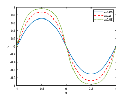
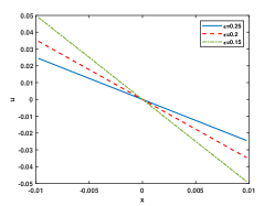
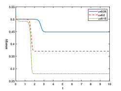
Example 4.3 (1D problem).
Let , , and .
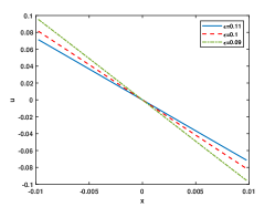
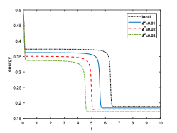
In Figure 2, we fix and choose as 0.25, 0.2, 0.15, 0.11, 0.1 and 0.09. We plot the numerical solutions at the steady states and the curve of discrete energy evolution. The Figure shows that the numerical solutions reach the steady state at and , respectively. The energy stability of the ETD2 can be seen in the last column. It is observed that the time required to reach the steady state increases as decreases and the interface width becomes sharper for smaller .
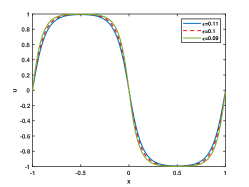
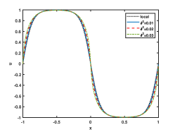
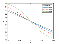
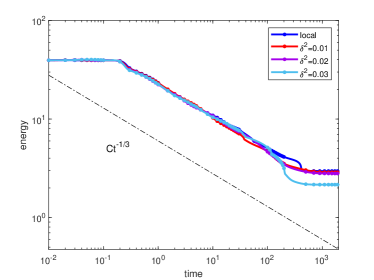
In Figure 2, we choose , and as 0.03, 0.02, 0.01 respectively. Furthermore, we simulate the local CH equation for comparison. From Figure 2, we observe the energy curve remain unchanged after and the numerical solutions reach the steady state in this time. As decreases, the interface turns flat, and the phase transition process is close to the local one for all cases.

4.3 Coarsening dynamics and energy evolution
Example 4.4 (2D problem).
We now simulate the long time behavior of the NCH equation (1.1) by using the ETD2 scheme in with a random initial data ranging from -0.1 to 0.1. We set time step size and choose .
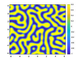
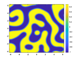
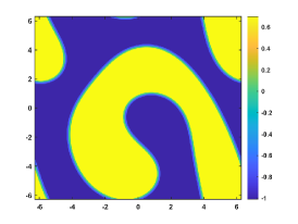
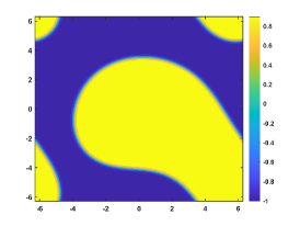

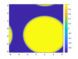
Let . Figure 4 shows the coarsening dynamics of numerical solutions, from which one can observe that the dynamic evolves from the initial disorder state to the ordered states and reach the steady state around .
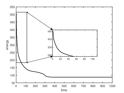
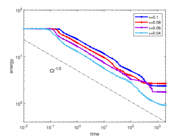
Let and , respectively. Figure 4(a) plots the energy evolution curves, and we can observe the energy decay rates comply with the power law for all cases. This is consistent to the local CH equation [8, 23]. We also plot the curves of the energy for with different in Figure 4(b). Table 4 presents the linear fitting coefficients and for decreasing from to with the fitting function .
| 0.1 | 0.09 | 0.08 | 0.07 | 0.06 | 0.05 | 0.04 | |
|---|---|---|---|---|---|---|---|
| -0.314 | -0.314 | -0.325 | -0.331 | -0.303 | -0.320 | -0.341 | |
| 21.08 | 19.49 | 18.15 | 17.13 | 15.04 | 13.46 | 12.64 |
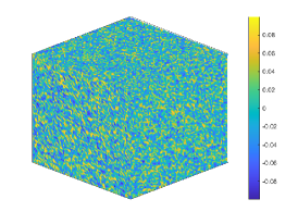
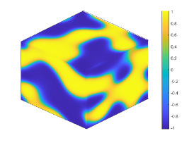
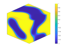
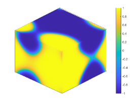
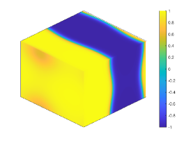
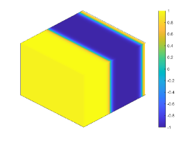
Example 4.5 (3D problem).
We perform the coarsening dynamics of the numerical solutions in 3D on the domain with initial data . Set , and .
5 Conclusion remarks
Because of the non-locality and nonlinearity, it is very challenging to prove the convergence of numerical methods for NCH equation. In this paper, we provide a detailed convergence analysis of the ETD1 and ETD2 schemes for the NCH equation, where the Fourier spectral collocation method is used for the spatial discretizations. Due to the lack of the higher-order diffusion term, we adopt as the test function rather than in the classic CH equation for error equations. The optimal convergence rates in discrete norm have been presented by performing the high order consistency analysis. In addition, we also obtain bound of the numerical solutions under some moderate constraints on the space-time step sizes. Finally, we verify the convergence in time of the proposed schemes numerically and simulate the coarsening dynamics to show the long time behavior and present the power law for the energy decay for the NCH equation.
Appendix A: Fourier spectral collocation Approximations
We introduce some notations and useful properties of Fourier spectral collocation approximations for space local linear operators and nonlocal operator in two dimension. Define the index sets
The space of all the -periodic grid functions is denoted by . For any , the discrete inner product and norm and discrete norm are, respectively, defined by
For a function , we have discrete Fourier transform [29]
| (5.1) |
where
| (5.2) |
are the discrete Fourier coefficients. The first and second order derivatives of in the direction can be defined as
The differentiation operators in the direction can be defined in the same way. For any , the discrete gradient and Laplace operators are given by
| (5.3) |
For any , we have the following summation-by-parts formulas [22]
For any , we call the mean value of . By noticing (1.5) and assuming that the mean of is zero, we only need to consider the zero-mean grid functions, i.e.,
where . Similar to the continuous case, is self-adjoint and positive definite on and thus is well-defined and is also self-adjoint and positive definite. Then for any , we can define the discrete inner produce and the discrete norm as
For any , the discrete convolution can be defined componentwise [9] by
Given a kernel function satisfying the conditions, then for any , the discrete form of nonlocal diffusion operator can be defined by with
| (5.4) |
where is a discrete Fourier transform matrix and
References
- AE [04] A. Archer and R. Evans. Dynamical density functional theory and its application to spinodal decomposition. J. Chem. Phys., 121:4246–4254, 2004.
- Bat [06] P. W. Bates. On some nonlocal evolution equations arising in materials science. Fields Inst. Commun., 48:13–52, 2006.
- [3] P. W. Bates and J. L. Han. The Dirichlet boundary problem for a nonlocal Cahn-Hilliard equation. J. Math. Anal., 311:289–312, 2005.
- [4] P. W. Bates and J. L. Han. The Neumann boundary problem for a nonlocal Cahn-Hilliard equation. J. Differ. Equa., 212:235–277, 2005.
- BKV [98] G. Beylkin, J. M. Keiser, and Lev. Vozovoi. A new class of time discretization schemes for the solution of nonlinear PDEs. J. Comput. Phys., 147(2):362–387, 1998.
- CH [58] J. W. Cahn and J. E. Hilliard. Free energy of a nonuniform system. I. Interfacial free energy. J. Chem. Phys., 28(2):258–267, 1958.
- CM [02] S. M. Cox and P. C. Matthews. Exponential time differencing for stiff systems. J. Comput. Phys., 176(2):430–455, 2002.
- DD [16] S. B. Dai and Q. Du. Computational studies of coarsening rates for the Cahn–Hilliard equation with phase-dependent diffusion mobility. J. Comput. Phys., 310:85–108, 2016.
- DJLQ [18] Q. Du, L. L. Ju, X. Li, and Z. H. Qiao. Stabilized linear semi-implicit schemes for the nonlocal Cahn–Hilliard equation. J. Comput. Phys., 363:39–54, 2018.
- DJLQ [19] Q. Du, L. L. Ju, X. Li, and Z. H. Qiao. Maximum principle preserving exponential time differencing schemes for the nonlocal Allen–Cahn equation. SIAM J. Numer. Anal., 57(2):875–898, 2019.
- DJLQ [21] Q. Du, L. L. Ju, X. Li, and Z. H. Qiao. Maximum bound principles for a class of semilinear parabolic equations and exponential time-differencing schemes. SIAM Review., 63(2):317–359, 2021.
- DZ [04] Q. Du and W. X. Zhu. Stability analysis and application of the exponential time differencing schemes. J. Comput. Math., 22(2):200–209, 2004.
- DZ [05] Q. Du and W. X. Zhu. Analysis and applications of the exponential time differencing schemes and their contour integration modifications. BIT Numerical. Mathematics., 45:307–328, 2005.
- Fif [03] P. Fife. Some Nonclassical Trends in Parabolic and Parabolic-like Evolutions, Trends in Nonlinear Analysis. Springer, Berlin., 2003.
- FSY [24] Z. H. Fu, J. Shen, and J. Yang. Higher-Order Energy-Decreasing Exponential Time Differencing Runge-Kutta methods for Gradient Flows. arXiv preprint arXiv:2402.15142, 2024.
- GG [05] H. Gajewski and K. Gärtner. On a nonlocal model of image segmentation. Z. Angew. Math. Phys., 56:572–591, 2005.
- GLW [17] Z. Guan, J. Lowengrub, and C. Wang. Convergence analysis for second-order accurate schemes for the periodic nonlocal Allen-Cahn and Cahn-Hilliard equations. Math. Methods Appl. Sci., 40(18):6836–6863, 2017.
- GLWW [14] Z. Guan, J. Lowengrub, C. Wang, and S. M. Wise. Second order convex splitting schemes for periodic nonlocal Cahn–Hilliard and Allen–Cahn equations. J. Comput. Phys., 277:48–71, 2014.
- GWW [14] Z. Guan, C. Wang, and S. M. Wise. A convergent convex splitting scheme for the periodic nonlocal Cahn-Hilliard equation. Numer Math., 128:377–406, 2014.
- HKV [01] D. J. Horntrop, M. A. Katsoulakis, and D. G. Vlachos. Spectral methods for mesoscopic models of pattern formation. J. Comput. Phys., 173:364–390, 2001.
- HO [10] M. Hochbruck and A. Ostermann. Exponential integrators. Acta Numerica., 19:209–286, 2010.
- JLQZ [18] L. L. Ju, X. Li, Z. H. Qiao, and H. Zhang. Energy stability and error estimates of exponential time differencing schemes for the epitaxial growth model without slope selection. Math Comput., 87(312):1859–1885, 2018.
- JZD [15] L. L. Ju, J. Zhang, and Q. Du. Fast and accurate algorithms for simulating coarsening dynamics of Cahn–Hilliard equations. Comput. Mater. Sci., 108:272–282, 2015.
- LJM [19] X. Li, L. L. Ju, and X. C. Meng. Convergence analysis of exponential time differencing schemes for the Cahn-Hilliard equation. Commun. Comput. Phys., 26(5):1510–1529, 2019.
- LQT [16] D. Li, Z. H. Qiao, and T. Tang. Characterizing the stabilization size for semi-implicit Fourier-spectral method to phase field equations. SIAM J. Numer. Anal., 54(3):1653–1681, 2016.
- LQW [21] X. Li, Z. H. Qiao, and C. Wang. Convergence analysis for a stabilized linear semi-implicit numerical scheme for the nonlocal Cahn–Hilliard equation. Math Comput., 90(327):171–188, 2021.
- LQW [23] X. Li, Z. H. Qiao, and C. Wang. Stabilization parameter analysis of a second-order linear numerical scheme for the nonlocal Cahn–Hilliard equation. SIAM J. Numer. Anal., 43(2):1089–1114, 2023.
- LQW [24] X. Li, Z. H. Qiao, and C. Wang. Double stabilizations and convergence analysis of a second-order linear numerical scheme for the nonlocal Cahn-Hilliard equation. Sci. China. Math., 67(1):187–210, 2024.
- STW [11] J. Shen, T. Tang, and L-L. Wang. Spectral methods: algorithms, analysis and applications. Springer., 2011.
- ZS [23] Q. Zhou and Y. B. Sun. Energy stability of exponential time differencing schemes for the nonlocal Cahn-Hilliard equation. Numer. Methods. Partial. Differ. Equ., 39(5):4030–4058, 2023.
- ZW [24] D. N. Zhang and D. L. Wang. Energy-decreasing second order exponential time differencing Runge–Kutta methods for Nonlocal Cahn–Hilliard equation. Appl. Math. Lett., 150:108974, 2024.