Convergence of the Deep BSDE Method
for Coupled FBSDEs

Forward-backward stochastic differential equations (FBSDEs) and partial differential equations (PDEs) of parabolic type have found numerous applications in stochastic control, finance, physics, etc., as a ubiquitous modeling tool. In most situations encountered in practice the equations cannot be solved analytically but require certain numerical algorithms to provide approximate solutions. On the one hand, the dominant choices of numerical algorithms for PDEs are mesh-based methods, such as finite differences, finite elements, etc. On the other hand, FBSDEs can be tackled directly through probabilistic means, with appropriate methods for the approximation of conditional expectation. Since these two kinds of equations are intimately connected through the nonlinear Feynman–Kac formula [1], the algorithms designed for one kind of equation can often be used to solve another one.

However, the aforementioned numerical algorithms become more and more difficult, if not impossible, when the dimension increases. They are doomed to run into the so-called “curse of dimensionality” [2] when the dimension is high, namely, the computational complexity grows exponentially as the dimension grows. The classical mesh-based algorithms for PDEs require a mesh of size $O(N^{d})$. The simulation of FBSDEs faces a similar difficulty in the general nonlinear cases, due to the need to compute conditional expectation in high dimension. The conventional methods, including the least squares regression [3], Malliavin approach [4], and kernel regression [5], are all of exponential complexity. There are a limited number of cases where practical high-dimensional algorithms are available. For example, in the linear case, Feynman–Kac formula and Monte Carlo simulation together provide an efficient approach to solving PDEs and associated BSDEs numerically. In addition, methods based on the branching diffusion process [6, 7] and multilevel Picard iteration [8, 9, 10] overcome the curse of dimensionality in their considered settings. We refer [9] for the detailed discussion on the complexity of the algorithms mentioned above. Overall there is no numerical algorithm in literature so far proved to overcome the curse of dimensionality for general quasilinear parabolic PDEs and the corresponding FBSDEs.

A recently developed algorithm, called the deep BSDE method [11, 12], has shown astonishing power in solving general high-dimensional FBSDEs and parabolic PDEs [13, 14, 15]. In contrast to conventional methods, the deep BSDE method employs neural networks to approximate unknown gradients and reformulates the original equation-solving problem into a stochastic optimization problem. Thanks to the universal approximation capability and parsimonious parameterization of neural networks, in practice the objective function can be effectively optimized in high-dimensional cases, and the function values of interests are obtained quite accurately.

The deep BSDE method was initially proposed for decoupled FBSDEs. In this paper, we extend the method to deal with coupled FBSDEs and a broader class of quasilinear parabolic PDEs. Furthermore, we present an error analysis of the proposed scheme, including decoupled FBSDEs as a special case. Our theoretical result consists of two theorems. Theorem 1 provides a posteriori error estimation of the deep BSDE method. As long as the objective function is optimized to be close to zero under fine time discretization, the approximate solution is close to the true solution. In other words, in practice, the accuracy of the numerical solution is effectively indicated by the value of the objective function. Theorem 2 shows that such a situation is attainable, by relating the infimum of the objective function to the expression ability of neural networks. As an implication of the universal approximation property (in the $L^{2}$ sense), there exist neural networks with suitable parameters such that the obtained numerical solution is approximately accurate. To the best of our knowledge, this is the first theoretical result of the deep BSDE method for solving FBSDEs and parabolic PDEs. Although our numerical algorithm is based on neural networks, the theoretical result provided here is equally applicable to the algorithms based on other forms of function approximations.

The article is organized as follows. In section 2, we precisely state our numerical scheme for coupled FBSDEs and quasilinear parabolic PDEs and give the main theoretical results of the proposed numerical scheme. In section 3, the basic assumptions and some useful results from the literature are given for later use. The proofs of the two main theorems are provided in section 4 and section 5, respectively. 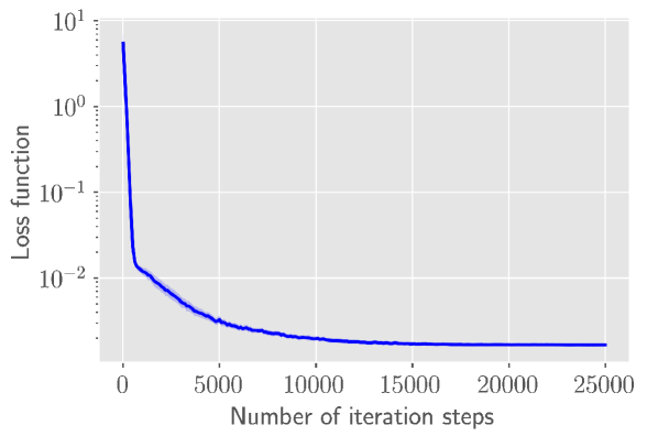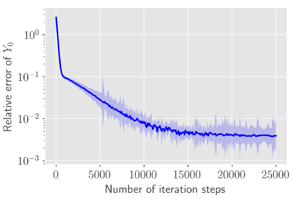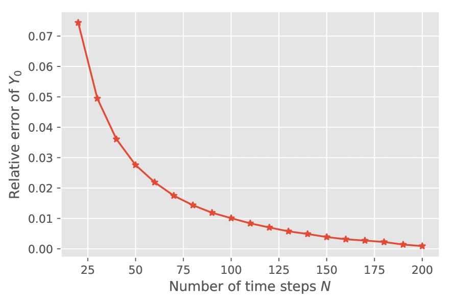Some numerical experiments with the proposed scheme are presented in section 6.

Let $T\in(0,+\infty)$ be the terminal time, $(\Omega,\mathbb{F},\{\mathcal{F}_{t}\}_{0\leq t\leq T},\mathbb{P})$ be a filtered probability space equipped with a $d$-dimensional standard Brownian motion $\{W_{t}\}_{0\leq t\leq T}$ starting from $0$. $\xi$ is a square-integrable random variable independent of $\{W_{t}\}_{0\leq t\leq T}$. We use the same notation $(\Omega,\mathbb{F},\{\mathcal{F}_{t}\}_{0\leq t\leq T},\mathbb{P})$ to denote the filtered probability space generated by $\{W_{t}+\xi\}_{0\leq t\leq T}$. The notation $|x|$ denotes the Euclidean norm of a vector $x$ and $\|A\|=\sqrt{\mathrm{trace}(A^{\operatorname{T}}A)}$ denotes the Frobenius norm of a matrix $A$.

Consider the following coupled FBSDEs

in which $X_{t}$ takes values in $\mathbb{R}^{m}$, $Y_{t}$ takes values in $\mathbb{R}$, and $Z_{t}$ takes values in $\mathbb{R}^{d}$. Here we assume $Y_{t}$ to be one-dimensional to simplify the presentation. The result can be extended without any difficulty to the case where $Y_{t}$ is multi-dimensional. We say $(X_{t},Y_{t},Z_{t})$ is a solution of the above FBSDEs, if all its components are $\mathcal{F}_{t}$-adapted and square-integrable, together satisfying equations (2.1)(2.2).

Solving coupled FBSDEs numerically is more difficult than solving decoupled FBSDEs. Except the Picard iteration method developed in [16], most methods exploit the relation to quasilinear parabolic PDEs via the four-time-step-scheme in [17]. This type of methods suffers from high dimensionality due to spatial discretization of PDEs. In contrast, our strategy, starting from simulating the coupled FBSDEs directly, is a new purely probabilistic scheme. To state the numerical algorithm precisely, we consider a partition of the time interval $[0,T]$, $\pi:0=t_{0}<t_{1}<\dots<t_{N}=T$ with $h=T/N$ and $t_{i}=ih$. Let $\Delta W_{i}\coloneqq W_{t_{i+1}}-W_{t_{i}}$ for $i=0,1,\dots,N-1$. Inspired by the nonlinear Feynman–Kac formula that will be introduced below, we view $Y_{0}$ as a function of $X_{0}$ and view $Z_{t}$ as a function of $X_{t}$ and $Y_{t}$. Equipped with this viewpoint, our goal becomes finding appropriate functions $\mu_{0}^{\pi}:\mathbb{R}^{m}\rightarrow\mathbb{R}$ and $\phi_{i}^{\pi}:\mathbb{R}^{m}\times\mathbb{R}\rightarrow\mathbb{R}^{d}$ for $i=0,1,\dots,N-1$ such that $\mu_{0}^{\pi}(\xi)$ and $\phi_{i}^{\pi}(X_{t_{i}}^{\pi},Y_{t_{i}}^{\pi})$ can serve as good surrogates of $Y_{0}$ and $Z_{t_{i}}$, respectively. To this end, we consider the classical Euler scheme

Without loss of clarity, here we use the notation $X_{0}^{\pi}$ as $X_{t_{0}}^{\pi}$, $X_{T}^{\pi}$ as $X_{t_{N}}^{\pi}$, etc.

Following the spirit of the deep BSDE method, we employ a stochastic optimizer to solve the following stochastic optimization problem

where $\mathcal{N}^{\prime}_{0}$ and $\mathcal{N}_{i}\leavevmode\nobreak\ (0\leq i\leq{N-1})$ are parametric function spaces generated by neural networks. To see intuitively where the objective function (2.4) comes from, we consider the following variational problem:

where $Y_{0}$ is $\mathcal{F}_{0}$-measurable and square-integrable, and $Z_{t}$ is a $\mathcal{F}_{t}$-adapted square-integrable process. The solution of the FBSDEs (2.1)(2.2) is a minimizer of the above problem since the loss function attains zero when it is evaluated at the solution. In addition, the wellposedness of the FBSDEs (under some regularity conditions) ensures the existence and uniqueness of the minimizer. Therefore, we expect (2.4), as a discretized counterpart of (2.5), defines a benign optimization problem and the associated near-optimal solution provides us a good approximate solution of the original FBSDEs. The reason we do not represent $Z_{t_{i}}$ as a function of $X_{t_{i}}$ only is that the process $\{X_{t_{i}}^{\pi}\}_{0\leq i\leq N}$ is not Markovian, while the process $\{X_{t_{i}}^{\pi},Y_{t_{i}}^{\pi}\}_{0\leq i\leq N}$ is Markovian, which facilitates our analysis considerably. If $b$ and $\sigma$ are both independent of $Y$, then the FBSDEs (2.1)(2.2) are decoupled, we can take $\phi_{i}^{\pi}$ as a function of $X_{t_{i}}^{\pi}$ only, as the numerical scheme introduced in [11, 12].

Our two main theorems regarding the deep BSDE method are the following, mainly on the justification and property of the objective function (2.4) in the general coupled case, regardless of the specific choice of parametric function spaces. An important assumption for the two theorems is the so-called weak coupling or monotonicity condition, which will be explained in detail in section 3. The precise statement of the theorems can be found in Theorem 1^′ (section 4) and Theorem 2^′ (section 5), respectively.

Briefly speaking, Theorem 1 states that the simulation error (left side of equation (2.6)) can be bounded through the value of the objective function (2.4). To the best of our knowledge, this is the first result for the error estimation of the coupled FBSDEs, concerning both time discretization error and terminal distance. Theorem 2 states that the optimal value of the objective function can be small if the approximation capability of the parametric function spaces ($\mathcal{N}^{\prime}_{0}$ and $\mathcal{N}_{i}$ above) is high. Neural networks are a promising candidate for such a requirement, especially in high-dimensional problems. There are numerous results, dating back to the 90s (see, e.g., [18, 19, 20, 21, 22, 23, 24, 25, 26, 27]), in regard to the universal approximation and complexity of neural networks. There are also some recent analysis [28, 29, 30, 31] on approximating the solutions of certain parabolic partial differential equations with neural networks. However, the problem is still far from resolved. Theorem 2 implies that if the involved conditional expectations can be approximated by neural networks whose numbers of parameters growing at most polynomially both in the dimension and the reciprocal of the required accuracy, then the solutions of the considered FBSDEs can be represented in practice without the curse of dimensionality. Under what conditions this assumption is true is beyond the scope of this work and remains for further investigation.

The above-mentioned scheme in (2.3)(2.4) is for solving FBSDEs. The so-called nonlinear Feynman–Kac formula, connecting FBSDEs with the quasilinear parabolic PDEs, provides an approach to numerically solve quasilinear parabolic PDEs (2.7) below through the same scheme. We recall a concrete version of the nonlinear Feynman–Kac formula in Theorem 3 below and refer interested readers to e.g., [32] for more details. According to this formula, the term $E|Y_{0}-Y_{0}^{\pi}|^{2}$ can be interpreted as $E|u(0,\xi)-\mu_{0}^{\pi}(\xi)|^{2}$. Therefore, we can choose the random variable $\xi$ with a delta distribution, a uniform distribution in a bounded region, or any other distribution we are interested in. After solving the optimization problem, we obtain $\mu_{0}^{\pi}(\xi)$ as an approximation of $u(0,\xi)$. See [11, 12] for more details.

In this section, we introduce our assumptions and two useful results in [16]. We use the notation $\Delta x=x_{1}-x_{2}$, $\Delta y=y_{1}-y_{2}$, $\Delta z=z_{1}-z_{2}$.

The assumptions stated above are usually called weak coupling and monotonicity conditions in literature [16, 33, 34]. To make it more precise, we define

Then, a specific quantitative form of the above five conditions can be summarized as:

In other words, if any of the five conditions of the weak coupling and monotonicity conditions holds to certain extent, the two inequalities in (3.1) hold. Below, we refer to  (3.1) as Assumption 3 and the five general qualitative conditions described above as the weak coupling and monotonicity conditions.

The above three assumptions are basic assumptions in [16], which we need in order to use the results from [16], as stated in Theorems 4 and 5 below. Theorem 4 gives the connections between coupled FBSDEs and quasilinear parabolic PDEs under weaker conditions. Theorem 5 provides the convergence of the implicit scheme for coupled FBSDEs. Our work primarily uses the same set of assumptions except that we assume some further quantitative restrictions related to the weak coupling and monotonicity conditions, which will be transparent through the extra constants we define in proofs. Our aim is to provide explicit conditions on which our results hold and more clearly present the relationship between these constants and the error estimates. As will be seen in the proof, roughly speaking, the weaker the coupling (resp., the stronger the monotonicity, the smaller the time horizon) is, the easier the condition is satisfied, and the smaller the constant $C$ related with error estimates are.

Finally, to make sure the system in (2.3) is well-defined, we restrict our parametric function spaces $\mathcal{N}^{\prime}_{0}$ and $\mathcal{N}_{i}$ as in Assumption 4 below. Note that neural networks with common activation functions, including ReLU and sigmoid function, satisfy this assumption. Under Assumption 1 and 4, one can easily prove by induction that $\{X_{t_{i}}^{\pi}\}_{0\leq i\leq N}$, $\{Y_{t_{i}}^{\pi}\}_{0\leq i\leq N}$ and $\{Z_{t_{i}}^{\pi}\}_{0\leq i\leq N-1}$ defined in (2.3) are all measurable and square-integrable random variables.

We prove Theorem 1 in this section. Comparing the statements of Theorem 1 and Theorem 5, we wish to bound the differences between $(X_{t_{i}}^{\pi},Y_{t_{i}}^{\pi},Z_{t_{i}}^{\pi})$ and $(\overline{X}_{t_{i}}^{\pi},\overline{Y}_{t_{i}}^{\pi},\overline{Z}_{t_{i}}^{\pi})$ with the objective function $E|g(X_{T}^{\pi})-Y_{T}^{\pi}|^{2}$. Recalling the definition of the system of equations (2.3), we have

Taking the expectation $E[\cdot|\mathcal{F}_{t_{i}}]$ on both sides of (4.2), we obtain

Right multiplying $(\Delta W_{i})^{\operatorname{T}}$ on both sides of (4.2) and taking the expectation $E[\cdot|\mathcal{F}_{t_{i}}]$ again, we obtain

The above observation motivates us to consider the following system of equations

Note that (4.3) is defined just like the FBSDEs (2.1)(2.2), where the $X$ component is defined forwardly and the $Y,Z$ components are defined backwardly. However, since we do not specify the terminal condition of $Y_{T}^{\pi}$, the system of equations (4.3) has infinitely many solutions. The following lemma gives an estimate of the difference between two such solutions.

To prove Lemma 1, we need the following lemma to handle the $Z$ component.

References

• [1] Etienne Pardoux and Shige Peng. Backward stochastic differential equations and quasilinear parabolic partial differential equations. In Stochastic Partial Differential Equations and Their Applications, pages 200–217. Springer, 1992.
• [2] Richard E. Bellman. Dynamic Programming. Princeton University Press, 1957.
• [3] Christian Bender and Jessica Steiner. Least-squares Monte Carlo for backward SDEs. In Numerical Methods in Finance, pages 257–289. Springer, 2012.
• [4] Bruno Bouchard, Ivar Ekeland, and Nizar Touzi. On the Malliavin approach to Monte Carlo approximation of conditional expectations. Finance and Stochastics, 8(1):45–71, 2004.
• [5] Bruno Bouchard and Nizar Touzi. Discrete-time approximation and Monte-Carlo simulation of backward stochastic differential equations. Stochastic Processes and their Applications, 111(2):175–206, 2004.
• [6] Pierre Henry-Labordere. Counterparty risk valuation: A marked branching diffusion approach. Available at SSRN 1995503, 2012.
• [7] Pierre Henry-Labordere, Nadia Oudjane, Xiaolu Tan, Nizar Touzi, Xavier Warin, et al. Branching diffusion representation of semilinear PDEs and Monte Carlo approximation. In Annales de l’Institut Henri Poincaré, Probabilités et Statistiques, volume 55, pages 184–210. Institut Henri Poincaré, 2019.
• [8] Martin Hutzenthaler, Arnulf Jentzen, and Thomas Kruse. Multilevel Picard iterations for solving smooth semilinear parabolic heat equations. arXiv preprint arXiv:1607.03295, 2016.
• [9] Weinan E, Martin Hutzenthaler, Arnulf Jentzen, and Thomas Kruse. On multilevel Picard numerical approximations for high-dimensional nonlinear parabolic partial differential equations and high-dimensional nonlinear backward stochastic differential equations. Journal of Scientific Computing, 79(3):1534–1571, 2019.
• [10] Martin Hutzenthaler, Arnulf Jentzen, Thomas Kruse, Tuan Anh Nguyen, and Philippe von Wurstemberger. Overcoming the curse of dimensionality in the numerical approximation of semilinear parabolic partial differential equations. arXiv preprint arXiv:1807.01212, 2018.
• [11] Jiequn Han, Arnulf Jentzen, and Weinan E. Solving high-dimensional partial differential equations using deep learning. Proceedings of the National Academy of Sciences, 115(34):8505–8510, 2018.
• [12] Weinan E, Jiequn Han, and Arnulf Jentzen. Deep learning-based numerical methods for high-dimensional parabolic partial differential equations and backward stochastic differential equations. Communications in Mathematics and Statistics, 5(4):349–380, 2017.
• [13] Christian Beck, Weinan E, and Arnulf Jentzen. Machine learning approximation algorithms for high-dimensional fully nonlinear partial differential equations and second-order backward stochastic differential equations. arXiv preprint arXiv:1709.05963, 2017.
• [14] Jiequn Han and Ruimeng Hu. Deep fictitious play for finding Markovian Nash equilibrium in multi-agent games. arXiv preprint arXiv:1912.01809, 2019.
• [15] Jiequn Han, Jianfeng Lu, and Mo Zhou. Solving high-dimensional eigenvalue problems using deep neural networks: A diffusion Monte Carlo like approach. arXiv preprint arXiv:2002.02600, 2020.
• [16] Christian Bender and Jianfeng Zhang. Time discretization and Markovian iteration for coupled FBSDEs. The Annals of Applied Probability, 18(1):143–177, 2008.
• [17] Jin Ma, Philip Protter, and Jiongmin Yong. Solving forward-backward stochastic differential equations explicitly–a four step scheme. Probability Theory and Related Fields, 98(3):339–359, 1994.
• [18] George Cybenko. Approximation by superpositions of a sigmoidal function. Mathematics of Control, Signals and Systems, 2(4):303–314, 1989.
• [19] Ken-Ichi Funahashi. On the approximate realization of continuous mappings by neural networks. Neural networks, 2(3):183–192, 1989.
• [20] Kurt Hornik, Maxwell Stinchcombe, and Halbert White. Multilayer feedforward networks are universal approximators. Neural networks, 2(5):359–366, 1989.
• [21] Andrew R. Barron. Universal approximation bounds for superpositions of a sigmoidal function. IEEE Transactions on Information Theory, 39(3):930–945, 1993.
• [22] Raman Arora, Amitabh Basu, Poorya Mianjy, and Anirbit Mukherjee. Understanding deep neural networks with rectified linear units. In Proceedings of the International Conference on Learning Representations (ICLR), 2018.
• [23] Ronen Eldan and Ohad Shamir. The power of depth for feedforward neural networks. In Conference on Learning Theory, pages 907–940, 2016.
• [24] Nadav Cohen, Or Sharir, and Amnon Shashua. On the expressive power of deep learning: A tensor analysis. In Conference on Learning Theory, pages 698–728, 2016.
• [25] Hrushikesh N Mhaskar and Tomaso Poggio. Deep vs. shallow networks: An approximation theory perspective. Analysis and Applications, 14(06):829–848, 2016.
• [26] Helmut Bölcskei, Philipp Grohs, Gitta Kutyniok, and Philipp Petersen. Optimal approximation with sparsely connected deep neural networks. arXiv preprint arXiv:1705.01714, 2017.
• [27] Shiyu Liang and R Srikant. Why deep neural networks for function approximation? In Proceedings of the International Conference on Learning Representations (ICLR), 2017.
• [28] Philipp Grohs, Fabian Hornung, Arnulf Jentzen, and Philippe von Wurstemberger. A proof that artificial neural networks overcome the curse of dimensionality in the numerical approximation of Black-Scholes partial differential equations. arXiv preprint arXiv:1809.02362, 2018.
• [29] Arnulf Jentzen, Diyora Salimova, and Timo Welti. A proof that deep artificial neural networks overcome the curse of dimensionality in the numerical approximation of kolmogorov partial differential equations with constant diffusion and nonlinear drift coefficients. arXiv preprint arXiv:1809.07321, 2018.
• [30] Julius Berner, Philipp Grohs, and Arnulf Jentzen. Analysis of the generalization error: Empirical risk minimization over deep artificial neural networks overcomes the curse of dimensionality in the numerical approximation of Black-Scholes partial differential equations. arXiv preprint arXiv:1809.03062, 2018.
• [31] Martin Hutzenthaler, Arnulf Jentzen, Thomas Kruse, and Tuan Anh Nguyen. A proof that rectified deep neural networks overcome the curse of dimensionality in the numerical approximation of semilinear heat equations. SN Partial Differential Equations and Applications, 1:1–34, 2020.
• [32] Jin Ma and Jiongmin Yong. Forward-Backward Stochastic Differential Equations and their Applications. Springer Berlin Heidelberg, 2007.
• [33] Fabio Antonelli. Backward-forward stochastic differential equations. The Annals of Applied Probability, pages 777–793, 1993.
• [34] Etienne Pardoux and Shanjian Tang. Forward-backward stochastic differential equations and quasilinear parabolic PDEs. Probability Theory and Related Fields, 114(2):123–150, 1999.
• [35] Jianfeng Zhang. A numerical scheme for BSDEs. The Annals of Applied Probability, 14(1):459–488, 2004.
• [36] Sergey Ioffe and Christian Szegedy. Batch normalization: Accelerating deep network training by reducing internal covariate shift. In Proceedings of the International Conference on Machine Learning (ICML), 2015.
• [37] Diederik Kingma and Jimmy Ba. Adam: a method for stochastic optimization. In Proceedings of the International Conference on Learning Representations (ICLR), 2015.
• [38] G.N. Milstein and M.V. Tretyakov. Numerical algorithms for forward-backward stochastic differential equations. SIAM Journal on Scientific Computing, 28(2):561–582, 2006.
• [39] T.P. Huijskens, M.J. Ruijter, and C.W. Oosterlee. Efficient numerical Fourier methods for coupled forward–backward SDEs. Journal of Computational and Applied Mathematics, 296:593–612, 2016.