drnxxx
Convergence Rate of IFBS
Convergence Rate of Inertial Forward-Backward Splitting Algorithms Based on the Local Error Bound Condition
Abstract
The “ Inertial Forward-Backward algorithm ” (IFB) is a powerful tool for convex nonsmooth minimization problems, and under the local error bound condition, the -linear convergence rates for the sequences of objective values and iterates have been proved if the inertial parameter satisfies However, the convergence result for is not know. In this paper, based on the local error bound condition, we exploit a new assumption condition for the important parameter in IFB, which implies that and establish the convergence rate of function values and strong convergence of the iterates generated by the IFB algorithms with six satisfying the above assumption condition in Hilbert space. It is remarkable that, under the local error bound condition, we show that the IFB algorithms with some can achieve sublinear convergence rate of for any positive integer . In addition, we propose a class of Inertial Forward-Backward algorithm with adaptive modification and show it has same convergence results as IFB under the error bound condition. Some numerical experiments are conducted to illustrate our results. Inertial Forward-Backward algorithm; local error bound condition; rate of convergence.
1 Introduction
Let be a real Hilbert space. be a smooth convex function and continuously differentiable with -Lipschitz continuous gradient, and be a proper lower semi-continuous convex function. We also assume that the proximal operator of i.e.,
| (1) |
can be easliy computed for all In this paper, we consider the following problem:
We assume that problem () is solvable, i.e., and for we set
In order to solve the problem (), several algorithms have been proposed based on the use of the proximal operator due to the non differentiable part. One can consult Johnstone & Moulin (2017), Moudafi & Oliny (2003) and Villa & Salzo (2013) for a recent account on the proximal-based algorithms that play a central role in nonsmooth optimization. A typical optimization strategy for solving problem () is the Inertial Forward-Backward algorithm (IFB), which consists in applying iteratively at every point the non-expansive operator defined as
Step 0. Take Input where .
Step k. Compute
where
In view of the composition of IFB, we can easily find that the inertial term plays an important role for improving the speed of convergence of IFB. Based on Nesterov’s extrapolation technique (see, Nesterov, 2019), Beck and Teboulle proposed a “fast iterative shrinkage-thresholding algorithm” (FISTA) with and for solving () (see, Beck & Teboulle, 2009). The remarkable properties of this algorithm are the computational simplicity and the significantly better global rate of convergence of the function values, that is Several variants of FISTA considered in works such as Apidopoulos & Aujol (2020), Chambolle & Dossal (2015), Calatroni & Chambolle (2019), Donghwan & Jeffrey (2018), Mridula & Shukla (2020), Su & Boyd (2016) and Tao & Boley (2016), the properties such as convergence of the iterates and rate of convergence of function values have also been studied.
Chambolle and Dossal (see, Chambolle & Dossal, 2015) pointed out that FISTA satisfies a better worst-case estimate, however, the convergence of the iterates is not known. They proposed a new to show that the iterates generated by the corresponding IFB, named “FISTA_CD”, converges weakly to the minimizer of . Attouch and Peypouquet (see, Attouch & Peypouquet, 2016) further proved that the sequence of function values generated by FISTA_CD approximates the optimal value of the problem with a rate that is strictly faster than namely Apidopoulos et al. (see, Apidopoulos & Aujol, 2020) noticed that the basic idea of the choices of in Attouch & Cabot (2018), Beck & Teboulle (2009) and Chambolle & Dossal (2015) is the Nesterov’s rule: and they focused on the case that the Nesterov’s rule is not satisfied. They studied the with and found that the exact estimate bound is: . Attouch and Peypouquet (see, Attouch & Cabot, 2018) considered various options of to analyze the convergence rate of the function values and weak convergence of the iterates under the given assumptions. Further, they showed that the strong convergence of iterates can be satisfied for the special options of . Wen, Chen and Pong (see, Wen & Chen, 2017) showed that for the nonsmooth convex minimization problem (), under the local error bound condition (see, Tseng & Yun, 2009), the -linear convergence of both the sequence and the corresponding sequence of objective values can be satisfied if and they pointed out that the sequences and generated by FISTA with fixed restart or both fixed and adaptive restart schemes (see, O’Donoghue & Candès, 2015) are -linearly convergent under the error bound condition. However, the local convergence rate of the iterates generated by FISTA for solving () is still unknown, even under the local error bound condition.
The local error bound condition, which estimates the distance from to by the norm of the proximal residual at has been proved to be extremely useful in analyzing the convergence rates of a host of iterative methods for solving optimization problems (see, Zhou & So, 2017). Major contributions on developing and using error bound condition to derive convergence results of iterative algorithms have been developed in a series of papers (see, e.g. Hai, 2020; Luo & Tseng, 1992; Necoara & Nesterov, 2019; Tseng & Yun, 2009, 2010; Tseng, 2010; Zhou & So, 2017). Zhou and So (see, Zhou & So, 2017) established error bounds for minimizing the sum of a smooth convex function and a general closed proper convex function. Such a problem contains general constrained minimization problems and various regularized loss minimization formulations in machine learning, signal processing, and statistics. There are many choices of and satisfy the local error bound condition, including:
-
•
(Pang, 1987, Theorem 3.1) is strong convex, and is arbitrary.
-
•
(Luo & Tseng, 1992a, Theorem 2.3) is a quadratic function, and is a polyhedral function.
-
•
(Luo & Tseng, 1992, Theorem 2.1) is a polyhedral function and where and is a continuous differentiable function with gradient Lipschitz continuous and strongly convex on any compact convex set. This covers the well-known LASSO.
-
•
(Luo & Tseng, 1993, Theorem 4.1) is a polyhedral function and where is a polyhedral set, is a strongly convex differentiable function with gradient Lipschitz continuous.
-
•
(Tseng, 2010, Theorem 2) takes the form where is same as the above second item and is the grouped LASSO regularizer.
More examples satisfying the error bound condition can be referred to Tseng (2010), Zhou & So (2017), Tseng & Yun (2009), Pang (1987) and Luo & Tseng (1992).
It has been observed numerically that first-order methods for solving those specific structured instances of problem () converge at a much faster rate than that suggested by the theory in Tao & Boley (2016), Xiao & Zhang (2013) and Zhou & So (2017). A very powerful approach to analyze this phenomenon is the local error bound condition. Hence, the first point this work focuses is the improved convergence rate of IFBs with some special under the local error bound condition.
We also pay attention to the Nesterov’s rule: For the satisfies it, we can derive that and is divergent, which will greatly limit the choice of What we expect is whether we can find the more suitable and obtain the improved theoretical results if we replace the Nesterov’s rule by some new we proposed.
Contributions.
In this paper, based on the local error bound condition, we exploit an assumption condition for the important parameter in IFB, and prove the convergence results including convergence rate of function values and strong convergence of iterates generated by the corresponding IFB. The above mentioned assumption condition imposed on provides a theoretical basis for choosing a new in IFB to solving those problems satisfying the local error bound condition, like LASSO. We use a “comparison methods” to discuss six choices of , which include the ones in original FISTA (see, Beck & Teboulle, 2009) and FISTA_CD (see, Chambolle & Dossal, 2015) and satisfy our assumption condition, and separately show the improved convergence rates of the function values and establish the sublinear convergence of the iterates generated by corresponding IFBs. We also establish the same convergence results for IFB with an adaptive modification (IFB_AdapM), which performs well in numerical experiments. It is remarkable that, under the local error bound condition, the strong convergence of the iterates generated by the original FISTA is established, the convergence rate of function values for FISTA_CD is improved to , and the IFB algorithms with some can achieve sublinear convergence rate for any positive integer .
2 An new assumption condition for and the convergence of the corresponding IFB algorithms
In this section, we derive a new assumption condition for the in IFB, and analyze the convergence results of the corresponding IFB under the local error bound condition.
We start by recalling a key result, which plays an important role in our theoretical analysis.
Lemma 2.1.
(Chambolle & Pock, 2016, ineq (4.36)) For any where , we have,
| (2) |
Next, we give a very weak assumption to show that the sequence which is generated by Algorithm 1 with for is large sufficiently, converges to independent on
Assumption For any there exist and such that
| (3) |
whenever and
Remark 2. Note that Assumption can be derived by the assumption that is boundedness of level sets.
Lemma 2.2.
(Nesterov, 2013, Lemma 2) For we have
| (4) |
Proof 2.3.
Above lemma can be obtained from Lemma 2 of Nesterov (2013) with
Theorem 2.4.
Let be generated by Algorithm 1. Suppose that Assumption holds and there exists a positive interger such that for Then,
1) is convergent.
2)
Proof 2.5.
Applying the inequality (2) at the point we obtain
| (5) |
Then, we can easily obtain since that holds for any Then, result 1) can be obtained since that increasing the finite term does not change the convergence of the series. Moreover, for any there exists a which is sufficiently large, such that for any Setting From Lemma 2.2 with and the nonexpansiveness property of the proximal operator, we obtain that
| (6) |
hence, for any Also, it follows from (5) that for any is non-increasing, then, Hence, combining with the Assumption , we have for there exist and such that
| (7) |
In addition, applying the inequality (2) at the point and be an such that we obtain
| (8) | |||
Then, combining with by result 1) and (7), we have
The rest of this paper is based on the following assumption.
Assumption (“Local error bound condition”, Tseng & Yun (2009)) For any there exist and such that
| (9) |
whenever and
As mentioned in Section 1, the in FISTA accelerates convergence rate from to for the function values and in FISTA_CD improves the convergence rate to Other options for are considered in Attouch & Cabot (2018) and Apidopoulos & Aujol (2020). Hence, we see that is the crucial factor to guarantee the convergence of the iterates or to improve the rate of convergence for the function values. Apidopoulos et al. in Apidopoulos & Aujol (2020) points that if satisfies the Nesterov’s rule, then one can obtain a better convergence rate. However, we notice that the Nesterov’s rule will limit the choice of greatly. In the following, we present a new Assumption for which helps us to obtain some new options of and analyze the convergence of iterates and convergence rate of the function values for the Algorithm 1 with a class of abstract satisfied Assumption under the local error bound condition.
Assumption There exists a positive constant such that where
Remark 3. It follows that for any is sufficiently large, and from Assumptions . (It is easy to verify that in FISTA and in FISTA_CD both satisfy the Assumption by choosing , also, we can see that there exist some , which satisfy or do not satisfy Nesterov’s rule, satisfy Assumption (See Section 3))
Lemma 2.6.
Suppose that Assumptions and hold. Let be generated by Algorithm 1 and Then, there exists a constant such that
Proof 2.7.
Since holds for by Assumption then, similar with the proof of Theorem 2.4, for there exist and such that
| (10) |
where the second inequality of (10) follows from (6) and the third one follows the fact that with In addition, it follows from (2.7) that
| (11) |
Also, we can find a constant such that for Therefore, there exists a such that the conclusion holds.
Here, we introduce a new way, which we called “comparison method”, that considers a sequence such that where is a nonnegative sequence, to estimate the bounds of objective function and the local variation of the iterates.
Lemma 2.8.
Suppose that there exists a nonnegative sequence such that for is sufficiently large, and satisfies the Assumption Then, we have and
Proof 2.9.
See the detailed proof in Appendix A.
Theorem 2.10.
Suppose that Assumptions and hold and there exists a nonnegative sequence such that for is sufficiently large. Then, we have that and Further, if is convergent, then the iterates converges strongly to a minimizer of
Proof 2.11.
Denote that Applying (5), we have
By the assumption condition, we have for any is sufficiently large, then,
Multiplying by we have
Then, combining with the Lemma 2.6, we have
| (12) |
Since that from Lemma 2.8, we have for is large sufficiently, then, (12) can be deduce that for any where is sufficiently large,
| (13) |
i.e., Since that increasing the finite term does not change the convergence of the series, we can easy to obtain that is convergent. Hence, holds ture.
Further, since that is convergent from (13), we have is bounded, which means that i.e., there exists a constant such that Recalling the assumption that is convergent, we can deduce that the sequence is a Cauchy series. Suppose that we conclude that strongly converges to since is lower semi-continuous convex.
3 The sublinear convergence rates of IFB algorithms with special
In the following, we show the improved convergence rates for the IFBs with six special satisfying the Assumption 2.
Case 1.
Corollary 3.1.
Suppose that Assumption holds. Let be generated by Algorithm 1 with in Case 1 and Then, we have
1) and
2) is converges sublinearly to at the rate of convergence.
Proof 3.2.
We can easily verify that which means that Assumption holds. By setting we conclude that the result 1) is satisfied from Theorem 2.10. It follows from the result 1) that there exists a positive constant such that we can deduce that
Since the convergence of we see that is convergent, which means that is a Cauchy series and converges strongly to Then, as we have
Denote and We can deduce that
which means that
Hence, result 2) holds.
Remark 4. Notice that which means that the sublinear convergence rate of the IFB with the in Case 1 is faster than any order.
Case 2.
Corollary 3.3.
Suppose that Assumption holds. Let be generated by Algorithm 1 with in Case 2 and Then, we have
1) and
2) is converges sublinearly to at the rate of convergence.
Proof 3.4.
It is easy to verify that , which means that Assumption holds. Setting then, combining with and is convergent, we can deduce that the result 1) holds and converges strongly to by Theorem 2.10. It follows from the result 1) that there exists a positive constant such that Then, we can deduce that
Then,
Hence, result 2) holds.
Remark 5. For the in Case 2, we show that the convergence rate of function values and iterates related to the value of . The larger the better convergence rate Algorithm 1 achieves.
Case 3.
Corollary 3.5.
Suppose that Assumption holds. Let be generated by Algorithm 1 with in Case 3 and Then, for any positive constant
1) and .
2) sublinearly converges to at the rate of convergence.
Proof 3.6.
It is easy to verify that , which means that Assumption holds. Since we have
| (14) |
For any positive constant denote that and Then, we have
| (15) |
By (14) and (15), we obtain that
| (16) |
which implies that for is large sufficiently. Hence, using and Theorem 2.10, result 1) holds and converges strongly to Similar with the proof of Corollary 3.3, we conclude result 2).
Case 4. and
Corollary 3.7.
Suppose that Assumption holds. Let be generated by Algorithm 1 with in Case 4 and Then, for any positive constant
1) and .
2) sublinearly converges to at the rate of convergence.
Proof 3.8.
Case 5. and
Corollary 3.9.
Suppose that Assumption holds. Let be generated by Algorithm 1 with in Case 5 and Then,
1) and .
2) sublinearly converges to at the rate of convergence.
Proof 3.10.
We can easily obtain that which means that Assumption holds. Observe that
| (17) |
Since that and we can deduce that
which means that
| (18) |
By Stolz theorem, we obtain
then,
which means that
| (19) |
| (20) |
Denote that and Then, since that and we have
| (21) | ||||
Obviously, by (20) and (21), we have Therefore, for is large sufficiently. Using the fact that and Theorem 2.10, we conclude the result 1) and converges strongly to Further, similar with the proof of Corollary 3.3, result 2) holds.
Case 6.
Corollary 3.11.
Suppose that Assumption holds. Let be generated by Algorithm 1 with in Case 6 and Then,
1) and .
2) sublinearly converges to at the rate of convergence.
Proof 3.12.
It is easy to verify that , which means that Assumption holds. Observe that For denote Otherwise, denote and
1) For the case we have
| (25) |
which means that i.e., for is large sufficiently.
2) For the case we have
| (26) |
Obviously, for any
3) For the case we have
| (27) | ||||
From and , (27) can be deduced that
which implies that i.e., for is large sufficiently.
Remark 6. We see that in case 2 is the proposed in FISTA_CD (see, Chambolle & Dossal, 2015) but with a wider scope of Corollary 3.11 shows that the convergence rates of IFB with in Case 2 related to the value of
Notice that both of the convergence results in Corollary 3.1 and Corollary 3.5 enjoy sublinear convergence rate of for any Here, We give a further analysis for the convergence rate of the IFB from another aspect. From our Assumption we can derive that
For in Case 1, we have For in Case 3, we have corresponding Obviously, these two are of the similar magnitude, in particular, they should be of the same order if we choose and theoretically. Thus, it’s reasonable that the corresponding IFBs have similar numerical experiments. Numerical results in Section 4 can confirm this conclusion.
4 Inertial Forward-Backward Algorithm with an Adaptive Modification
For solving the problem (), the authors in Wen & Chen (2017) showed that under the error bound condition, the sequences and generated by FISTA with fixed restart are -linearly convergent. In O’Donoghue & Candès (2015), an adaptive scheme for FISTA were proposed and enjoyed global linear convergence of the objective values when applying this method to problem () with being strongly convex and And the authors stated that after a certain number of iterations, adaptive restarting may provide linear convergence for Lasso, while they didn’t prove similar results for general nonsmooth convex problem (). In this section, we will explain that Inertial forward-backward algorithm with an adaptive modification enjoys same convergence results as we proved in Section 2 and Section 3. The adaptive modification scheme is described below:
Step 0. Take Input where .
Step k. Compute
where
Note that the adaptive modification condition is same with the adpative restart scheme in O’Donoghue & Candès (2015). Here, we call the condition as gradient modification scheme and call as function modification scheme. While, unlike the restart strategy setting every time the restart condition holds to make the update of mumentum restarts from 0, Algorithm 2 sets the momentum back to 0 (Called adaptive modification step) at the current iteration but don’t interrupt the update of mumentum. Based on Theorem 2.2 and the fact we can obtain the same convergence rates for the function values and iterates of Algorithm 2. Specifically, Algorithm 2 with or converges with any sublinear rate of type and the corresponding numerical performances compare favourably with FISTA equipped with the fixed restart scheme or both the fixed and adaptive restart schemes, which has -linearly convergence rate (See the numerical experiments in Section 5).
5 Numerical Experiments
In this section, we conduct numerical experiments to study the numerical performance of IFB with different options of and to verify our theoretical results. The codes are available at https://github.com/TingWang7640/Paper_EB.git
LASSO We first consider the LASSO
| (28) |
We generate an be a Gaussian matrix and randomly generate a sparse vector and set where has standard i.i.d. Gaussian entries. And set We observe that (28) is in the form of problem () with and It is clear that has a Lipschitz continuous gradient and Moreover, we can observe that (28) satisfies the local error bound condition based on the third example in Introduction with and We terminate the algorithms once
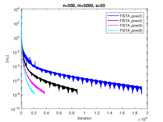
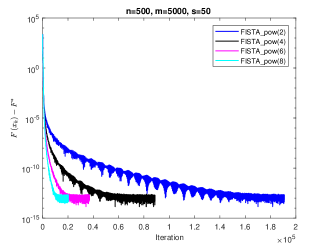
Considering Corollary 3.3. We know that in theory, the rate of convergence of IFB with in Case 2 should improve constantly as increasing. In the Fig.1, we test four choices of which is and to show the same result in experiments as in theory. Denote that the IFB with is called as “FISTA_pow(r)”. Here we set And the constant stepsize is
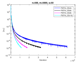
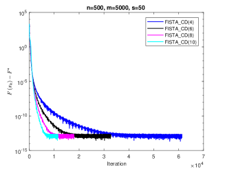
In Corollary 3.11, we show that the convergence rate of corresponding IFB greatly related to the value of In the Fig.2, we test four choices of which is and to verify our theoretical results. Set
Now, we perform numerical experiments to study the IFB with five choices of Notice that the IFBs with discussed in Case 1 and Case 3 enjoy the rates of convergence better than any order of convergence rate, and in the end of last section, we emphasize that these two IFBs should achieve almost the same numerical experiments if we set the related parameters as and Hence, we consider the following algorithms:
1) FISTA;
2) FISTA_CD with ;
3) FISTA_pow(8), i.e., the IFB with .
4) FISTA_pow(0.5), i.e., the IFB with .
5) FISTA_exp, i.e., the IFB with And set
Set
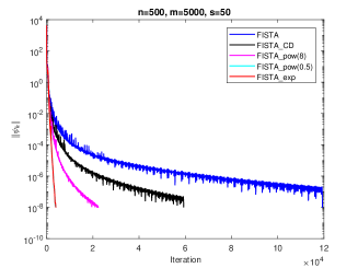
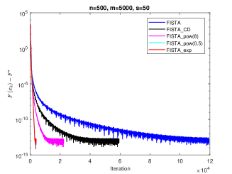
Our computational results are presented in Fig.3. We see that FISTA_exp and FISTA_pow(0.5) cost many fewer steps than FISTA_CD and FISTA, and faster than FISTA_pow(8). This results are same as the theoretical analyses in Section 3. And we see that the two lines of FISTA_exp and FISTA_pow(0.5) almost coincide, here, we give the detail number of iterations: for FISTA_exp, it’s number of iteration is 3948, and for FISTA_pow(0.5), it’s number of iteration is 3964, which confirms our theoretical analysis.
Sparse Logistic Regression. We also consider the sparse logistic regression with the regularized, that is
| (29) |
where Define and It satisfies the local error bound condition since the third example in Introduction with and Set We take three datasets “w4a”, “a9a” and “sonar” from LIBSVM (see, Chang & Lin, 2011). And the computational results relative to the number of iterations are reported in following Table 1.
| FISTA | FISTA_CD | FISTA_pow(8) | FISTA_pow(0.5) | FISTA_exp | |
|---|---|---|---|---|---|
| “ w4a ” | 1147 | 760 | 544 | 510 | 548 |
| “ a9a ” | 2049 | 1289 | 757 | 623 | 714 |
| “ sonar ” | 8405 | 3406 | 1586 | 922 | 980 |
We see from Table 1 that FISTA_exp, FISTA_pow(0.5) and FISTA_pow(8) outperform FISTA and FISTA_CD and the numerical results are consistent with the theoretical ones.
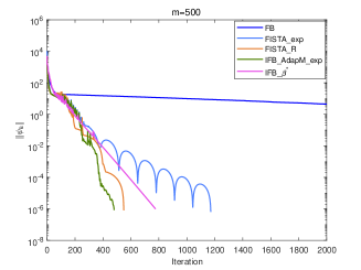
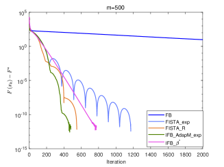
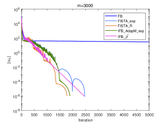
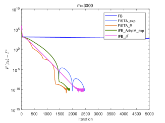
Strong convex quadratic programming with simplex constraints.
where is a symmetric positive definite matrix generated by where with i.i.d. standard Gaussian entries and chosen uniformly at random from . The vector is generated with i.i.d. standard Gaussian entries. Set = ones(m,1) and = -ones(m,1). Notice that with and and Here, we terminate the algorithms once
Now we perform numerical experiments with (1) Forward-Backward method without inertial (FB); (2) FISTA with fixed and adaptive restart schemes (FISTA_R); (3) IFB with (IFB_); (4) FISTA_exp; (5) Algorithm 2 (Gradient scheme) with (IFB_AdapM_exp).
According to Corollary 3.1, we know that sublinearly convergence rate for the sequences and generated by algorithms FISTA_exp and IFB_AdapM_exp, which slower than -linear convergence for algorithms FB, FISTA_R and IFB_ from a theoretical point of view. However, we can see from Fig.4 and Fig.5 that IFB_AdapM_exp always has better performance than FISTA_exp and sometimes, IFB_AdapM_exp performs better than other four algorithms and FISTA_exp performs similar with IFB_ but don’t require the strong convex parameter. Consequently, although the linear convergence rate is not reached, FISTA_exp and IFB_AdapM_exp still have good numerical performances, and this adaptive modification scheme can significantly improve the convergence speed of IFB.
6 Conclusion
In this paper, under the local error bound condition, we study the convergence results of IFBs with a class of abstract satisfying the assumption for solving the problem (). We use a new method called “comparison method” to discuss the improved convergence rates of function values and sublinear rates of convergence of iterates generated by the IFBs with six choices of In particular, we show that, under the local error bound condition, the strong convergence of iterates generated by the original FISTA can be established, the convergence rate of FISTA_CD is actually related to the value of and the sublinear convergence rates for both of function values and iterates generated by IFBs with in Case 1 and Case 3 can achieve for any positive integer Specifically, our results still hold for IFBs with an adaptive modification scheme.
Acknowledgements
The work was supported by the National Natural Science Foundation of China (No.11901561), the Natural Science Foundation of Guangxi (No.2018GXNSFBA281180) and the Postdoctoral Fund Project of China (Grant No.2019M660833).
References
- Attouch & Peypouquet (2016) Attouch, H. & Peypouquet, J. (2016) The rate of convergence of Nesterov’s accelerated forwardbackward method is actually faster than . SIAM J. Optim., 26, 1824–1834.
- Attouch & Cabot (2018) Attouch, H. & Cabot, A. (2018) Convergence rates of inertial forward-backward algorithms. SIAM J. Optim., 28, 849–874.
- Apidopoulos & Aujol (2020) Apidopoulos, V., Aujol, J. & Dossal, C. (2020) Convergence rate of inertial Forward-Backward algorithm beyond Nesterov’s rule. Math. Program., 180, 137–156.
- Beck & Teboulle (2009) Beck, A. & Teboulle, M. (2009) A fast iterative shrinkage-thresholding algorithm for linear inverse problems. SIAM J. Imaging Sci., 2, 183–202.
- Chambolle & Dossal (2015) Chambolle, A. & Dossal, C. (2015) On the convergence of the iterates of the “fast iterative shrinkage-thresholding algorithm. J. Optim. Theory Appl., 166, 968–982.
- Chambolle & Pock (2016) Chambolle, A. & Pock, T. (2015) An introduction to continuous optimization for imaging. Acta Numerica., 25, 161–319.
- Chang & Lin (2011) Chang, C. C. & Lin, C. J. (2011) LIBSVM: a library for support vector machines. ACM. Trans. Intell. Syst. Technol., 2, 1–27.
- Calatroni & Chambolle (2019) Calatroni, L. & Chambolle, A. (2019) Backtracking strategies for accelerated descent methods with smooth composite objectives. SIAM J. Optim., 29, 1772–1798.
- Donghwan & Jeffrey (2018) Donghwan, K. & Jeffrey, A. F. (2018) Another look at the fast iterative shrinkage/thresholding algorithm (FISTA). SIAM J. Optim., 28, 223–250.
- Hai (2020) Hai, T. N.. (2020) Error bounds and stability of the projection method for strongly pseudomonotone equilibrium problems. Int. J. Comput. Math., also available online from https://doi.org/10.1080/00207160.2019.1711374.html.
- Johnstone & Moulin (2017) Johnstone, P. R. & Moulin, P. (2017) Local and global convergence of a general inertial proximal splitting scheme for minimizing composite functions. Comput. Optim. Appl., 67, 259–292.
- Luo & Tseng (1992) Luo, Z. & Tseng, P. (1992) On the linear convergence of descent methods for convex essentially smooth minimization. SIAM J. Control Optim., 30, 408–425.
- Luo & Tseng (1992a) Luo, Z. & Tseng, P. (1992a) Error bound and convergence analysis of matrix splitting algorithms for the affine variational inequality problem. SIAM J. Optim., 2, 43-54.
- Luo & Tseng (1993) Luo, Z. & Tseng, P. (1993) On the convergence rate of dual ascent methods for linearly constrained convex minimization. Math. Oper. Res., 18, 846-867.
- Moudafi & Oliny (2003) Moudafi, A. & Oliny, M. (2003) Convergence of a splitting inertial proximal method for monotone operators. J. Comput. Appl. Math., 155, 447–454.
- Mridula & Shukla (2020) Mridula, V. & Shukla, K. K. (2020) Convergence analysis of accelerated proximal extra-gradient method with applications. Neurocomputing., 388, 288–300.
- Necoara & Nesterov (2019) Necoara, I., Nesterov, Y. & Glineur, F. (2019) Linear convergence of first order methods for non-strongly convex optimization. Math. Program., 175, 69–107.
- Nesterov (2019) Nesterov, Y. (2019) A method for solving the convex programming problem with convergence rate . Dokl. Akad. Nauk SSSR., 269, 543–547.
- Nesterov (2013) Nesterov, Y. (2013) Gradient methods for minimizing composite functions. Math. Program., 140, 125–161.
- O’Donoghue & Candès (2015) O’Donoghue, B. & Candès, E. (2015) Adaptive restart for accelerated gradient schemes. Dokl. Akad. Nauk SSSR., 15, 715–732.
- Pang (1987) Pang, J. S. (1987) A posteriori error bounds for the linearly-constrained variational inequality problem. Math. Oper. Res., 12, 474–484.
- Su & Boyd (2016) Su, W., Boyd, S. & Candès, E. J. (2016) A differential equation for modeling Nesterov’s accelerated gradient method: Theory and insights. J. Mach. Learn. Res., 17, 1–43.
- Tseng & Yun (2009) Tseng, P. & Yun, S. (2009) A coordinate gradient descent method for nonsmooth separable minimization. Math. Program., 117, 387–423.
- Tseng & Yun (2010) Tseng, P. & Yun, S. (2010) A coordinate gradient descent method for linearly constrained smooth optimization and support vector machines training. Comput Optim Appl., 47, 179–206.
- Tseng (2010) Tseng, P. (2010) Approximation accuracy, gradient methods, and error bound for structured convex optimization. Math. Program., 125, 263–295.
- Tao & Boley (2016) Tao, S. Z., Boley, D. & Zhang, S. Z. (2016) Local linear convergence of ISTA and FISTA on the LASSO problem. SIAM J. Optim., 26, 313–336.
- Villa & Salzo (2013) Villa, S., Salzo, S., Baldassarre, L. & Verri, A. (2013) Accelerated and Inexact Forward-Backward Algorithms. SIAM J. Optim., 23, 1607–1633.
- Wen & Chen (2017) Wen, B., Chen, X. J., & Pong, T. K. (2017) Linear convergence of proximal gradient algorithm with extrapolation for a class of nonconvex nonsmooth minimization problemsLinear convergence of proximal gradient algorithm with extrapolation for a class of nonconvex nonsmooth minimization problems. SIAM J. Optim., 27, 124–145.
- Xiao & Zhang (2013) Xiao, L. & Zhang, T. (2013) A Proximal-gradient homotopy method for the sparse least-squares problem. SIAM J. Optim., 23, 1062–1091.
- Zhou & So (2017) Zhou, Z. & So, A. M. (2017) A unified approach to error bounds for structured convex optimization problems. Math. Program., 165, 689–728.
- Nesterov (2003) Nesterov, Y. (2003) Introductory lectures on convex optimization: A basic course. Springer Science & Business Media.
Appendix A Proof of Lemma 2.4
Proof A.1.
Assume by contradiction that Notice that since that is a nonnegative sequence. Then, there exists a subsequence such that By the condition we have then, combining with the fact that from Remark 3, we deduce that
which leads to a contradiction that Hence,
Further, by the condition we get Combining with and we obtain that Since that is a nonnegative subsequence, we have which leads to the result that