This paper was converted on www.awesomepapers.org from LaTeX by an anonymous user.
Want to know more? Visit the Converter page.

Convergence Rate of LQG Mean Field Games with Common Noise

Jiamin Jian Qingshuo Song qsong@wpi.edu Jiaxuan Ye
Abstract

This paper focuses on exploring the convergence properties of a generic player’s trajectory and empirical measures in an NN-player Linear-Quadratic-Gaussian Nash game, where Brownian motion serves as the common noise. The study establishes three distinct convergence rates concerning the representative player and empirical measure. To investigate the convergence, the methodology relies on a specific decomposition of the equilibrium path in the NN-player game and utilizes the associated Mean Field Game framework.

1 Introduction

Mean Field Game (MFG) theory was introduced by Lasry and Lions in their seminal paper ([19]), and by Huang, Caines, and Malhame ([15, 13, 14, 12]). It aims to provide a framework for studying the asymptotic behavior of NN-player differential games being invariant under the reshuffling of the players’ indices. For a comprehensive overview of recent advancements and relevant applications of MFG theory, it is recommended to refer to the two-volume book by Carmona and Delarue ([4, 5]) published in 2018 and the references provided therein.

Mean Field Games (MFG) have become widely accepted as an approximation for NN-player games, particularly when the number of players, NN, is large enough. A fundamental question that arises in this context concerns the convergence rate of this approximation. Convergence can be analyzed from different perspectives, such as convergence in value, the trajectory followed by the representative player, or the behavior of the mean field term. Each of these perspectives offers valuable insights into the behavior and characteristics of the MFG approximation. Furthermore, they raise a variety of intriguing questions within this context.

To be more concrete, we examine the behavior of the triangular array X^t(N)=(X^it(N):1iN)\hat{X}_{t}^{(N)}=(\hat{X}_{it}^{(N)}:1\leq i\leq N) as NN\to\infty, where X^it(N)\hat{X}_{it}^{(N)} represents the equilibrium state of the ii-th player at time tt in the NN-player game, defined within the probability space (Ω(N),(N),𝔽(N),(N))\left(\Omega^{(N)},\mathcal{F}^{(N)},\mathbb{F}^{(N)},\mathbb{P}^{(N)}\right). Additionally, we denote X^t\hat{X}_{t} as the equilibrium path at time tt derived from the associated MFG, defined in the probability space (Ω,,𝔽,)(\Omega,\mathcal{F},\mathbb{F},\mathbb{P}).

Considering the identical but not independent distribution (X^it(N))\mathcal{L}(\hat{X}_{it}^{(N)}), the first question pertains to the convergence of X^1t(N)\hat{X}_{1t}^{(N)}, which represents the generic path. It can be framed as follows:

  • (Q1)

    The 𝕎p\mathbb{W}_{p}-convergence rate of the representative equilibrium path,

    𝕎p((X^1t(N)),(X^t))=O(N?).\mathbb{W}_{p}\left(\mathcal{L}\left(\hat{X}_{1t}^{(N)}\right),\mathcal{L}\left(\hat{X}_{t}\right)\right)=O\left(N^{-?}\right).

Here, 𝕎p\mathbb{W}_{p} denotes the pp-Wasserstein metric.

The existing literature extensively explores the convergence rate in this context. For (Q1), Theorem 2.4.9 of the monograph [3] establishes a convergence rate of O(N1/2)O(N^{-1/2}) using the 𝕎1\mathbb{W}_{1} metric. More recently, [17] addresses (Q1) by introducing displacement monotonicity and controlled common noise, and Theorem 2.23 applies the maximum principle of forward-backward propagation of chaos to achieve the same convergence rate. Within the LQG framework, [18] also provides a convergence rate of 1/21/2 for the representative player.

The second question pertains to the convergence of the mean-field term, which is equivalent to the convergence of the empirical measure ρ(X^t(N))=1Ni=1NδX^it(N)\rho(\hat{X}_{t}^{(N)})=\frac{1}{N}\sum_{i=1}^{N}\delta_{\hat{X}_{it}^{(N)}} of NN players. Given the Brownian motion, denoted as W~t\tilde{W}_{t}, to be the common noise, the problem lies in determining the rate of convergence of the empirical measures to the MFG equilibrium measure

m^t=(X^t|tW~),t(0,T].\hat{m}_{t}=\mathcal{L}\left(\left.\hat{X}_{t}\right|{\mathcal{F}}_{t}^{\tilde{W}}\right),\quad\forall t\in(0,T].

Thus, the second question can be stated as follows:

  • (Q2)

    The 𝕎p\mathbb{W}_{p}-convergence rate of empirical measures in LpL^{p} sense,

    (𝔼[𝕎pp(ρ(X^t(N)),(X^t|tW~))])1p=O(N?).\left(\mathbb{E}\left[\mathbb{W}_{p}^{p}\left(\rho\left(\hat{X}_{t}^{(N)}\right),\mathcal{L}\left(\left.\hat{X}_{t}\right|{\mathcal{F}}_{t}^{\tilde{W}}\right)\right)\right]\right)^{\frac{1}{p}}=O\left(N^{-?}\right).

As for (Q2), Theorem 3.1 of [8] provides an answer, stating that the empirical measures exhibit a convergence rate of O(N1/(2p))O(N^{-1/(2p)}) in the 𝕎p\mathbb{W}_{p} distance for p[1,2]p\in[1,2]. In [8], they also explore a related question that is both similar and more intriguing, which concerns the uniform 𝕎p\mathbb{W}_{p}-convergence rate:

  • (Q3)

    The tt-uniform 𝕎p\mathbb{W}_{p}-convergence rate of empirical measures in LpL^{p} sense,

    (𝔼[supt[0,T]𝕎pp(ρ(X^t(N)),(X^t|tW~))])1p=O(N?).\left(\mathbb{E}\left[\sup_{t\in[0,T]}\mathbb{W}_{p}^{p}\left(\rho\left(\hat{X}_{t}^{(N)}\right),\mathcal{L}\left(\left.\hat{X}_{t}\right|{\mathcal{F}}_{t}^{\tilde{W}}\right)\right)\right]\right)^{\frac{1}{p}}=O\left(N^{-?}\right).

The answer provided by Theorem 3.1 in [8] reveals that the uniform convergence rate, as formulated in (Q3), is considerably slower compared to the convergence rate mentioned in (Q2). Specifically, the convergence rate for (Q3) is O(N1/(d+8))O\left(N^{-1/(d+8)}\right) when p=2p=2, where dd represents the dimension of the state space.

In our paper, we specifically focus on a class of one-dimensional Linear-Quadratic-Gaussian (LQG) Mean Field Nash Games with Brownian motion as the common noise. It is important to note that the assumptions made in the aforementioned papers except [18] only account for linear growth in the state and control elements for the running cost, thus excluding the consideration of LQG. It is also noted that differences between [18] and the current paper lie in various aspects: (1) The problem setting in our paper considers Brownian motion as the common noise, whereas [18] employs a Markov chain. This discrepancy leads to significant differences in the subsequent analysis; (2) The work in [18] does not address the questions posed in (Q2) and (Q3).

Our main contribution is the establishment of the convergence rate of all three questions in the above in LQG framework. Firstly, the paper establishes that the convergence rate of the pp-Wasserstein metric for the distribution of the representative player is O(N1/2)O(N^{-1/2}) for p[1,2]p\in[1,2]. Secondly, it demonstrates that the convergence rate of the pp-Wasserstein metric for the empirical measure in the LpL^{p} sense is O(N1/(2p))O(N^{-1/(2p)}) for p[1,2]p\in[1,2]. Lastly, the paper shows that the convergence rate of the uniform pp-Wasserstein metric for the empirical measure in the LpL^{p} sense is O(N1/(2p))O(N^{-1/(2p)}) for p(1,2]p\in(1,2], and O(N1/2ln(N))O(N^{-1/2}\ln(N)) for p=1p=1.

It is worth noting that the convergence rates obtained for (Q1) and (Q2) in the LQG framework align with the results found in existing literature, albeit under different conditions. Additionally, it is revealed that the uniform convergence rate of (Q3) may be slower than that of (Q2), which is consistent with the observations made by [8] from a similar perspective. Interestingly, when considering the specific case where p=2p=2 and d=1d=1, the uniform convergence rate of (Q3) is established as O(N1/9)O(N^{-1/9}) according to [8], while it is determined to be O(N1/4)O(N^{-1/4}) within our framework that incorporates the LQG structure.

Regarding (Q2), if the states (X^it(N):1iN)(\hat{X}_{it}^{(N)}:1\leq i\leq N) were independent, the convergence rate could be determined as 1/(2p)1/(2p) based on Theorem 1 of [10] and Theorem 5.8 of [4], which provide convergence rates for empirical measures of independent and identically distributed sequences. However, in the mean-field game, the states X^it(N)\hat{X}_{it}^{(N)} are not independent of each other, despite having identical distributions. The correlation is introduced mainly by two factors: One is the system coupling arising from the mean-field term and the other is the common noise. Consequently, determining the convergence rate requires understanding the contributions of these two factors to the correlation among players.

In our proof, we rely on a specific decomposition (refer to Lemma 6 and the proof of the main theorem) of the underlying states. This decomposition reveals that the states can be expressed as a sum of a weakly correlated triangular array and a common noise. By analyzing the behavior of these components, we can address the correlation and establish the convergence rate.

Additionally, it is worth mentioning that a similar technique of dimension reduction in NN-player LQG games have been previously utilized in [16] and related papers to establish decentralized Nash equilibria and the convergence rate in terms of value functions.

The remainder of the paper is organized as follows: Section 2 outlines the problem setup and presents the main result. The proof of the main result, which relies on two propositions, is provided in Section 3. We establish the proof for these two propositions in Section 4 and Section 5. Some lemmas are given in the Appendix.

2 Problem setup and main results

2.1 The formulation of equilibrium in Mean Field Game

In this section, we present the formulation of the Mean Field Game in the sample space Ω\Omega.

Let T>0T>0 be a given time horizon. We assume that W={Wt}t0W=\{W_{t}\}_{t\geq 0} is a standard Brownian motion constructed on the probability space (Ω¯,¯=¯T,¯,𝔽¯={¯t}t0)(\bar{\Omega},\bar{\mathcal{F}}=\bar{\mathcal{F}}_{T},\bar{\mathbb{P}},\bar{\mathbb{F}}=\{\bar{\mathcal{F}}_{t}\}_{t\geq 0}). Similarly, the process W~={W~t}t0\tilde{W}=\{\tilde{W}_{t}\}_{t\geq 0} is a standard Brownian motion constructed on the probability space (Ω~,~=~T,~,𝔽~={~t}t0)(\tilde{\Omega},\tilde{\mathcal{F}}=\tilde{\mathcal{F}}_{T},\tilde{\mathbb{P}},\tilde{\mathbb{F}}=\{\tilde{\mathcal{F}}_{t}\}_{t\geq 0}). We define the product structure as follows:

Ω=Ω¯×Ω~,,𝔽={t}t0,,\Omega=\bar{\Omega}\times\tilde{\Omega},\quad\mathcal{F},\quad\mathbb{F}=\{\mathcal{F}_{t}\}_{t\geq 0},\quad\mathbb{P},

where (,)(\mathcal{F},\mathbb{P}) is the completion of (¯~,¯~)(\bar{\mathcal{F}}\otimes\tilde{\mathcal{F}},\bar{\mathbb{P}}\otimes\tilde{\mathbb{P}}) and 𝔽\mathbb{F} is the complete and right continuous augmentation of {¯t~t}t0\{\bar{\mathcal{F}}_{t}\otimes\tilde{\mathcal{F}}_{t}\}_{t\geq 0}.

Note that, WW and W~\tilde{W} are two Brownian motions from separate sample spaces Ω¯\bar{\Omega} and Ω~\tilde{\Omega}, they are independent of each other in their product space Ω\Omega. In our manuscript, WW is called individual or idiosyncratic noise, and W~\tilde{W} is called common noise, see their different roles in the problem formulation later defined via fixed point condition (4). To proceed, we denote by Lp:=Lp(Ω,)L^{p}:=L^{p}(\Omega,\mathbb{P}) the set of random variables XX on (Ω,,)(\Omega,\mathcal{F},\mathbb{P}) with finite pp-th moment with norm Xp=(𝔼[|X|p])1/p\|X\|_{p}=(\mathbb{E}\left[|X|^{p}\right])^{1/p} and by L𝔽p:=L𝔽p(Ω×[0,T])L_{\mathbb{F}}^{p}:=L_{\mathbb{F}}^{p}(\Omega\times[0,T]) the space of all \mathbb{R} valued 𝔽\mathbb{F}-progressively measurable random processes α\alpha such that

𝔼[0T|αt|p𝑑t]<.\mathbb{E}\left[\int_{0}^{T}|\alpha_{t}|^{p}dt\right]<\infty.

Let 𝒫p()\mathcal{P}_{p}(\mathbb{R}) denote the Wasserstein space of probability measures μ\mu on \mathbb{R} satisfying xp𝑑μ(x)<\int_{\mathbb{R}}x^{p}d\mu(x)<\infty endowed with pp-Wasserstein metric 𝕎p(,)\mathbb{W}_{p}(\cdot,\cdot) defined by

𝕎p(μ,ν)=infπΠ(μ,ν)(×|xy|p𝑑π(x,y))1p,\mathbb{W}_{p}(\mu,\nu)=\inf_{\pi\in\Pi(\mu,\nu)}\left(\int_{\mathbb{R}\times\mathbb{R}}|x-y|^{p}d\pi(x,y)\right)^{\frac{1}{p}},

where Π(μ,ν)\Pi(\mu,\nu) is the collection of all probability measures on ×\mathbb{R}\times\mathbb{R} with its marginals agreeing with μ\mu and ν\nu.

Let X0L2X_{0}\in L^{2} be a random variable that is independent with WW and W~\tilde{W}. For any control αL𝔽2\alpha\in L^{2}_{\mathbb{F}}, consider the state X={Xt}t0X=\{X_{t}\}_{t\geq 0} of the generic player is governed by a stochastic differential equation (SDE)

dXt=αtdt+dWt+dW~tdX_{t}=\alpha_{t}dt+dW_{t}+d\tilde{W}_{t} (1)

with the initial value X0X_{0}, where the underlying process X:[0,T]×ΩX:[0,T]\times\Omega\mapsto\mathbb{R}. Given a random measure flow m:(0,T]×Ω𝒫2()m:(0,T]\times\Omega\mapsto\mathcal{P}_{2}(\mathbb{R}), the generic player wants to minimize the expected accumulated cost on [0,T][0,T]:

J(x,α)=𝔼[0T(12αs2+F(Xs,ms))ds|X0=x]\begin{array}[]{ll}J(x,\alpha)=\displaystyle\mathbb{E}\left[\left.\int_{0}^{T}\left(\frac{1}{2}\alpha_{s}^{2}+F(X_{s},m_{s})\right)\,ds\right\rvert X_{0}=x\right]\end{array} (2)

with some given cost function F:×𝒫2()F:\mathbb{R}\times\mathcal{P}_{2}(\mathbb{R})\mapsto\mathbb{R}.

The objective of the control problem for the generic player is to find its optimal control α^𝒜:=L𝔽4\hat{\alpha}\in\mathcal{A}:=L^{4}_{\mathbb{F}} to minimize the total cost, i.e.,

V[m](x)=J[m](x,α^)J[m](x,α),α𝒜.V[m](x)=J[m](x,\hat{\alpha})\leq J[m](x,\alpha),\quad\forall\alpha\in\mathcal{A}. (3)

Associated to the optimal control α^\hat{\alpha}, we denote the optimal path by X^={X^t}t0\hat{X}=\{\hat{X}_{t}\}_{t\geq 0}.

Next, to introduce the MFG Nash equilibrium, it is useful to emphasize the dependence of the optimal path and optimal control of the generic player, as well as its associated value, on the underlying measure flow mm. These quantities are denoted as X^t[m]\hat{X}_{t}[m], α^t[m]\hat{\alpha}_{t}[m], J[m]J[m], and V[m]V[m], respectively.

We now present the definitions of the equilibrium measure, equilibrium path, and equilibrium control. Please also refer to page 127 of [5] for a general setup with a common noise.

Definition 1.

Given an initial distribution (X0)=m0𝒫2()\mathcal{L}(X_{0})=m_{0}\in\mathcal{P}_{2}(\mathbb{R}), a random measure flow m^=m^(m0)\hat{m}=\hat{m}(m_{0}) is said to be an MFG equilibrium measure if it satisfies the fixed point condition

m^t=(X^t[m^]|~t),0<tT, almost surely in .\hat{m}_{t}=\mathcal{L}\left(\left.\hat{X}_{t}[\hat{m}]\right\rvert\tilde{\mathcal{F}}_{t}\right),\ \forall 0<t\leq T,\ \hbox{ almost surely in }\mathbb{P}. (4)

The path X^\hat{X} and the control α^\hat{\alpha} associated with m^\hat{m} are called the MFG equilibrium path and equilibrium control, respectively.

Refer to caption
Figure 1: The MFG diagram.

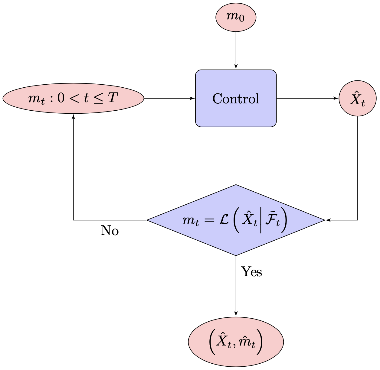
The flowchart of the MFG diagram is given in Figure 1. It is noted from the optimality condition (3) and the fixed point condition (4) that

J[m^](x,α^)J[m^](x,α),αJ[\hat{m}](x,\hat{\alpha})\leq J[\hat{m}](x,\alpha),\quad\forall\alpha

holds for the equilibrium measure m^\hat{m} and its associated equilibrium control α^\hat{\alpha}, while it is not

J[m^](x,α^)J[m](x,α),α,m.J[\hat{m}](x,\hat{\alpha})\leq J[m](x,\alpha),\quad\forall\alpha,m.

Otherwise, this problem turns into a McKean-Vlasov control problem, which is essentially different from the current Mean Field Games setup. Readers refer to [7, 6] to see the analysis of this different model as well as some discussion of the differences between these two problems.

2.2 The formulation of Nash equilibrium in NN-player game

In this subsection, we set up NN-player game and define the Nash equilibrium of NN-player game in the sample space Ω(N)\Omega^{(N)}. Firstly, let W(N)=(Wi(N):i=1,2,,N)W^{(N)}=(W^{(N)}_{i}:i=1,2,\dots,N) be an NN-dimensional standard Brownian motion constructed on the space (Ω¯(N),¯(N),¯(N),𝔽¯(N)={¯t(N)}t0)(\bar{\Omega}^{(N)},\bar{\mathcal{F}}^{(N)},\bar{\mathbb{P}}^{(N)},\bar{\mathbb{F}}^{(N)}=\{\bar{\mathcal{F}}^{(N)}_{t}\}_{t\geq 0}) and W~={W~t}t0\tilde{W}=\{\tilde{W}_{t}\}_{t\geq 0} be the common noise in MFG defined in Section 2.1 on (Ω~,~,~)(\tilde{\Omega},\tilde{\mathcal{F}},\tilde{\mathbb{P}}). The probability space for the NN-player game is (Ω(N),(N),𝔽(N),(N))\left(\Omega^{(N)},\mathcal{F}^{(N)},\mathbb{F}^{(N)},\mathbb{P}^{(N)}\right), which is constructed via the product structure with

Ω(N)=Ω¯(N)×Ω~,(N),𝔽(N)={t(N)}t0,(N).\Omega^{(N)}=\bar{\Omega}^{(N)}\times\tilde{\Omega},\quad\mathcal{F}^{(N)},\quad\mathbb{F}^{(N)}=\left\{\mathcal{F}^{(N)}_{t}\right\}_{t\geq 0},\quad\mathbb{P}^{(N)}.

where ((N),(N))(\mathcal{F}^{(N)},\mathbb{P}^{(N)}) is the completion of (¯(N)~,¯(N)~)(\bar{\mathcal{F}}^{(N)}\otimes\tilde{\mathcal{F}},\bar{\mathbb{P}}^{(N)}\otimes\tilde{\mathbb{P}}) and 𝔽(N)\mathbb{F}^{(N)} is the complete and right continuous augmentation of {¯t(N)~t}t0\{\bar{\mathcal{F}}_{t}^{(N)}\otimes\tilde{\mathcal{F}}_{t}\}_{t\geq 0}.

Consider a stochastic dynamic game with NN players, where each player i{1,2,,N}i\in\{1,2,\dots,N\} controls a state process Xi(N)={Xit(N)}t0X_{i}^{(N)}=\{X_{it}^{(N)}\}_{t\geq 0} in \mathbb{R} given by

dXit(N)=αit(N)dt+dWit(N)+dW~t,Xi0(N)=xi(N)dX_{it}^{(N)}=\alpha_{it}^{(N)}dt+dW_{it}^{(N)}+d\tilde{W}_{t},\quad X_{i0}^{(N)}=x^{(N)}_{i} (5)

with a control αi(N)\alpha_{i}^{(N)} in an admissible set 𝒜(N):=L𝔽(N)4\mathcal{A}^{(N)}:=L^{4}_{\mathbb{F}^{(N)}} and random initial state xi(N)x^{(N)}_{i}.

Given the strategies αi(N)=(α1(N),,αi1(N),αi+1(N),,αN(N))\alpha_{-i}^{(N)}=(\alpha_{1}^{(N)},\dots,\alpha_{i-1}^{(N)},\alpha_{i+1}^{(N)},\dots,\alpha_{N}^{(N)}) from other players, the objective of player ii is to select a control αi(N)𝒜(N)\alpha_{i}^{(N)}\in\mathcal{A}^{(N)} to minimize her expected total cost given by

JiN(x(N),αi(N);αi(N))\displaystyle J_{i}^{N}\left(x^{(N)},\alpha_{i}^{(N)};\alpha_{-i}^{(N)}\right) =𝔼[0T(12(αit(N))2+F(Xit(N),ρ(Xt(N))))dt|X0(N)=x(N)],\displaystyle=\mathbb{E}\left[\left.\int_{0}^{T}\left(\frac{1}{2}\left(\alpha_{it}^{(N)}\right)^{2}+F\left(X_{it}^{(N)},\rho\left(X_{t}^{(N)}\right)\right)\right)dt\right\rvert X_{0}^{(N)}=x^{(N)}\right], (6)

where x(N)=(x1(N),x2(N),,xN(N))x^{(N)}=(x_{1}^{(N)},x_{2}^{(N)},\dots,x_{N}^{(N)}) is a N\mathbb{R}^{N}-valued random vector in Ω(N)\Omega^{(N)} to denote the initial state for NN players, and

ρ(x(N))=1Ni=1Nδxi(N)\rho\left(x^{(N)}\right)=\frac{1}{N}\sum_{i=1}^{N}\delta_{x_{i}^{(N)}}

is the empirical measure of the vector x(N)x^{(N)} with Dirac measure δ\delta. We use the notation α(N):=(αi(N),αi(N))=(α1(N),α2(N),,αN(N))\alpha^{(N)}:=(\alpha_{i}^{(N)},\alpha_{-i}^{(N)})=(\alpha_{1}^{(N)},\alpha_{2}^{(N)},\ldots,\alpha_{N}^{(N)}) to denote the control from NN players as a whole. Next, we give the equilibrium value function and equilibrium path in the sense of the Nash game.

Definition 2.
  1. 1.

    The value function of player ii for i=1,2,,Ni=1,2,\ldots,N of the Nash game is defined by VN=(ViN:i=1,2,,N)V^{N}=(V^{N}_{i}:i=1,2,\ldots,N) satisfying the equilibrium condition

    ViN(x(N)):=JiN(x(N),α^i(N);α^i(N))JiN(x(N),αi(N);α^i(N)),αi(N)𝒜(N).V_{i}^{N}\left(x^{(N)}\right):=J_{i}^{N}\left(x^{(N)},\hat{\alpha}_{i}^{(N)};\hat{\alpha}_{-i}^{(N)}\right)\leq J_{i}^{N}\left(x^{(N)},\alpha_{i}^{(N)};\hat{\alpha}_{-i}^{(N)}\right),\quad\forall\alpha_{i}^{(N)}\in\mathcal{A}^{(N)}. (7)
  2. 2.

    The equilibrium path of the NN-player game is the NN-dimensional random path X^t(N)=(X^1t(N),X^2t(N),,X^Nt(N))\hat{X}_{t}^{(N)}=(\hat{X}_{1t}^{(N)},\hat{X}_{2t}^{(N)},\ldots,\hat{X}_{Nt}^{(N)}) driven by (5) associated to the control α^t(N)\hat{\alpha}_{t}^{(N)} satisfying the equilibrium condition of (7).

2.3 Main result

We consider three convergence questions on NN-player game defined in Ω(N)\Omega^{(N)}: The first one is the convergence of the representative path X^it(N)\hat{X}_{it}^{(N)}, the second one is the convergence of the empirical measure ρ(X^t(N))\rho(\hat{X}_{t}^{(N)}), while the last one is the tt-uniform convergence of the empirical measure ρ(X^t(N))\rho(\hat{X}_{t}^{(N)}). To be precise, we shall assume the following throughout the paper:

Assumption 1.
  • 𝔼[|X0|q]<\mathbb{E}[|X_{0}|^{q}]<\infty for some q>4q>4.

  • The initials Xi0(N)X_{i0}^{(N)} of the NN-player game is i.i.d. random variables in Ω(N)\Omega^{(N)} with the same distribution as (X0)\mathcal{L}(X_{0}) in the MFG.

Note that the equilibrium path X^t(N)=(X^it(N):i=1,2,,N)\hat{X}_{t}^{(N)}=(\hat{X}_{it}^{(N)}:i=1,2,\ldots,N) is a vector-valued stochastic process. Due to the Assumption 1, the game is invariant to index reshuffling of NN players and the elements in (X^it(N):i=1,2,,N)(\hat{X}_{it}^{(N)}:i=1,2,\ldots,N) have identical distributions, but they are not independent of each other.

So, the first question on the representative path is indeed about X^1t(N)\hat{X}_{1t}^{(N)} in Ω(N)\Omega^{(N)} and we are interested in how fast it converges to X^t\hat{X}_{t} in Ω\Omega in distribution:

  • (Q1)

    The 𝕎p\mathbb{W}_{p}-convergence rate of the representative equilibrium path,

    𝕎p((X^1t(N)),(X^t))=O(N?).\mathbb{W}_{p}\left(\mathcal{L}\left(\hat{X}_{1t}^{(N)}\right),\mathcal{L}\left(\hat{X}_{t}\right)\right)=O\left(N^{-?}\right).

The second question is about the convergence of the empirical measure ρ(X^t(N))\rho(\hat{X}_{t}^{(N)}) of the NN-player game defined by

ρ(X^t(N))=1Ni=1NδX^it(N).\rho\left(\hat{X}_{t}^{(N)}\right)=\frac{1}{N}\sum_{i=1}^{N}\delta_{\hat{X}_{it}^{(N)}}.

We are interested in how fast this converges to the MFG equilibrium measure given by

m^t=(X^t|~t),t(0,T].\hat{m}_{t}=\mathcal{L}\left(\left.\hat{X}_{t}\right|\tilde{\mathcal{F}}_{t}\right),\quad\forall t\in(0,T].
  • (Q2’)

    The 𝕎p\mathbb{W}_{p}-convergence rate of empirical measures,

    𝕎p(ρ(X^t(N)),(X^t|~t))=O(N?).\mathbb{W}_{p}\left(\rho\left(\hat{X}_{t}^{(N)}\right),\mathcal{L}\left(\left.\hat{X}_{t}\right|\tilde{\mathcal{F}}_{t}\right)\right)=O\left(N^{-?}\right).

Note that the left-hand side of the above equality is a random quantity and one shall be more precise about what the Big OO notation means in this context. Indeed, by the definition of the empirical measure, ρ(X^t(N))\rho(\hat{X}_{t}^{(N)}) is a random distribution measurable by σ\sigma-algebra generated by the random vector X^t(N)\hat{X}_{t}^{(N)}. On the other hand, (X^t|~t)\mathcal{L}(\hat{X}_{t}\rvert\tilde{\mathcal{F}}_{t}) is a random distribution measurable by the σ\sigma-algebra ~t\tilde{\mathcal{F}}_{t}. Therefore, from the construction of the product probability space Ω(N)\Omega^{(N)} in Section 2.2, both random distributions ρ(X^t(N))\rho(\hat{X}_{t}^{(N)}) and (X^t|~t)\mathcal{L}(\hat{X}_{t}\rvert\tilde{\mathcal{F}}_{t}) are measurable with respect to t(N)=¯t(N)~t\mathcal{F}^{(N)}_{t}=\bar{\mathcal{F}}_{t}^{(N)}\otimes\tilde{\mathcal{F}}_{t}. Consequently, 𝕎p(ρ(X^t(N)),(X^t|~t))\mathbb{W}_{p}(\rho(\hat{X}_{t}^{(N)}),\mathcal{L}(\hat{X}_{t}\rvert\tilde{\mathcal{F}}_{t})) is a random variable in the probability space (Ω(N),(N),(N))(\Omega^{(N)},\mathcal{F}^{(N)},\mathbb{P}^{(N)}) and we will focus on a version of (Q2’) in the LpL^{p} sense:

  • (Q2)

    The 𝕎p\mathbb{W}_{p}-convergence rate of empirical measures in LpL^{p} sense for each t[0,T]t\in[0,T],

    (𝔼[𝕎pp(ρ(X^t(N)),(X^t|~t))])1p=O(N?).\left(\mathbb{E}\left[\mathbb{W}_{p}^{p}\left(\rho\left(\hat{X}_{t}^{(N)}\right),\mathcal{L}\left(\left.\hat{X}_{t}\right|\tilde{\mathcal{F}}_{t}\right)\right)\right]\right)^{\frac{1}{p}}=O\left(N^{-?}\right).

In addition, we also study the following related question:

  • (Q3)

    The tt-uniform 𝕎p\mathbb{W}_{p}-convergence rate of empirical measures in LpL^{p} sense,

    (𝔼[sup0tT𝕎pp(ρ(X^t(N)),(X^t|~t))])1p=O(N?).\left(\mathbb{E}\left[\sup_{0\leq t\leq T}\mathbb{W}_{p}^{p}\left(\rho\left(\hat{X}_{t}^{(N)}\right),\mathcal{L}\left(\left.\hat{X}_{t}\right|\tilde{\mathcal{F}}_{t}\right)\right)\right]\right)^{\frac{1}{p}}=O\left(N^{-?}\right).

In this paper, we will study the above three questions (Q1), (Q2), and (Q3) in the framework of LQG structure with Brownian motion as a common noise with the following function FF in the cost functional (2).

Assumption 2.

Let the function F:×𝒫2()F:\mathbb{R}\times\mathcal{P}_{2}(\mathbb{R})\mapsto\mathbb{R} be given in the form of

F(x,m)=k(xz)2m(dz)=k(x22x[m]1+[m]2)F(x,m)=k\int_{\mathbb{R}}(x-z)^{2}m(dz)=k(x^{2}-2x[m]_{1}+[m]_{2}) (8)

for some k>0k>0, where [m]1,[m]2[m]_{1},[m]_{2} are the first and second moment of the measure mm.

The main result of this paper is presented below. Let us recall that qq denotes the parameter defined in Assumption 1.

Theorem 1.

Under Assumptions 1-2, for any p[1,2]p\in[1,2], we have

  1. 1.

    The 𝕎p\mathbb{W}_{p}-convergence rate of the representative equilibrium path is 1/21/2, i.e.,

    𝕎p((X^1t(N)),(X^t))=O(N12).\mathbb{W}_{p}\left(\mathcal{L}\left(\hat{X}_{1t}^{(N)}\right),\mathcal{L}\left(\hat{X}_{t}\right)\right)=O\left(N^{-\frac{1}{2}}\right).
  2. 2.

    The 𝕎p\mathbb{W}_{p}-convergence rate of empirical measures in LpL^{p} sense is

    𝔼[𝕎pp(ρ(X^t(N)),(X^t|~t))]=O(N12).\mathbb{E}\left[\mathbb{W}_{p}^{p}\left(\rho\left(\hat{X}_{t}^{(N)}\right),\mathcal{L}\left(\left.\hat{X}_{t}\right|\tilde{\mathcal{F}}_{t}\right)\right)\right]=O\left(N^{-\frac{1}{2}}\right).
  3. 3.

    The uniform 𝕎p\mathbb{W}_{p}-convergence rate of empirical measures in LpL^{p} sense is

    𝔼[sup0tT𝕎pp(ρ(X^t(N)),(X^t|~t))]={O(N12ln(N)), if p=1,O(N12), if 1<p2.\mathbb{E}\left[\sup_{0\leq t\leq T}\mathbb{W}_{p}^{p}\left(\rho\left(\hat{X}_{t}^{(N)}\right),\mathcal{L}\left(\left.\hat{X}_{t}\right|\tilde{\mathcal{F}}_{t}\right)\right)\right]=\begin{cases}O\left(N^{-\frac{1}{2}}\ln(N)\right),&\hbox{ if }p=1,\\ O\left(N^{-\frac{1}{2}}\right),&\hbox{ if }1<p\leq 2.\end{cases}

We would like to provide some additional remarks on our main result. Firstly, the cost function FF defined in (6) applies to the running cost for the ii-th player in the NN-player game, and it takes the form:

F(Xit(N),ρ(Xt(N)))=kNj=1N(Xit(N)Xjt(N))2.F\left(X_{it}^{(N)},\rho\left(X_{t}^{(N)}\right)\right)=\frac{k}{N}\sum_{j=1}^{N}\left(X_{it}^{(N)}-X_{jt}^{(N)}\right)^{2}. (9)

Interestingly, if k<0k<0, although FF does satisfy the Lasry-Lions monotonicity ([2]) as demonstrated in Appendix 6.1 of [18], there is no global solution for MFG due to the concavity in xx. On the contrary, when k>0k>0, FF satisfies the displacement monotonicity proposed in [11] as shown by the following derivation:

𝔼[(Fx(X1,(X1))Fx(X2,(X2)))(X1X2)]=2k(𝔼[(X1X2)2](𝔼[X1X2])2)0.\mathbb{E}\left[(F_{x}(X_{1},\mathcal{L}(X_{1}))-F_{x}(X_{2},\mathcal{L}(X_{2})))(X_{1}-X_{2})\right]=2k\left(\mathbb{E}\left[(X_{1}-X_{2})^{2}\right]-\left(\mathbb{E}[X_{1}-X_{2}]\right)^{2}\right)\geq 0.

3 Proof of the main result with two propositions

Our objective is to investigate the relations between (X^1t(N),X^2t(N),,X^Nt(N))(\hat{X}_{1t}^{(N)},\hat{X}_{2t}^{(N)},\ldots,\hat{X}_{Nt}^{(N)}) and X^t\hat{X}_{t} described in (Q1), (Q2), and (Q3). In this part, we will give the proof of Theorem 1 based on two propositions whose proof will be given later.

Proposition 1.

Under Assumptions 1-2, the MFG equilibrium path X^=X^[m^]\hat{X}=\hat{X}[\hat{m}] is given by

dX^t=2a(t)(X^tμ^t)dt+dWt+dW~t,X^0=X0,d\hat{X}_{t}=-2a(t)\left(\hat{X}_{t}-\hat{\mu}_{t}\right)dt+dW_{t}+d\tilde{W}_{t},\quad\hat{X}_{0}=X_{0}, (10)

where aa is the solution of

a(t)2a2(t)+k=0,a(T)=0,a^{\prime}(t)-2a^{2}(t)+k=0,\quad a(T)=0, (11)

and μ^\hat{\mu} is

μ^t:=𝔼[X^t|~t]=𝔼[X0]+W~t.\hat{\mu}_{t}:=\mathbb{E}\left[\left.\hat{X}_{t}\right|\tilde{\mathcal{F}}_{t}\right]=\mathbb{E}[X_{0}]+\tilde{W}_{t}.

Moreover, the equilibrium control follows

α^t=2a(t)(X^tμ^t).\hat{\alpha}_{t}=-2a(t)\left(\hat{X}_{t}-\hat{\mu}_{t}\right). (12)
Proposition 2.

Suppose Assumptions 1-2 hold. For the NN-player game, the path and the control of player ii under the equilibrium are given by

dX^it(N)=2aN(t)(X^it(N)1N1jiNX^jt(N))dt+dWit(N)+dW~t,d\hat{X}_{it}^{(N)}=-2a^{N}(t)\left(\hat{X}_{it}^{(N)}-\frac{1}{N-1}\sum_{j\neq i}^{N}\hat{X}_{jt}^{(N)}\right)dt+dW_{it}^{(N)}+d\tilde{W}_{t}, (13)

and

α^it(N)=2aN(t)(X^it(N)1N1jiNX^jt(N))\hat{\alpha}_{it}^{(N)}=-2a^{N}(t)\left(\hat{X}_{it}^{(N)}-\frac{1}{N-1}\sum_{j\neq i}^{N}\hat{X}_{jt}^{(N)}\right)

respectively for i=1,2,,Ni=1,2,\dots,N, where aNa^{N} is the solution of

a2(N+1)N1a2+N1Nk=0,a(T)=0.a^{\prime}-\frac{2(N+1)}{N-1}a^{2}+\frac{N-1}{N}k=0,\quad a(T)=0. (14)

3.1 Preliminaries

We first recall the convergence rate of empirical measures of i.i.d. sequence provided in Theorem 1 of [10] and Theorem 5.8 of [4].

Lemma 1.

Let d=1d=1 or 22. Suppose {Xi:i}\{X_{i}:i\in\mathbb{N}\} is a sequence of dd dimensional i.i.d. random variables with 𝔼[|X1|q]<\mathbb{E}[|X_{1}|^{q}]<\infty for some q>4q>4. Then, the empirical measure

ρN(X)=1Ni=1NδXi\rho^{N}(X)=\frac{1}{N}\sum_{i=1}^{N}\delta_{X_{i}}

satisfies

𝔼[𝕎pp(ρN(X),(X1))]={O(N1/2), if p(1,2],O(N1/2), if p=1,d=1,O(N1/2lnN), if p=1,d=2.\mathbb{E}\left[\mathbb{W}_{p}^{p}\left(\rho^{N}(X),\mathcal{L}(X_{1})\right)\right]=\begin{cases}O\left(N^{-1/2}\right),&\hbox{ if }p\in(1,2],\\ O\left(N^{-1/2}\right),&\hbox{ if }p=1,d=1,\\ O\left(N^{-1/2}\ln N\right),&\hbox{ if }p=1,d=2.\end{cases}

Next, we give the definition of some notations that will be used in the following part. Denote Cb(d)C_{b}(\mathbb{R}^{d}) to be the collection of bounded and continuous functions on d\mathbb{R}^{d}, and let Cb1(d)Cb(d)C^{1}_{b}(\mathbb{R}^{d})\subset C_{b}(\mathbb{R}^{d}) be the space of functions on d\mathbb{R}^{d} whose first order derivative is also bounded and continuous.

Lemma 2.

Suppose m1,m2m_{1},m_{2} are two probability measures on (d)\mathcal{B}(\mathbb{R}^{d}) and fCb1(d,)f\in C_{b}^{1}(\mathbb{R}^{d},\mathbb{R}), where (d)\mathcal{B}(\mathbb{R}^{d}) is the Borel set on d\mathbb{R}^{d}. Then,

𝕎p(fm1,fm2)|Df|0𝕎p(m1,m2),\mathbb{W}_{p}(f_{*}m_{1},f_{*}m_{2})\leq|Df|_{0}\mathbb{W}_{p}(m_{1},m_{2}),

where fmjf_{*}m_{j} is the pushforward measure for j=1,2j=1,2, and |Df|0=supxdmax{|xif(x)|:i=1,2,,d}.|Df|_{0}=\sup_{x\in\mathbb{R}^{d}}\max\{|\partial_{x_{i}}f(x)|:i=1,2,\dots,d\}.

Proof.

We define a function F(x,y)=(f(x),f(y)):2d2F(x,y)=(f(x),f(y)):\mathbb{R}^{2d}\mapsto\mathbb{R}^{2}. Note that, for any πΠ(m1,m2)\pi\in\Pi(m_{1},m_{2}), FπΠ(fm1,fm2)F_{*}\pi\in\Pi(f_{*}m_{1},f_{*}m_{2}), i.e.,

FΠ(m1,m2)Π(fm1,fm2).F_{*}\Pi(m_{1},m_{2})\subset\Pi(f_{*}m_{1},f_{*}m_{2}).

Therefore, we have the following inequalities:

𝕎pp(fm1,fm2)\displaystyle\mathbb{W}_{p}^{p}(f_{*}m_{1},f_{*}m_{2}) =infπΠ(fm1,fm2)2|xy|pπ(dx,dy)\displaystyle=\inf_{\pi^{\prime}\in\Pi(f_{*}m_{1},f_{*}m_{2})}\int_{\mathbb{R}^{2}}|x-y|^{p}\pi^{\prime}(dx,dy)
infπFΠ(m1,m2)2|xy|pπ(dx,dy)\displaystyle\leq\inf_{\pi^{\prime}\in F_{*}\Pi(m_{1},m_{2})}\int_{\mathbb{R}^{2}}|x-y|^{p}\pi^{\prime}(dx,dy)
=infπΠ(m1,m2)2d|f(x)f(y)|pπ(dx,dy)\displaystyle=\inf_{\pi\in\Pi(m_{1},m_{2})}\int_{\mathbb{R}^{2d}}|f(x)-f(y)|^{p}\pi(dx,dy)
|Df|0pinfπΠ(m1,m2)2d|xy|pπ(dx,dy)\displaystyle\leq|Df|_{0}^{p}\inf_{\pi\in\Pi(m_{1},m_{2})}\int_{\mathbb{R}^{2d}}|x-y|^{p}\pi(dx,dy)
=|Df|0p𝕎pp(m1,m2).\displaystyle=|Df|_{0}^{p}\mathbb{W}_{p}^{p}(m_{1},m_{2}).

Lemma 3.

Let {Xi:i}\{X_{i}:i\in\mathbb{N}\} be a sequence of dd dimensional random variables in (Ω,,)(\Omega,\mathcal{F},\mathbb{P}). Let fCb1(d)f\in C_{b}^{1}(\mathbb{R}^{d}). We also denote by f(X)f(X) the sequence {f(Xi):i}\{f(X_{i}):i\in\mathbb{N}\}. Then

𝕎p(ρN(f(X)),(f(X1)))|Df|0𝕎p(ρN(X),(X1)), almost surely\mathbb{W}_{p}\left(\rho^{N}(f(X)),\mathcal{L}(f(X_{1}))\right)\leq|Df|_{0}\mathbb{W}_{p}\left(\rho^{N}(X),\mathcal{L}(X_{1})\right),\ \hbox{ almost surely}

where |Df|0=supxdmax{|xif(x)|:i=1,2,,d}.|Df|_{0}=\sup_{x\in\mathbb{R}^{d}}\max\{|\partial_{x_{i}}f(x)|:i=1,2,\dots,d\}.

Proof.

For any sequence {ci:i}\{c_{i}:i\in\mathbb{N}\} in d\mathbb{R}^{d}, the empirical measure ρN(c):=1Ni=1Nδci\rho^{N}(c):=\frac{1}{N}\sum_{i=1}^{N}\delta_{c_{i}} satisfies

ρN(f(c))=fρN(c),\rho^{N}(f(c))=f_{*}\rho^{N}(c),

since

ϕ,ρN(f(c))=1Ni=1Nϕ(f(ci))=ϕf,ρN(c),ϕCb(d).\langle\phi,\rho^{N}(f(c))\rangle=\frac{1}{N}\sum_{i=1}^{N}\phi(f(c_{i}))=\langle\phi\circ f,\rho^{N}(c)\rangle,\quad\forall\phi\in C_{b}(\mathbb{R}^{d}).

This implies that

ρN(f(X))=fρN(X), almost surely.\rho^{N}(f(X))=f_{*}\rho^{N}(X),\ \hbox{ almost surely}.

On the other hand, we also have

(f(X1))(A)=(f(X1)A)=(X1f1(A))=f(X1)(A),A(d).\mathcal{L}(f(X_{1}))(A)=\mathbb{P}(f(X_{1})\in A)=\mathbb{P}(X_{1}\in f^{-1}(A))=f_{*}\mathcal{L}(X_{1})(A),\quad\forall A\in\mathcal{B}(\mathbb{R}^{d}).

Therefore, the conclusion follows by applying Lemma 2. ∎

3.2 Empirical measures of a sequence with a common noise

We are going to apply lemmas from the previous subsection to study the convergence of empirical measures of a sequence with a common noise in the following sense.

Definition 3.

We say a sequence of random variables X={Xi:i}X=\{X_{i}:i\in\mathbb{N}\} is a sequence with a common noise, if there exists a random variable β\beta such that

  • Xβ={Xiβ:i}X-\beta=\{X_{i}-\beta:i\in\mathbb{N}\} is a sequence of i.i.d. random variables,

  • β\beta is independent to XβX-\beta.

By this definition, a sequence with a common noise is i.i.d. if and only if β\beta is a deterministic constant.

Example 1.

Let q>4q>4 be a given constant and X={Xi:i}X=\{X_{i}:i\in\mathbb{N}\} be a 11-dimensional sequence of LqL^{q} random variables with a common noise term β\beta, where

Xiβ=γi+σαi.X_{i}-\beta=\gamma_{i}+\sigma\alpha_{i}.

In above, {(αi,γi):i}\{(\alpha_{i},\gamma_{i}):i\in\mathbb{N}\} is a sequence of 22-dimensional i.i.d. random variables independent to β\beta, and σ\sigma is a given non-negative constant. Let ρN(X)\rho^{N}(X) be the empirical measure defined by

ρN(X)=1Ni=1NδXi.\rho^{N}(X)=\frac{1}{N}\sum_{i=1}^{N}\delta_{X_{i}}.

The first question is

  • (Qa)

    In Example 1, where does ρN(X)\rho^{N}(X) converge to?

For any test function ϕCb()\phi\in C_{b}(\mathbb{R}),

ϕ,ρN(X)=1Ni=1Nϕ(Xi)=1Ni=1Nϕ(γi+σαi+β).\langle\phi,\rho^{N}(X)\rangle\displaystyle=\frac{1}{N}\sum_{i=1}^{N}\phi(X_{i})=\frac{1}{N}\sum_{i=1}^{N}\phi(\gamma_{i}+\sigma\alpha_{i}+\beta).

Since β\beta is independent to (αi,γi)(\alpha_{i},\gamma_{i}), by Example 4.1.5 of [9] together with the Law of Large Numbers, we have

1Ni=1Nϕ(γi+σαi+c)𝔼[ϕ(γ1+σα1+c)]=𝔼[ϕ(γ1+σα1+β)|β=c],c.\frac{1}{N}\sum_{i=1}^{N}\phi(\gamma_{i}+\sigma\alpha_{i}+c)\to\mathbb{E}[\phi(\gamma_{1}+\sigma\alpha_{1}+c)]=\mathbb{E}[\phi(\gamma_{1}+\sigma\alpha_{1}+\beta)|\beta=c],\quad\forall c\in\mathbb{R}.

Therefore, we conclude that

ϕ,ρN(X)\displaystyle\langle\phi,\rho^{N}(X)\rangle 𝔼[ϕ(γ1+σα1+β)|β],βa.s.\displaystyle\to\mathbb{E}[\phi(\gamma_{1}+\sigma\alpha_{1}+\beta)|\beta],\quad\beta-a.s.
=ϕ,(γ1+σα1+β|β),βa.s.\displaystyle=\langle\phi,\mathcal{L}(\gamma_{1}+\sigma\alpha_{1}+\beta|\beta)\rangle,\quad\beta-a.s.

Hence, the answer for the (Qa) is

  • ρN(X)(X1|β)\rho^{N}(X)\Rightarrow\mathcal{L}(X_{1}|\beta), β\beta-a.s. More precisely, since all random variables are square-integrable, the weak convergence implies, for all p[1,2]p\in[1,2],

    𝕎p(ρN(X),(X1|β))0,βa.s.\mathbb{W}_{p}\left(\rho^{N}(X),\mathcal{L}\left(X_{1}|\beta\right)\right)\to 0,\quad\beta-a.s.

The next question is

  • (Qb)

    In Example 1, what’s the convergence rate in the sense 𝔼[𝕎pp(ρN(X),(X1|β))]\mathbb{E}\left[\mathbb{W}_{p}^{p}\left(\rho^{N}(X),\mathcal{L}\left(X_{1}|\beta\right)\right)\right]?

Since β\beta is independent to γ1+σα1\gamma_{1}+\sigma\alpha_{1}, by Example 4.1.5 of [9], we have

𝔼[ϕ(γ1+σα1+β)|β=c]=𝔼[ϕ(γ1+σα1+c)],ϕCb(),c,\mathbb{E}[\phi(\gamma_{1}+\sigma\alpha_{1}+\beta)|\beta=c]=\mathbb{E}[\phi(\gamma_{1}+\sigma\alpha_{1}+c)],\quad\forall\phi\in C_{b}(\mathbb{R}),c\in\mathbb{R},

or equivalently, if one takes c=β(ω)c=\beta(\omega),

(X1|β)(ω)=(γ1+σα1+β|β)(ω)=(γ1+σα1+c).\mathcal{L}(X_{1}|\beta)(\omega)=\mathcal{L}(\gamma_{1}+\sigma\alpha_{1}+\beta|\beta)(\omega)=\mathcal{L}(\gamma_{1}+\sigma\alpha_{1}+c).

On the other hand, with c=β(ω)c=\beta(\omega),

ρN(X)(ω)=ρN(X(ω))=1Ni=1Nδγi(ω)+σαi(ω)+c.\rho^{N}(X)(\omega)=\rho^{N}(X(\omega))=\frac{1}{N}\sum_{i=1}^{N}\delta_{\gamma_{i}(\omega)+\sigma\alpha_{i}(\omega)+c}.

From the above two identities, with c=β(ω)c=\beta(\omega), we can write

𝕎p(ρN(X)(ω),(X1|β=c)(ω))=𝕎p(1Ni=1Nδγi(ω)+σαi(ω)+c,(γ1+σα1+c)).\mathbb{W}_{p}\left(\rho^{N}(X)(\omega),\mathcal{L}(X_{1}|\beta=c)(\omega)\right)=\mathbb{W}_{p}\left(\frac{1}{N}\sum_{i=1}^{N}\delta_{\gamma_{i}(\omega)+\sigma\alpha_{i}(\omega)+c},\mathcal{L}(\gamma_{1}+\sigma\alpha_{1}+c)\right). (15)

Now we can conclude (Qb) in the next lemma.

Lemma 4.

Let p[1,2]p\in[1,2] be a given constant. For a sequence X={Xi:i}X=\{X_{i}:i\in\mathbb{N}\} with a common noise β\beta as of Example 1, we have

𝔼[𝕎pp(ρN(X),(X1|β))]=O(N12).\mathbb{E}\left[\mathbb{W}_{p}^{p}\left(\rho^{N}(X),\mathcal{L}(X_{1}|\beta)\right)\right]=O\left(N^{-\frac{1}{2}}\right).
Proof.

Originally, Xi=γi+σαi+βX_{i}=\gamma_{i}+\sigma\alpha_{i}+\beta of Example 1 are dependent due to the common term β\beta. We apply (49) in Lemma 11 in Appendix to (15) and obtain

𝕎p(ρN(X)(ω),(X1|β)(ω))\displaystyle\mathbb{W}_{p}\left(\rho^{N}(X)(\omega),\mathcal{L}(X_{1}|\beta)(\omega)\right) =𝕎p(1Ni=1Nδγi(ω)+σαi(ω)+β(ω),(γ1+σα1+β(ω)))\displaystyle=\mathbb{W}_{p}\left(\frac{1}{N}\sum_{i=1}^{N}\delta_{\gamma_{i}(\omega)+\sigma\alpha_{i}(\omega)+\beta(\omega)},\mathcal{L}(\gamma_{1}+\sigma\alpha_{1}+\beta(\omega))\right)
=𝕎p(ρN(γ(ω)+σα(ω)),(γ1+σα1)).\displaystyle=\mathbb{W}_{p}\left(\rho^{N}(\gamma(\omega)+\sigma\alpha(\omega)),\mathcal{L}(\gamma_{1}+\sigma\alpha_{1})\right).

Now, the convergence of empirical measures is equivalent to the ones of i.i.d. sequence {γi+σαi:i}\{\gamma_{i}+\sigma\alpha_{i}:i\in\mathbb{N}\}. The conclusion follows from Lemma 1. ∎

Next, we present the uniform convergence rate by combining Lemma 3.

Lemma 5.

In Example 1, we use X(σ)X(\sigma) to denote XX to emphasize its dependence on σ\sigma. Then,

𝔼[supσ[0,1]𝕎pp(ρN(X(σ)),(X1(σ)|β))]={O(N12ln(N)), if p=1,O(N12), if 1<p2.\mathbb{E}\left[\sup_{\sigma\in[0,1]}\mathbb{W}_{p}^{p}\left(\rho^{N}(X(\sigma)),\mathcal{L}\left(X_{1}(\sigma)|\beta\right)\right)\right]=\begin{cases}O\left(N^{-\frac{1}{2}}\ln(N)\right),&\hbox{ if }p=1,\\ O\left(N^{-\frac{1}{2}}\right),&\hbox{ if }1<p\leq 2.\end{cases}
Proof.

Note that, by (49) in Lemma 11 in Appendix,

𝕎pp(ρN(X(σ)),(X1(σ)|β))=𝕎pp(ρN(γi+σαi),(γ1+σα1)).\mathbb{W}_{p}^{p}\left(\rho^{N}(X(\sigma)),\mathcal{L}\left(X_{1}(\sigma)|\beta\right)\right)=\mathbb{W}_{p}^{p}\left(\rho^{N}(\gamma_{i}+\sigma\alpha_{i}),\mathcal{L}\left(\gamma_{1}+\sigma\alpha_{1}\right)\right).

Next, applying Lemma 3 with f(x,y)=x+σyf(x,y)=x+\sigma y, we obtain

supσ[0,1]𝕎pp(ρN(γi+σαi),(γ1+σα1))\displaystyle\sup_{\sigma\in[0,1]}\mathbb{W}_{p}^{p}\left(\rho^{N}(\gamma_{i}+\sigma\alpha_{i}),\mathcal{L}\left(\gamma_{1}+\sigma\alpha_{1}\right)\right) supσ[0,1]max{1,σp}𝕎pp(ρN((γ,α)),((γ1,α1)))\displaystyle\leq\sup_{\sigma\in[0,1]}\max\{1,\sigma^{p}\}\mathbb{W}_{p}^{p}\left(\rho^{N}((\gamma,\alpha)),\mathcal{L}\left((\gamma_{1},\alpha_{1})\right)\right)
=𝕎pp(ρN((γ,α)),((γ1,α1))).\displaystyle=\mathbb{W}_{p}^{p}\left(\rho^{N}((\gamma,\alpha)),\mathcal{L}\left((\gamma_{1},\alpha_{1})\right)\right).

At last, using Lemma 1 for the 22-dimensional i.i.d. sequence {(γi,αi):i}\{(\gamma_{i},\alpha_{i}):i\in\mathbb{N}\}, we obtain the desired conclusion. ∎

3.3 Generalization of the convergence to triangular arrays

Unfortunately, (X^1t(N),X^2t(N),,X^Nt(N))(\hat{X}_{1t}^{(N)},\hat{X}_{2t}^{(N)},\ldots,\hat{X}_{Nt}^{(N)}) of the NN-player’s game does not have a clean structure with a common noise term β\beta given in Example 1. Therefore, we need a generalization of the convergence result in Example 1 to a triangular array. To proceed, we provide the following lemma.

Lemma 6.

Let σ>0\sigma>0, q>4q>4, and

XiN(σ)=γiN+σαiN+ΔiN(σ)+β, and X^(σ)=γ^+σα^+β,X_{i}^{N}(\sigma)=\gamma_{i}^{N}+\sigma\alpha_{i}^{N}+\Delta_{i}^{N}(\sigma)+\beta,\hbox{ and }\hat{X}(\sigma)=\hat{\gamma}+\sigma\hat{\alpha}+\beta,

where

  • (γN,αN)={(γiN,αiN):i}(\gamma^{N},\alpha^{N})=\{(\gamma_{i}^{N},\alpha_{i}^{N}):i\in\mathbb{N}\} is a sequence of 22-dimensional i.i.d. random variables with distribution identical to ((γ^,α^))\mathcal{L}((\hat{\gamma},\hat{\alpha})) with (γ^,α^)Lq(\hat{\gamma},\hat{\alpha})\in L^{q} for some q>4q>4,

  • βLq\beta\in L^{q} is independent to the random variables (γiN,αiN,γ^,α^)(\gamma_{i}^{N},\alpha_{i}^{N},\hat{\gamma},\hat{\alpha}),

  • maxi=1,2,,N𝔼[supσ[0,1]|ΔiN(σ)|2]=O(N1)\displaystyle\max_{i=1,2,\dots,N}\mathbb{E}\left[\sup_{\sigma\in[0,1]}|\Delta_{i}^{N}(\sigma)|^{2}\right]=O(N^{-1}).

Let ρN(XN)\rho^{N}(X^{N}) be the empirical measure given by

ρN(XN)=1Ni=1NδXiN.\rho^{N}(X^{N})=\frac{1}{N}\sum_{i=1}^{N}\delta_{X_{i}^{N}}.

Then, we have the following three results: For p[1,2]p\in[1,2],

𝕎p((X1N(σ)),(X^(σ)))=O(N12),\mathbb{W}_{p}\left(\mathcal{L}\left(X_{1}^{N}(\sigma)\right),\mathcal{L}\left(\hat{X}(\sigma)\right)\right)=O\left(N^{-\frac{1}{2}}\right), (16)
supσ[0,1]𝔼[𝕎pp(ρN(XN(σ)),(X^(σ)|β))]=O(N12),\sup_{\sigma\in[0,1]}\mathbb{E}\left[\mathbb{W}_{p}^{p}\left(\rho^{N}\left(X^{N}(\sigma)\right),\mathcal{L}\left(\left.\hat{X}(\sigma)\right|\beta\right)\right)\right]=O\left(N^{-\frac{1}{2}}\right), (17)

and

𝔼[supσ[0,1]𝕎pp(ρN(XN(σ)),(X^(σ)|β))]={O(N12ln(N)), if p=1,O(N12), if p>1.\mathbb{E}\left[\sup_{\sigma\in[0,1]}\mathbb{W}_{p}^{p}\left(\rho^{N}\left(X^{N}(\sigma)\right),\mathcal{L}\left(\left.\hat{X}(\sigma)\right|\beta\right)\right)\right]=\begin{cases}O\left(N^{-\frac{1}{2}}\ln(N)\right),&\hbox{ if }p=1,\\ O\left(N^{-\frac{1}{2}}\right),&\hbox{ if }p>1.\end{cases} (18)
Proof.

We will omit the dependence of σ\sigma if there is no confusion, for instance, we use XX in lieu of X(σ)X(\sigma). Since (X^)=(X1NΔ1N)\mathcal{L}(\hat{X})=\mathcal{L}(X_{1}^{N}-\Delta_{1}^{N}), the first result (16) directly follows from

𝕎pp((X1N),(X^))𝔼[|Δ1N|p](𝔼[|Δ1N|2])p2=O(Np2).\mathbb{W}_{p}^{p}\left(\mathcal{L}\left(X_{1}^{N}\right),\mathcal{L}\left(\hat{X}\right)\right)\leq\mathbb{E}\left[\left|\Delta_{1}^{N}\right|^{p}\right]\leq\left(\mathbb{E}\left[\left|\Delta_{1}^{N}\right|^{2}\right]\right)^{\frac{p}{2}}=O\left(N^{-\frac{p}{2}}\right).

Next, we set YiN(σ)=γiN+σαiN+βY_{i}^{N}(\sigma)=\gamma_{i}^{N}+\sigma\alpha_{i}^{N}+\beta. By the definition of empirical measures, we have

𝕎pp(ρN(XN),ρN(YN))1Ni=1N|XiNYiN|p=1Ni=1N|ΔiN|p.\mathbb{W}_{p}^{p}\left(\rho^{N}\left(X^{N}\right),\rho^{N}\left(Y^{N}\right)\right)\leq\frac{1}{N}\sum_{i=1}^{N}\left|X_{i}^{N}-Y_{i}^{N}\right|^{p}=\frac{1}{N}\sum_{i=1}^{N}\left|\Delta_{i}^{N}\right|^{p}. (19)

From the third condition on ΔiN\Delta_{i}^{N}, we obtain

𝔼[𝕎pp(ρN(XN),ρN(YN))]=O(Np2).\mathbb{E}\left[\mathbb{W}_{p}^{p}\left(\rho^{N}\left(X^{N}\right),\rho^{N}\left(Y^{N}\right)\right)\right]=O\left(N^{-\frac{p}{2}}\right).

By Lemma 4, we also have

𝔼[𝕎pp(ρN(YN),(X^|β))]=O(N12).\mathbb{E}\left[\mathbb{W}_{p}^{p}\left(\rho^{N}\left(Y^{N}\right),\mathcal{L}\left(\left.\hat{X}\right|\beta\right)\right)\right]=O\left(N^{-\frac{1}{2}}\right).

In the end, (17) follows from the triangle inequality together with the fact that p1p\geq 1. Finally, for the proof of (18), we first use (19) to write

𝕎pp(ρN(XN(σ)),(X^(σ)|β))2p1(𝕎pp(ρN(YN(σ)),(X^(σ)|β))+1Ni=1N|ΔiN(σ)|p).\mathbb{W}_{p}^{p}\left(\rho^{N}\left(X^{N}(\sigma)\right),\mathcal{L}\left(\left.\hat{X}(\sigma)\right|\beta\right)\right)\leq 2^{p-1}\left(\mathbb{W}_{p}^{p}\left(\rho^{N}\left(Y^{N}(\sigma)\right),\mathcal{L}\left(\left.\hat{X}(\sigma)\right|\beta\right)\right)+\frac{1}{N}\sum_{i=1}^{N}\left|\Delta_{i}^{N}(\sigma)\right|^{p}\right).

Applying Lemma 5 and the third condition on ΔiN(σ)\Delta_{i}^{N}(\sigma), we can conclude (18). ∎

3.4 Proof of Theorem 1

For simplicity, let us introduce the following notations:

t(a)=exp{0ta(s)𝑑s},t(a,M)=0ts(a)𝑑Ms\mathcal{E}_{t}(a)=\exp\left\{\int_{0}^{t}a(s)ds\right\},\quad\mathcal{E}_{t}(a,M)=\int_{0}^{t}\mathcal{E}_{s}(a)dM_{s}

for a deterministic function a()a(\cdot) and a martingale M={Mt}t0M=\{M_{t}\}_{t\geq 0}. With these notations, one can write the solution to the Ornstein–Uhlenbeck process

dXt=atXtdt+dMtdX_{t}=-a_{t}X_{t}dt+dM_{t}

for a determinant function aa in the form of

t(a)Xt=X0+t(a,M).\mathcal{E}_{t}(a)X_{t}=X_{0}+\mathcal{E}_{t}(a,M). (20)

For MFG equilibrium, we define

X~t=X^tμ^t.\tilde{X}_{t}=\hat{X}_{t}-\hat{\mu}_{t}.

According to (10) in Proposition 1, X~\tilde{X} satisfies the following equation:

X~t=X~00t2asX~s𝑑s+Wt.\tilde{X}_{t}=\tilde{X}_{0}-\int_{0}^{t}2a_{s}\tilde{X}_{s}ds+W_{t}.

Next, we express the solution of the above SDE in the form of

Y~t:=t(2a)X~t=X~0+t(2a,W).\tilde{Y}_{t}:=\mathcal{E}_{t}(2a)\tilde{X}_{t}=\tilde{X}_{0}+\mathcal{E}_{t}(2a,W).

Note that Y~\tilde{Y} and μ^\hat{\mu} are independent. Therefore, X^\hat{X} admits a decomposition of two independent processes as

X^t=X~t+μ^t.\hat{X}_{t}=\tilde{X}_{t}+\hat{\mu}_{t}.

Furthermore, we have

Y^t:=t(2a)X^t=X~0+t(2a,W)+t(2a)(μ^0+W~t).\hat{Y}_{t}:=\mathcal{E}_{t}(2a)\hat{X}_{t}=\tilde{X}_{0}+\mathcal{E}_{t}(2a,W)+\mathcal{E}_{t}(2a)\left(\hat{\mu}_{0}+\tilde{W}_{t}\right).

In the NN-player game, we define the following quantities:

X¯t(N)=1Ni=1NX^it(N),W¯t(N)=1Ni=1NWit(N),\bar{X}^{(N)}_{t}=\frac{1}{N}\sum_{i=1}^{N}\hat{X}^{(N)}_{it},\quad\bar{W}^{(N)}_{t}=\frac{1}{N}\sum_{i=1}^{N}W^{(N)}_{it},

and

X~it(N)=X^it(N)X¯t(N).\tilde{X}^{(N)}_{it}=\hat{X}^{(N)}_{it}-\bar{X}^{(N)}_{t}.

It is worth noting that, by Proposition 2, we have

X^it(N)=X^i0(N)0t2NN1aN(s)(X^is(N)1Nj=1NX^js(N))𝑑s+Wit(N)+W~t\hat{X}_{it}^{(N)}=\hat{X}_{i0}^{(N)}-\int_{0}^{t}2\frac{N}{N-1}a^{N}(s)\left(\hat{X}_{is}^{(N)}-\frac{1}{N}\sum_{j=1}^{N}\hat{X}_{js}^{(N)}\right)ds+W_{it}^{(N)}+\tilde{W}_{t}

for all i=1,2,,Ni=1,2,\dots,N, then the mean-field term satisfies

X¯t(N)=X¯0(N)+W¯t(N)+W~t\bar{X}^{(N)}_{t}=\bar{X}^{(N)}_{0}+\bar{W}^{(N)}_{t}+\tilde{W}_{t}

and the ii-th player’s path deviated from the mean-field path can be rewritten by

X~it(N)=X~i0(N)0t2a^N(s)X~is(N)𝑑s+Wit(N)W¯t(N),\tilde{X}^{(N)}_{it}=\tilde{X}^{(N)}_{i0}-\int_{0}^{t}2\hat{a}^{N}(s)\tilde{X}^{(N)}_{is}ds+W_{it}^{(N)}-\bar{W}_{t}^{(N)},

where

a^N=NN1aN.\hat{a}^{N}=\frac{N}{N-1}a^{N}.

Next, we introduce

Y^it(N)=t(2a^N)X^it(N),Y~it(N)=t(2a^N)X~it(N),Y¯t(N)=t(2a^N)X¯t(N).\hat{Y}^{(N)}_{it}=\mathcal{E}_{t}\left(2\hat{a}^{N}\right)\hat{X}^{(N)}_{it},\quad\tilde{Y}^{(N)}_{it}=\mathcal{E}_{t}\left(2\hat{a}^{N}\right)\tilde{X}^{(N)}_{it},\quad\bar{Y}^{(N)}_{t}=\mathcal{E}_{t}\left(2\hat{a}^{N}\right)\bar{X}^{(N)}_{t}.

Consequently, we obtain the following relationships:

Y~it(N)=X~i0(N)+t(2a^N,Wi(N)W¯(N)),\tilde{Y}^{(N)}_{it}=\tilde{X}^{(N)}_{i0}+\mathcal{E}_{t}\left(2\hat{a}^{N},W^{(N)}_{i}-\bar{W}^{(N)}\right),
Y¯t(N)=t(2a^N)(W¯t(N)+W~t+X¯0(N)),\bar{Y}^{(N)}_{t}=\mathcal{E}_{t}\left(2\hat{a}^{N}\right)\left(\bar{W}^{(N)}_{t}+\tilde{W}_{t}+\bar{X}^{(N)}_{0}\right),

and

Y^it(N)=Y¯it(N)+Y~it(N).\hat{Y}^{(N)}_{it}=\bar{Y}^{(N)}_{it}+\tilde{Y}^{(N)}_{it}.

To compare the process Y^it(N)\hat{Y}^{(N)}_{it} with the target process

Y^t\displaystyle\hat{Y}_{t} =X~0+t(2a,W)+t(2a)(μ^0+W~t)\displaystyle=\tilde{X}_{0}+\mathcal{E}_{t}\left(2a,W\right)+\mathcal{E}_{t}(2a)\left(\hat{\mu}_{0}+\tilde{W}_{t}\right) (21)
=X~0+σtZt+t(2a)(μ^0+W~t),\displaystyle=\tilde{X}_{0}+\sigma_{t}Z_{t}+\mathcal{E}_{t}(2a)\left(\hat{\mu}_{0}+\tilde{W}_{t}\right),

where

σt=(0ts(4a)𝑑s)1/2,\sigma_{t}=\left(\int_{0}^{t}\mathcal{E}_{s}(4a)ds\right)^{1/2},

and

Zt=σt1t(2a,W)𝒩(0,1),Z_{t}=\sigma_{t}^{-1}\mathcal{E}_{t}\left(2a,W\right)\sim\mathcal{N}(0,1),

we write Y^it(N)\hat{Y}^{(N)}_{it} by

Y^it(N)\displaystyle\hat{Y}^{(N)}_{it} =X~i0(N)+t(2a,Wi(N))+Δit(N)+t(2a)(μ^0+W~t)\displaystyle=\tilde{X}^{(N)}_{i0}+\mathcal{E}_{t}\left(2a,W^{(N)}_{i}\right)+\Delta^{(N)}_{it}+\mathcal{E}_{t}(2a)\left(\hat{\mu}_{0}+\tilde{W}_{t}\right) (22)
=X~i0(N)+σtZit(N)+Δit(N)+t(2a)(μ^0+W~t),\displaystyle=\tilde{X}^{(N)}_{i0}+\sigma_{t}Z_{it}^{(N)}+\Delta^{(N)}_{it}+\mathcal{E}_{t}(2a)\left(\hat{\mu}_{0}+\tilde{W}_{t}\right),

where

Zit(N)=σt1t(2a,Wi(N))𝒩(0,1),Z_{it}^{(N)}=\sigma_{t}^{-1}\mathcal{E}_{t}\left(2a,W_{i}^{(N)}\right)\sim\mathcal{N}(0,1),

and

Δit(N)\displaystyle\Delta^{(N)}_{it} =(t(2a^N,Wi(N))t(2a,Wi(N)))\displaystyle=\left(\mathcal{E}_{t}\left(2\hat{a}^{N},W^{(N)}_{i}\right)-\mathcal{E}_{t}\left(2a,W^{(N)}_{i}\right)\right) (23)
t(2a^N,W¯(N))\displaystyle\hskip 21.68121pt-\mathcal{E}_{t}\left(2\hat{a}^{N},\bar{W}^{(N)}\right)
+(t(2a^N)t(2a))(μ^0+W~t)\displaystyle\hskip 21.68121pt+\left(\mathcal{E}_{t}\left(2\hat{a}^{N}\right)-\mathcal{E}_{t}(2a)\right)\left(\hat{\mu}_{0}+\tilde{W}_{t}\right)
+t(2a^N)(X¯0(N)μ^0+W¯t(N))\displaystyle\hskip 21.68121pt+\mathcal{E}_{t}\left(2\hat{a}^{N}\right)\left(\bar{X}_{0}^{(N)}-\hat{\mu}_{0}+\bar{W}_{t}^{(N)}\right)
:=Iit(N)+IIt(N)+IIIt(N)+IVt(N).\displaystyle:=I^{(N)}_{it}+II^{(N)}_{t}+III^{(N)}_{t}+IV^{(N)}_{t}.

To apply Lemma 6 to the processes of (22) and (21), we only need to show the second moment on supt[0,T]Δit(N)\sup_{t\in[0,T]}\Delta^{(N)}_{it} is O(N1)O(N^{-1}) for each i=1,2,,Ni=1,2,\dots,N. In the following analysis, we will utilize the explicit solution of the ODE:

  • Let c,d>0c,d>0 be two constants. The solution of

    v(t)c2v2(t)+d2=0,v(T)=0v^{\prime}(t)-c^{2}v^{2}(t)+d^{2}=0,\quad v(T)=0

    is

    v(t)=dc1e2dc(tT)1+e2dc(tT).v(t)=\frac{d}{c}\cdot\frac{1-e^{2dc(t-T)}}{1+e^{2dc(t-T)}}. (24)

We will employ this solution to derive the second-moment estimations of supt[0,T]Δit(N)\sup_{t\in[0,T]}\Delta^{(N)}_{it}.

  1. 1.

    From (24), we have an estimation of

    |aN(t)a(t)|=k|Tt|N+o(N1).\left|a^{N}(t)-a(t)\right|=\frac{k|T-t|}{N}+o\left({N^{-1}}\right). (25)

    Therefore, we have

    |t(2a^N)t(2a)|=2t(Tt)N+o(N1)\left|\mathcal{E}_{t}(2\hat{a}^{N})-\mathcal{E}_{t}(2a)\right|=\frac{2t(T-t)}{N}+o\left(N^{-1}\right) (26)

    and thus by Burkholder-Davis-Gundy (BDG) inequality

    𝔼[supt[0,T](Iit(N))2]\displaystyle\mathbb{E}\left[\sup_{t\in[0,T]}\left(I^{(N)}_{it}\right)^{2}\right] =𝔼[supt[0,T](0t(s(2a^N)s(2a))𝑑Wis(N))2]\displaystyle=\mathbb{E}\left[\sup_{t\in[0,T]}\left(\int_{0}^{t}\left(\mathcal{E}_{s}\left(2\hat{a}^{N}\right)-\mathcal{E}_{s}\left(2a\right)\right)dW^{(N)}_{is}\right)^{2}\right]
    C𝔼[(0T(s(2a^N)s(2a))𝑑Wis(N))2] for some constant C>0\displaystyle\leq C\mathbb{E}\left[\left(\int_{0}^{T}\left(\mathcal{E}_{s}\left(2\hat{a}^{N}\right)-\mathcal{E}_{s}\left(2a\right)\right)dW^{(N)}_{is}\right)^{2}\right]\ \hbox{ for some constant }C>0
    =C0T(s(2a^N)s(2a))2𝑑s\displaystyle=C\int_{0}^{T}\left(\mathcal{E}_{s}\left(2\hat{a}^{N}\right)-\mathcal{E}_{s}\left(2a\right)\right)^{2}ds
    =O(N2).\displaystyle=O\left(N^{-2}\right).
  2. 2.

    Since a^N\hat{a}^{N} is uniformly bounded by k/2\sqrt{k/2}, IIt(N)II_{t}^{(N)} is a martingale with its quadratic variance

    [II(N)]T=1N0Ts(4a^N)𝑑s=O(N1).[II^{(N)}]_{T}=\frac{1}{N}\int_{0}^{T}\mathcal{E}_{s}(4\hat{a}^{N})ds=O\left(N^{-1}\right).

    So, we have

    𝔼[supt[0,T](IIt(N))2]=O(N1).\mathbb{E}\left[\sup_{t\in[0,T]}\left(II^{(N)}_{t}\right)^{2}\right]=O\left(N^{-1}\right).
  3. 3.

    From the estimation (26), we also have

    𝔼[supt[0,T](IIIt(N))2]=O(N2).\mathbb{E}\left[\sup_{t\in[0,T]}\left(III^{(N)}_{t}\right)^{2}\right]=O\left(N^{-2}\right).
  4. 4.

    By the assumption of i.i.d. initial states, we have

    𝔼[supt[0,T](IVt(N))2]=T(4a^N)(Var(X¯0(N))+𝔼[supt[0,T](W¯t(N))2])=O(N1).\mathbb{E}\left[\sup_{t\in[0,T]}\left(IV^{(N)}_{t}\right)^{2}\right]=\mathcal{E}_{T}\left(4\hat{a}^{N}\right)\left(Var\left(\bar{X}_{0}^{(N)}\right)+\mathbb{E}\left[\sup_{t\in[0,T]}\left(\bar{W}_{t}^{(N)}\right)^{2}\right]\right)=O\left(N^{-1}\right).

As a result, we have the following expression:

𝔼[supt[0,T](Δit(N))2]=O(N1),i=1,2,,N.\mathbb{E}\left[\sup_{t\in[0,T]}\left(\Delta^{(N)}_{it}\right)^{2}\right]=O\left(N^{-1}\right),\quad\forall i=1,2,\ldots,N. (27)

By combining equations (21), (22), and (27), we can conclude Theorem 1 by applying Lemma 6.

4 Proposition 1: Derivation of the MFG path

This section is dedicated to proving Proposition 1, which provides insights into the MFG solution. To proceed, in Subsection 4.1, we begin by reformulating the MFG problem, assuming a Markovian structure for the equilibrium. Then, in Subsection 4.2, we solve the underlying control problem and derive the corresponding Riccati system. Finally, in Subsection 4.3, we examine the fixed-point condition of the MFG problem, leading to the conclusion.

4.1 Reformulation

To determine the equilibrium measure, as defined in Definition 2, one needs to explore the infinite-dimensional space of random measure flows m:(0,T]×Ω𝒫2()m:(0,T]\times\Omega\to\mathcal{P}_{2}(\mathbb{R}) until a measure flow satisfies the fixed-point condition mt=(X^t|~t)m_{t}=\mathcal{L}(\hat{X}_{t}|\tilde{\mathcal{F}}_{t}) for all t(0,T]t\in(0,T], as illustrated in Figure 1.

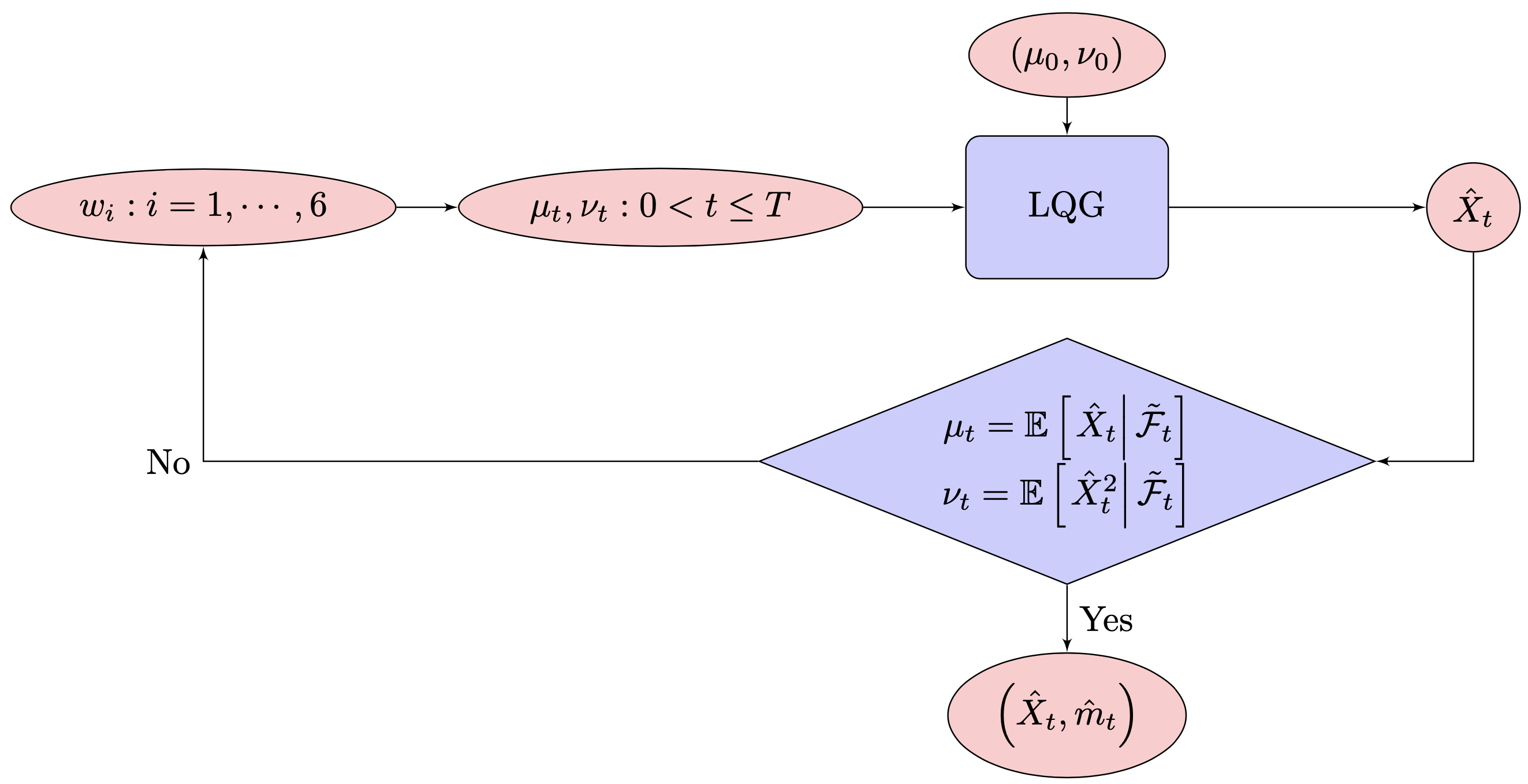
The first observation is that the cost function FF in (8) is only dependent on the measure mm through the first two moments with the quadratic cost structure, which is given by

F(x,m)=k(x22x[m]1+[m]2).F(x,m)=k(x^{2}-2x[m]_{1}+[m]_{2}).

Consequently, the underlying stochastic control problem for MFG can be entirely determined by the input given by the 2\mathbb{R}^{2} valued random processes μt=[mt]1\mu_{t}=[m_{t}]_{1} and νt=[mt]2\nu_{t}=[m_{t}]_{2}, which implies that the fixed point condition can be effectively reduced to merely checking two conditions:

μt=𝔼[X^t|~t],νt=𝔼[X^t2|~t].\mu_{t}=\mathbb{E}\left[\left.\hat{X}_{t}\right\rvert\tilde{\mathcal{F}}_{t}\right],\ \nu_{t}=\mathbb{E}\left[\left.\hat{X}_{t}^{2}\right\rvert\tilde{\mathcal{F}}_{t}\right].

This observation effectively reduces our search from the space of random measure-valued processes m:(0,T]×Ω𝒫2()m:(0,T]\times\Omega\mapsto\mathcal{P}_{2}(\mathbb{R}) to the space of 2\mathbb{R}^{2}-valued random processes (μ,ν):(0,T]×Ω2(\mu,\nu):(0,T]\times\Omega\mapsto\mathbb{R}^{2}.

It is important to note that if the underlying MFG does not involve common noise, the aforementioned observation is adequate to transform the original infinite-dimensional MFG into a finite-dimensional system. In this case, the moment processes (μ,ν)(\mu,\nu) become deterministic mappings [0,T]2[0,T]\to\mathbb{R}^{2}. However, the following example demonstrates that this is not applicable to MFG with common noise, which presents a significant drawback in characterizing LQG-MFG using a finite-dimensional system.

Example 2.

To illustrate this point, let’s consider the following uncontrolled mean field dynamics: Let the mean field term μt:=𝔼[X^t|~t]\mu_{t}:=\mathbb{E}[\hat{X}_{t}|\tilde{\mathcal{F}}_{t}], where the underlying dynamic is given by

dX^t=μtW~tdt+dWt+dW~t,X^0=X0.d\hat{X}_{t}=-\mu_{t}\tilde{W}_{t}dt+dW_{t}+d\tilde{W}_{t},\quad\hat{X}_{0}=X_{0}.

Here are two key observations:

  • μt\mu_{t} is path dependent on entire path of W~\tilde{W}, i.e.,

    μt=μ0e0tW~s𝑑s+e0tW~s𝑑s0te0sW~r𝑑r𝑑W~s.\mu_{t}=\mu_{0}e^{-\int_{0}^{t}\tilde{W}_{s}ds}+e^{-\int_{0}^{t}\tilde{W}_{s}ds}\int_{0}^{t}e^{\int_{0}^{s}\tilde{W}_{r}dr}d\tilde{W}_{s}.

    This implies that the (t,W~)μt(t,\tilde{W})\mapsto\mu_{t} is a function on an infinite dimensional domain.

  • μt\mu_{t} is Markovian, i.e.,

    dμt=μtW~tdt+dW~t.d\mu_{t}=-\mu_{t}\tilde{W}_{t}dt+d\tilde{W}_{t}.

    It is possible to express the μt\mu_{t} via a SDE with finite-dimensional coefficient functions of (t,μt)(t,\mu_{t}).

To make the previous idea more concrete, we propose the assumption of a Markovian structure for the first and second moments of the MFG equilibrium. In other words, we restrict our search for equilibrium to a smaller space \mathcal{M} of measure flows that capture the Markovian structure of the first and second moments.

Definition 4.

The space \mathcal{M} is the collection of all ~t\tilde{\mathcal{F}}_{t}-adapted measure flows m:[0,T]×Ω𝒫2()m:[0,T]\times\Omega\mapsto\mathcal{P}_{2}(\mathbb{R}), whose first moment [mt]1:=μt[m_{t}]_{1}:=\mu_{t} and second moment [mt]2:=νt[m_{t}]_{2}:=\nu_{t} satisfy a system of SDE

μt=μ0+0t(w1(s)μs+w2(s))𝑑s+W~t,\displaystyle\mu_{t}=\mu_{0}+\int_{0}^{t}\left(w_{1}(s)\mu_{s}+w_{2}(s)\right)ds+\tilde{W}_{t}, (28)
νt=ν0+0t(w3(s)μs+w4(s)νs+w5(s)μs2+w6(s))𝑑s+20tμs𝑑W~s,\displaystyle\nu_{t}=\nu_{0}+\int_{0}^{t}\left(w_{3}(s)\mu_{s}+w_{4}(s)\nu_{s}+w_{5}(s)\mu_{s}^{2}+w_{6}(s)\right)ds+2\int_{0}^{t}\mu_{s}d\tilde{W}_{s},

for some smooth deterministic functions (wi:i=1,2,,6)(w_{i}:i=1,2,\ldots,6) for all t[0,T]t\in[0,T].

Refer to caption
Figure 2: Equivalent MFG diagram with μ0=[m0]1\mu_{0}=[m_{0}]_{1} and ν0=[m0]2\nu_{0}=[m_{0}]_{2}.

The MFG problem originally given by Definition 1 can be recast as the following combination of stochastic control problem and fixed point condition:

  • RLQG(Revised LQG):

    Given smooth functions w=(wi:i=1,2,,6)w=(w_{i}:i=1,2,\ldots,6), we want to find the value function V¯=V¯[w]:[0,T]×3\bar{V}=\bar{V}[w]:[0,T]\times\mathbb{R}^{3}\to\mathbb{R} and optimal path (X^,μ^,ν^)[w](\hat{X},\hat{\mu},\hat{\nu})[w] from the following control problem:

    V¯(t,x,μ¯,ν¯)=infα𝒜𝔼[tT(12αs2+F¯(Xs,μs,νs))ds|Xt=x,μt=μ¯,νt=ν¯]\bar{V}(t,x,\bar{\mu},\bar{\nu})=\inf_{\alpha\in\mathcal{A}}\mathbb{E}\left[\left.\int_{t}^{T}\left(\frac{1}{2}\alpha_{s}^{2}+\bar{F}(X_{s},\mu_{s},\nu_{s})\right)\ ds\right\rvert X_{t}=x,\mu_{t}=\bar{\mu},\nu_{t}=\bar{\nu}\right]

    with the underlying process XX of (1) and (μ,ν)(\mu,\nu) of (28) and with the cost functions: F¯:3\bar{F}:\mathbb{R}^{3}\mapsto\mathbb{R} given by

    F¯(x,μ¯,ν¯)=k(x22xμ¯+ν¯),\bar{F}(x,\bar{\mu},\bar{\nu})=k(x^{2}-2x\bar{\mu}+\bar{\nu}),

    where μ¯,ν¯\bar{\mu},\bar{\nu} are scalars, while μ,ν\mu,\nu are used as processes.

  • RFP(Revised fixed point condition):

    Determine ww satisfying the following fixed point condition:

    μ^s=𝔼[X^s|~s] and ν^s=𝔼[X^s2|~s],s[0,T].\hat{\mu}_{s}=\mathbb{E}\left[\left.\hat{X}_{s}\right|\tilde{\mathcal{F}}_{s}\right]\hbox{ and }\hat{\nu}_{s}=\mathbb{E}\left[\left.\hat{X}_{s}^{2}\right|\tilde{\mathcal{F}}_{s}\right],\quad\forall s\in[0,T]. (29)

    The equilibrium measure is then 𝒩(μ^t,ν^tμ^t2)\mathcal{N}(\hat{\mu}_{t},\hat{\nu}_{t}-\hat{\mu}_{t}^{2}).

Remark 1.

It is important to highlight that the Markovian structure for the first and second moments of the MFG equilibrium in this manuscript differs significantly from that presented in [18]. In [18], the processes μt\mu_{t} and νt\nu_{t} are pairs of processes with finite variation, while in our case, they are quadratic variation processes.

Specifically, in [18], the coefficient functions depend on the common noise YY, whereas in (28), the coefficient functions (wi:i=1,2,,6)(w_{i}:i=1,2,\dots,6) are independent of the common noise W~\tilde{W}. Instead, the first and second moments of the MFG equilibrium are only influenced by the common noise through an additive term.

4.2 The generic player’s control with a given population measure

This section is devoted to the control problem RLQG parameterized by ww.

4.2.1 HJB equation

To simplify the notation, let’s denote each function wi(t)w_{i}(t) as wiw_{i} for i{1,2,,6}i\in\{1,2,\ldots,6\}. Assuming sufficient regularity conditions, and according to the dynamic programming principle (refer to [20] for more details), the value function V¯\bar{V} defined in the RLQG problem can be obtained as a solution vv of the following Hamilton-Jacobi-Bellman (HJB) equation

{tv+infa(axv+12a2)+(w1μ¯+w2)μ¯v+(w3μ¯+w4ν¯+w5μ¯2+w6)ν¯v+xxv+12μ¯μ¯v+xμ¯v+2μ¯2ν¯ν¯v+2μ¯μ¯ν¯v+2μ¯xν¯v+k(x22μ¯x+ν¯)=0,v(T,x,μT,νT)=0.\displaystyle\begin{cases}\vspace{4pt}\displaystyle\partial_{t}v+\inf_{a\in\mathbb{R}}\left(a\partial_{x}v+\frac{1}{2}a^{2}\right)+\left(w_{1}\bar{\mu}+w_{2}\right)\partial_{\bar{\mu}}v+\left(w_{3}\bar{\mu}+w_{4}\bar{\nu}+w_{5}\bar{\mu}^{2}+w_{6}\right)\partial_{\bar{\nu}}v+\partial_{xx}v+\frac{1}{2}\partial_{\bar{\mu}\bar{\mu}}v\\ \vspace{4pt}\displaystyle\hskip 72.26999pt+\partial_{x\bar{\mu}}v+2\bar{\mu}^{2}\partial_{\bar{\nu}\bar{\nu}}v+2\bar{\mu}\partial_{\bar{\mu}\bar{\nu}}v+2\bar{\mu}\partial_{x\bar{\nu}}v+k(x^{2}-2\bar{\mu}x+\bar{\nu})=0,\\ \displaystyle v(T,x,\mu_{T},\nu_{T})=0.\end{cases}

Therefore, the optimal control has to admit the feedback form of

α^(t)=xv(t,Xt^,μt,νt),\hat{\alpha}(t)=-\partial_{x}v\left(t,\hat{X_{t}},\mu_{t},\nu_{t}\right), (30)

and then the HJB equation can be reduced to

{tv12(xv)2+(w1μ¯+w2)μ¯v+(w3μ¯+w4ν¯+w5μ¯2+w6)ν¯v+xxv+12μ¯μ¯v+xμ¯v+2μ¯2ν¯ν¯v+2μ¯μ¯ν¯v+2μ¯xν¯v+k(x22μ¯x+ν¯)=0,v(T,x,μT,νT)=0.\displaystyle\begin{cases}\vspace{4pt}\displaystyle\partial_{t}v-\frac{1}{2}(\partial_{x}v)^{2}+\left(w_{1}\bar{\mu}+w_{2}\right)\partial_{\bar{\mu}}v+\left(w_{3}\bar{\mu}+w_{4}\bar{\nu}+w_{5}\bar{\mu}^{2}+w_{6}\right)\partial_{\bar{\nu}}v+\partial_{xx}v+\frac{1}{2}\partial_{\bar{\mu}\bar{\mu}}v\\ \vspace{4pt}\displaystyle\hskip 72.26999pt+\partial_{x\bar{\mu}}v+2\bar{\mu}^{2}\partial_{\bar{\nu}\bar{\nu}}v+2\bar{\mu}\partial_{\bar{\mu}\bar{\nu}}v+2\bar{\mu}\partial_{x\bar{\nu}}v+k(x^{2}-2\bar{\mu}x+\bar{\nu})=0,\\ \displaystyle v(T,x,\mu_{T},\nu_{T})=0.\end{cases} (31)

Next, we identify what conditions are needed for equating the control problem RLQG and the above HJB equation. Denote 𝒮\mathcal{S} to be the set of vv such that vCv\in C^{\infty} satisfies

(1+|x|2)1(|v|+|tv|)+(1+|x|+|μ|)1(|xv|+|μv|)+(|xxv|+|xμv|+|μμv|+|νv|)<K\left(1+|x|^{2}\right)^{-1}\left(|v|+|\partial_{t}v|\right)+\left(1+|x|+|\mu|\right)^{-1}\left(|\partial_{x}v|+|\partial_{\mu}v|\right)+\left(|\partial_{xx}v|+|\partial_{x\mu}v|+|\partial_{\mu\mu}v|+|\partial_{\nu}v|\right)<K

for all (t,x,μ,ν)(t,x,\mu,\nu) for some positive constant KK.

Lemma 7.

Consider the control problem RLQG with some given smooth functions w=(wi:i=1,2,,6)w=(w_{i}:i=1,2,\dots,6).

  1. 1.

    (Verification theorem) Suppose there exists a solution v𝒮v\in{\mathcal{S}} of (31). Then v(t,x,μ¯,ν¯)=V¯(t,x,μ¯,ν¯)v(t,x,\bar{\mu},\bar{\nu})=\bar{V}(t,x,\bar{\mu},\bar{\nu}), and an optimal control is provided by (30).

  2. 2.

    Suppose that the value function V¯\bar{V} belongs to 𝒮{\mathcal{S}}, and then V¯(t,x,μ¯,ν¯)\bar{V}(t,x,\bar{\mu},\bar{\nu}) solves HJB equation (31). Moreover, α^\hat{\alpha} of (30) is an optimal control.

Proof.
  1. 1.

    First, we prove the verification theorem. Since v𝒮v\in{\mathcal{S}}, for any admissible α𝔽4\alpha\in\mathcal{H}_{\mathbb{F}}^{4}, the process XαX^{\alpha} is well defined and one can apply Itô’s formula to obtain

    𝔼[v(T,XT,μT,νT)]=v(t,x,μ¯,ν¯)+𝔼[tT𝒢α(s)v(s,Xs,μs,νs)𝑑s],\mathbb{E}\left[v(T,X_{T},\mu_{T},\nu_{T})\right]=v(t,x,\bar{\mu},\bar{\nu})+\mathbb{E}\left[\int_{t}^{T}\mathcal{G}^{\alpha(s)}v(s,X_{s},\mu_{s},\nu_{s})ds\right],

    where

    𝒢af(s,x,μ¯,ν¯)\displaystyle\mathcal{G}^{a}f(s,x,\bar{\mu},\bar{\nu}) =(t+ax+xx+(w1μ¯+w2)μ¯+(w3μ¯+w4ν¯+w5μ¯2+w6)ν¯\displaystyle=\Big{(}\partial_{t}+a\partial_{x}+\partial_{xx}+\left(w_{1}\bar{\mu}+w_{2}\right)\partial_{\bar{\mu}}+\left(w_{3}\bar{\mu}+w_{4}\bar{\nu}+w_{5}\bar{\mu}^{2}+w_{6}\right)\partial_{\bar{\nu}}
    +12μ¯μ¯+2μ¯2ν¯ν¯+xμ¯+2μ¯μ¯ν¯+2μ¯xν¯)f(s,x,μ¯,ν¯).\displaystyle\hskip 36.135pt+\frac{1}{2}\partial_{\bar{\mu}\bar{\mu}}+2\bar{\mu}^{2}\partial_{\bar{\nu}\bar{\nu}}+\partial_{x\bar{\mu}}+2\bar{\mu}\partial_{\bar{\mu}\bar{\nu}}+2\bar{\mu}\partial_{x\bar{\nu}}\Big{)}f(s,x,\bar{\mu},\bar{\nu}).

    Note that the HJB equation actually implies that

    infa{𝒢av+12a2}=F¯,\inf_{a}\left\{\mathcal{G}^{a}v+\frac{1}{2}a^{2}\right\}=-\bar{F},

    which again yields

    𝒢av12a2+F¯.-\mathcal{G}^{a}v\leq\frac{1}{2}a^{2}+\bar{F}.

    Hence, we obtain that for all α𝔽4\alpha\in\mathcal{H}_{\mathbb{F}}^{4},

    v(t,x,μ¯,ν¯)\displaystyle v(t,x,\bar{\mu},\bar{\nu})
    =\displaystyle= 𝔼[tT𝒢α(s)v(s,Xs,μs,νs)ds]+𝔼[v(T,XT,μT,νT)]\displaystyle\mathbb{E}\left[\int_{t}^{T}-\mathcal{G}^{\alpha(s)}v(s,X_{s},\mu_{s},\nu_{s})ds\right]+\mathbb{E}\left[v(T,X_{T},\mu_{T},\nu_{T})\right]
    \displaystyle\leq 𝔼[tT(12α2(s)+F¯(Xs,μs,νs))𝑑s]\displaystyle\mathbb{E}\left[\int_{t}^{T}\left(\frac{1}{2}\alpha^{2}(s)+\bar{F}(X_{s},\mu_{s},\nu_{s})\right)ds\right]
    =\displaystyle= J(t,x,α,μ¯,ν¯).\displaystyle J(t,x,\alpha,\bar{\mu},\bar{\nu}).

    In the above, if α\alpha is replaced by α^\hat{\alpha} given by the feedback form (30), then since xv\partial_{x}v is Lipschitz continuous in xx, there exists corresponding optimal path X^𝔽4\hat{X}\in\mathcal{H}_{\mathbb{F}}^{4}. Thus, α^\hat{\alpha} is also in 𝔽4\mathcal{H}_{\mathbb{F}}^{4}. One can repeat all the above steps by replacing XX and α\alpha by X^\hat{X} and α^\hat{\alpha}, and \leq sign by == sign to conclude that vv is indeed the optimal value.

  2. 2.

    The opposite direction of the verification theorem follows by taking θt\theta\to t for the dynamic programming principle, for all stopping time θ[t,T],\theta\in[t,T],

    V¯(t,x,μ¯,ν¯)\displaystyle\bar{V}(t,x,\bar{\mu},\bar{\nu})
    =\displaystyle= 𝔼[tθ(12αs2+F¯(Xs,μs,νs))𝑑s+V¯(θ,Xθ,μθ,νθ)|Xt=x,μt=μ¯,νt=ν¯],\displaystyle\mathbb{E}\left[\left.\int_{t}^{\theta}\left(\frac{1}{2}\alpha_{s}^{2}+\bar{F}(X_{s},\mu_{s},\nu_{s})\right)ds+\bar{V}(\theta,X_{\theta},\mu_{\theta},\nu_{\theta})\right|X_{t}=x,\mu_{t}=\bar{\mu},\nu_{t}=\bar{\nu}\right],

    which is valid under our regularity assumptions on all the partial derivatives.

4.2.2 LQG solution

It is worth noting that the costs F¯\bar{F} of RLQG are quadratic functions in (x,μ¯,ν¯)(x,\bar{\mu},\bar{\nu}), while the drift function of the process ν\nu of (28) is not linear in (x,μ¯,ν¯)(x,\bar{\mu},\bar{\nu}). Therefore, the stochastic control problem RLQG does not fit into the typical LQG control structure. Nevertheless, similarly to the LQG solution, we guess the value function to be a quadratic function in the form of

v(t,x,μ¯,ν¯)=a(t)x2+b(t)μ¯2+c(t)ν¯+d(t)+e(t)x+f(t)μ¯+g(t)xμ¯.v(t,x,\bar{\mu},\bar{\nu})=a(t)x^{2}+b(t)\bar{\mu}^{2}+c(t)\bar{\nu}+d(t)+e(t)x+f(t)\bar{\mu}+g(t)x\bar{\mu}. (32)

Under the above setup for the value function vv, for t[0,T]t\in[0,T], the optimal control is given by

α^t=xv(t,X^t,μt,νt)=2a(t)X^te(t)g(t)μt,\hat{\alpha}_{t}=-\partial_{x}v(t,\hat{X}_{t},\mu_{t},\nu_{t})=-2a(t)\hat{X}_{t}-e(t)-g(t)\mu_{t}, (33)

and the optimal path X^\hat{X} is

{dX^t=(2a(t)X^te(t)g(t)μt)dt+dWt+dW~t,X^0=X0.\begin{cases}\vspace{4pt}\displaystyle d\hat{X}_{t}=\left(-2a(t)\hat{X}_{t}-e(t)-g(t)\mu_{t}\right)dt+dW_{t}+d\tilde{W}_{t},\\ \displaystyle\hat{X}_{0}=X_{0}.\end{cases} (34)

To proceed, we introduce the following Riccati system of ODEs for t[0,T]t\in[0,T],

{a2a2+k=0,b12g2+2bw1+cw5=0,c+cw4+k=0,d12e2+fw2+cw6+2a+b+g=0,e2ae+w2g=0,feg+w1f+2bw2+cw3=0,g2ag+w1g2k=0,\displaystyle\begin{cases}\vspace{4pt}\displaystyle a^{\prime}-2a^{2}+k=0,\\ \vspace{4pt}\displaystyle b^{\prime}-\frac{1}{2}g^{2}+2bw_{1}+cw_{5}=0,\\ \vspace{4pt}\displaystyle c^{\prime}+cw_{4}+k=0,\\ \vspace{4pt}\displaystyle d^{\prime}-\frac{1}{2}e^{2}+fw_{2}+cw_{6}+2a+b+g=0,\\ \vspace{4pt}\displaystyle e^{\prime}-2ae+w_{2}g=0,\\ \vspace{4pt}\displaystyle f^{\prime}-eg+w_{1}f+2bw_{2}+cw_{3}=0,\\ \displaystyle g^{\prime}-2ag+w_{1}g-2k=0,\end{cases} (35)

with terminal conditions

a(T)=b(T)=c(T)=d(T)=e(T)=f(T)=g(T)=0.a(T)=b(T)=c(T)=d(T)=e(T)=f(T)=g(T)=0. (36)
Lemma 8.

Suppose there exists a unique solution (a,b,c,d,e,f,g)(a,b,c,d,e,f,g) to the Riccati system of ODEs (35)-(36) on [0,T][0,T]. Then the value function of (RMFG) is given by

V¯(t,x,μ¯,ν¯)=v(t,x,μ¯,ν¯)\displaystyle\bar{V}(t,x,\bar{\mu},\bar{\nu})=v(t,x,\bar{\mu},\bar{\nu}) (37)
=\displaystyle= a(t)x2+b(t)μ¯2+c(t)ν¯+d(t)+e(t)x+f(t)μ¯+g(t)xμ¯\displaystyle a(t)x^{2}+b(t)\bar{\mu}^{2}+c(t)\bar{\nu}+d(t)+e(t)x+f(t)\bar{\mu}+g(t)x\bar{\mu}

for t[0,T]t\in[0,T] and the optimal control and optimal path are given by (33) and (34), respectively.

Proof.

With the form of value function vv given in (32) and the conditional first and second moment of X^t\hat{X}_{t} under the σ\sigma-algebra ~t\tilde{\mathcal{F}}_{t} given in (28), we have

tv=a(t)x2+e(t)x+b(t)μ¯2+f(t)μ¯+g(t)xμ¯+c(t)ν¯+d(t),\displaystyle\partial_{t}v=a^{\prime}(t)x^{2}+e^{\prime}(t)x+b^{\prime}(t)\bar{\mu}^{2}+f^{\prime}(t)\bar{\mu}+g^{\prime}(t)x\bar{\mu}+c^{\prime}(t)\bar{\nu}+d^{\prime}(t),
xv=2xa(t)+e(t)+g(t)μ¯,\displaystyle\partial_{x}v=2xa(t)+e(t)+g(t)\bar{\mu},
xxv=2a(t),\displaystyle\partial_{xx}v=2a(t),
μ¯v=2b(t)μ¯+f(t)+g(t)x,\displaystyle\partial_{\bar{\mu}}v=2b(t)\bar{\mu}+f(t)+g(t)x,
ν¯v=c(t),\displaystyle\partial_{\bar{\nu}}v=c(t),
μ¯μ¯v=2b(t),\displaystyle\partial_{\bar{\mu}\bar{\mu}}v=2b(t),
xμ¯v=g(t),\displaystyle\partial_{x\bar{\mu}}v=g(t),
μ¯ν¯v=ν¯ν¯v=xν¯v=0.\displaystyle\partial_{\bar{\mu}\bar{\nu}}v=\partial_{\bar{\nu}\bar{\nu}}v=\partial_{x\bar{\nu}}v=0.

Plugging them back to the HJB equation in (31), we get a system of ODEs in (35) by equating xx, μ¯\bar{\mu}, ν¯\bar{\nu}-like terms in each equation with the terminal conditions given in (36).

Therefore, any solution (a,b,c,d,e,f,g)(a,b,c,d,e,f,g) of a system of ODEs (35) leads to the solution of HJB (31) in the form of the quadratic function given by (37). Since the (a,b,c,d,e,f,g)(a,b,c,d,e,f,g) are differentiable functions on the closed set [0,T][0,T], they are also bounded, and thus the regularity conditions needed for v𝒮v\in\mathcal{S} is valid. Finally, we invoke the verification theorem given by Lemma 7 to conclude the desired result. ∎

4.3 Fixed point condition and the proof of Proposition 1

Returning to the ODE system (35), there are 77 equations, whereas we need to determine a total of 1313 deterministic functions of [0,T]×[0,T]\times\mathbb{R} to characterize MFG. These are

(a,b,c,d,e,f,g) and (wi:i=1,2,,6).(a,b,c,d,e,f,g)\quad\hbox{ and }\quad(w_{i}:i=1,2,\ldots,6).

In this below, we identify the missing 66 equations by checking the fixed point condition of RFP. This leads to a complete characterization of the equilibrium for MFG in Definition 1.

Lemma 9.

With the dynamic of the optimal path X^\hat{X} defined in (34), the fixed point condition (29) implies that the first moment μ^s:=𝔼[X^s|~s]\hat{\mu}_{s}:=\mathbb{E}[\hat{X}_{s}|\tilde{\mathcal{F}}_{s}] and the second moment ν^s:=𝔼[X^s2|~s]\hat{\nu}_{s}:=\mathbb{E}[\hat{X}_{s}^{2}|\tilde{\mathcal{F}}_{s}] of the optimal path conditioned on ~t\tilde{\mathcal{F}}_{t} satisfy

{μ^s=μ¯+ts((2a(r)g(r))μ^re(r))𝑑r+W~s,ν^s=ν¯+ts(24a(r)ν^r2e(r)μ^r2g(r)μ^r2)𝑑r+ts2μ^r𝑑W~r,\displaystyle\begin{cases}\vspace{4pt}\displaystyle\hat{\mu}_{s}=\bar{\mu}+\int_{t}^{s}\left(\left(-2a(r)-g(r)\right)\hat{\mu}_{r}-e(r)\right)dr+\tilde{W}_{s},\\ \displaystyle\hat{\nu}_{s}=\bar{\nu}+\int_{t}^{s}\left(2-4a(r)\hat{\nu}_{r}-2e(r)\hat{\mu}_{r}-2g(r)\hat{\mu}_{r}^{2}\right)dr+\int_{t}^{s}2\hat{\mu}_{r}d\tilde{W}_{r},\end{cases} (38)

for sts\geq t, and thus the coefficient functions w=(wi:i=1,2,,6)w=(w_{i}:i=1,2,\dots,6) in (28) satisfy the following equations:

w1=2ag,w2=e,w3=2e,w4=4a,w5=2g,w6=2,t[0,T].w_{1}=-2a-g,\ w_{2}=-e,\ w_{3}=-2e,\ w_{4}=-4a,\ w_{5}=-2g,\ w_{6}=2,\quad\forall t\in[0,T]. (39)
Proof.

With the dynamic of the optimal path X^\hat{X} given by (34), we have

X^t=X0+0t(2a(s)X^se(s)g(s)μ^s)𝑑s+Wt+W~t,\hat{X}_{t}=X_{0}+\int_{0}^{t}\left(-2a(s)\hat{X}_{s}-e(s)-g(s)\hat{\mu}_{s}\right)ds+W_{t}+\tilde{W}_{t},

and since the functions a,e,ga,e,g are continuous on [0,T][0,T], then we can change of order of integration and expectation and it yields

μ^t\displaystyle\hat{\mu}_{t} =𝔼[X^t|~t]\displaystyle=\mathbb{E}\left[\left.\hat{X}_{t}\right|\tilde{\mathcal{F}}_{t}\right]
=𝔼[X0|~t]+0t(2a(s)μ^se(s)g(s)μ^s)𝑑s+𝔼[Wt|~t]+𝔼[W~t|~t]\displaystyle=\mathbb{E}\left[\left.X_{0}\right|\tilde{\mathcal{F}}_{t}\right]+\int_{0}^{t}\left(-2a(s)\hat{\mu}_{s}-e(s)-g(s)\hat{\mu}_{s}\right)ds+\mathbb{E}\left[\left.W_{t}\right|\tilde{\mathcal{F}}_{t}\right]+\mathbb{E}\left[\left.\tilde{W}_{t}\right|\tilde{\mathcal{F}}_{t}\right]
=𝔼[X0|~t]+0t(2a(s)μ^se(s)g(s)μ^s)𝑑s+W~t.\displaystyle=\mathbb{E}\left[\left.X_{0}\right|\tilde{\mathcal{F}}_{t}\right]+\int_{0}^{t}\left(-2a(s)\hat{\mu}_{s}-e(s)-g(s)\hat{\mu}_{s}\right)ds+\tilde{W}_{t}.

Similarly, applying Itô’s formula, we obtain

X^t2=X02+0t(24a(s)X^s22e(s)X^s2g(s)μ^sX^s)𝑑s+0t2X^s𝑑Ws+0t2X^s𝑑W~s,\hat{X}_{t}^{2}=X_{0}^{2}+\int_{0}^{t}\left(2-4a(s)\hat{X}_{s}^{2}-2e(s)\hat{X}_{s}-2g(s)\hat{\mu}_{s}\hat{X}_{s}\right)ds+\int_{0}^{t}2\hat{X}_{s}dW_{s}+\int_{0}^{t}2\hat{X}_{s}d\tilde{W}_{s},

and it follows that

ν^t\displaystyle\hat{\nu}_{t} =𝔼[X^t2|~t]\displaystyle=\mathbb{E}\left[\left.\hat{X}_{t}^{2}\right|\tilde{\mathcal{F}}_{t}\right]
=𝔼[X02|~t]+0t(24a(s)ν^s2e(s)μ^s2g(s)μ^s2)𝑑s+𝔼[0t2X^s𝑑Ws|~t]+𝔼[0t2X^s𝑑W~s|~t]\displaystyle=\mathbb{E}\left[\left.X_{0}^{2}\right|\tilde{\mathcal{F}}_{t}\right]+\int_{0}^{t}\left(2-4a(s)\hat{\nu}_{s}-2e(s)\hat{\mu}_{s}-2g(s)\hat{\mu}_{s}^{2}\right)ds+\mathbb{E}\left[\left.\int_{0}^{t}2\hat{X}_{s}dW_{s}\right|\tilde{\mathcal{F}}_{t}\right]+\mathbb{E}\left[\left.\int_{0}^{t}2\hat{X}_{s}d\tilde{W}_{s}\right|\tilde{\mathcal{F}}_{t}\right]
=𝔼[X02|~t]+0t(24a(s)ν^s2e(s)μ^s2g(s)μ^s2)𝑑s+0t2μ^s𝑑W~s.\displaystyle=\mathbb{E}\left[\left.X_{0}^{2}\right|\tilde{\mathcal{F}}_{t}\right]+\int_{0}^{t}\left(2-4a(s)\hat{\nu}_{s}-2e(s)\hat{\mu}_{s}-2g(s)\hat{\mu}_{s}^{2}\right)ds+\int_{0}^{t}2\hat{\mu}_{s}d\tilde{W}_{s}.

Thus the desired result in (38) is obtained. Next, comparing the terms in (28) and (38), to satisfy the fixed point condition in MFG, we require another 66 equations in (39) for the coefficient functions w=(wi:i=1,2,,6)w=(w_{i}:i=1,2,\dots,6). ∎

Using further algebraic structures, one can reduce the ODE system of 1313 equations composed by (35) and (39) into a system of 44 equations.

Proof of Proposition 1.

Let the smooth and bounded functions {wi:i=1,2,,6}\{w_{i}:i=1,2,\dots,6\} be given, the functions (a,b,c,d,e,f,g)\left(a,b,c,d,e,f,g\right) in (35) is a coupled linear system, and thus their existence, uniqueness and boundedness is shown by Theorem 12.1 in [1].

Plugging the 66 equations in (39) to the ODE system (35), we obtain

{a2a2+k=0,b12g24ab2bg2cg=0,c4ac+k=0,d12e2ef+2c+2a+b+g=0,e2aeeg=0,feg2afgf2be2ce=0,g4agg22k=0,\displaystyle\begin{cases}\vspace{4pt}\displaystyle a^{\prime}-2a^{2}+k=0,\\ \vspace{4pt}\displaystyle b^{\prime}-\frac{1}{2}g^{2}-4ab-2bg-2cg=0,\\ \vspace{4pt}\displaystyle c^{\prime}-4ac+k=0,\\ \vspace{4pt}\displaystyle d^{\prime}-\frac{1}{2}e^{2}-ef+2c+2a+b+g=0,\\ \vspace{4pt}\displaystyle e^{\prime}-2ae-eg=0,\\ \vspace{4pt}\displaystyle f^{\prime}-eg-2af-gf-2be-2ce=0,\\ \vspace{4pt}\displaystyle g^{\prime}-4ag-g^{2}-2k=0,\end{cases}

with the terminal conditions

a(T)=b(T)=c(T)=d(T)=e(T)=f(T)=g(T)=0.a(T)=b(T)=c(T)=d(T)=e(T)=f(T)=g(T)=0.

Let l=2a+gl=2a+g, and it easily to obtain

l(t)l2(t)=0,l(T)=0,l^{\prime}(t)-l^{2}(t)=0,\quad l(T)=0,

which implies that l(t)=2a(t)+g(t)=0l(t)=2a(t)+g(t)=0 for all t[0,T]t\in[0,T]. This gives the result that g=2ag=-2a and it yields e=0e^{\prime}=0. Then with e(T)=0e(T)=0, we have e(t)=0e(t)=0 for all t[0,T]t\in[0,T] and thus one can obtain f=0f^{\prime}=0, which indicates that f(t)=0f(t)=0 for all t[0,T]t\in[0,T] as f(T)=0f(T)=0. Therefore the ODE system (35) can be simplified to the following form about (a(t),b(t),c(t),d(t):t[0,T])\left(a(t),b(t),c(t),d(t):t\in[0,T]\right):

{a(t)2a2(t)+k=0,b(t)2a2(t)+4a(t)c(t)=0,c(t)4a(t)c(t)+k=0,d(t)+b(t)+2c(t)=0,\displaystyle\begin{cases}\vspace{4pt}\displaystyle a^{\prime}(t)-2a^{2}(t)+k=0,\\ \vspace{4pt}\displaystyle b^{\prime}(t)-2a^{2}(t)+4a(t)c(t)=0,\\ \vspace{4pt}\displaystyle c^{\prime}(t)-4a(t)c(t)+k=0,\\ \displaystyle d^{\prime}(t)+b(t)+2c(t)=0,\end{cases} (40)

with the terminal conditions

a(T)=b(T)=c(T)=d(T)=0.a(T)=b(T)=c(T)=d(T)=0. (41)

The unique solvability of the Riccati system (40)-(41) is proven in Lemma 12 in the Appendix. Note that the solution aa of (11) is consistent with the solution of the Riccati system given by equations (40)-(41).

In this case, since 2a+g=02a+g=0 and e=0e=0 for all t[0,T]t\in[0,T], it follows that μ^s=μ¯+W~s\hat{\mu}_{s}=\bar{\mu}+\tilde{W}_{s} for all s[t,T]s\in[t,T] from the fixed point result (38). Similarly,

ν^s=ν¯+ts(2+4a(r)μ^r24a(r)ν^r)𝑑r+ts2μ^r𝑑W~r,s[t,T].\hat{\nu}_{s}=\bar{\nu}+\int_{t}^{s}\left(2+4a(r)\hat{\mu}_{r}^{2}-4a(r)\hat{\nu}_{r}\right)\,dr+\int_{t}^{s}2\hat{\mu}_{r}\,d\tilde{W}_{r},\quad\forall s\in[t,T].

Plugging e=0e=0 and μ^s=μ¯+W~r\hat{\mu}_{s}=\bar{\mu}+\tilde{W}_{r} back to (33), we obtain the optimal control by

α^s=2a(s)(μ¯+W~sX^s).\hat{\alpha}_{s}=2a(s)(\bar{\mu}+\tilde{W}_{s}-\hat{X}_{s}).

Moreover, since e=f=0e=f=0 and g=2ag=-2a for s[t,T]s\in[t,T], the value function can be simplified from (32) to

v(t,x,μ¯,ν¯)=a(t)x22a(t)xμ¯+b(t)μ¯2+c(t)ν¯+d(t).v(t,x,\bar{\mu},\bar{\nu})=a(t)x^{2}-2a(t)x\bar{\mu}+b(t)\bar{\mu}^{2}+c(t)\bar{\nu}+d(t).

This concludes Proposition 1.

5 The NN-Player Game

This section focuses on proving Proposition 2 regarding the corresponding NN-player game. For simplicity, we can omit the superscript (N)(N) when referring to the processes in the sample space Ω(N)\Omega^{(N)}.

To begin, we address the NN-player game in Subsection 5.1, where we solve it and obtain a Riccati system containing O(N3)O(N^{3}) equations. Subsequently, we reduce the relevant Riccati system to an ODE system in Subsection 5.2, which has a dimension independent of NN. This simplified system forms the fundamental component of the convergence result.

5.1 Characterization of the NN-player game by Riccati system

It is important to emphasize that based on the problem setting in Subsection 2.2 and the running cost for each player specified in (9), the NN-player game can be classified as an NN-coupled stochastic LQG problem. As a result, the value function and optimal control for each player can be determined by means of the following Riccati system:

For i=1,2,,Ni=1,2,\ldots,N, consider

{Ai2AieieiAi4jiNAjejejAi+kNjiN(eiej)(eiej)=0,Bi2AieieiBi2jiN(AiejejBj+AjejejBi)=0,Ci12BieieiBijiNBjejejBi+2tr(Ai)=0,Ai(T)=Bi(T)=Ci(T)=0,\begin{cases}\vspace{4pt}\displaystyle A_{i}^{\prime}-2A_{i}^{\top}e_{i}e_{i}^{\top}A_{i}-4\sum_{j\neq i}^{N}A_{j}^{\top}e_{j}e_{j}^{\top}A_{i}+\frac{k}{N}\sum_{j\neq i}^{N}\left(e_{i}-e_{j}\right)\left(e_{i}-e_{j}\right)^{\top}=0,\\ \vspace{4pt}\displaystyle B_{i}^{\prime}-2A_{i}^{\top}e_{i}e_{i}^{\top}B_{i}-2\sum_{j\neq i}^{N}\left(A_{i}^{\top}e_{j}e_{j}^{\top}B_{j}+A_{j}^{\top}e_{j}e_{j}^{\top}B_{i}\right)=0,\\ \vspace{4pt}\displaystyle C_{i}^{\prime}-\frac{1}{2}B_{i}^{\top}e_{i}e_{i}^{\top}B_{i}-\sum_{j\neq i}^{N}B_{j}^{\top}e_{j}e_{j}^{\top}B_{i}+2tr(A_{i})=0,\\ \displaystyle A_{i}(T)=B_{i}(T)=C_{i}(T)=0,\end{cases} (42)

where AiA_{i} is N×NN\times N symmetric matrix, BiB_{i} is NN-dimensional vector, CiC_{i}\in\mathbb{R} is a real constant, and eie_{i} is the ii-th natural basis in N\mathbb{R}^{N} for each i=1,2,,Ni=1,2,\dots,N.

Lemma 10.

Suppose (Ai,Bi,Ci:i=1,2,,N)(A_{i},B_{i},C_{i}:i=1,2,\ldots,N) is the solution of the Riccati system (42). Then, the value functions of NN-player game defined by (7) is

Vi(x(N))=(x(N))Ai(0)x(N)+(x(N))Bi(0)+Ci(0),i=1,2,,N.V_{i}\left(x^{(N)}\right)=\left(x^{(N)}\right)^{\top}A_{i}(0)x^{(N)}+\left(x^{(N)}\right)^{\top}B_{i}(0)+C_{i}(0),\quad i=1,2,\ldots,N.

Moreover, the path and the control under the equilibrium are given by

dX^it(N)=(2(Ai(t))iX^t(N)(Bi(t))i)dt+dWit(N)+dW~t,d\hat{X}_{it}^{(N)}=\left(-2(A_{i}(t))_{i}^{\top}\hat{X}_{t}^{(N)}-(B_{i}(t))_{i}\right)dt+dW^{(N)}_{it}+d\tilde{W}_{t}, (43)

and

α^it(N)=2(Ai(t))iX^t(N)(Bi(t))i\hat{\alpha}^{(N)}_{it}=-2(A_{i}(t))_{i}^{\top}\hat{X}^{(N)}_{t}-(B_{i}(t))_{i}

for each i=1,2,,Ni=1,2,\dots,N, where (A)i(A)_{i} denotes the ii-th column of matrix AA, (B)i(B)_{i} denotes the ii-th entry of vector BB and X^t(N)=[X^1t(N),X^2t(N),,X^Nt(N)]\hat{X}^{(N)}_{t}=[\hat{X}^{(N)}_{1t},\hat{X}^{(N)}_{2t},\dots,\hat{X}^{(N)}_{Nt}]^{\top}.

Proof.

From the dynamic programming principle, it is standard that, under enough regularities, the players’ value function V(x(N))=(V1,V2,,VN)(x(N))V(x^{(N)})=(V_{1},V_{2},\dots,V_{N})(x^{(N)}) can be lifted to the solution vi(t,x(N))v_{i}(t,x^{(N)}) of the following system of HJB equations, for i=1,2,,Ni=1,2,\dots,N,

{tvi+infait(aitxivi+12ait2)+jiNajtxjvi+Δvi+kNjiN((eiej)x(N))2=0,vi(T,x(N))=0.\displaystyle\begin{cases}\vspace{4pt}\displaystyle\partial_{t}v_{i}+\inf_{a_{it}\in\mathbb{R}}\left(a_{it}\partial_{x_{i}}v_{i}+\frac{1}{2}a_{it}^{2}\right)+\sum_{j\neq i}^{N}a_{jt}\partial_{x_{j}}v_{i}+\Delta v_{i}+\frac{k}{N}\sum_{j\neq i}^{N}\left(\left(e_{i}-e_{j}\right)^{\top}x^{(N)}\right)^{2}=0,\\ \displaystyle v_{i}\left(T,x^{(N)}\right)=0.\end{cases}

Note that with ait=xivi(t,x(N))a_{it}=-\partial_{x_{i}}v_{i}\left(t,x^{(N)}\right) for each i=1,2,,Ni=1,2,\dots,N, the term in the infimum attains the optimal value and thus the HJB equation can be reduced to

{tvi12(xivi)2jiNxjvjxjvi+Δvi+kNjiN((eiej)x(N))2=0,vi(T,x(N))=0.\displaystyle\begin{cases}\vspace{4pt}\displaystyle\partial_{t}v_{i}-\frac{1}{2}\left(\partial_{x_{i}}v_{i}\right)^{2}-\sum_{j\neq i}^{N}\partial_{x_{j}}v_{j}\partial_{x_{j}}v_{i}+\Delta v_{i}+\frac{k}{N}\sum_{j\neq i}^{N}\left(\left(e_{i}-e_{j}\right)^{\top}x^{(N)}\right)^{2}=0,\\ \displaystyle v_{i}\left(T,x^{(N)}\right)=0.\end{cases} (44)

Then, the value functions VV of NN-player game defined by (7) is Vi(x(N))=vi(0,x(N))V_{i}(x^{(N)})=v_{i}(0,x^{(N)}) for all i=1,2,,Ni=1,2,\dots,N. Moreover, the path and the control under the equilibrium are given by

dX^it(N)=xivi(t,X^t(N))dt+dWit(N)+dW~t,d\hat{X}^{(N)}_{it}=-\partial_{x_{i}}v_{i}\left(t,\hat{X}^{(N)}_{t}\right)dt+dW^{(N)}_{it}+d\tilde{W}_{t},

and

α^it(N)=xivi(t,X^t(N))\hat{\alpha}^{(N)}_{it}=-\partial_{x_{i}}v_{i}\left(t,\hat{X}^{(N)}_{t}\right)

for i=1,2,,Ni=1,2,\dots,N. The proof is the application of Itô’s formula and the details are omitted here. Due to its LQG structure, the value function leads to a quadratic function of the form

vi(t,x(N))=(x(N))Ai(t)x(N)+(x(N))Bi(t)+Ci(t).v_{i}\left(t,x^{(N)}\right)=\left(x^{(N)}\right)^{\top}A_{i}(t)x^{(N)}+\left(x^{(N)}\right)^{\top}B_{i}(t)+C_{i}(t).

Plugging ViV_{i} into (44), and matching the coefficient of variables, we get the Riccati system of ODEs in (42) and the desired results are obtained. ∎

5.2 Proof of Proposition 2: Reduced Riccati form for the equilibrium

At present, the MFG and the corresponding NN-player game can be characterized by Proposition 1 and Lemma 10, respectively. One of our primary objectives is to examine the convergence of the representative optimal path X^1t(N)\hat{X}_{1t}^{(N)} generated by the NN-player game defined in (42)-(43) to the optimal path X^t\hat{X}_{t} of the MFG described in Proposition 1.

It should be noted that X^t\hat{X}_{t} is solely dependent on the function a(t)a(t), as indicated in the ODE (11). In contrast, X^1t(N)\hat{X}_{1t}^{(N)} depends on O(N3)O(N^{3}) many functions derived from the solutions of a substantial Riccati system (42) involving matrices (Ait,Bit:i=1,2,,N)(A_{it},B_{it}:i=1,2,\dots,N). Consequently, comparing these two processes meaningfully becomes an exceedingly challenging task without gaining further insight into the intricate structure of the Riccati system (42).

Proof of Proposition 2.

Inspired from the setup in [18] and [16], we may seek a pattern for the matrix AiA_{i} in the following form:

(Ai)pq={a1(t), if p=q=i,a2(t), if p=qi,a3(t), if pq,p=i or q=i,a4(t), otherwise.(A_{i})_{pq}=\begin{cases}a_{1}(t),&\text{ if }p=q=i,\\ a_{2}(t),&\text{ if }p=q\neq i,\\ a_{3}(t),&\text{ if }p\neq q,p=i\text{ or }q=i,\\ a_{4}(t),&\text{ otherwise}.\end{cases} (45)

The next result justifies the above pattern: the N2N^{2} entries of the matrix AiA_{i} can be embedded to a 22-dimensional vector space no matter how big NN is.

For the Riccati system (42), with the given of AiA_{i} and suppose each function in AiA_{i} is continuous on [0,T][0,T], it is obvious to see that Bi=0B_{i}=0 for all t[0,T]t\in[0,T] and for all i=1,2,,Ni=1,2,\dots,N. Note that in this case, for i=1,2,,Ni=1,2,\dots,N, the optimal control is given by

α^i=2j=1N(Ai)ijX^jt(N)=2(Ai)iX^t(N),\hat{\alpha}_{i}=-2\sum_{j=1}^{N}(A_{i})_{ij}\hat{X}_{jt}^{(N)}=-2\left(A_{i}\right)_{i}^{\top}\hat{X}^{(N)}_{t},

where (A)i(A)_{i} is the ii-th column of matrix AA.

Plugging the pattern (45) into the differential equation of AiA_{i}, we obtain the following system of ODEs:

{a12a124(N1)a32+N1Nk=0,a22a324a1a24(N2)a3a4+kN=0,a32a1a34a1a34(N2)a32kN=0,a32a1a34a2a34(N2)a3a4kN=0,a42a324a2a34a1a44(N3)a3a4=0\displaystyle\begin{cases}\vspace{4pt}\displaystyle a_{1}^{\prime}-2a_{1}^{2}-4(N-1)a_{3}^{2}+\frac{N-1}{N}k=0,\\ \vspace{4pt}\displaystyle a_{2}^{\prime}-2a_{3}^{2}-4a_{1}a_{2}-4(N-2)a_{3}a_{4}+\frac{k}{N}=0,\\ \vspace{4pt}\displaystyle a_{3}^{\prime}-2a_{1}a_{3}-4a_{1}a_{3}-4(N-2)a_{3}^{2}-\frac{k}{N}=0,\\ \vspace{4pt}\displaystyle a_{3}^{\prime}-2a_{1}a_{3}-4a_{2}a_{3}-4(N-2)a_{3}a_{4}-\frac{k}{N}=0,\\ \displaystyle a_{4}^{\prime}-2a_{3}^{2}-4a_{2}a_{3}-4a_{1}a_{4}-4(N-3)a_{3}a_{4}=0\end{cases}

with the terminal conditions

a1(T)=a2(T)=a3(T)=a4(T)=0.a_{1}(T)=a_{2}(T)=a_{3}(T)=a_{4}(T)=0.

It is worth noting that there are two ODEs for a3a_{3}, and the two expressions should be equal, thus

a1a3+(N2)a32=a2a3+(N2)a3a4,a_{1}a_{3}+(N-2)a_{3}^{2}=a_{2}a_{3}+(N-2)a_{3}a_{4},

which implies that (a1+(N2)a3)=(a2+(N2)a4)\left(a_{1}+(N-2)a_{3}\right)^{\prime}=\left(a_{2}+(N-2)a_{4}\right)^{\prime} or

2a12+2(N2)a1a3+4(N1)a32+4(N2)a2a3+4(N2)2a3a4kN\displaystyle 2a_{1}^{2}+2(N-2)a_{1}a_{3}+4(N-1)a_{3}^{2}+4(N-2)a_{2}a_{3}+4(N-2)^{2}a_{3}a_{4}-\frac{k}{N}
=\displaystyle= 2(N1)a32+4a1a2+4(N2)(a2a3+a3a4+a1a4)+4(N2)(N3)a3a4kN.\displaystyle 2(N-1)a_{3}^{2}+4a_{1}a_{2}+4(N-2)(a_{2}a_{3}+a_{3}a_{4}+a_{1}a_{4})+4(N-2)(N-3)a_{3}a_{4}-\frac{k}{N}.

After combining terms and substituting a2+(N2)a4a_{2}+(N-2)a_{4} with a1+(N2)a3a_{1}+(N-2)a_{3}, we get

a12+(N2)a1a3(N1)a32=0,a_{1}^{2}+(N-2)a_{1}a_{3}-(N-1)a_{3}^{2}=0,

which yields a3=a1a_{3}=a_{1} or a3=1N1a1a_{3}=-\frac{1}{N-1}a_{1}. Note that, since a1a_{1} and a3a_{3} satisfies different differential equations, it follows that a3a1a_{3}\neq a_{1}. Hence, we can conclude that a3=1N1a1a_{3}=-\frac{1}{N-1}a_{1}. Next, from the equation a1+(N2)a3=a2+(N2)a4a_{1}+(N-2)a_{3}=a_{2}+(N-2)a_{4}, we have

a4=1N2a1+a31N2a2.a_{4}=\frac{1}{N-2}a_{1}+a_{3}-\frac{1}{N-2}a_{2}.

In conclusion, for i=1,2,,Ni=1,2,\dots,N, AiA_{i} has the following expressions:

(Ai)pq={a1(t), if p=q=i,a2(t), if p=qi,1N1a1(t), if pq,p=i or q=i,1(N1)(N2)a1(t)1N2a2(t), otherwise,(A_{i})_{pq}=\begin{cases}\vspace{4pt}\displaystyle a_{1}(t),&\text{ if }p=q=i,\\ \vspace{4pt}\displaystyle a_{2}(t),&\text{ if }p=q\neq i,\\ \vspace{4pt}\displaystyle-\frac{1}{N-1}a_{1}(t),&\text{ if }p\neq q,p=i\text{ or }q=i,\\ \displaystyle\frac{1}{(N-1)(N-2)}a_{1}(t)-\frac{1}{N-2}a_{2}(t),&\text{ otherwise},\end{cases}

where a1a_{1} and a2a_{2} satisfies the system of ODEs (46)

{a12(N+1)N1a12+N1Nk=0,a2+2(N1)2a124NN1a1a2+kN=0,a1(T)=a2(T)=0.\begin{cases}\vspace{4pt}\displaystyle a_{1}^{\prime}-\frac{2(N+1)}{N-1}a_{1}^{2}+\frac{N-1}{N}k=0,\\ \vspace{4pt}\displaystyle a_{2}^{\prime}+\frac{2}{(N-1)^{2}}a_{1}^{2}-\frac{4N}{N-1}a_{1}a_{2}+\frac{k}{N}=0,\\ \displaystyle a_{1}(T)=a_{2}(T)=0.\end{cases} (46)

The existence and uniqueness of AiA_{i} in (42) are equivalent to the existence and uniqueness of (46). Firstly, the existence, uniqueness, and boundness of a1a_{1} in (46) is from the same argument for aa in (40), which is shown as the proof of Lemma 12 in Appendix. The explicit solution of a1a_{1} is given by

a1(t)=k2(N1)2N(N+1)1e22N+1Nk(Tt)1+e22N+1Nk(Tt)a_{1}(t)=\sqrt{\frac{k}{2}\frac{(N-1)^{2}}{N(N+1)}}\frac{1-e^{-2\sqrt{2}\sqrt{\frac{N+1}{N}k}(T-t)}}{1+e^{-2\sqrt{2}\sqrt{\frac{N+1}{N}k}(T-t)}}

for all t[0,T]t\in[0,T]. Next, with the given of a1a_{1}, the existence, uniqueness, and boundness of a2a_{2} in (46) is guaranteed by Theorem 12.1 in [1]. Therefore, we can express the equilibrium paths and associated controls as the following:

dX^it(N)=2a1N(t)(X^it(N)1N1jiNX^jt(N))dt+dWit(N)+dW~t,d\hat{X}_{it}^{(N)}=-2a_{1}^{N}(t)\left(\hat{X}_{it}^{(N)}-\frac{1}{N-1}\sum_{j\neq i}^{N}\hat{X}_{jt}^{(N)}\right)dt+dW_{it}^{(N)}+d\tilde{W}_{t}, (47)

and

α^it(N)=2a1N(t)(X^it(N)1N1jiNX^jt(N))\hat{\alpha}_{it}^{(N)}=-2a_{1}^{N}(t)\left(\hat{X}_{it}^{(N)}-\frac{1}{N-1}\sum_{j\neq i}^{N}\hat{X}_{jt}^{(N)}\right)

respectively for i=1,2,,Ni=1,2,\dots,N, where a1Na_{1}^{N} is the solution to the ODE for a1a_{1} in (46). This concludes Proposition 2. ∎

6 Further remark

We have now established Proposition 1 concerning the MFG in Section 4 and Proposition 2 regarding the NN-player game in Section 5. With these propositions proven, we are now able to conclude the proof of Theorem 1, which was presented in Section 3.4.

7 Appendix

Lemma 11.

Let 𝕎p\mathbb{W}_{p} be the pp-Wasserstein metric. If XX and YY are two real-valued random variables and cc is a constant, then

𝕎p((X),(Y))=𝕎p((X+c),(Y+c)).\mathbb{W}_{p}(\mathcal{L}(X),\mathcal{L}(Y))=\mathbb{W}_{p}(\mathcal{L}(X+c),\mathcal{L}(Y+c)). (48)

Moreover, if α={αi:i}\alpha=\{\alpha_{i}:i\in\mathbb{N}\} is a sequence of random variables, then

𝕎p(1Ni=1Nδαi+c,(Y+c))=𝕎p(1Ni=1Nδαi,(Y)).\mathbb{W}_{p}\left(\frac{1}{N}\sum_{i=1}^{N}\delta_{\alpha_{i}+c},\mathcal{L}(Y+c)\right)=\mathbb{W}_{p}\left(\frac{1}{N}\sum_{i=1}^{N}\delta_{\alpha_{i}},\mathcal{L}(Y)\right). (49)
Proof.

By definition of the pp-Wasserstein metric, we have:

𝕎p((X),(Y))=(infπΠ((X),(Y))2|xy|p𝑑π(x,y))1p,\mathbb{W}_{p}(\mathcal{L}(X),\mathcal{L}(Y))=\left(\inf_{\pi\in\Pi(\mathcal{L}(X),\mathcal{L}(Y))}\int_{\mathbb{R}^{2}}|x-y|^{p}d\pi(x,y)\right)^{\frac{1}{p}},

where Π((X),(Y))\Pi(\mathcal{L}(X),\mathcal{L}(Y)) is the set of all joint probability measures with marginals (X)\mathcal{L}(X) and (Y)\mathcal{L}(Y). Similarly,

𝕎p((X+c),(Y+c))=(infπΠ((X+c),(Y+c))2|xy|p𝑑π(x,y))1p,\mathbb{W}_{p}(\mathcal{L}(X+c),\mathcal{L}(Y+c))=\left(\inf_{\pi\in\Pi(\mathcal{L}(X+c),\mathcal{L}(Y+c))}\int_{\mathbb{R}^{2}}|x-y|^{p}d\pi(x,y)\right)^{\frac{1}{p}},

where Π((X+c),(Y+c))\Pi(\mathcal{L}(X+c),\mathcal{L}(Y+c)) is the set of all joint probability measures with marginals (X+c)\mathcal{L}(X+c) and (Y+c)\mathcal{L}(Y+c).

Now, consider the mapping Φ:22\Phi:\mathbb{R}^{2}\to\mathbb{R}^{2} given by Φ(x,y)=(x+c,y+c)\Phi(x,y)=(x+c,y+c). For any πΠ((X),(Y))\pi\in\Pi(\mathcal{L}(X),\mathcal{L}(Y)), the pushforward measure of π\pi under Φ\Phi belongs to Π((X+c),(Y+c))\Pi(\mathcal{L}(X+c),\mathcal{L}(Y+c)), i.e., π=ΦπΠ((X+c),(Y+c))\pi^{\prime}=\Phi_{*}\pi\in\Pi(\mathcal{L}(X+c),\mathcal{L}(Y+c)). Thus, we have

ΦΠ((X),(Y))Π((X+c),(Y+c)).\Phi_{*}\Pi(\mathcal{L}(X),\mathcal{L}(Y))\subset\Pi(\mathcal{L}(X+c),\mathcal{L}(Y+c)).

Moreover, Φ\Phi is bijective and measure preserving, then

2|xy|p𝑑π(x,y)=2|(x+c)(y+c)|p𝑑π(x,y)=2|xy|p𝑑π(x,y).\int_{\mathbb{R}^{2}}|x-y|^{p}d\pi^{\prime}(x,y)=\int_{\mathbb{R}^{2}}|(x+c)-(y+c)|^{p}d\pi(x,y)=\int_{\mathbb{R}^{2}}|x-y|^{p}d\pi(x,y).

Therefore, we know that

𝕎pp((X),(Y))\displaystyle\mathbb{W}_{p}^{p}\left(\mathcal{L}(X),\mathcal{L}(Y)\right) =infπΠ((X),(Y))2|xy|p𝑑π(x,y)\displaystyle=\inf_{\pi\in\Pi(\mathcal{L}(X),\mathcal{L}(Y))}\int_{\mathbb{R}^{2}}|x-y|^{p}d\pi(x,y)
=infπΠ((X),(Y))2|xy|p𝑑Φπ(x,y)\displaystyle=\inf_{\pi\in\Pi(\mathcal{L}(X),\mathcal{L}(Y))}\int_{\mathbb{R}^{2}}|x-y|^{p}d\Phi_{*}\pi(x,y)
=infπΦΠ((X),(Y))2|xy|p𝑑π(x,y)\displaystyle=\inf_{\pi^{\prime}\in\Phi_{*}\Pi(\mathcal{L}(X),\mathcal{L}(Y))}\int_{\mathbb{R}^{2}}|x-y|^{p}d\pi^{\prime}(x,y)
𝕎pp((X+c),(Y+c)).\displaystyle\geq\mathbb{W}_{p}^{p}(\mathcal{L}(X+c),\mathcal{L}(Y+c)).

by the definition of the pp-Wasserstein metric. If we apply the above inequality to X=X+cX^{\prime}=X+c, Y=Y+cY^{\prime}=Y+c, and c=cc^{\prime}=-c, the opposite inequality is provided. Thus, it completes the proof of (48).

Next, we note that

1Ni=1Nδαi+c=(αu+c|α),\frac{1}{N}\sum_{i=1}^{N}\delta_{\alpha_{i}+c}=\mathcal{L}(\alpha_{u}+c|\alpha),

where uu be a uniform random variable on {1,2,,N}\{1,2,\dots,N\} independent to α\alpha. Using (48), we conclude (49) from

𝕎p(1Ni=1Nδαi+c,(Y+c))\displaystyle\mathbb{W}_{p}\left(\frac{1}{N}\sum_{i=1}^{N}\delta_{\alpha_{i}+c},\mathcal{L}(Y+c)\right) =𝕎p((αu+c|α),(Y+c))\displaystyle=\mathbb{W}_{p}\left(\mathcal{L}(\alpha_{u}+c|\alpha),\mathcal{L}(Y+c)\right)
=𝕎p((αu|α),(Y))\displaystyle=\mathbb{W}_{p}\left(\mathcal{L}(\alpha_{u}|\alpha),\mathcal{L}(Y)\right)
=𝕎p(1Ni=1Nδαi,(Y)).\displaystyle=\mathbb{W}_{p}\left(\frac{1}{N}\sum_{i=1}^{N}\delta_{\alpha_{i}},\mathcal{L}(Y)\right).

Lemma 12.

Under the Assumption 2, there exists a unique solution (a(t),b(t),c(t),d(t):t[0,T])\left(a(t),b(t),c(t),d(t):t\in[0,T]\right) for the Riccati system of ODEs (40)-(41) and the solution can given explicitly by

{a(t)=k21e22k(Tt)1+e22k(Tt),b(t)=tT(4a(s)c(s)2a2(s))𝑑s,c(t)=ktTets4a(r)dr𝑑s,d(t)=tT(b(s)+2c(s))𝑑s.\begin{cases}\vspace{4pt}\displaystyle a(t)=\sqrt{\frac{k}{2}}\frac{1-e^{-2\sqrt{2k}(T-t)}}{1+e^{-2\sqrt{2k}(T-t)}},\\ \vspace{4pt}\displaystyle b(t)=\int_{t}^{T}\left(4a(s)c(s)-2a^{2}(s)\right)ds,\\ \vspace{4pt}\displaystyle c(t)=k\int_{t}^{T}e^{\int_{t}^{s}-4a(r)dr}ds,\\ \displaystyle d(t)=\int_{t}^{T}\left(b(s)+2c(s)\right)ds.\end{cases}
Proof.

Firstly, with the given of k>0k>0, we can solve the ODE

a(t)2a2(t)+k=0,a(T)=0a^{\prime}(t)-2a^{2}(t)+k=0,\quad a(T)=0

explicitly by the method of separating variables. Note that with the differential form, we have

da(2ak)(2a+k)=12k(12ak12a+k)da=dt.\frac{da}{\left(\sqrt{2}a-\sqrt{k}\right)\left(\sqrt{2}a+\sqrt{k}\right)}=\frac{1}{2\sqrt{k}}\left(\frac{1}{\sqrt{2}a-\sqrt{k}}-\frac{1}{\sqrt{2}a+\sqrt{k}}\right)da=dt.

It follows that

ln(|2ak2a+k|)=22kt+C1\ln\left(\left|\frac{\sqrt{2}a-\sqrt{k}}{\sqrt{2}a+\sqrt{k}}\right|\right)=2\sqrt{2k}t+C_{1}

for some constant C1C_{1} by taking integration on both sides. Thus by calculation, we obtain

a(t)=k21C2e22kt1+C2e22kta(t)=\sqrt{\frac{k}{2}}\frac{1-C_{2}e^{2\sqrt{2k}t}}{1+C_{2}e^{2\sqrt{2k}t}}

for some constant C2C_{2} to be determined. Since a(T)=0a(T)=0, it yields that C2=e22kTC_{2}=e^{-2\sqrt{2k}T} and thus

a(t)=k21e22k(Tt)1+e22k(Tt).a(t)=\sqrt{\frac{k}{2}}\frac{1-e^{-2\sqrt{2k}(T-t)}}{1+e^{-2\sqrt{2k}(T-t)}}.

It is easily to verify that a()a(\cdot) is in C([0,T])C^{\infty}([0,T]) and is bounded. With the given of aa, the functions (b,c,d)\left(b,c,d\right) in the Riccati system (40)-(41) is a coupled linear system, and thus their existence, uniqueness, and boundedness are given by Theorem 12.1 in [1]. ∎

References

  • [1] Panos J Antsaklis and Anthony N Michel. Linear systems. Springer Science & Business Media, 2006.
  • [2] Pierre Cardaliaguet. Notes on mean field games. Technical report, Technical report, 2010.
  • [3] Pierre Cardaliaguet, François Delarue, Jean-Michel Lasry, and Pierre-Louis Lions. The Master Equation and the Convergence Problem in Mean Field Games:(AMS-201), volume 201. Princeton University Press, 2019.
  • [4] René Carmona and François Delarue. Probabilistic theory of mean field games with applications. I, volume 83 of Probability Theory and Stochastic Modelling. Springer, Cham, 2018. Mean field FBSDEs, control, and games.
  • [5] René Carmona and François Delarue. Probabilistic theory of mean field games with applications. II, volume 84 of Probability Theory and Stochastic Modelling. Springer, Cham, 2018. Mean field games with common noise and master equations.
  • [6] René Carmona and François Delarue. Forward–backward stochastic differential equations and controlled mckean–vlasov dynamics. The Annals of Probability, 43(5):2647–2700, 2015.
  • [7] René Carmona, François Delarue, and Aimé Lachapelle. Control of mckean–vlasov dynamics versus mean field games. Mathematics and Financial Economics, 7(2):131–166, 2013.
  • [8] François Delarue, Daniel Lacker, and Kavita Ramanan. From the master equation to mean field game limit theory: Large deviations and concentration of measure. Annals of Probability, 48(1):211–263, 2020.
  • [9] Richard Durrett. Probability. The Wadsworth & Brooks/Cole Statistics/Probability Series. Wadsworth & Brooks/Cole Advanced Books & Software, Pacific Grove, CA, 3rd edition, 2005. Theory and examples.
  • [10] Nicolas Fournier and Arnaud Guillin. On the rate of convergence in wasserstein distance of the empirical measure. Probability theory and related fields, 162(3-4):707–738, 2015.
  • [11] Wilfrid Gangbo, Alpár R Mészáros, Chenchen Mou, and Jianfeng Zhang. Mean field games master equations with nonseparable hamiltonians and displacement monotonicity. The Annals of Probability, 50(6):2178–2217, 2022.
  • [12] Minyi Huang, Peter E Caines, and Roland P Malhamé. An invariance principle in large population stochastic dynamic games. Journal of Systems Science and Complexity, 20(2):162–172, 2007.
  • [13] Minyi Huang, Peter E Caines, and Roland P Malhamé. Large-population cost-coupled lqg problems with nonuniform agents: individual-mass behavior and decentralized ϵ\epsilon-nash equilibria. IEEE transactions on automatic control, 52(9):1560–1571, 2007.
  • [14] Minyi Huang, Peter E Caines, and Roland P Malhamé. The nash certainty equivalence principle and mckean-vlasov systems: an invariance principle and entry adaptation. In 2007 46th IEEE Conference on Decision and Control, pages 121–126. IEEE, 2007.
  • [15] Minyi Huang, Roland P Malhamé, Peter E Caines, et al. Large population stochastic dynamic games: closed-loop mckean-vlasov systems and the nash certainty equivalence principle. Communications in Information & Systems, 6(3):221–252, 2006.
  • [16] Minyi Huang and Xuwei Yang. Linear quadratic mean field games: Decentralized o (1/n)-nash equilibria. Journal of Systems Science and Complexity, 34(5):2003–2035, 2021.
  • [17] Joe Jackson and Ludovic Tangpi. Quantitative convergence for displacement monotone mean field games with controlled volatility. arXiv preprint arXiv:2304.04543, 2023.
  • [18] Jiamin Jian, Peiyao Lai, Qingshuo Song, and Jiaxuan Ye. The convergence rate of the equilibrium measure for the lqg mean field game with a common noise. arXiv preprint arXiv:2106.04762v3, 2022.
  • [19] Jean-Michel Lasry and Pierre-Louis Lions. Mean field games. Japanese journal of mathematics, 2(1):229–260, 2007.
  • [20] Huyên Pham. Continuous-time stochastic control and optimization with financial applications, volume 61. Springer Science & Business Media, 2009.