Convergence Results of Two-Step Inertial Proximal Point Algorithm

Olaniyi S. Iyiola¹¹1Department of Mathematics, Clarkson University, Potsdam, NY, USA; e-mail:niyi4oau@gmail.com; oiyiola@clarkson.edu , Yekini Shehu²²2College of Mathematics and Computer Science, Zhejiang Normal University, Jinhua 321004, People’s Republic of China; e-mail: yekini.shehu@zjnu.edu.cn

Abstract

This paper proposes a two-point inertial proximal point algorithm to find zero of maximal monotone operators in Hilbert spaces. We obtain weak convergence results and non-asymptotic $O(1/n)$ convergence rate of our proposed algorithm in non-ergodic sense. Applications of our results to various well-known convex optimization methods, such as the proximal method of multipliers and the alternating direction method of multipliers are given. Numerical results are given to demonstrate the accelerating behaviors of our method over other related methods in the literature.

Keywords:Proximal point algorithm; Two-point inertia; Maximal monotone operators; Weak and non-asymptotic convergence; Hilbert spaces.

2010 MSC classification: 90C25, 90C30, 90C60, 68Q25, 49M25, 90C22

1 Introduction

Suppose $H$ is a real Hilbert space with inner product $\langle.,.\rangle$ and induced norm $\|\cdot\|.$ Given a maximal monotone set-valued operator, $A:H\to 2^{H},$ we consider the following inclusion problem:

\mbox{find }x\in H\ \mbox{ such that }\ \textbf{0}\in A(x).

(1)

Throughout this paper, we shall denote by $A^{-1}(\textbf{0})$ , the set of solutions to (1). It is well known that the inclusion problem (1) serves as a unifying model for many problems of fundamental importance, including fixed point problem, variational inequality problem, minimization of closed proper convex functions, and their variants and extensions. Therefore, its efficient solution is of practical interest in many situations.

Related works. The proximal point algorithm (PPA), which was first studied by Martinet and further developed by Rockafellar and others (see, for example, [23, 41, 43, 44, 50]) has been used for many years for studying the inclusion problem (1). Starting from an arbitrary point $x_{0}\in H,$ the PPA iteratively generates its sequence $\{x_{n}\}$ by

x_{n+1}=J_{\lambda}^{A}(x_{n}),

(2)

(where the operator $J_{\lambda}^{A}:=(I+\lambda A)^{-1}$ is the so-called resolvent operator, that has been introduced by Moreau in [43]) which is equivalent to

\textbf{0}\in\lambda A(x_{n+1})+x_{n+1}-x_{n}

(3)

where $\lambda>0$ called proximal parameter. The PPA (2) is a very powerful algorithmic tool and contains many well known algorithms as special cases, including the classical augmented Lagrangian method [33, 49], the Douglas-Rachford splitting method [27, 37] and the alternating direction method of multipliers [30, 31]. Interesting results on weak convergence and rate of convergence of PPA have been obtained in [28, 32, 42]. The equivalent representation of the PPA (3), can be written as

\textbf{0}\in\frac{x_{n+1}-x_{n}}{\lambda}+A(x_{n+1}).

(4)

This can be viewed as an implicit discretization of the evolution differential inclusion problem

\textbf{0}\in\frac{dx}{dt}+A(x(t))

(5)

It has been shown that the solution trajectory of (5) converges to a solution of (1) provided that $T$ satisfies certain conditions (see, for example, [13]).

To speed up convergence of PPA (2), the following second order evolution differential inclusion problem was introduced in the literature:

\textbf{0}\in\frac{d^{2}x}{dt^{2}}+\beta\frac{dx}{dt}+A(x(t)),

(6)

where $\beta>0$ is a friction parameter. If $A=\nabla f,$ where $f:\mathbb{R}^{2}\to\mathbb{R}$ is a differentiable convex function with attainable minimum, the system (6) characterizes roughly the motion of a heavy ball which rolls under its own inertia over the graph of $f$ until friction stops it at a stationary point of $f.$ In this case, the three terms in (6) denote, respectively, inertial force, friction force and gravity force. Consequently, the system (6) is usually referred to as the heavy-ball with friction (HBF) system (see [45]). In theory, the convergence of the solution trajectories of the HBF system to a solution of (1) can be faster than those of the first-order system (5), while in practice the second order inertial term $\frac{d^{2}x}{dt^{2}}$ can be exploited to design faster algorithms (see, e.g., [1, 5]). As a result of the properties of (6), an implicit discretization method was proposed in [2, 3] as follows, given $x_{n-1}$ and $x_{n}$ , the next point $x_{n+1}$ is determined via

\textbf{0}\in\frac{x_{n+1}-2x_{n}+x_{n-1}}{h^{2}}+\beta\frac{x_{n+1}-x_{n}}{h}+A(x_{n+1}),

(7)

which result to an iterative algorithm of the form

x_{n+1}=J_{\lambda}^{A}(x_{n}+\theta(x_{n}-x_{n-1})),

(8)

where $\lambda=\frac{h^{2}}{1+\beta h}$ and $\theta=\frac{1}{1+\beta h}.$ In fact, if we replace $x_{n+1}-2x_{n}+x_{n-1}$ in (7) with $x_{n+1}-x_{n}+\rho(x_{n-1}-x_{n}),\rho\in[0,1]$ , we obtain a general algorithm of (8) with $\lambda=\frac{h^{2}}{1+\beta h}$ and $\theta=\frac{\rho}{1+\beta h},\rho\in[0,1].$ Note also that (8) is the proximal point step applied to the extrapolated point $x_{n}+\theta(x_{n}-x_{n-1})$ rather than $x_{n}$ as in the classical PPA (2). We call the iterative method in (8) one-step inertial PPA. Convergence properties of (8) have been studied in [2, 4, 3, 38, 40, 44] under some assumptions on the parameters $\theta$ and $\lambda.$ The inertial PPA (8) has been adapted to studying inertial Douglas-Rachford splitting method [7, 17, 14, 26, 27, 37], inertial alternating method of multipliers (ADMM) [15, 24, 26, 31, 32] and demonstrated their performance numerically on some imaging and data analysis problems. In all the references mentioned above, the inertial PPA (8) (which is the PPA (2) with the one-step inertial extrapolation) has been studied. This is a different approach we that we take in this paper, where we consider the PPA (2) with the two-step inertial extrapolation. Our result is motivated by the results given in [35], where an accelerated proximal point algorithm (which involves both the one-step inertial term and correction term) for maximal monotone operator is studied. In contrast to the method of Kim [35], we replace iterate $y_{n-1}$ in the correction term of [35] with $x_{n-1}$ to obtain two-step inertial extrapolation and investigate the convergence properties.

From another point of view, our proposed two-step inertial PPA can be regarded as a general parametrized proximal point algorithm. Recent and interesting results on parametrized proximal point algorithm can be found in [9, 39], where parametrized proximal point algorithm is developed for solving a class of separable convex programming problems subject to linear and convex constraints. In these papers [9, 39], it was shown numerically that parametrized proximal point algorithm could perform significantly better for solving sparse optimization problems than ADMM and relaxed proximal point algorithm.

Advantages of two-step proximal point algorithms. In [47, 48], Poon and Liang discussed some limitations of inertial Douglas-Rachford splitting method and inertial ADMM. For example, consider the following feasibility problem in $\mathbb{R}^{2}$ .

Example 1.1.

Let $T_{1},T_{2}\subset\mathbb{R}^{2}$ be two subspaces such that $T_{1}\cap T_{2}\neq\emptyset$ . Find $x\in\mathbb{R}^{2}$ such that $x\in T_{1}\cap T_{2}$ .

It was shown in [48, Section 4] that two-step inertial Douglas-Rachford splitting method, where

x_{n+1}=F_{DR}(x_{n}+\theta(x_{n}-x_{n-1})+\delta(x_{n-1}-x_{n-2}))

converges faster than one-step inertial Douglas-Rachford splitting method

x_{n+1}=F_{DR}(x_{n}+\theta(x_{n}-x_{n-1}))

for Example 1.1. In fact, it was shown using this Example 1.1 that one-step inertial Douglas-Rachford splitting method

x_{n+1}=F_{DR}(x_{n}+\theta(x_{n}-x_{n-1}))

converges slower than the Douglas-Rachford splitting method

x_{n+1}=F_{DR}(x_{n}),

where

F_{DR}:=\frac{1}{2}\Big{(}I+(2P_{T_{1}}-I)(2P_{T_{2}}-I)\Big{)}

is the Douglas-Rachford splitting operator. This example therefore shows that one-step inertial Douglas-Rachford splitting method may fail to provide acceleration. Therefore, for certain cases, the use of inertia of more than two points could be beneficial. It was remark in [36, Chapter 4] that the use of more than two points $x_{n},x_{n-1}$ could provide acceleration. For example, the following two-step inertial extrapolation

y_{n}=x_{n}+\theta(x_{n}-x_{n-1})+\delta(x_{n-1}-x_{n-2})

(9)

with $\theta>0$ and $\delta<0$ can provide acceleration. The failure of one-step inertial acceleration of ADMM was also discussed in [47, Section 3] and adaptive acceleration for ADMM was proposed instead. Polyak [46] also discussed that the multi-step inertial methods can boost the speed of optimization methods even though neither the convergence nor the rate result of such multi-step inertial methods is established in [46]. Some results on multi-step inertial methods have recently been studied in [22, 25].

Our contribution. In this paper, we propose an inertial proximal point algorithm with two-step inertial extrapolation step. We obtain weak convergence results and give non-asymptotic $O(1/n)$ convergence rate of our proposed algorithm in non-ergodic sense. The summability conditions of the inertial parameters and the sequence of iterates imposed in [22, Algorithm 1.2], [25, Theorem 4.2 (35)], and [36, Chapter 4, (4.2.5)] are dispensed with in our results. We apply our results to the proximal method of multipliers and the alternating direction method of multipliers. We support our theoretical analysis with some preliminary computational experiments, which confirm the superiority of our method over other related ones in the literature.

Outline. In Section 2, we give some basic definitions and results needed in subsequent sections. In Section 3, we derive our method from the dynamical systems and later introduce our proposed method. We also give both weak convergence and non-asymptotic $O(1/n)$ convergence rate of our method in Section 3. We give applications of our results to convex-concave saddle-point problems, the proximal method of multipliers, ADMM, primal–dual hybrid gradient method and Douglas–Rachford splitting method in Section 4. We give some numerical illustrations in Section 5 and concluding remarks are given in Section 6.

2 Preliminaries

In this section, we give some definitions and basic results that will be used in our subsequent analysis. The weak and the strong convergence of $\{x_{n}\}\subset H$ to $x\in H$ is denoted by $x_{n}\rightharpoonup x$ and $x_{n}\to x$ as $n\to\infty$ respectively.

Definition 2.1.

A mapping $T:H\to H$ is called

(i)

nonexpansive if $\|Tx-Ty\|\leq\|x-y\|,$ for all $x,y\in H;$
(ii)

firmly nonexpansive if $\|Tx-Ty\|^{2}\leq\|x-y\|^{2}-\|(I-T)x-(I-T)y\|^{2}$ for all $x,y\in H.$ Equivalently, $T$ is firmly nonexpansive if $\|Tx-Ty\|^{2}\leq\langle x-y,Tx-Ty\rangle$ for all $x,y\in H;$
(iii)

averaged if $T$ can be expressed as the averaged of the identity mapping $I$ and a nonexpansive mapping $S$ , i.e., $T=(1-\alpha)I+\alpha S$ with $\alpha\in(0,1).$ Alternatively, $T$ is $\alpha$ -averaged if

$\|Tx-Ty\|^{2}\leq\|x-y\|^{2}-\frac{1-\alpha}{\alpha}\|(I-T)x-(I-T)y\|^{2},\forall x,y\in H.$

Definition 2.2.

A multivalued mapping $A:H\to 2^{H}$ is said to be monotone if for any $x,y\in H,$

\langle x-y,f-g\rangle\geq 0,

where $f\in Ax$ and $g\in Ay.$ The Graph of $A$ is defined by

Gr(A):=\{(x,f)\in H\times H:f\in Ax\}.

If $Gr(A)$ is not properly contained in the graph of any other monotone mapping, then we say that $A$ is maximal. It is well-known that for each $x\in H$ , and $\lambda>0$ , there is a unique $z\in H$ such that $x\in(I+\lambda A)z$ . The single-valued operator $J_{\lambda}^{A}(x)$ is called the resolvent of $A$ (see [28]).

Lemma 2.3.

The following identities hold for all $u,v,w\in H$ :

2\langle u,v\rangle=\|u\|^{2}+\|v\|^{2}-\|u-v\|^{2}=\|u+v\|^{2}-\|u\|^{2}-\|v\|^{2}.

Lemma 2.4.

Let $x,y,z\in H$ and $a,b\in\mathbb{R}$ . Then

	$\displaystyle\\|(1+a)x-(a-b)y-bz\\|^{2}$	$\displaystyle=$	$\displaystyle(1+a)\\|x\\|^{2}-(a-b)\\|y\\|^{2}-b\\|z\\|^{2}+(1+a)(a-b)\\|x-y\\|^{2}$
			$\displaystyle+b(1+a)\\|x-z\\|^{2}-b(a-b)\\|y-z\\|^{2}.$

3 Main Results

3.1 Motivations from Dynamical Systems

Consider the following second order dynamical system

\ddot{x}(t)+\alpha(t)\dot{x}(t)+\beta(t)(x(t)-J_{\lambda}^{A}(x(t)))=0,\leavevmode\nobreak\ \leavevmode\nobreak\ x(0)=x_{0},\dot{x}(0)=v_{0},

(10)

where $\alpha,\beta:[0,\infty)\rightarrow[0,\infty)$ are Lebesgue measurable functions and $\lambda>0$ . Let $0<\omega_{2}<\omega_{1}$ be two weighting parameters such that $\omega_{1}+\omega_{2}=1$ , $h>0$ is the time step-size, $t_{n}=nh$ and $x_{n}=x(t_{n})$ . Consider an explicit Euler forward discretization with respect to $J_{\lambda}^{A}$ , explicit discretization of $\dot{x}(t)$ , and a weighted sum of explicit and implicit discretization of $\ddot{x}(t)$ , we have

	$\displaystyle\frac{\omega_{1}}{h^{2}}(x_{n+1}-2x_{n}+x_{n-1})+\frac{\omega_{2}}{h^{2}}(x_{n}-2x_{n-1}+x_{n-2})$
	$\displaystyle+\frac{\alpha_{n}}{h}(x_{n}-x_{n-1})+\beta_{n}(y_{n}-J_{\lambda}^{A}(y_{n}))=0,$		(11)

where $y_{n}$ performs ”extrapolation” onto the points $x_{n},x_{n-1}$ and $x_{n-2}$ , which will be chosen later. We observe that since $T:=I-J_{\lambda}^{A}$ is Lipschitz continuous, there is some flexibility in this choice. Therefore, (3.1) becomes

	$\displaystyle x_{n+1}-2x_{n}+x_{n-1}+\frac{\omega_{2}}{\omega_{1}}(x_{n}-2x_{n-1}+x_{n-2})$
	$\displaystyle+\frac{\alpha_{n}h}{\omega_{1}}(x_{n}-x_{n-1})+\frac{\beta_{n}h^{2}}{\omega_{1}}(y_{n}-J_{\lambda}^{A}(y_{n}))=0.$		(12)

This implies that

	$\displaystyle x_{n+1}=2x_{n}-x_{n-1}-\frac{\omega_{2}}{\omega_{1}}(x_{n}-2x_{n-1}+x_{n-2})$	(13)
	$\displaystyle-\frac{\alpha_{n}h}{\omega_{1}}(x_{n}-x_{n-1})-\frac{\beta_{n}h^{2}}{\omega_{1}}(y_{n}-J_{\lambda}^{A}(y_{n}))$
$\displaystyle=$	$\displaystyle x_{n}+(x_{n}-x_{n-1})-\frac{\omega_{2}}{\omega_{1}}(x_{n}-x_{n-1})+\frac{\omega_{2}}{\omega_{1}}(x_{n-1}-x_{n-2})$
	$\displaystyle-\frac{\alpha_{n}h}{\omega_{1}}(x_{n}-x_{n-1})-\frac{\beta_{n}h^{2}}{\omega_{1}}(y_{n}-J_{\lambda}^{A}(y_{n}))$
$\displaystyle=$	$\displaystyle x_{n}+\Big{(}1-\frac{\omega_{2}}{\omega_{1}}-\frac{\alpha_{n}h}{\omega_{1}}\Big{)}(x_{n}-x_{n-1})+\frac{\omega_{2}}{\omega_{1}}(x_{n-1}-x_{n-2})$
	$\displaystyle-\frac{\beta_{n}h^{2}}{\omega_{1}}(y_{n}-J_{\lambda}^{A}(y_{n})).$

Set

\theta_{n}:=1-\frac{\omega_{2}}{\omega_{1}}-\frac{\alpha_{n}h}{\omega_{1}},\leavevmode\nobreak\ \leavevmode\nobreak\ \delta_{n}:=\frac{\omega_{2}}{\omega_{1}},\leavevmode\nobreak\ \leavevmode\nobreak\ \rho_{n}:=\frac{\beta_{n}h^{2}}{\omega_{1}}.

Then we have from (13) that

	$\displaystyle x_{n+1}$	$\displaystyle=$	$\displaystyle x_{n}+\theta_{n}(x_{n}-x_{n-1})+\delta_{n}(x_{n-1}-x_{n-2})$		(14)
			$\displaystyle-\rho_{n}y_{n}+\rho_{n}J_{\lambda}^{A}(y_{n}).$		(14)

Choosing $y_{n}=x_{n}+\theta_{n}(x_{n}-x_{n-1})+\delta_{n}(x_{n-1}-x_{n-2})$ , then (14) becomes

\displaystyle\left\{\begin{array}[]{ll}&y_{n}=x_{n}+\theta_{n}(x_{n}-x_{n-1})+\delta_{n}(x_{n-1}-x_{n-2}),\\ &x_{n+1}=(1-\rho_{n})y_{n}+\rho_{n}J_{\lambda}^{A}(y_{n})\end{array}\right.

(17)

This is two-step inertial proximal point algorithm we intend to study in the next section of this paper.

3.2 Proposed Method

In this subsection, we consider two-step inertial proximal point algorithm given in (17) with $\theta_{n}=\theta,\leavevmode\nobreak\ \leavevmode\nobreak\ \delta_{n}=\delta$ and $\rho_{n}=1$ for the sake of simplicity.

In our convergence analysis, we assume that parameters $\delta$ and $\theta$ lie in the following region:

\mathcal{G}:=\Big{\{}(\delta,\theta):0\leq\theta<\frac{1}{3},\frac{3\theta-1}{3+4\theta}<\delta\leq 0\Big{\}}.

(18)

One can see clearly from (18) that $\delta<1-3\theta$ .

We now present our proposed method as follows:

Algorithm 1 (2-Step Inertial PPA)

1:Choose parameters

\delta

and

\theta

satisfying condition (18). Choose

x_{-1},x_{0},y_{0}\in H

arbitrarily,

\lambda>0

and set

n=0.

2:Given

x_{n-1},x_{n}

and

y_{n}

, compute

x_{n+1}

as follows:

\displaystyle\left\{\begin{array}[]{ll}&x_{n+1}=J_{\lambda}^{A}(y_{n}),\\ &y_{n+1}=x_{n+1}+\theta(x_{n+1}-x_{n})+\delta(x_{n}-x_{n-1})\end{array}\right.

(21)

3:Set

n\leftarrow n+1

, and go to Step 2.

Remark 3.1.

When $\delta=0$ in our proposed Algorithm 1, our method reduces to the inertial proximal point algorithm studied in [3, 4, 6, 7, 8, 14, 20, 38, 40] to mention but a few. Our method is an extension of the inertial proximal point algorithm in [3, 4, 6, 7, 8, 14, 20, 38, 40]. We will show the advantage gained with the introduction of $\delta\in(-\infty,0]$ in the numerical experiments in Section 5.

3.3 Convergence Analysis

We present the weak convergence analysis of sequence of iterates generated by our proposed Algorithm 1 in this subsection.

Theorem 3.2.

Let $A:H\to 2^{H}$ be a maximal monotone. Suppose $A^{-1}(\textbf{0})\neq\emptyset$ and let $\{x_{n}\}$ be generated by Algorithm 1. Then $\{x_{n}\}$ converges weakly to a point in $A^{-1}(\textbf{0}).$

Proof.

Let $x^{*}\in A^{-1}(\textbf{0})$ . Then

	$\displaystyle y_{n}-x^{*}$	$\displaystyle=$	$\displaystyle x_{n}+\theta(x_{n}-x_{n-1})+\delta(x_{n-1}-x_{n-2})-x^{*}$
		$\displaystyle=$	$\displaystyle(1+\theta)(x_{n}-x^{})-(\theta-\delta)(x_{n-1}-x^{})-\delta(x_{n-2}-x^{*})$

Therefore, by Lemma 2.4, we obtain

$\displaystyle\\|y_{n}-x^{*}\\|^{2}$	$\displaystyle=$	$\displaystyle\\|(1+\theta)(x_{n}-x^{})-(\theta-\delta)(x_{n-1}-x^{})-\delta(x_{n-2}-x^{*})\\|^{2}$	(22)
	$\displaystyle=$	$\displaystyle(1+\theta)\\|x_{n}-x^{}\\|^{2}-(\theta-\delta)\\|x_{n-1}-x^{}\\|^{2}-\delta\\|x_{n-2}-x^{*}\\|^{2}$
		$\displaystyle+(1+\theta)(\theta-\delta)\\|x_{n}-x_{n-1}\\|^{2}+\delta(1+\theta)\\|x_{n}-x_{n-2}\\|^{2}$
		$\displaystyle-\delta(\theta-\delta)\\|x_{n-1}-x_{n-2}\\|^{2}.$

By Cauchy-Schwartz inequality, we obtain

-2\theta\langle x_{n+1}-x_{n},x_{n}-x_{n-1}\rangle\geq-2\theta\|x_{n+1}-x_{n}\|\|x_{n}-x_{n-1}\|,

(23)

-2\delta\langle x_{n+1}-x_{n},x_{n-1}-x_{n-2}\rangle\geq-2|\delta|\|x_{n+1}-x_{n}\|\|x_{n-1}-x_{n-2}\|,

(24)

and

	$\displaystyle 2\delta\theta\langle x_{n}-x_{n-1},x_{n-1}-x_{n-2}\rangle$	$\displaystyle=$	$\displaystyle-2\delta\theta\langle x_{n-1}-x_{n},x_{n-1}-x_{n-2}\rangle$		(25)
		$\displaystyle\geq$	$\displaystyle-2\|\delta\|\theta\\|x_{n}-x_{n-1}\\|\\|x_{n-1}-x_{n-2}\\|.$		(25)

By (23), (24) and (25), we obtain

$\displaystyle\\|x_{n+1}-y_{n}\\|^{2}$	$\displaystyle=$	$\displaystyle\\|x_{n+1}-(x_{n}+\theta(x_{n}-x_{n-1})+\delta(x_{n-1}-x_{n-2}))\\|^{2}$	(26)
	$\displaystyle=$	$\displaystyle\\|x_{n+1}-x_{n}-\theta(x_{n}-x_{n-1})-\delta(x_{n-1}-x_{n-2})\\|^{2}$
	$\displaystyle=$	$\displaystyle\\|x_{n+1}-x_{n}\\|^{2}-2\theta\langle x_{n+1}-x_{n},x_{n}-x_{n-1}\rangle$
		$\displaystyle-2\delta\langle x_{n+1}-x_{n},x_{n-1}-x_{n-2}\rangle+\theta^{2}\\|x_{n}-x_{n-1}\\|^{2}$
		$\displaystyle+2\delta\theta\langle x_{n}-x_{n-1},x_{n-1}-x_{n-2}\rangle+\delta^{2}\\|x_{n-1}-x_{n-2}\\|^{2}$
	$\displaystyle\geq$	$\displaystyle\\|x_{n+1}-x_{n}\\|^{2}-2\theta\\|x_{n+1}-x_{n}\\|\\|x_{n}-x_{n-1}\\|$
		$\displaystyle-2\|\delta\|\\|x_{n+1}-x_{n}\\|\\|x_{n-1}-x_{n-2}\\|+\theta^{2}\\|x_{n}-x_{n-1}\\|^{2}$
		$\displaystyle-2\|\delta\|\theta\\|x_{n}-x_{n-1}\\|\\|x_{n-1}-x_{n-2}\\|+\delta^{2}\\|x_{n-1}-x_{n-2}\\|^{2}$
	$\displaystyle\geq$	$\displaystyle\\|x_{n+1}-x_{n}\\|^{2}-\theta\\|x_{n+1}-x_{n}\\|^{2}-\theta\\|x_{n}-x_{n-1}\\|^{2}$
		$\displaystyle-\|\delta\|\\|x_{n+1}-x_{n}\\|^{2}-\|\delta\|\\|x_{n-1}-x_{n-2}\\|^{2}+\theta^{2}\\|x_{n}-x_{n-1}\\|^{2}$
		$\displaystyle-\|\delta\|\theta\\|x_{n}-x_{n-1}\\|^{2}-\|\delta\|\theta\\|x_{n-1}-x_{n-2}\\|^{2}+\delta^{2}\\|x_{n-1}-x_{n-2}\\|^{2}$
	$\displaystyle=$	$\displaystyle(1-\|\delta\|-\theta)\\|x_{n+1}-x_{n}\\|^{2}+(\theta^{2}-\theta-\|\delta\|\theta)\\|x_{n}-x_{n-1}\\|^{2}$
		$\displaystyle+(\delta^{2}-\|\delta\|-\|\delta\|\theta)\\|x_{n-1}-x_{n-2}\\|^{2}.$

Using (22) and (26) in (21), we have (noting that $J_{\lambda}^{A}$ is firmly nonexpansive and $\delta\leq 0$ )

$\displaystyle\\|x_{n+1}-x^{*}\\|^{2}$	$\displaystyle=$	$\displaystyle\\|J_{\lambda}^{A}(y_{n})-x^{*}\\|^{2}$	(27)
	$\displaystyle=$	$\displaystyle\\|J_{\lambda}^{A}(y_{n})-J_{\lambda}^{A}(x^{*})\\|^{2}$
	$\displaystyle\leq$	$\displaystyle\\|y_{n}-x^{*}\\|^{2}-\\|J_{\lambda}^{A}(y_{n})-y_{n}\\|^{2}$
	$\displaystyle=$	$\displaystyle\\|y_{n}-x^{*}\\|^{2}-\\|x_{n+1}-y_{n}\\|^{2}$
	$\displaystyle\leq$	$\displaystyle(1+\theta)\\|x_{n}-x^{}\\|^{2}-(\theta-\delta)\\|x_{n-1}-x^{}\\|^{2}-\delta\\|x_{n-2}-x^{*}\\|^{2}$
		$\displaystyle+(1+\theta)(\theta-\delta)\\|x_{n}-x_{n-1}\\|^{2}+\delta(1+\theta)\\|x_{n}-x_{n-2}\\|^{2}$
		$\displaystyle-\delta(\theta-\delta)\\|x_{n-1}-x_{n-2}\\|^{2}-(1-\|\delta\|-\theta)\\|x_{n+1}-x_{n}\\|^{2}$
		$\displaystyle-(\theta^{2}-\theta-\|\delta\|\theta)\\|x_{n}-x_{n-1}\\|^{2}-(\delta^{2}-\|\delta\|-\|\delta\|\theta)\\|x_{n-1}-x_{n-2}\\|^{2}$
	$\displaystyle=$	$\displaystyle(1+\theta)\\|x_{n}-x^{}\\|^{2}-(\theta-\delta)\\|x_{n-1}-x^{}\\|^{2}-\delta\\|x_{n-2}-x^{*}\\|^{2}$
		$\displaystyle+\Big{(}(1+\theta)(\theta-\delta)-(\theta^{2}-\theta-\|\delta\|\theta)\Big{)}\\|x_{n}-x_{n-1}\\|^{2}$
		$\displaystyle+\delta(1+\theta)\\|x_{n}-x_{n-2}\\|^{2}-(1-\|\delta\|-\theta)\\|x_{n+1}-x_{n}\\|^{2}$
		$\displaystyle-\Big{(}\delta(\theta-\delta)+(\delta^{2}-\|\delta\|-\|\delta\|\theta)\Big{)}\\|x_{n-1}-x_{n-2}\\|^{2}$
	$\displaystyle=$	$\displaystyle(1+\theta)\\|x_{n}-x^{}\\|^{2}-(\theta-\delta)\\|x_{n-1}-x^{}\\|^{2}-\delta\\|x_{n-2}-x^{*}\\|^{2}$
		$\displaystyle+(2\theta-\delta-\delta\theta+\|\delta\|\theta)\\|x_{n}-x_{n-1}\\|^{2}+\delta(1+\theta)\\|x_{n}-x_{n-2}\\|^{2}$
		$\displaystyle-(1-\|\delta\|-\theta)\\|x_{n+1}-x_{n}\\|^{2}+(\|\delta\|+\|\delta\|\theta-\delta\theta)\\|x_{n-1}-x_{n-2}\\|^{2}$
	$\displaystyle\leq$	$\displaystyle(1+\theta)\\|x_{n}-x^{}\\|^{2}-(\theta-\delta)\\|x_{n-1}-x^{}\\|^{2}-\delta\\|x_{n-2}-x^{*}\\|^{2}$
		$\displaystyle+(2\theta-\delta-\delta\theta+\|\delta\|\theta)\\|x_{n}-x_{n-1}\\|^{2}-(1-\|\delta\|-\theta)\\|x_{n+1}-x_{n}\\|^{2}$
		$\displaystyle+(\|\delta\|+\|\delta\|\theta-\delta\theta)\\|x_{n-1}-x_{n-2}\\|^{2}.$

Therefore,

	$\displaystyle\\|x_{n+1}-x^{}\\|^{2}-\theta\\|x_{n}-x^{}\\|^{2}-\delta\\|x_{n-1}-x^{*}\\|^{2}+(1-\|\delta\|-\theta)\\|x_{n+1}-x_{n}\\|^{2}$	(28)
$\displaystyle\leq$	$\displaystyle\\|x_{n}-x^{}\\|^{2}-\theta\\|x_{n-1}-x^{}\\|^{2}-\delta\\|x_{n-2}-x^{*}\\|^{2}$
	$\displaystyle+(1-\|\delta\|-\theta)\\|x_{n}-x_{n-1}\\|^{2}+(3\theta-1+(1+\theta)(\|\delta\|-\delta))\\|x_{n}-x_{n-1}\\|^{2}$
	$\displaystyle+(\|\delta\|+\|\delta\|\theta-\delta\theta)\\|x_{n-1}-x_{n-2}\\|^{2}.$

Now, define

\Gamma_{n}:=\|x_{n}-x^{*}\|^{2}-\theta\|x_{n-1}-x^{*}\|^{2}-\delta\|x_{n-2}-x^{*}\|^{2}+(1-|\delta|-\theta)\|x_{n}-x_{n-1}\|^{2},\leavevmode\nobreak\ \leavevmode\nobreak\ n\geq 1.

We show that $\Gamma_{n}\geq 0,\leavevmode\nobreak\ \leavevmode\nobreak\ \forall n\geq 1.$ Observe that

\displaystyle\|x_{n-1}-x^{*}\|^{2}\leq 2\|x_{n}-x_{n-1}\|^{2}+2\|x_{n}-x^{*}\|^{2}.

(29)

So,

$\displaystyle\Gamma_{n}$	$\displaystyle=$	$\displaystyle\\|x_{n}-x^{}\\|^{2}-\theta\\|x_{n-1}-x^{}\\|^{2}-\delta\\|x_{n-2}-x^{*}\\|^{2}$	(30)
		$\displaystyle+(1-\|\delta\|-\theta)\\|x_{n}-x_{n-1}\\|^{2}$
	$\displaystyle\geq$	$\displaystyle\\|x_{n}-x^{}\\|^{2}-2\theta\\|x_{n}-x_{n-1}\\|^{2}-2\theta\\|x_{n}-x^{}\\|^{2}$
		$\displaystyle-\delta\\|x_{n-2}-x^{*}\\|^{2}+(1-\|\delta\|-\theta)\\|x_{n}-x_{n-1}\\|^{2}$
	$\displaystyle=$	$\displaystyle(1-2\theta)\\|x_{n}-x^{*}\\|^{2}+(1-\|\delta\|-3\theta)\\|x_{n}-x_{n-1}\\|^{2}$
		$\displaystyle-\delta\\|x_{n-2}-x^{*}\\|^{2}$
	$\displaystyle\geq$	$\displaystyle 0,$

since $|\delta|<1-3\theta\Leftrightarrow 3\theta-1<\delta<1-3\theta$ and $\delta\leq 0$ . Furthermore, we obtain from (28) that

$\displaystyle\Gamma_{n+1}-\Gamma_{n}$	$\displaystyle\leq$	$\displaystyle-(3\theta-1+(1+\theta)(\|\delta\|-\delta))(\\|x_{n-1}-x_{n-2}\\|^{2}-\\|x_{n}-x_{n-1}\\|^{2})$	(31)
		$\displaystyle-\Big{[}-(3\theta-1+(1+\theta)(\|\delta\|-\delta))-(\|\delta\|+\|\delta\|\theta-\delta\theta)\Big{]}\\|x_{n-1}-x_{n-2}\\|^{2}$
	$\displaystyle=$	$\displaystyle-(3\theta-1+(1+\theta)(\|\delta\|-\delta))(\\|x_{n-1}-x_{n-2}\\|^{2}-\\|x_{n}-x_{n-1}\\|^{2})$
		$\displaystyle-\Big{(}1-3\theta-2\|\delta\|-2\theta\|\delta\|+2\theta\delta+\delta\Big{)}\\|x_{n-1}-x_{n-2}\\|^{2}$
	$\displaystyle=$	$\displaystyle c_{1}(\\|x_{n-1}-x_{n-2}\\|^{2}-\\|x_{n}-x_{n-1}\\|^{2})-c_{2}\\|x_{n-1}-x_{n-2}\\|^{2},$

where $c_{1}:=-(3\theta-1+(1+\theta)(|\delta|-\delta))$ and $c_{2}:=1-3\theta-2|\delta|-2\theta|\delta|+2\theta\delta+\delta.$ Noting that $|\delta|=-\delta$ since $\delta\leq 0$ , we then have that

c_{1}=-(3\theta-1+(1+\theta)(|\delta|-\delta))>0\Leftrightarrow\frac{3\theta-1}{2(1+\theta)}<\delta.

Furthermore,

c_{2}=1-3\theta-2|\delta|-2\theta|\delta|+2\theta\delta+\delta>0\Leftrightarrow\frac{3\theta-1}{3+4\theta}<\delta.

Observe that if $0\leq\theta<\frac{1}{3}$ , then

3\theta-1<\frac{3\theta-1}{2(1+\theta)}<\frac{3\theta-1}{3+4\theta}.

This implies by (18) that both $c_{1}:=-(3\theta-1+(1+\theta)(|\delta|-\delta))>0$ and $c_{2}:=1-3\theta-2|\delta|-2\theta|\delta|+2\theta\delta+\delta>0$ if

\frac{3\theta-1}{3+4\theta}<\delta\leq 0.

(32)

By (31), we obtain

	$\displaystyle\Gamma_{n+1}+c_{1}\\|x_{n}-x_{n-1}\\|^{2}$	$\displaystyle\leq$	$\displaystyle\Gamma_{n}+c_{1}\\|x_{n-1}-x_{n-2}\\|^{2}$		(33)
			$\displaystyle-c_{2}\\|x_{n-1}-x_{n-2}\\|^{2}.$		(33)

Letting $\bar{\Gamma}_{n}:=\Gamma_{n}+c_{1}\|x_{n-1}-x_{n-2}\|^{2}$ , we obtain from (33) that

\bar{\Gamma}_{n+1}\leq\bar{\Gamma}_{n}.

(34)

This implies from (34) that the sequence $\{\bar{\Gamma}_{n}\}$ is decreasing and thus $\underset{n\rightarrow\infty}{\lim}\bar{\Gamma}_{n}$ exists. Consequently, we have from (33) that

\displaystyle\underset{n\rightarrow\infty}{\lim}c_{2}\|x_{n-1}-x_{n-2}\|^{2}=0.

(35)

Hence,

\displaystyle\underset{n\rightarrow\infty}{\lim}\|x_{n-1}-x_{n-2}\|=0.

(36)

Using (36) and existence of limit of $\{\bar{\Gamma}_{n}\}$ , we have that $\underset{n\rightarrow\infty}{\lim}\Gamma_{n}$ exists. Furthermore,

	$\displaystyle\\|x_{n+1}-y_{n}\\|$	$\displaystyle=$	$\displaystyle\\|x_{n+1}-x_{n}-\theta(x_{n}-x_{n-1})-\delta(x_{n-1}-x_{n-2})\\|$		(37)
		$\displaystyle\leq$	$\displaystyle\\|x_{n+1}-x_{n}\\|+\theta\\|x_{n}-x_{n-1}\\|+\|\delta\|\\|x_{n-1}-x_{n-2}\\|\rightarrow 0$		(37)

as $n\rightarrow\infty.$ Therefore,

\displaystyle\underset{n\rightarrow\infty}{\lim}\|J_{\lambda}^{A}(y_{n})-y_{n}\|=0.

(38)

Also,

\displaystyle\|y_{n}-x_{n}\|\leq\theta\|x_{n}-x_{n-1}\|+|\delta|\|x_{n-1}-x_{n-2}\|\rightarrow 0,n\rightarrow\infty.

(39)

Since $\underset{n\rightarrow\infty}{\lim}\Gamma_{n}$ exists and $\underset{n\rightarrow\infty}{\lim}\|x_{n}-x_{n-1}\|=0$ , we obtain from (30) that the sequence $\{x_{n}\}$ is bounded. Hence $\{x_{n}\}$ has at least one accumulation point $v^{*}\in H$ . Assume that $\{x_{n_{k}}\}\subset\{x_{n}\}$ such that $x_{n_{k}}\rightharpoonup v^{*},$ $k\to\infty$ . Since $y_{n}-x_{n}\rightarrow 0,n\rightarrow\infty$ , we have that $y_{n_{k}}\rightharpoonup v^{*}$ , $k\to\infty$ . Also, by (38), we have that $J_{\lambda}^{A}(y_{n_{k}})\rightharpoonup v^{*},$ $k\to\infty$ . Since $J_{\lambda}^{A}(y_{n})=(I+\lambda A)^{-1}y_{n}$ we obtain

\frac{1}{\lambda}\Big{(}y_{n_{k}}-J_{\lambda}^{A}(y_{n_{k}})\Big{)}\in A(J_{\lambda}^{A}(y_{n_{k}})).

By the monotonicity of $A$ , we have $\forall n_{k}$ ,

\langle x-J_{\lambda}^{A}(y_{n_{k}}),w-\frac{1}{\lambda}\Big{(}y_{n_{k}}-J_{\lambda}^{A}(y_{n_{k}})\Big{)}\rangle\geq 0,\ \forall\ x,w\ \mbox{satisfying}\ w\in A(x).

(40)

Using (38) in (40) we get $\langle x-v^{*},w\rangle\geq 0,\forall x,w$ satisfying $w\in A(x)$ . Since $A$ is maximal monotone, we conclude that $v^{*}\in A^{-1}(\textbf{0})$ (see, for example, [51]).

Since $\underset{n\rightarrow\infty}{\lim}\Gamma_{n}$ exists and $\underset{n\rightarrow\infty}{\lim}\|x_{n+1}-x_{n}\|=0$ , we have that

\displaystyle\underset{n\rightarrow\infty}{\lim}\Big{[}\|x_{n}-x^{*}\|^{2}-\theta\|x_{n-1}-x^{*}\|^{2}-\delta\|x_{n-2}-x^{*}\|^{2}\Big{]}

(41)

exists.

We now show that $x_{n}\rightharpoonup x^{*}\in A^{-1}(\textbf{0})$ . Let us assume that there exist $\{x_{n_{k}}\}\subset\{x_{n}\}$ and $\{x_{n_{j}}\}\subset\{x_{n}\}$ such that $x_{n_{k}}\rightharpoonup v^{*},k\rightarrow\infty$ and $x_{n_{j}}\rightharpoonup x^{*},j\rightarrow\infty$ . We show that $v^{*}=x^{*}$ .

Observe that

2\langle x_{n},x^{*}-v^{*}\rangle=\|x_{n}-v^{*}\|^{2}-\|x_{n}-x^{*}\|^{2}-\|v^{*}\|^{2}+\|x^{*}\|^{2},

(42)

2\langle x_{n-1},x^{*}-v^{*}\rangle=\|x_{n-1}-v^{*}\|^{2}-\|x_{n-1}-x^{*}\|^{2}-\|v^{*}\|^{2}+\|x^{*}\|^{2},

(43)

and

2\langle x_{n-2},x^{*}-v^{*}\rangle=\|x_{n-2}-v^{*}\|^{2}-\|x_{n-2}-x^{*}\|^{2}-\|v^{*}\|^{2}+\|x^{*}\|^{2},

(44)

Therefore,

	$\displaystyle 2\langle-\theta x_{n-1},x^{}-v^{}\rangle$	$\displaystyle=$	$\displaystyle-\theta\\|x_{n-1}-v^{}\\|^{2}+\theta\\|x_{n-1}-x^{}\\|^{2}$		(45)
			$\displaystyle+\theta\\|v^{}\\|^{2}-\theta\\|x^{}\\|^{2}$		(45)

and

	$\displaystyle 2\langle-\delta x_{n-2},x^{}-v^{}\rangle$	$\displaystyle=$	$\displaystyle-\delta\\|x_{n-2}-v^{}\\|^{2}+\delta\\|x_{n-2}-x^{}\\|^{2}$		(46)
			$\displaystyle+\delta\\|v^{}\\|^{2}-\delta\\|x^{}\\|^{2}$		(46)

Addition of (42), (45) and (46) gives

$\displaystyle 2\langle x_{n}-\theta x_{n-1}-\delta x_{n-2},x^{}-v^{}\rangle$	$\displaystyle=$	$\displaystyle\Big{(}\\|x_{n}-v^{}\\|^{2}-\theta\\|x_{n-1}-v^{}\\|^{2}-\delta\\|x_{n-2}-v^{*}\\|^{2}\Big{)}$
		$\displaystyle-\Big{(}\\|x_{n}-x^{}\\|^{2}-\theta\\|x_{n-1}-x^{}\\|^{2}-\delta\\|x_{n-2}-x^{*}\\|^{2}\Big{)}$
		$\displaystyle+(1-\theta-\delta)(\\|x^{}\\|^{2}-\\|v^{}\\|^{2}).$

According to (41), we have

\displaystyle\underset{n\rightarrow\infty}{\lim}\Big{[}\|x_{n}-x^{*}\|^{2}-\theta\|x_{n-1}-x^{*}\|^{2}-\delta\|x_{n-2}-x^{*}\|^{2}\Big{]}

exists and

\displaystyle\underset{n\rightarrow\infty}{\lim}\Big{[}\|x_{n}-v^{*}\|^{2}-\theta\|x_{n-1}-v^{*}\|^{2}-\delta\|x_{n-2}-v^{*}\|^{2}\Big{]}

exists. This implies that

\underset{n\rightarrow\infty}{\lim}\langle x_{n}-\theta x_{n-1}-\delta x_{n-2},x^{*}-v^{*}\rangle

exists. Now,

$\displaystyle\langle v^{}-\theta v^{}-\delta v^{},x^{}-v^{*}\rangle$	$\displaystyle=$	$\displaystyle\underset{k\rightarrow\infty}{\lim}\langle x_{n_{k}}-\theta x_{n_{k}-1}-\delta x_{n_{k}-2},x^{}-v^{}\rangle$
	$\displaystyle=$	$\displaystyle\underset{n\rightarrow\infty}{\lim}\langle x_{n}-\theta x_{n-1}-\delta x_{n-2},x^{}-v^{}\rangle$
	$\displaystyle=$	$\displaystyle\underset{j\rightarrow\infty}{\lim}\langle x_{n_{j}}-\theta x_{n_{j}-1}-\delta x_{n_{j}-2},x^{}-v^{}\rangle$
	$\displaystyle=$	$\displaystyle\langle x^{}-\theta x^{}-\delta x^{},x^{}-v^{*}\rangle,$

and this yields

(1-\theta-\delta)\|x^{*}-v^{*}\|^{2}=0.

Since $\delta\leq 0<1-\theta$ , we obtain that $x^{*}=v^{*}$ . Hence, $\{x_{n}\}$ converges weakly to a point in $A^{-1}(0)$ . This completes the proof.

∎

Remark 3.3.

(a) The conditions imposed on the parameters in our proposed Algorithm 1 are weaker than the ones imposed in [25, 4.1 Algorithms] and [36, Chapter 4, (4.2.5)]. For example, we do not impose the summability conditions in [25, Theorem 4.1 (32)], [25, Theorem 4.2 (35)] and [36, Chapter 4 (4.2.5)] in our Algorithm 1. Therefore, our results are improvements over the results obtained in [25].

(b) The assumptions on the parameters in Algorithm 1 are also different from the conditions imposed on the iterative parameters in [22, Algorithm 1.2]. For example, conditions (b) and (c) of [22, Algorithm 1.2] are not needed in our convergence analysis. More importantly, we do not assume that $\theta+\delta=1$ (as imposed in [22, Algorithm 1.2]) in our convergence analysis $\Diamond$

In the next result, we give a non-asymptotic $O(1/n)$ convergence rate of our proposed Algorithm 1.

Theorem 3.4.

Let $A:H\to 2^{H}$ be a maximal monotone. Assume that $A^{-1}(\textbf{0})\neq\emptyset$ and $x_{0}=x_{-1}=x_{-2}$ . Let $\{x_{n}\}$ be generated by Algorithm 1. Then, for any $x^{*}\in A^{-1}(\textbf{0})$ and $n>0$ , it holds that

\underset{0\leq j\leq n-2}{\min}\|x_{j+1}-y_{j}\|^{2}\leq 3\Big{(}1+\theta^{2}+\delta^{2}\Big{)}\frac{1}{c_{2}}\frac{(1-\theta-\delta)\|x_{0}-x^{*}\|^{2}}{n-1}

(47)

where $c_{2}=1-3\theta-2|\delta|-2\theta|\delta|+2\theta\delta+\delta$ .

Proof.

Let $x^{*}\in A^{-1}(0)$ . Observe that

$\displaystyle\bar{\Gamma}_{0}$	$\displaystyle=$	$\displaystyle\Gamma_{0}=\\|x_{0}-x^{}\\|^{2}-\theta\\|x_{-1}-x^{}\\|^{2}-\delta\\|x_{-2}-x^{*}\\|^{2}+(1-\|\delta\|-\theta)\\|x_{0}-x_{-1}\\|^{2}$	(48)
	$\displaystyle=$	$\displaystyle\\|x_{0}-x^{}\\|^{2}-\theta\\|x_{-1}-x^{}\\|^{2}-\delta\\|x_{-2}-x^{*}\\|^{2}$
	$\displaystyle=$	$\displaystyle(1-\theta-\delta)\\|x_{0}-x^{*}\\|^{2}.$

From (33), we obtain

\displaystyle c_{2}\sum_{j=0}^{n}\|x_{j-1}-x_{j-2}\|^{2}\leq\bar{\Gamma}_{0}-\bar{\Gamma}_{n+1}.

(49)

This implies that

	$\displaystyle\sum_{j=0}^{n}\\|x_{j-1}-x_{j-2}\\|^{2}$	$\displaystyle\leq$	$\displaystyle\frac{1}{c_{2}}\bar{\Gamma}_{0}=\frac{1}{c_{2}}\Gamma_{0}$		(50)
		$\displaystyle=$	$\displaystyle\frac{1}{c_{2}}(1-\theta-\delta)\\|x_{0}-x^{*}\\|^{2}.$		(50)

This implies that

\displaystyle\underset{0\leq j\leq n}{\min}\|x_{j-1}-x_{j-2}\|^{2}\leq\frac{1}{c_{2}}\frac{(1-\theta-\delta)\|x_{0}-x^{*}\|^{2}}{n+1}.

(51)

Consequently,

\displaystyle\underset{0\leq j\leq n-2}{\min}\|x_{j+1}-x_{j}\|^{2}\leq\frac{1}{c_{2}}\frac{(1-\theta-\delta)\|x_{0}-x^{*}\|^{2}}{n-1}

(52)

and

\displaystyle\underset{0\leq j\leq n-1}{\min}\|x_{j}-x_{j-1}\|^{2}\leq\frac{1}{c_{2}}\frac{(1-\theta-\delta)\|x_{0}-x^{*}\|^{2}}{n}.

(53)

From (37), we obtain

	$\displaystyle\\|x_{n+1}-y_{n}\\|^{2}$	$\displaystyle\leq$	$\displaystyle\Big{(}\\|x_{n+1}-x_{n}\\|+\theta\\|x_{n}-x_{n-1}\\|+\|\delta\|\\|x_{n-1}-x_{n-2}\\|\Big{)}^{2}$		(54)
		$\displaystyle\leq$	$\displaystyle 3\Big{(}\\|x_{n+1}-x_{n}\\|^{2}+\theta^{2}\\|x_{n}-x_{n-1}\\|^{2}+\delta^{2}\\|x_{n-1}-x_{n-2}\\|^{2}\Big{)}.$		(54)

Therefore,

$\displaystyle\underset{0\leq j\leq n-2}{\min}\\|x_{j+1}-y_{j}\\|^{2}$	$\displaystyle\leq$	$\displaystyle 3\underset{0\leq j\leq n-2}{\min}\\|x_{j+1}-x_{j}\\|^{2}+3\theta^{2}\underset{0\leq j\leq n-2}{\min}\\|x_{j}-x_{j-1}\\|^{2}$	(55)
		$\displaystyle+3\delta^{2}\underset{0\leq j\leq n-2}{\min}\\|x_{j-1}-x_{j-2}\\|^{2}$
	$\displaystyle\leq$	$\displaystyle\Big{(}3+3\theta^{2}+3\delta^{2}\Big{)}\frac{1}{c_{2}}\frac{(1-\theta-\delta)\\|x_{0}-x^{*}\\|^{2}}{n-1}.$

This completes the proof. ∎

Remark 3.5.

The non-asymptotic $O(1/n)$ convergence rate of Algorithm 1 given in Theorem 3.4 extends the convergence rate given in [20, Theorem 2, (2.13)] for the case when $\delta=0$ in Algorithm 1.

4 Applications

We give some applications of our proposed two-step inertial proximal point Algorithm 1 to solving convex-concave saddle-point problem using two-step inertial versions of augmented Lagrangian, the proximal method of multipliers, and ADMM. We also consider two-step inertial versions primal–dual hybrid gradient method and Douglas–Rachford splitting method.

4.1 Convex–Concave Saddle-Point Problem

Let us consider the following convex-concave saddle-point problem:

\min_{u\in H_{1}}\max_{v\in H_{2}}\phi(u,v),

(56)

where $H_{1}$ and $H_{2}$ are real Hilbert spaces equipped with inner product $\langle.,.\rangle$ and $\phi(.,v)\in\mathcal{F}(H_{1}),-\phi(u,.)\in\mathcal{F}(H_{2})$ , where the associated saddle subdifferential operator

\left(\begin{array}[]{c}\partial_{u}\phi(u,v)\\ \partial_{v}(-\phi(u,v)\\ \end{array}\right)

(57)

is monotone. Using the ideas in [51], we apply our proposed Algorithm 1 to solve problem (56) below.

Algorithm 2 2-Step Inertial PPA for Saddle-Point Problem

1:Choose parameters

\delta

and

\theta

satisfying condition (18). Choose

\phi(.,v)\in\mathcal{F}(H_{1}),-\phi(u,.)\in\mathcal{F}(H_{2}),\hat{u}_{0}\in H_{1},\hat{v}_{0}\in H_{2},x_{-1}=x_{0}=y_{0}=(\hat{u}_{0},\hat{v}_{0})

and

\lambda>0

. Set

n=0.

2:Compute as follows:

\displaystyle\left\{\begin{array}[]{ll}&x_{n+1}=(u_{n+1},v_{n+1})={\rm arg}\min\limits_{u\in H_{1}}\max\limits_{v\in H_{2}}\Big{\{}\phi(u,v)+\frac{1}{2\lambda}\|u-\hat{u}_{n}\|^{2}-\frac{1}{2\lambda}\|v-\hat{v}_{n}\|^{2}\Big{\}},\\ &y_{n+1}=(\hat{u}_{n+1},\hat{v}_{n+1})=x_{n+1}+\theta(x_{n+1}-x_{n})+\delta(x_{n}-x_{n-1})\end{array}\right.

(60)

3:Set

n\leftarrow n+1

, and go to 2.

Furthermore, let us consider the following convex–concave Lagrangian problem:

\min_{u\in H_{1}}\max_{v\in H_{2}}\{L(u,v):f(u)+\langle v,Au-b\rangle\},

(61)

which is associated with the following linearly constrained problem

\displaystyle\left\{\begin{array}[]{ll}&\min\limits_{u\in H_{1}}f(u)\\ &s.t.Au=b,\end{array}\right.

(64)

where $A\in B(H_{1},H_{2})$ and $b\in H_{2}$ . Applying our proposed Algorithm 1 to solving problem (61) gives

Algorithm 3 2-Step Inertial Proximal Method of Multipliers

1:Choose parameters

\delta

and

\theta

satisfying condition (18). Choose

\phi(.,v)\in\mathcal{F}(H_{1}),-\phi(u,.)\in\mathcal{F}(H_{2}),\hat{u}_{0}\in H_{1},\hat{v}_{0}\in H_{2},x_{-1}=x_{0}=y_{0}=(\hat{u}_{0},\hat{v}_{0})

and

\lambda>0

. Set

n=0.

2:Compute as follows:

\displaystyle\left\{\begin{array}[]{ll}&u_{n+1}={\rm arg}\min\limits_{u\in H_{1}}\Big{\{}L(u,\hat{v}_{n})+\frac{\lambda}{2}\|Au-b\|^{2}+\frac{1}{2\lambda}\|u-\hat{u}_{n}\|^{2}\Big{\}},\\ &x_{n+1}=(u_{n+1},\hat{v}_{n}+\lambda(Au_{n+1}-b)),\\ &y_{n+1}=(\hat{u}_{n+1},\hat{v}_{n+1})=x_{n+1}+\theta(x_{n+1}-x_{n})+\delta(x_{n}-x_{n-1})\end{array}\right.

(68)

3:Set

n\leftarrow n+1

, and go to 2.

4.2 Version of Primal–Dual Hybrid Gradient Method

In this section, let us consider the following coupled convex-concave saddle-point problem

\min_{u\in H_{1}}\max_{v\in H_{2}}\{\phi(u,v)\equiv f(u)+\langle Ku,v\rangle-g(v)\},

(69)

where $f\in\mathcal{F}(H_{1}),g\in\mathcal{F}(H_{2})$ and $K\in\mathcal{B}(H_{1},H_{2})$ . The primal-dual hybrid gradient (PDHG) method (see, for example, [18, 29]) is one of the popular methods for solving problem (69) and it is a preconditioned proximal point algorithm with $\lambda=1$ for the saddle subdifferential operator of $\phi$ given in (57) (see, [19, 34]). Given the associated preconditioner as

P=\left(\begin{array}[]{cc}\frac{1}{\tau}I&-K^{*}\\ -K&\frac{1}{\sigma}I\\ \end{array}\right)

(70)

which is positive definite when $\tau\sigma\|K\|^{2}<1$ , $\|K\|:=\sup_{\|x\|\leq 1}\|Kx\|$ ; we adapt our proposed Algorithm 1 to solve problem (69) as given below:

Algorithm 4 2-Step Inertial PDHG Method

1:Choose parameters

\delta

and

\theta

satisfying condition (18). Choose

f\in\mathcal{F}(H_{1}),g\in\mathcal{F}(H_{2}),K\in\mathcal{B}(H_{1},H_{2}),\hat{u}_{0}\in H_{1},\hat{v}_{0}\in H_{2},\tau\sigma\|K\|^{2}<1,x_{-1}=x_{0}=y_{0}=(\hat{u}_{0},\hat{v}_{0})

. Set

n=0.

2:Compute as follows:

\displaystyle\left\{\begin{array}[]{ll}&u_{n+1}={\rm arg}\min\limits_{u\in H_{1}}\Big{\{}f(u)+\langle Ku,\hat{v}_{n}\rangle+\frac{1}{2\tau}\|u-\hat{u}_{n}\|^{2}\Big{\}},\\ &v_{n+1}={\rm arg}\min\limits_{v\in H_{2}}\Big{\{}g(v)-\langle K(2u_{n+1}-\hat{u}_{n}),v\rangle+\frac{1}{2\sigma}\|v-\hat{v}_{n}\|^{2}\Big{\}},\\ &x_{n+1}=(u_{n+1},v_{n+1}),\\ &y_{n+1}=(\hat{u}_{n+1},\hat{v}_{n+1})=x_{n+1}+\theta(x_{n+1}-x_{n})+\delta(x_{n}-x_{n-1})\end{array}\right.

(75)

3:Set

n\leftarrow n+1

, and go to 2.

4.3 Version of Douglas–Rachford Splitting Method

This section presents an application of Algorithm 1 to the Douglas-Rachford splitting method for finding zeros of an operator $T$ such that $T$ is the sum of two maximal monotone operators, i.e. $T=A+B$ with $A,B:H\to 2^{H}$ being maximal monotone multi-functions on a Hilbert space $H$ . The method was originally introduced in [27] in a finite-dimensional setting, its extension to maximal monotone mappings in Hilbert spaces can be found in [37].

The Douglas–Rachford splitting method [27, 37] iteratively applies the operator

G_{\lambda,A,B}:=J_{\lambda}^{A}o(2J_{\lambda}^{B}-I)+(I-J_{\lambda}^{B})

(76)

and has found to be effective in many applications including ADMM. In [28, Theorem 4], the Douglas–Rachford operator (76) was found to be a resolvent $J^{M}_{\lambda,A,B}$ of a maximal monotone operator

M_{\lambda,A,B}:=G^{-1}_{\lambda,A,B}-I.

(77)

Therefore, the Douglas–Rachford splitting method is a special case of the proximal point method (with $\lambda=1$ ), written as

v_{n+1}=J^{M}_{\lambda,A,B}(v_{n})=G_{\lambda,A,B}(v_{n}).

(78)

Hence, we can apply our Algorithm 1 to the Douglas-Rachford splitting method as given below:

Algorithm 5 2-Step Inertial Douglas-Rachford Splitting Method

1:Choose parameters

\delta

and

\theta

satisfying condition (18). Choose

u_{0}=v_{0}=v_{-1}\in H,\lambda>0

. Set

n=0.

2:Compute as follows:

\displaystyle\left\{\begin{array}[]{ll}&v_{n+1}=G_{\lambda,A,B}(u_{n}),\\ &u_{n+1}=v_{n+1}+\theta(v_{n+1}-v_{n})+\delta(v_{n}-v_{n-1})\end{array}\right.

(81)

3:Set

n\leftarrow n+1

, and go to 2.

4.4 Version of Alternating Direction Method of Multipliers (ADMM)

Suppose $H_{1},H_{2}$ and $G$ are real Hilbert spaces and let us consider the following linearly constrained convex problem

\displaystyle\left\{\begin{array}[]{ll}&\min\limits_{x\in H_{1},z\in H_{2}}f(x)+g(z)\\ &s.t.Ax+Bz=c,\end{array}\right.

(84)

where $f\in\mathcal{F}(H_{1}),g\in\mathcal{F}(H_{2}),A\in\mathcal{B}(H_{1},G),B\in\mathcal{B}(H_{2},G)$ and $c\in G$ . The dual of problem (84) is given by

\max_{v\in G}\{-f^{*}(-A^{*}v)-g^{*}(-B^{*}v)+\langle c,v\rangle\},

(85)

where the conjugate of $f$ is given by $f^{*}(y):=\sup_{x\in H_{1}}\{\langle y,x\rangle-f(x)\}$ and the conjugate of $g$ is given by $g^{*}(y):=\sup_{z\in H_{2}}\{\langle y,z\rangle-g(z)\}$ . Solving the dual problem (85) is equivalent to solving the inclusion problem: find $v\in G$ subject to

0\in-A\partial f^{*}(-A^{*}v)-B\partial g^{*}(-B^{*}v)-c.

(86)

Using similar ideas in [35, Section 6.4], we adapt the 2-Step Inertial Douglas-Rachford Splitting Method in Algorithm 5 to the following 2-Step Inertial ADMM (where we apply Algorithm 5 is adapted to monotone inclusion problem (86)):

Algorithm 6 2-Step Inertial ADMM

1:Choose parameters

\delta

and

\theta

satisfying condition (18). Choose

f\in\mathcal{F}(H_{1}),g\in\mathcal{F}(H_{2}),A\in\mathcal{B}(H_{1},G),B\in\mathcal{B}(H_{2},G),x_{0}\in H_{1},z_{0}\in H_{2},\hat{v}_{0}\in G,\lambda>0

. Set

n=0.

2:Compute as follows:

\displaystyle\left\{\begin{array}[]{ll}&x_{n+1}={\rm arg}\min\limits_{x\in H_{1}}\Big{\{}f(x)+\langle\hat{v}_{n},Ax+Bz_{n}-c\rangle+\frac{\lambda}{2}\|Ax+Bz_{n}-c\|^{2}\Big{\}},\\ &\hat{\eta}_{n}=\hat{v}_{n},n=0,1,\\ &\hat{\eta}_{n}=\hat{v}_{n}+\theta(\hat{v}_{n}-\hat{v}_{n-1}+\lambda A(x_{n+1}-x_{n}))+\delta(\hat{v}_{n-1}-\hat{v}_{n-2}+\lambda A(x_{n}-x_{n-1}))\\ &n=2,3,\ldots\\ &z_{n+1}={\rm arg}\min\limits_{z\in H_{2}}\Big{\{}g(z)+\langle\hat{\eta}_{n},Ax_{n+1}+Bz-c\rangle+\frac{\lambda}{2}\|Ax_{n+1}+Bz-c\|^{2}\Big{\}},\\ &\hat{v}_{n+1}=\hat{\eta}_{n}+\lambda(Ax_{n+1}+Bz_{n+1}-c)\end{array}\right.

(93)

3:Set

n\leftarrow n+1

, and go to 2.

We remark that the idea of Algorithm 6 can be applied to stochastic ADMM or its multi-block extensions in the recent works in [10, 11] for solving problems arising in machine learning because the basic model therein is a two-block separable convex optimization problem.

5 Numerical Illustrations

The focus of this section is to provide some computational experiments to demonstrate the effectiveness, accuracy and easy-to-implement nature of our proposed algorithms. We further compare our proposed schemes with some existing methods in the literature. All codes were written in MATLAB R2020b and performed on a PC Desktop Intel(R) Core(TM) i7-6600U CPU @ 3.00GHz 3.00 GHz, RAM 32.00 GB.

Numerical comparisons are made with the algorithm proposed in [20], denoted as Chen et al. Alg. 1, algorithm proposed in [35], denoted as Kim Alg, and algorithm proposed in [9], denoted as P-PPA Alg.

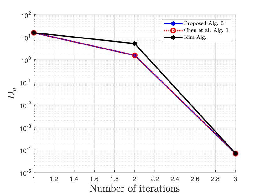
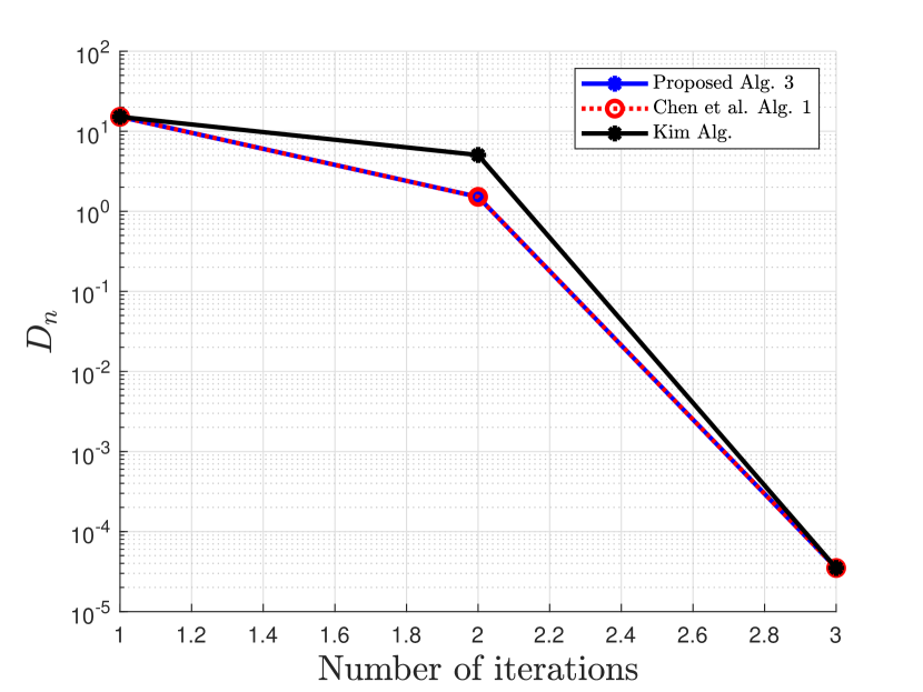
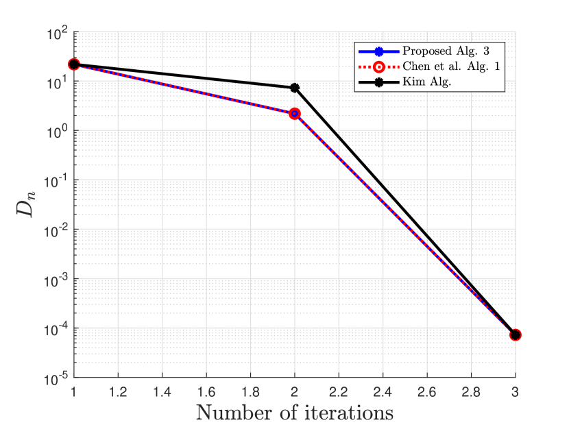
Example 5.1.

First, we compare our proposed 2-Step Inertial Proximal Method of Multipliers in Algorithm 3 with the methods in [20, 35] using the following basis pursuit problem:

\displaystyle\left\{\begin{array}[]{ll}&\min\limits_{x\in\mathbb{R}^{N}}\|u\|_{1}\\ &{\rm subject\leavevmode\nobreak\ to}\leavevmode\nobreak\ \leavevmode\nobreak\ Au=b,\end{array}\right.

(96)

where $A\in\mathbb{R}^{M\times N}$ and $b\in\mathbb{R}^{M}$ . In our experiment, we consider $N=200,500$ and $M=50,100$ and $A$ is randomly generated. A true sparse $u^{*}$ is randomly generated followed by a thresholding to sparsify nonzero elements, and $b$ is then given by $Au^{*}$ . We run 100 iterations of the proximal method of multipliers and its variants with initial $x_{0}=\textbf{0}$ . Since the $u_{n+1}$ -update does not have a closed form, we used a sufficient number of iterations to solve the $u_{n+1}$ -update using the strongly convex version of FISTA [12] in [16, Theorem 4.10]. The stopping criterion for this example is $D_{n}:=||y_{n}-x_{n+1}||_{2}\leq\epsilon$ , where $\epsilon=10^{-4}$ . The parameter used are provided in Table 1

Table 1: Methods Parameters for Example 5.1

Proposed Alg. 3	$\displaystyle\lambda_{1}=10^{-4}$	$\displaystyle\theta=0.1$	$\displaystyle\delta=-0.14412$
Chen et al. Alg.	$\displaystyle\lambda_{1}=10^{-4}$	$\displaystyle\theta=0.1$	$\displaystyle\delta=0$
Kim Alg.	$\displaystyle\lambda_{1}=10^{-4}$

Table 2: Example 5.1 comparison for different

N

and

M

	$(N,M)=(200,50)$		$(N,M)=(200,100)$
	No. of Iter.	CPU Time	No. of Iter.	CPU Time
Proposed Alg. 3	3	$4.3561\times 10^{-3}$	3	$4.1955\times 10^{-3}$
Chen et al. Alg. 1	3	$5.8181\times 10^{-3}$	3	$4.7572\times 10^{-3}$
Kim Alg.	3	$5.0265\times 10^{-3}$	3	$5.5091\times 10^{-3}$
	$(N,M)=(500,50)$		$(N,M)=(500,100)$
	No. of Iter.	CPU Time	No. of Iter.	CPU Time
Proposed Alg. 3	3	$2.7343\times 10^{-2}$	3	$3.0797\times 10^{-2}$
Chen et al. Alg. 1	3	$3.0817\times 10^{-2}$	3	$3.1057\times 10^{-2}$
Kim Alg.	3	$2.8120\times 10^{-2}$	3	$3.8054\times 10^{-2}$

Refer to caption — Figure 1: Example 5.1: $(N,M)=(200,50)$

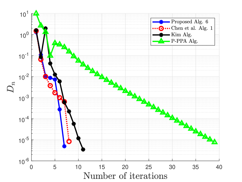
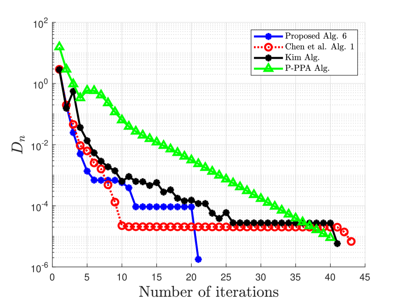
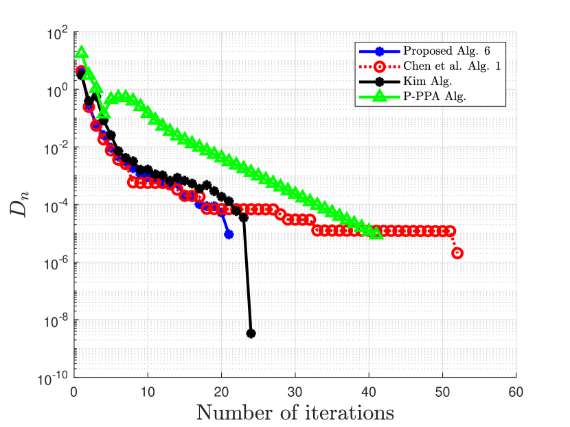
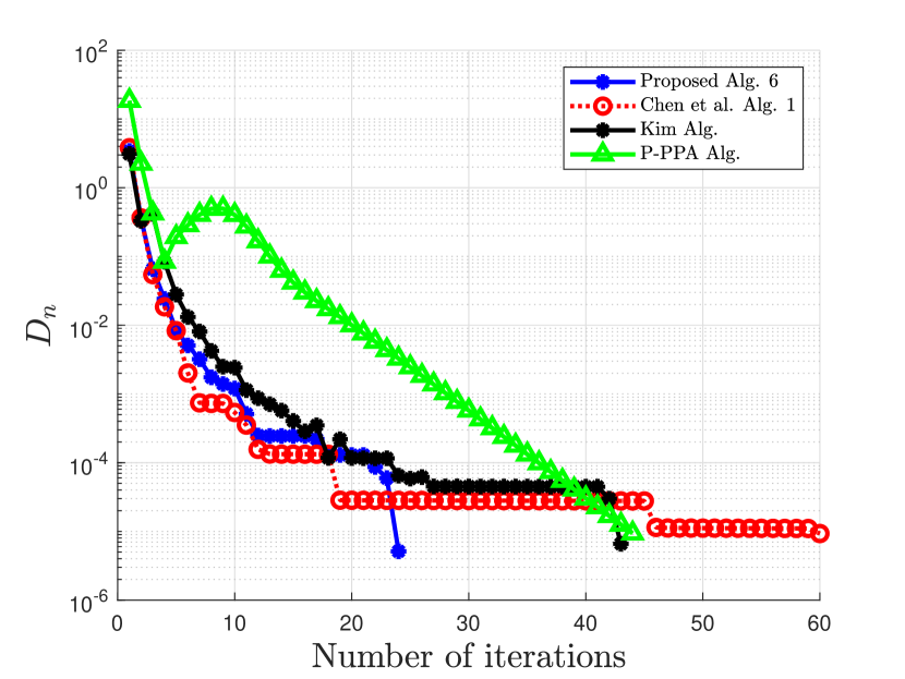
Example 5.2.

In this example, we apply our proposed 2-Step Inertial ADMM (Algorithm 6) to the problem

\displaystyle\left\{\begin{array}[]{ll}&\min\limits_{x\in\mathbb{R}^{N}}\max\limits_{z\in\mathbb{R}^{M}}\frac{1}{2}\|Fx-b\|^{2}+\gamma\|z\|_{1}\\ &s.t.Dx-z=0\end{array}\right.

(99)

where $\gamma>0$ and compare with the methods in [9, 20, 35]. The problem (99) is associated with the total-variation-regularized least squares problem

\min_{x\in\mathbb{R}^{N}}\frac{1}{2}\|Fx-b\|^{2}+\gamma\|Dx\|_{1},

(100)

where $F\in\mathbb{R}^{p\times N},b\in\mathbb{R}^{p}$ , and a matrix $D\in\mathbb{R}^{M\times N}$ is given as

\displaystyle D=\left(\begin{array}[]{ccccccc}-1&1&0&0&\ldots&0&\\ 0&1&-1&0&\ldots&0&\\ \vdots&\ddots&\ddots&\ddots&\ddots&\vdots&\\ \vdots&\ddots&0&1&-1&0&\\ 0&\ldots&\ldots&0&1&-1&\end{array}\right)

Take $f(x):=\frac{1}{2}\|Fx-b\|^{2},g(z):=\gamma\|z\|_{1},A=D,B=-I$ and $c=0$ in (84), our 2-Step Inertial ADMM 6 reduces to:

Algorithm 7 2-Step Inertial ADMM

1:Choose parameters

\delta

and

\theta

satisfying condition (18). Choose

x_{0}\in\mathbb{R}^{N},z_{0}\in\mathbb{R}^{M},\hat{v}_{0}\in\mathbb{R}^{M},\lambda>0

. Set

n=0.

2:Compute as follows:

\displaystyle\left\{\begin{array}[]{ll}&x_{n+1}={\rm arg}\min\limits_{x\in\mathbb{R}^{N}}\Big{\{}\frac{1}{2}\|Fx-b\|^{2}+\langle\hat{v}_{n},Dx-z_{n}\rangle+\frac{\lambda}{2}\|Dx-z_{n}\|^{2}\Big{\}}\\ &=(F^{T}F+\lambda D^{T}D)^{-1}(D^{T}(\lambda z_{n}-\hat{v}_{n})+F^{T}b),\\ &\hat{\eta}_{n}=\hat{v}_{n},n=0,1,\\ &\hat{\eta}_{n}=\hat{v}_{n}+\theta(\hat{v}_{n}-\hat{v}_{n-1}+\lambda D(x_{n+1}-x_{n}))+\delta(\hat{v}_{n-1}-\hat{v}_{n-2}+\lambda D(x_{n}-x_{n-1}))\\ &n=2,3,\ldots\\ &z_{n+1}={\rm arg}\min\limits_{z\in\mathbb{R}^{M}}\Big{\{}\gamma\|z\|_{1}+\langle\hat{\eta}_{n},Dx_{n+1}-z\rangle+\frac{\lambda}{2}\|Dx_{n+1}-z\|^{2}\Big{\}}\\ &=S_{\frac{\gamma}{\lambda}}\Big{(}Dx_{n+1}+\frac{1}{\lambda}\hat{\eta}_{n}\Big{)}\\ &\hat{v}_{n+1}=\hat{\eta}_{n}+\lambda(Dx_{n+1}-z_{n+1}),\end{array}\right.

(110)

3:Set

n\leftarrow n+1

, and go to 2.

where $S_{\tau}(z):=\max\{|z|-\tau,0\}\odot{\rm sign}(z)$ is the soft-thresholding operator, with the element-wise absolute value, maximum and multiplication operators, $|.|,\max\{.,.\}$ and $\odot$ , respectively.

In this numerical test, we consider different cases for the choices of $N$ , $M$ , and $p$ . A true vector $x^{*}$ is constructed such that a vector $Dx^{*}$ has few nonzero elements. A matrix $F$ is randomly generated and a noisy vector $b$ is generated by adding randomly generated (noise) vector to $Fx^{*}$ .

Case 1: $N=100$ , $M=99$ , and $p=5$
Case 2: $N=200$ , $M=199$ , and $p=10$
Case 3: $N=300$ , $M=299$ , and $p=20$
Case 4: $N=400$ , $M=399$ , and $p=40$

The stopping criterion for this example is $D_{n}\leq\epsilon$ , where $\epsilon=10^{-5}$ . The parameter used are provided in Table 3.

Table 3: Methods Parameters for Example 5.2

Proposed Alg. 3	$\displaystyle\lambda_{1}=0.1$	$\displaystyle\theta=0.1$	$\displaystyle\delta=-10^{-3}$	$\displaystyle\gamma=0.01$
	$D_{n}:=\|\|Dx_{n}-z_{n}\|\|_{2}^{2}$
Chen et al. Alg.	$\displaystyle\lambda_{1}=0.1$	$\displaystyle\theta=0.1$	$\displaystyle\delta=0$	$\displaystyle\gamma=0.01$
	$D_{n}:=\|\|Dx_{n}-z_{n}\|\|_{2}^{2}$
Kim Alg.	$\displaystyle\lambda_{1}=0.1$	$\displaystyle\gamma=0.01$	$D_{n}:=\|\|Dx_{n}-z_{n}\|\|_{2}^{2}$
P-PPA Alg.	$\displaystyle s=10$	$\displaystyle\rho=6$	$\displaystyle\varepsilon=1.5$	$\displaystyle\tau=1.5$
	$\displaystyle\sigma=\frac{1.1}{s}$	$\displaystyle\mu=0.1\|\|F^{T}b\|\|_{\infty}$	$D_{n}:=\|\|y_{n+1}-y_{n}\|\|_{2}$

Table 4: Example 5.1 comparison for different cases

	Case 1		Case 2
	No. of Iter.	CPU Time	No. of Iter.	CPU Time
Proposed Alg. 6	7	$1.9990\times 10^{-4}$	21	$1.2536\times 10^{-3}$
Chen et al. Alg. 1	8	$1.9240\times 10^{-4}$	43	$2.6423\times 10^{-3}$
Kim Alg.	11	$2.9860\times 10^{-4}$	41	$2.3246\times 10^{-3}$
P-PPA Alg.	39	$1.2939\times 10^{-3}$	40	$2.6799\times 10^{-3}$
	Case 3		Case 4
	No. of Iter.	CPU Time	No. of Iter.	CPU Time
Proposed Alg. 3	21	$2.2213\times 10^{-3}$	24	$7.2828\times 10^{-3}$
Chen et al. Alg. 1	52	$6.4371\times 10^{-3}$	60	$2.3097\times 10^{-2}$
Kim Alg.	24	$2.7002\times 10^{-3}$	43	$1.5199\times 10^{-2}$
P-PPA Alg.	41	$3.5834\times 10^{-3}$	44	$1.2796\times 10^{-2}$

Remark 5.3.

From the above numerical Examples 5.1 and 5.2, we give the following remarks.

(1).

Noting from Figures 2 - 8 and Tables 2 and 4, our proposed Algorithms are clearly easy to implement, efficiency and accurate.
(2).

Clearly from the numerical Example 5.2, our proposed Algorithm 6 outperforms the algorithm proposed by Chen et al. in [20], the algorithm proposed by Kim in [35], and the algorithm proposed by Bai et al. in [9] with respect to the number of iterations and the CPU time. The proposed algorithm 3 also competes favorably with Chen et al. Alg. 1 in [20] and that of Kim in [35] for the case of Example 5.1.

6 Conclusion

We have introduced in this paper, a two-step inertial proximal point algorithm for monotone inclusion problem in Hilbert spaces. Weak convergence of the sequence of iterates are obtained under standard conditions and non-asymptotic $\textit{O}(1/n)$ rate of convergence in the ergodic sense given. We support the theoretical analysis of our method with numerical illustrations derived from basis pursuit problem and numerical implementation of two-step inertial ADMM. Preliminary numerical results show that our proposed method is competitive and outperforms some related and recent proximal point algorithms in the literature. Part of our future projects is to study two-step inertial proximal point algorithm with corrected term for the monotone inclusion considered in this paper.

Acknowledgements

The authors are grateful to the associate editor and the two anonymous referees for their insightful comments and suggestions which have improved greatly on the earlier version of the paper.

References

[1] Aluffi-Pentini F, Parisi V., Zirilli F. Algorithm 617. DAFNE: a differential-equations algorithm for nonlinear equations. ACM Trans. Math. Software 10 (1984), 317-324.
[2] Alvarez F. On the minimizing property of a second order dissipative system in Hilbert spaces. SIAM J. Control Optim. 38 (2000), 1102–1119.
[3] Alvarez F., Attouch H. An inertial proximal method for maximal monotone operators via discretization of a nonlinear oscillator with damping. Set-Valued Anal. 9 (2001), 3–11.
[4] Alvarez F. Weak convergence of a relaxed and inertial hybrid projection-proximal point algorithm for maximal monotone operators in Hilbert space. SIAM J. Optim. 14 (2004), 773–782.
[5] Antipin A. S. Minimization of convex functions on convex sets by means of differential equations. Differentsial’nye Uravneniya 30 (1994), 1475-1486, 1652; translation in Differential Equations 30 (1994), 1365–1375.
[6] Attouch H., Cabot, A. Convergence rate of a relaxed inertial proximal algorithm for convex minimization. Optimization 69 (2020), 1281-1312.
[7] Attouch H., Peypouquet J., Redont P. A dynamical approach to an inertial forward-backward algorithm for convex minimization. SIAM J. Optim. 24 (2014), 232-256.
[8] Aujol J.-F. , Dossal C., Rondepierre A. Optimal Convergence Rates for Nesterov Acceleration. SIAM J. Optim. 29 (2019), 3131-3153.
[9] Bai, J., Zhang, H., Li, J. A parameterized proximal point algorithm for separable convex optimization. Optim. Lett. 12 (2018), 1589-1608.
[10] Bai, J., Hager, W., Zhang, H. An inexact accelerated stochastic ADMM for separable composite convex optimization. Comput. Optim. Appl. 81 (2022), 479-518.
[11] Bai, J., Han, D., Sun, H., Zhang, H. Convergence analysis of an inexact accelerated stochastic ADMM with larger stepsizes. CSIAM Trans. Appl. Math. To appear, arXiv:2103.16154v2, (2022).
[12] A. Beck and M. Teboulle; A fast iterative shrinkage-thresholding algorithm for linear inverse problems, SIAM J. Imaging Sci. 2 (1) (2009), 183-202.
[13] Bruck R. E., Jr. Asymptotic convergence of nonlinear contraction semigroups in Hilbert space. J. Functional Analysis 18 (1975), 15–26.
[14] Bot R. I., Csetnek E. R., Hendrich C. Inertial Douglas-Rachford splitting for monotone inclusion problems. Appl. Math. Comput. 256 (2015), 472–487.
[15] Bot R. I., Csetnek E. R. An inertial alternating direction method of multipliers. Minimax Theory Appl. 1 (2016), 29-49.
[16] Chambolle, A., Pock, T. An introduction to continuous optimization for imaging. Acta Numer. 25, 161–319 (2016).
[17] Chambolle, A., Pock, T. On the ergodic convergence rates of a first-order primal-dual algorithm. Math. Program. 159 (2016), Ser. A, 253–287.
[18] A. Chambolle, T. Pock; A first-order primal-dual algorithm for convex problems with applications to imaging. J. Math. Imaging and Vision 40(1) (2011), 120-145.
[19] A. Chambolle and T. Pock; On the ergodic convergence rates of a first-order primal–dual algorithm, Math. Program. 159 (2016), 253-287.
[20] C. Chen, S. Ma, and J. Yang; A general inertial proximal point algorithm for mixed variational inequality problem, SIAM J. Optim. 25 (2015), 2120–2142.
[21] Cholamjiak P., Thong D.V., Cho Y.J. A novel inertial projection and contraction method for solving pseudomonotone variational inequality problems. Acta Appl. Math. 169 (2020), 217-245.
[22] Combettes, P. L., Glaudin, L. E. Quasi-nonexpansive iterations on the affine hull of orbits: from Mann’s mean value algorithm to inertial methods. SIAM J. Optim. 27 (2017), 2356-2380.
[23] Corman, E., Yuan, X. M. A generalized proximal point algorithm and its convergence rate. SIAM J. Optim. 24 (2014), 1614-1638.
[24] Davis, D., Yin W. Faster convergence rates of relaxed Peaceman-Rachford and ADMM under regularity assumptions. Math. Oper. Res. 42 (2017), 783-805.
[25] Dong, Q.L., Huang, J.Z., Li, X.H., Cho, Y. J., Rassias, Th. M. MiKM: multi-step inertial Krasnosel’skii–Mann algorithm and its applications. J. Global Optim. 73, 801–824 (2019).
[26] Dong Q. L., Jiang D., Cholamjiak P., Shehu Y. A strong convergence result involving an inertial forward-backward algorithm for monotone inclusions. J. Fixed Point Theory Appl. 19 (2017), 3097-3118.
[27] J. Douglas and H.H. Rachford; On the numerical solution of heat conduction problems in two or three space variables, Trans. Amer. Math. Soc. 82 (1956), 421-439.
[28] Eckstein, J., Bertsekas, D.P. On the Douglas-Rachford splitting method and the proximal point algorithm for maximal monotone operators. Math. Program. 55 (1992), Ser. A, 293-318.
[29] Esser, E., Zhang, X., Chan, T. A general framework for a class of first order primal-dual algorithms for convex optimization in imaging science. SIAM J. Imaging Sci. 3(4), 1015–46 (2010).
[30] Gabay, D., Mercier, B. A dual algorithm for the solution of nonlinear variational problems via finite element approximation. Comput. Math. Appl. 2 (1976), 17-40.
[31] Glowinski, R., Marrocco, A. Sur l’approximation, par élḿents finis d’ordre un, et la résolution, par pénalisation-dualité, d’une classe de problèmes de Dirichlet non linéaires. (French) Rev. Française Automat. Informat. Recherche Opérationnelle Sér. Rouge Anal. Numér. 9 (1975), no. R-2, 41-76.
[32] G $\ddot{u}$ ler, O. New proximal point algorithms for convex minimization. SIAM J. Optim. 2 (1992), 649-664.
[33] Hestenes, M. R. Multiplier and gradient methods. J. Optim. Theory Appl. 4 (1969), 303-320.
[34] He, B., Yuan, X. Convergence analysis of primal-dual algorithms for a saddle-point problem: from contraction perspective. SIAM J. Imaging Sci. 5(1), 119–49 (2012).
[35] Kim, D., Accelerated proximal point method for maximally monotone operators. Math. Program. 190 (2021), 57–87.
[36] J. Liang, Convergence rates of first-order operator splitting methods. PhD thesis, Normandie Université; GREYC CNRS UMR 6072, 2016.
[37] P.L. Lions and B. Mercier; Splitting algorithms for the sum of two nonlinear operators, SIAM J. Numer. Anal. 16 (1979), 964-979.
[38] Lorenz, D. A., Pock, T. An inertial forward-backward algorithm for monotone inclusions. J. Math. Imaging Vision 51 (2015), 311-325.
[39] Ma, F., Ni, M. A class of customized proximal point algorithms for linearly constrained convex optimization. Comp. Appl. Math. 37 (2018), 896-911.
[40] Maingé, P. E., Merabet, N. A new inertial-type hybrid projection-proximal algorithm for monotone inclusions. Appl. Math. Comput. 215 (2010), 3149-3162.
[41] Martinet, B. Régularisation d’inéquations variationnelles par approximations successives. (French) Rev. Française Informat. Recherche Opérationnelle 4 (1970), Sér. R-3, 154–158.
[42] Tao, M., Yuan, X. On the optimal linear convergence rate of a generalized proximal point algorithm. J. Sci. Comput. 74 (2018), 826-850.
[43] Moreau, J. J. Proximité et dualité dans un espace Hilbertien. (French) Bull. Soc. Math. France 93 (1965), 273-299.
[44] Moudafi, A., Elisabeth, E. An approximate inertial proximal method using the enlargement of a maximal monotone operator. Int. J. Pure Appl. Math. 5 (2003), 283-299.
[45] B.T. Polyak, Some methods of speeding up the convergence of iterates methods, U.S.S.R Comput. Math. Phys., 4 (5) (1964), 1-17.
[46] B. T. Polyak, Introduction to optimization. New York, Optimization Software, Publications Division, 1987.
[47] C. Poon, J. Liang, Trajectory of Alternating Direction Method of Multipliers and Adaptive Acceleration, In Advances In Neural Information Processing Systems (2019).
[48] C. Poon, J. Liang, Geometry of First-Order Methods and Adaptive Acceleration, arXiv:2003.03910.
[49] Powell, M. J. D. A method for nonlinear constraints in minimization problems. 1969 Optimization (Sympos., Univ. Keele, Keele, 1968) pp. 283–298 Academic Press, London.
[50] Rockafellar, R. T. Monotone operators and the proximal point algorithm. SIAM J. Control Optim. 14 (1976), 877–898.
[51] R. T. Rockafellar; Monotone operators and the proximal point algorithm, SIAM J. Control. Optim. 14 (1976) 877-898.

	$\displaystyle\\|(1+a)x-(a-b)y-bz\\|^{2}$	$\displaystyle=$	$\displaystyle(1+a)\\|x\\|^{2}-(a-b)\\|y\\|^{2}-b\\|z\\|^{2}+(1+a)(a-b)\\|x-y\\|^{2}$
			$\displaystyle+b(1+a)\\|x-z\\|^{2}-b(a-b)\\|y-z\\|^{2}.$

$\displaystyle\\|y_{n}-x^{*}\\|^{2}$	$\displaystyle=$	$\displaystyle\\|(1+\theta)(x_{n}-x^{})-(\theta-\delta)(x_{n-1}-x^{})-\delta(x_{n-2}-x^{*})\\|^{2}$	(22)
	$\displaystyle=$	$\displaystyle(1+\theta)\\|x_{n}-x^{}\\|^{2}-(\theta-\delta)\\|x_{n-1}-x^{}\\|^{2}-\delta\\|x_{n-2}-x^{*}\\|^{2}$
		$\displaystyle+(1+\theta)(\theta-\delta)\\|x_{n}-x_{n-1}\\|^{2}+\delta(1+\theta)\\|x_{n}-x_{n-2}\\|^{2}$
		$\displaystyle-\delta(\theta-\delta)\\|x_{n-1}-x_{n-2}\\|^{2}.$

$\displaystyle\\|x_{n+1}-y_{n}\\|^{2}$	$\displaystyle=$	$\displaystyle\\|x_{n+1}-(x_{n}+\theta(x_{n}-x_{n-1})+\delta(x_{n-1}-x_{n-2}))\\|^{2}$	(26)
	$\displaystyle=$	$\displaystyle\\|x_{n+1}-x_{n}-\theta(x_{n}-x_{n-1})-\delta(x_{n-1}-x_{n-2})\\|^{2}$
	$\displaystyle=$	$\displaystyle\\|x_{n+1}-x_{n}\\|^{2}-2\theta\langle x_{n+1}-x_{n},x_{n}-x_{n-1}\rangle$
		$\displaystyle-2\delta\langle x_{n+1}-x_{n},x_{n-1}-x_{n-2}\rangle+\theta^{2}\\|x_{n}-x_{n-1}\\|^{2}$
		$\displaystyle+2\delta\theta\langle x_{n}-x_{n-1},x_{n-1}-x_{n-2}\rangle+\delta^{2}\\|x_{n-1}-x_{n-2}\\|^{2}$
	$\displaystyle\geq$	$\displaystyle\\|x_{n+1}-x_{n}\\|^{2}-2\theta\\|x_{n+1}-x_{n}\\|\\|x_{n}-x_{n-1}\\|$
		$\displaystyle-2\|\delta\|\\|x_{n+1}-x_{n}\\|\\|x_{n-1}-x_{n-2}\\|+\theta^{2}\\|x_{n}-x_{n-1}\\|^{2}$
		$\displaystyle-2\|\delta\|\theta\\|x_{n}-x_{n-1}\\|\\|x_{n-1}-x_{n-2}\\|+\delta^{2}\\|x_{n-1}-x_{n-2}\\|^{2}$
	$\displaystyle\geq$	$\displaystyle\\|x_{n+1}-x_{n}\\|^{2}-\theta\\|x_{n+1}-x_{n}\\|^{2}-\theta\\|x_{n}-x_{n-1}\\|^{2}$
		$\displaystyle-\|\delta\|\\|x_{n+1}-x_{n}\\|^{2}-\|\delta\|\\|x_{n-1}-x_{n-2}\\|^{2}+\theta^{2}\\|x_{n}-x_{n-1}\\|^{2}$
		$\displaystyle-\|\delta\|\theta\\|x_{n}-x_{n-1}\\|^{2}-\|\delta\|\theta\\|x_{n-1}-x_{n-2}\\|^{2}+\delta^{2}\\|x_{n-1}-x_{n-2}\\|^{2}$
	$\displaystyle=$	$\displaystyle(1-\|\delta\|-\theta)\\|x_{n+1}-x_{n}\\|^{2}+(\theta^{2}-\theta-\|\delta\|\theta)\\|x_{n}-x_{n-1}\\|^{2}$
		$\displaystyle+(\delta^{2}-\|\delta\|-\|\delta\|\theta)\\|x_{n-1}-x_{n-2}\\|^{2}.$

$\displaystyle\\|x_{n+1}-x^{*}\\|^{2}$	$\displaystyle=$	$\displaystyle\\|J_{\lambda}^{A}(y_{n})-x^{*}\\|^{2}$	(27)
	$\displaystyle=$	$\displaystyle\\|J_{\lambda}^{A}(y_{n})-J_{\lambda}^{A}(x^{*})\\|^{2}$
	$\displaystyle\leq$	$\displaystyle\\|y_{n}-x^{*}\\|^{2}-\\|J_{\lambda}^{A}(y_{n})-y_{n}\\|^{2}$
	$\displaystyle=$	$\displaystyle\\|y_{n}-x^{*}\\|^{2}-\\|x_{n+1}-y_{n}\\|^{2}$
	$\displaystyle\leq$	$\displaystyle(1+\theta)\\|x_{n}-x^{}\\|^{2}-(\theta-\delta)\\|x_{n-1}-x^{}\\|^{2}-\delta\\|x_{n-2}-x^{*}\\|^{2}$
		$\displaystyle+(1+\theta)(\theta-\delta)\\|x_{n}-x_{n-1}\\|^{2}+\delta(1+\theta)\\|x_{n}-x_{n-2}\\|^{2}$
		$\displaystyle-\delta(\theta-\delta)\\|x_{n-1}-x_{n-2}\\|^{2}-(1-\|\delta\|-\theta)\\|x_{n+1}-x_{n}\\|^{2}$
		$\displaystyle-(\theta^{2}-\theta-\|\delta\|\theta)\\|x_{n}-x_{n-1}\\|^{2}-(\delta^{2}-\|\delta\|-\|\delta\|\theta)\\|x_{n-1}-x_{n-2}\\|^{2}$
	$\displaystyle=$	$\displaystyle(1+\theta)\\|x_{n}-x^{}\\|^{2}-(\theta-\delta)\\|x_{n-1}-x^{}\\|^{2}-\delta\\|x_{n-2}-x^{*}\\|^{2}$
		$\displaystyle+\Big{(}(1+\theta)(\theta-\delta)-(\theta^{2}-\theta-\|\delta\|\theta)\Big{)}\\|x_{n}-x_{n-1}\\|^{2}$
		$\displaystyle+\delta(1+\theta)\\|x_{n}-x_{n-2}\\|^{2}-(1-\|\delta\|-\theta)\\|x_{n+1}-x_{n}\\|^{2}$
		$\displaystyle-\Big{(}\delta(\theta-\delta)+(\delta^{2}-\|\delta\|-\|\delta\|\theta)\Big{)}\\|x_{n-1}-x_{n-2}\\|^{2}$
	$\displaystyle=$	$\displaystyle(1+\theta)\\|x_{n}-x^{}\\|^{2}-(\theta-\delta)\\|x_{n-1}-x^{}\\|^{2}-\delta\\|x_{n-2}-x^{*}\\|^{2}$
		$\displaystyle+(2\theta-\delta-\delta\theta+\|\delta\|\theta)\\|x_{n}-x_{n-1}\\|^{2}+\delta(1+\theta)\\|x_{n}-x_{n-2}\\|^{2}$
		$\displaystyle-(1-\|\delta\|-\theta)\\|x_{n+1}-x_{n}\\|^{2}+(\|\delta\|+\|\delta\|\theta-\delta\theta)\\|x_{n-1}-x_{n-2}\\|^{2}$
	$\displaystyle\leq$	$\displaystyle(1+\theta)\\|x_{n}-x^{}\\|^{2}-(\theta-\delta)\\|x_{n-1}-x^{}\\|^{2}-\delta\\|x_{n-2}-x^{*}\\|^{2}$
		$\displaystyle+(2\theta-\delta-\delta\theta+\|\delta\|\theta)\\|x_{n}-x_{n-1}\\|^{2}-(1-\|\delta\|-\theta)\\|x_{n+1}-x_{n}\\|^{2}$
		$\displaystyle+(\|\delta\|+\|\delta\|\theta-\delta\theta)\\|x_{n-1}-x_{n-2}\\|^{2}.$

	$\displaystyle\\|x_{n+1}-x^{}\\|^{2}-\theta\\|x_{n}-x^{}\\|^{2}-\delta\\|x_{n-1}-x^{*}\\|^{2}+(1-\|\delta\|-\theta)\\|x_{n+1}-x_{n}\\|^{2}$	(28)
$\displaystyle\leq$	$\displaystyle\\|x_{n}-x^{}\\|^{2}-\theta\\|x_{n-1}-x^{}\\|^{2}-\delta\\|x_{n-2}-x^{*}\\|^{2}$
	$\displaystyle+(1-\|\delta\|-\theta)\\|x_{n}-x_{n-1}\\|^{2}+(3\theta-1+(1+\theta)(\|\delta\|-\delta))\\|x_{n}-x_{n-1}\\|^{2}$
	$\displaystyle+(\|\delta\|+\|\delta\|\theta-\delta\theta)\\|x_{n-1}-x_{n-2}\\|^{2}.$