Convex Decreasing Algorithms: Distributed Synthesis and Finite-time Termination in Higher Dimension
Abstract
We introduce a general mathematical framework for distributed algorithms, and a monotonicity property frequently satisfied in application. These properties are leveraged to provide finite-time guarantees for converging algorithms, suited for use in the absence of a central authority. A central application is to consensus algorithms in higher dimension. These pursuits motivate a new peer to peer convex hull algorithm which we demonstrate to be an instantiation of the described theory. To address the diversity of convex sets and the potential computation and communication costs of knowing such sets in high dimension, a lightweight norm based stopping criteria is developed. More explicitly, we give a distributed algorithm that terminates in finite time when applied to consensus problems in higher dimensions and guarantees the convergence of the consensus algorithm in norm, within any given tolerance. Applications to consensus least squared estimation and distributed function determination are developed. The practical utility of the algorithm is illustrated through MATLAB simulations.
I Introduction
Recent advancements in the field of intelligent communication technologies and ad-hoc wireless sensor networks for monitoring and control of multi-agent systems have necessitated design of algorithms to assert global information without the complete knowledge of the system. The task of obtaining the global information is often accomplished via a class of algorithms that employ strategies of achieving consensus. In a consensus algorithm, agents iteratively and in a distributed manner agree on a common state. The ideas of distributed consensus algorithms can be traced back to the seminal works, see [1, 2, 3, 4]. Recent works on consensus algorithms are focused on designing protocols to drive agents to the average of their initial states, see [5, 6, 7, 8]. These protocols were designed for cases where the state of each agent is a scalar value. However, increasing storage and computation capabilities of modern day sensor interfacing technologies have motivated large-scale applications, examples of which include distributed machine learning, see [9], multi-agent control and co-ordination, see [10, 11], distributed optimization problems, see [12, 13], distributed sensor localization, see [14]. In order to meet the requirements of such applications there is need of distributed consensus algorithms that allow for vector states. [15] presents such a higher dimensional consensus protocol. The framework in [15] is based on a leader-follower architecture with the agents being partitioned between anchors and sensors. Anchors are agents with fixed states behaving as leaders in the algorithm, while the sensors change their state by taking a convex combination of their state with the neighboring nodes’ states.
Cyber physical systems such as electrical power networks need to accommodate for large number of states for crucial applications such as state-estimations, optimal dispatch, and demand response for ancillary services. [16] formulates the distributed apportioning problem using consensus protocols where only a single state is shared for each protocol. A similar situation involving higher dimensional states arises in distributed resource allocation problems where a fixed amount of resource is required to be apportioned among all participating agents in a network and a convex cost associated with the each resource is to be distributively minimized. The method used to solve the above resource allocation problem involves a higher dimensional consensus protocol (see [17]).
Other applications where accommodating higher dimensional data is required are distributed optimization and their applications to deep neural networks such as in the case of diffusion learning where local agents perform model training using local datasets in parallel, for example see [18], where after the completion of the training process, model parameters are then shared with the neighboring nodes allowing for faster dissemination of the model parameters. This method also allows for asynchronous learning, where different agents learn with models of different parameters at every iteration. Recent frameworks for unsupervised learning such as Generative Adversarial Networks (GANs) where the objective is to train learning models to be robust against adversarial attacks (see [19]). [20] propose methods for scaling adversarial training and learning to large datasets performed on a distributed setup where each agent trains a discriminator model on a local training data and a shared generator model is trained based on the feedback received from the discriminator models of the different agents. These applications need sharing of a high dimensional parameter vector, usually of the order of . Applications such as spectrum sensing in Ad hoc cognitive radio networks, see [21], distributed detection of malicious attacks in finite-time consensus networks [22] and control of autonomous agents like unmanned aerial vehicles (UAVs) for search and survey operations, see [10] also depend on implementing higher dimensional consensus protocols.
Termination of consensus algorithms in finite time provides an advantage of getting an approximate consensus while saving valuable computation and communication resources. For the scalar average consensus protocols discussed earlier, the authors in [23, 24] have proposed such a finite time stopping criteria utilizing two additional states namely the global maximum and global minimum over the network. This allows each agent to distributively detect the convergence to the (approximate) average and terminate further computations. The works in [25, 26] generalize this result to the cases of dynamic interconnection topology and communication delays. The authors in [27] present a method based on the minimal polynomial associated with the weight matrix in the state update iterations to achieve the consensus value in a finite number of iterations. However, to calculate the coefficients of the minimal polynomial each node has to run (total number of agents) different linear iterations each for at least time-steps.
The protocol developed here is based on a new geometric insight into the behavior of push-sum or ratio consensus algorithms that is of independent interest. We prove that many popular consensus algorithms fit into a general class of algorithms which we call “convex decreasing”. We demonstrate that convex decreasing consensus algorithms satisfy monotone convergence properties, which we leverage to give guarantees on network configurations. That is, if it can be determined that all nodes of convex decreasing consensus algorithm belongs to a convex set, then all nodes of the algorithm will remain in said convex set. We develop distributed stopping criteria based on this geometric insight.
Centralized algorithms for finding the convex hull of a finite set of points in a plane have been long proposed. Such algorithms have the worst-case running time of , which is also the best achievable performance for obtaining the ordered hull (see [28]). However, with the recent advancements in distributed multi-agent systems, the problem of estimating the convex hull in a distributed manner, in the absence of a centralized entity, has become important. To this regard, distributed algorithms to estimate convex hull have been proposed in the literature for applications such as in classification problems, locational region estimation and formation control to name a few. In classification problems, [29, 30] have proposed an one-class scaled distributed convex hull algorithm where the geometric structure of the convex hull is used to model the boundary of the target class defining the one-class. However an approximation of the convex hull in the original large dimensional space by means of randomly projected decisions on 2-D spaces results in a residual error when applied to finite time applications as analyzed in [31]. In order to obtain the convex hull of the feature space (kernel space) by communicating the extremities, [32] employed a quadratic programming approach. However, the computational complexity of the proposed solution is limiting when extended to higher dimensions. [33] proposed a convex hull algorithm, but require the assumption that the feature space is generated from a Gaussian mixture model and thus is limited to applications of a special class of support vector machines. A difference in paradigm between the convex hull estimation pursued here and the literature on distributed programming for computation of convex hulls, is that the current article constructs a protocol that can be implemented in a plug and play manner in the absence of a central authority or knowledge of the network.
The problem of computing a specified function of the sensor measurements is common in wireless sensor networks, see [34], [35]. The setup in [34] focuses on the problem of determining an arbitrary function of the sensor measurements from a specified sink node. The article studies the maximum rate at which the function can be calculated and communicated to the sink node. The article provides a characterization of the achievable rates for thee different classes of functions. The authors in [35] proposed a method to calculate any arbitrary function in networks utilizing a linear iteration. The authors show that the proposed method can be modeled as a dynamical system. Based on the structured system observability approach it is shown that the linear iterations can determine any specified function of the initial values of the nodes after observing the evolution of the agent values for a large but finite time-steps. However, the method is based on forming observability matrices for all agents in the network; here the method poses limitations as the size of the network increases leading to a large amount of computation and storage requirement. Further, the linear iterations require doubly-stochastic matrices for the agent state updates. The need of doubly-stochastic matrices makes the method in [35] not applicable to directed networks. In this article we propose a distributed algorithm to determine any arbitrary function of the initial values of the agents, applicable to general connected directed graph topologies. Moreover, the proposed method has a fixed storage requirement and the communication overhead of the proposed method compared to the existing methods is insignificant.
In this article, we present a distributed stopping criteria for the higher dimensional consensus problem. Our first progress in this direction can be found in [36], where we investigated distributed stopping algorithm for the special case of “ratio consensus”. Here we present a general theory of convex monotonicity, and demonstrate that one can apply the distributed termination techniques to any algorithm satisfying this criteria. In particular we show that in popular consensus algorithms (ratio consensus and row stochastic for example), the evolution of the convex hull of network states (in any dimension) indexed by time form a nested sequence of convex sets. This motivates an algorithm for distributively computing the convex hull within a time that scales linear with diameter of the network. We further provide a simpler algorithm which guarantees the convergence of consensus algorithm in norm, within any given tolerance.
Statement of contribution:
-
1.
This article constructs a general mathematical framework for convergence of network algorithms. In particular a notion of monotoniticity satisfied by important consensus algorithms is introduced. We show ratio consensus [5] and row stochastic updating of a network to be examples of “convex decreasing” algorithms.
-
2.
A convex hull algorithm, of independent interest, is developed for distributed determination of the extreme points of a set of vectors in the absence of a central authority. In the context of a distributed convex decreasing algorithm, the hull algorithm can be used by the agents to obtain the convex hull by a fixed time , and thus give guarantees on the state of the convex decreasing algorithm for all times .
-
3.
Feasibility concerns for convex hull computation are addressed for high dimensional data, and an alternative lightweight (in the sense of both computational and communication cost) stopping criterion is given that guarantees finite convergence within an -threshold of consensus with respect to an arbitrary norm.
-
4.
As application of the theory developed, new stopping criteria are developed for consensus based least square estimation as well as distributed function calculation that give the agents convergence guarantees in a peer to peer network.
The rest of the paper is organized as follows. In Section II, the basic definitions needed for subsequent developments are presented. Further, we discuss the setup for the distributed average consensus in higher dimensions (called the vector consensus problem) using ratio consensus. Sections III presents an analysis on the polytopes of the network states generated in the ratio consensus algorithm. Section V establishes a norm-based finite-time termination criterion for the vector consensus problem. Theoretical findings are validated with simulations presented in Section VII followed by conclusions in Section VIII.
II Definitions, and Problem Statement
II-A Definitions and Notations
In this section we present basic notions of graph theory and linear algebra which are essential for the subsequent developments. Detailed description of graph theory and linear algebra notions are available in [37], and [38] respectively. We will also develop a general mathematical framework for consensus algorithms, and introduce a notion of convex monotonicity which will be crucial in the development of stopping criterion for vector consensus.
Definition 1.
(Cardinality of a set) Let be a set. The cardinality of a set denoted by is the number of elements of the set .
Definition 2.
(Directed Graph) A directed graph (denoted as digraph) is a pair where is a set of vertices or nodes and is a set of edges, which are ordered subsets of two distinct elements of . If an edge from to exists then it is denoted as .
Definition 3.
(Path) In a directed graph, a directed path from node to exists if there is a sequence of distinct directed edges of of the form For the rest of the article, a path refers to a directed path.
Definition 4.
(Path Length) The path length, or length of a path is the number of directed edges belonging to the path. By convention, we consider a node to be connected to itself by a path of length zero.
Definition 5.
(Strongly Connected Graph) A directed graph is strongly connected if to every there exists a directed path from node to node .
Definition 6.
(In-Neighborhood) Set of in-neighbors of node is denoted by In this article, we assume for all
Definition 7.
(-In-Neighborhood) For define , and for define to be , so that is the set of nodes from which can be reached in or less steps.
Definition 8.
(Diameter of a Graph) The diameter of a graph is the longest shortest path between any two nodes in the network. We will consider as an upper bound on the diameter of the graph throughout the rest of the article.
Definition 9.
(Network State) For a vector space , a -valued network state is a function , which we denote by .
Definition 10.
(Network Update) A network update on , is a map .
Definition 11.
(Network and Consensus algorithms) A discrete time network algorithm on , is a finite or countably infinite sequence of maps of network updates. When is endowed with a norm , a consensus algorithm is a network algorithm such that for any ,
| (1) |
satisfies,
for all .
We will only consider discrete time network algorithms in this work, a discrete time consensus algorithm will be referred to a consensus algorithm hereafter.
Definition 12.
(Distributed Network Update and Algorithm) A network update , is distributed if satisfying for implies A network algorithm , is distributed if is a distributed network update for every .
For , define to be the restriction of to . Explicitly, for and , . Also, define by
for .
In the following proposition, we gives as alternative formulation of the fact that distributed updates are determined locally.
Proposition II.1.
A network update is distributed if and only if for every , can be expressed as for a function .
Proof.
First suppose a function satisfying exists, and that and satisfy, for , then . Thus . Conversely, assume is a distributed network update and define for . Observe that for , , hence by the definition of a distributed network update
| (2) |
Further by the definition of the function ,
| (3) |
Observe that in the case that the is linear in in the sense that for , then can be represented by a matrix . Conversely, represented by matrices, clearly induce linear .
We will be concerned with linear consensus algorithms, those that can be build from matrix operations. That is when can be represented by a matrix , in the sense that
we will write in place of . Moreover for brevity for exposition, our focus will be on the case that our dynamics are time homogeneous in the sense that .
Definition 13.
(Column Stochastic Matrix) A real matrix is called a column stochastic matrix if for and for
Definition 14.
(Row Stochastic Matrix) A real matrix is called a row stochastic matrix if for and for
Definition 15.
(Irreducible Matrix) A matrix is said to be irreducible if for any , there exist such that , that is, it is possible to reach any state from any other state in a finite number of hops.
Definition 16.
(Primitive Matrix) A non negative matrix is primitive if it is irreducible and has only one eigenvalue of maximum modulus.
As a notational convention, matrices will be written in bold face as above.
Definition 17.
(Convex hull) For a set , the convex hull of is the smallest convex set containing ,
| (4) |
The topological closure of a set , will be denoted
the closure of a convex hull, will be denote .
For we consider to be the convex hull of , when considered as a set of elements of indexed by . More explicitly if we denote the simplex by then for
| (5) |
Definition 18.
(Extreme point) For a convex set define to be an extreme point of , denoted , if for implies . For a general , define .
We will also have use for the following
Definition 19.
For a norm and a set define the diameter of with respect to the norm , .
Definition 20.
Our primary interest is in the case that and for this case we now recall a standard tool from Convex Geometry, the support function of a set, which we can use to give an analytic description of a Convex Decreasing sequence of sets. For , we use the notation , where we use to denote the usual transpose operation.
Definition 21.
(Support function) For a non-empty set , define its support function
Proposition II.2.
Support functions satisfy the following:
-
1.
implies
-
2.
-
3.
-
4.
implies .
-
5.
A sequence of compact sets is convex decreasing if and only if holds for all .
Proof.
Observe that implies, giving (1).
Suppose that and are closed convex sets such that , and take . Then, by the hyperplane seperation theorem [39], there exists such that . This would be a contradiction on , so we must have . For general and , we need only recall from (2) and (3) that and and apply the previous to the closed convex hull to obtain . Thus (4) follows.
We will also have use for a few basic results from Convex Geometry, which we collect bellow.
Lemma II.1.
For convex and compact . For , then
Proof.
The first result is standard (see [39]), its infinite dimensional generalization is the Krein-Milman Theorem (see [40]). For the second result, clearly so that . The reverse inequality follows by fixing and observing , which implies . Since is the smallest convex set containing the proof is complete. ∎
II-B Vector Consensus framework
Here, we extend a key result from [5, 6] where a ratio of two states was maintained to reach average consensus. We consider the network topology to be represented by a directed graph containing nodes and satisfies the following assumptions throughout the rest of the paper.
Assumption 1.
The directed graph representing the agent interconnections is strongly-connected.
Assumption 2.
Let be a primitive column stochastic matrix with digraph with if and only if .
Theorem II.1.
A sequence of matrices defines a scalar consensus algorithm if and only if it defines an vector consensus algorithm.
Proof.
The value of -th node in the -th coordinate after iterations is the application of -iterations to the -th coordinate function evaluated at the -th node, . Hence the theorem follows from the existence of and (dependent on dimension and choice of norm ) such that
with the fact above that the result follows. ∎
Each node maintains three state estimates at time , denoted by (referred as numerator state of node ), (referred as denominator state of node ) and (referred as ratio state of node ). Here is the dimension of each node’s state. Node updates its numerator and denominator states at the discrete iteration according to the following update law:
| (6) | ||||
| (7) |
where, is the set of in-neighbors of node . We will use the notation as shorthand for (6), and observe that . The initial conditions for the numerator vector state and denominator state for any node are:
| (8) |
Node further updates its ratio state as:
| (9) |
Under Assumptions 1, 2 and the initialization in (8), ratio state in (9) is well defined. The next theorem establishes the convergence of the ratio state, which is a direct and simple generalization of the result in [5, 6].
Theorem II.2.
Proof.
In a slightly different framework, we consider the average consensus problem, where each node maintains a single state , for each time , and update its state according to the following update law:
| (10) |
where is a primitive, and row-stochastic, with if and only if . In this case, converges independent of , to for some (see [41]), and in the case that is assumed to be column stochastic as well (see [11]).
III Convex Hull based Finite-Time stopping Criterion
The following theorem shows that consensus algorithms that are convex decreasing converge to the same finite limit at all nodes, and that if one sets an threshold for convergence with an open set about the consensus, the threshold will be met in finite time. Further, when the threshold set is assumed convex, it is proven that if all agents possess a value within the set, their updated values remain within this threshold. In this sense, convex threshold sets provide a guarantee on future behavior of the network.
Theorem III.1.
Suppose that represents the state of a convex decreasing consensus algorithm, then is finite and well defined independent of . Further, given a set with non-empty interior , containing , there exists such that implies . If is a convex set such that , then for .
Proof.
For a convex set , if , then , and since are nested, the last statement follows immediately. Note that by Cantor’s intersection theorem (see for example [42, Lemma 3.2.2]), since are nested, compact (since the convex hull of finitely many points, , can be expressed as the continuous image of the simplex, a compact set) sets, is non-empty. Since the mapping is a convex map111Indeed, the inequality follows from an application of the triangle inequality and scalar homogeneity, for any and ., it follows that
Thus the diameter of is the maximum of finitely many terms tending to zero, and hence , and the non-empty set can contain at most one point, which we denote .
Given , an open set containing , for large enough , since tends to zero and contains an ball about with respect to for small enough , since all finite dimensional norms are equivalent.
∎
Theorem III.1 allows us to provide stopping guarantees to convex decreasing consensus algorithms, particularly useful in distributed contexts. We will show that in both consensus frameworks (9) and (10) the network states and at time define a sequence of polytopes and respectively defined to be
that are convex decreasing.
Theorem III.2.
Proof.
To see that is convex decreasing is immediate, since by definition
where is a sequence of non-negative numbers that sum to one. Thus is a convex combination of elements of and hence .
To see that are convex decreasing, since is finite and hence compact for all , by Proposition II.2, it is enough to show that their support functions are decreasing, that is . Note that from the support function satisfies the following inequality for all ,
With ratio-consensus updates from column stochastic, to prove convex decreasingness, it suffices to show that , or equivalently,
Computing,
That and are consensus algorithms follows from well known literature. In particular is a consensus algorithm by Theorem II.2; indeed, converges to the average . For , observe that . The connectivity properties of , ensure that
for a (see [41] for example, and note in the language of Markov Chains that ensures aperiodicity, while irreducibility follows from strong connectedness). As a consequence . ∎
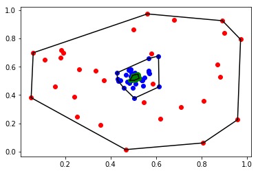
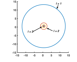
Below in Figure 1, we briefly illustrate the result in Thoerem III.2 via an example, for the update with being row stochastic a 30 node Erdos-Rényi graph is initialized with values chosen uniformly at random from . The initial values are displayed in red, with the boundary of the convex hull traced in black. The points of are displayed in red, in blue, in green, with the convex hull boundaries of the respective sets traced in black. That row stochastic updating is convex decreasing is instantiated in the nested-ness of the sets .
When , the convex hull is simply described, , so that gives the monotonicity results from [26], and . Analogously, applying Theorem III.2 in the one dimensional case delivers the monotonicity of min and max from [23]. In the -dimensional case, taking to be the family of all rectangular sets recovers Theorem of [13].
We will use the monotonicity of convex decreasing consensus algorithms to develop a distributed stopping criteria, guaranteeing convergence of all nodes within an -ball of the consensus value for a general norm. First we develop a distributed convex hull computation algorithm that is of independent interest. Here, given a function the convex hull is to be determined by the network in a distributed fashion. Consider a algorithm where at stage one, agents share their value with neighbors. The nodes then update their approximation of the convex hull, by determining the extreme points among all values received from their neighbors and their own. This new set of extreme points is communicated to all neighbors and then the process repeats. We show that after ( being the diameter of the network) iterations, every node will have determined the extreme points of .
In the context of a consensus algorithm protocol represents or the value at node in iteration of a consensus algorithm, and we implement the following stopping criterion. Given a norm and a tolerance , implement the convex hull algorithm at time , then at time , at a node if , then stop the consensus algorithm. In what follows we demonstrate that upon stopping every node is within of the consensus value in norm.
IV Peer to Peer Convex Hull Algorithm
We now describe a finite time algorithm for distributed convex hull computation. Suppose that agents indexed by where each agent has a set of elements of . The agent can communicate with each other while respecting constraints imposed by a specific communication network. We provide a distributed consensus algorithm through which all agents obtain in -iterations of the algorithm. If we let denote the space of all finite sequences of elements of , the convex hull algorithm can be understood as a distributed consensus algorithm.
Definition 22.
For , define the initialization . Iteratively define,
We identify with an element of , by writing its elements in lexicographical order.
That is, at iteration , an agent receives the extreme points known to their “in-neighbors” and forms a new set comprised of their previous extreme points and their neighbors. Agent finds the extreme points of this new set, and then communicates the set to its “out-neighbors” to initiate another iteration.
Theorem IV.1.
Proof.
The result is true by definition checking when , since . Thus we proceed by induction and assume the result holds for . By definition,
| (12) |
By the induction hypothesis,
Recall that for non-convex sets , , so that
where the subscript ranges over the set . If we write , and apply Lemma II.1, with the fact that is convex and compact,
By definition of and another application of Lemma II.1,
Thus our result follows once we can show,
Both sets can be considered as unions of indexed by paths of length not larger than terminating at . More explicitly, both sets can be written as where is the space of all paths such that , . This gives (11). Since for , and . Thus the algorithm considers is a consensus algorithm. The algorithm is distributed as each is a function of the for . ∎
This shows that, agents in a distributed network can obtain exact knowledge of the convex hull in iterations. As an application the convex hull algorithm can be used to provide finite time stopping criterion for a convex decreasing consensus algorithm. We need the following lemma.
Lemma IV.1.
For a norm and a convex set ,
Proof.
For fixed that, is convex and hence takes its maximum value on at extreme value of . Hence , applying the same argument again we obtain
and our result follows. ∎
Theorem IV.2.
If denotes the vector at node at time in a convex-decreasing consensus algorithm, then for
Proof.
Denoting by the element of defined by , the assumption that is convex decreasing implies for , and hence for all . Thus, as well and we have
∎
It follows that an agent can obtain exact bounds on the distance from convergence of the consensus with respect to an arbitrary norm.
Standard algorithms for computing the convex hull of a set of points in -dimensional exist, see [43, 44]. However such can easily be prohibitively expensive especially in high dimension (worst case runtime is of the order ), when computational resources, or communication power is limited. Further, in the worst case scenario, the number of extreme points can be of the same order as the nodes of the graph (take to be points of a -dimensional sphere for instance), and hence their communication cost is equivalent to that of the entire system state. In the following section we develop a stopping algorithm to address these potential feasibility issues.
V Norm Based Finite-Time Termination
Similar to the convex hull comprising all points (corresponding to each agent), radius of a minimal ball in dimension enclosing all the points can also be used as a termination criterion. Once the radius is within some bound , it can be shown that every agent’s state is within of the consensus value. We remark that even in the case determination of a minimum norm ball in a distributed manner is a difficult problem (see [45]). Here, we provide an algorithm which distributedly finds an approximation of minimal ball at each agent. We next show that the minimal ball is enclosed in this approximation, thus if the approximate ball’s radius is within then the minimal ball’s radius is within as well. This is established in next Lemma.
Lemma V.1.
Let be the sequence generated by a distributed convex-decreasing consensus protocol. For all , let
| (13) | ||||
| (14) |
with and . Then
| (15) |
for all , where denotes the closed ball of radius centered at and is the diameter of the underlying graph topology.
Proof.
We first prove the following claim.
| (16) |
for all such that the length of the shortest path from to is less than equal to Clearly above claim is sufficient to prove (15) as when , (16) is valid for all . Let the length of the shortest path from to be denoted as . We prove the claim using induction. For ,
Then for all , that is for all such that , we get
Thus the assertion holds for . Now lets assume (16) is true for . Let be a node such that . Let be a neighbor of on the shortest path from to , then . Then from induction assumption,
that is,
| (17) |
From definition of ,
From triangle inequality,
Using (17),
which implies that
and thus,
and the result follows. ∎
Lemma V.1 provides a distributed way to find a ball which encloses all the nodes. Only information needed by a node is the current radius of its neighbors (along with the states pertaining to ratio consensus) and it can determine the final radius within iteration. Further, since the ball encloses all the nodes, it also encloses the minimum ball, as mentioned earlier. Thus we have provided an algorithm to find an approximation of the minimum ball comprising of all nodes. We next present a framework which we use to prove that this radius converges to and can be used as a distributed stopping criterion.
Consider the coordinate-wise maximum and minimum of the states taken over all the agents at atime instant be given by, and respectively. That is,
| (18) | ||||
| (19) |
where , for all and is the -th elements of . Then from [24], for all time instants and for all and ,
| (20) |
Further from [24], for all and ,
| (21) | ||||
| (22) |
By using (20), (21) and (22), we can prove the following theorem.
Theorem V.1.
Proof.
It follows from Theorem III.1 that for all . This implies that for all , and given , there exists a such that for all . This implies that, there exists such that for all . Similarly, . Thus, it follows that, and . As subsequences of convergent subsequences, the same conclusion follows for and . ∎
Corollary V.1.
Proof.
The proof directly results from Theorem V.1. ∎
It is clear from Lemma V.1 that at any instant , all agents’ states are within of each other, that is,
| (24) |
Thus if is within a tolerance , all the agents ratio state will be within of consensus. We next provide convergence result for as .
Theorem V.2.
For a distributed convex decreasing consensus algorithm and update as in (13). Let for and all Then
for all
Proof.
From definition,
which implies,
| (25) |
Let and be as defined in Theorem V.1. As and from (20), we get
| (26) |
Then using (26) in (25) and observing for all , we get
| (27) |
Similarly,
| (28) |
Again as and , we have
| (29) |
Then using (27), (28) and (29), we get
Following the same process, we have
| (30) |
Then from Corollary V.1,
∎
Notice that can be different for different nodes and each node might detect -convergence () at different time instants. According to Lemma V.1, once for any , , that is the ratio state is within of consensus value, and the consensus is achieved. Further, any node which detects convergence can propagate a “converged flag” in the network. To take that into account, we run a separate -bit consensus algorithm (denoted as convergence consensus) for each node where each node maintains a convergence state and shares it with neighbors. Each node initializes at every iteration for with or depending on the node has detected convergence or not, and updates its value on every iteration using,
| (31) |
where denotes OR operation, and if node has detected convergence at initialization instant and otherwise. Clearly, if for any , then for all where is the diameter. Thus each node can use as a stopping criterion.
Using above discussion and Theorem V.2, we present an algorithm (see Algorithm 1) instantiating the result for ratio consensus (which could easily be adapted for more general settings), which determines the radius for and all and provides a finite-time stopping criterion for vector consensus.
Theorem V.3.
Algorithm 1 converges in finite-time simultaneously at each node.
Proof.
From Corollary V.1, it follows that as Thus, for any given and node there exists an integer such that for . As each node has access to , convergence can be detected by each node and the convergence bit will be set to 1. Thus for all and algorithm will stop simultaneously at each node.∎
Remark 1.
Notice that using the above protocol, each node detects convergence simultaneously. Further, the only global parameter needed for Algorithm 1 is the knowledge of diameter . However, it should be noted that an upper bound will suffice. In most applications, an upper bound on the diameter is readily available.
Remark 2.
It is to note here that for Algorithm 1, only extra communication required between nodes is passing of the current radius at each node which is just a scalar along with a single bit for convergence consensus. Therefore the extra bandwidth required for each neighbor-neighbor interaction is where is the bit length (usually 32) for floating point representation. Thus, the above protocol is suitable for ad-hoc communication networks where communication cost is high and bandwidth is limited.
A finite-time termination criterion for vector consensus was previously provided in [13]. There, each element of ratio state required a maximum-minimum protocol (see (18) and (19)), with stopping criterion given by,
This maximum-minimum is a special case for finding a minimum convex set in the form of a hyper rectangle (box) which encompasses all the points. Here, at each iteration, two extra states are shared by each node, namely, one state for element-wise maximum and the other for element-wise minimum. Thus the extra communication bandwidth required for this algorithm is . An example case where , requires an extra bandwidth of bits per interaction. For this example, Algorithm 1 only requires extra bits of communication per interaction, providing a reduction of more than x. Thus for the applications with high dimensional vector consensus (like GANs, as described in the introduction, see [19]), the algorithm reported here provides a reliable distributed stopping criterion with significantly less communication bandwidth.
VI Applications of finite-time terminated average consensus in higher dimensions
VI-A Least Squares Estimation
We follow [46] in our exposition of the least squares problem as solved by consensus.
Consider the problem of estimating a function , given a noisy dataset under the assumption that is a linear combination of known functions . Explicitly . Defining for , vectors and to be the matrix formed by taking columns . Then taking for granted the invertibility of the relevant matrices, the least squares estimate of is given by taking
| (32) | ||||
| (33) | ||||
| (34) |
where the first equality is derived from setting the gradient of to zero and the second follows from algebra.
Initializing an average consensus algorithms on nodes, initialized to , a node , can form a consensus estimate of at time , by
| (35) |
Indeed, as an average consensus algorithm,
and
thus
For a matrix , let
Lemma VI.1.
[38] For invertible matrices, and ,
Theorem VI.1.
Note the terms and can be bounded through the finite time stopping criteria. Further the terms and depend only on locally computable terms. Thus the theorem demonstrates that not only can agents perform a distributed least square estimate, they can obtain error bounds on their estimates in a distributed fashion. That and ensure convergence of the algorithm.
VI-B Distributed Function Calculation
Here, we give another application of the average consensus protocol in higher dimensions. We focus on the problem of computing arbitrary functions of agent state values over sensor networks, see [34]. In particular, given a directed graph with nodes representing the communication constraints in a sensor network, the objective is to design an interaction rule for the nodes in the network to cooperatively compute a desired function , of the initial values . Such a problem is of interest in wireless sensor networks, see [34] where, the sink nodes in the sensor networks has to carry out the task of communicating a relevant function of the raw sensor measurements. Another example is the case of coordination tasks in multi-agent systems as given in [47], [11], where all agents communicate with each other to coordinate their speed and direction of motion. Consider, the directed graph modeling the interconnection topology between the agents. Let each agent maintain three variables denoted by and with the following initialization:
| (43) | ||||
| (44) | ||||
| (45) |
The estimates , and are updated according to (6), (7) and (9) respectively. The following theorem upper bounds the error in distributed function calculation by the error in the consensus estimation.
Theorem VI.2.
Let and associated with satisfy Assumptions 1 and 2 respectively. Denote by and the sequences generated by (6), (7) and (9) respectively. Under the initialization (43)-(45) the estimates asymptotically converges to for all , and is -Lipschitz, or more generally -Hölder continuous with constant , then
col
Proof.
The proof follows from Theorem II.2. In particular, by Theorem II.2 under Assumptions 1 and 2 the updates (9) converges to for all . With the initialization (43)-(45) the limiting value is given by
To complete the proof one only needs to apply the definition of -Hölder continuity, that , to the estimate and the consensus value . ∎
Remark 3.
Theorem VI.2 guarantees that for large enough values of the agents following update rules (6)-(9) will have enough information to calculate any arbitrary function of the initial values. Moreover, unlike the existing methods in the literature [35] which require carefully designed matrices based on the global information of the network the proposed scheme allows for distributed synthesis. Further, the finite-time terminated protocol discussed here is applicable for arbitrary time-invariant connected directed graphs unlike the stringent assumptions required for applicability of some schemes in the literature, see [48].
VII Results
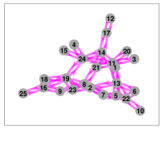
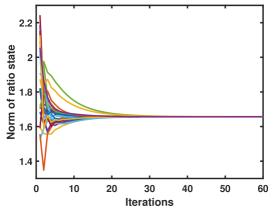
In this section, we present simulation results to demonstrate finite-time stopping criterion for high-dimensional ratio consensus. A network of 25 nodes is considered which is represented by a randomly generated directed graph (see Fig. 2(a)) with diameter . Here the numerator state is chosen to be a 10-dimensional vector and selected randomly for every node. Equation (6), (7) and (9) are implemented in MATLAB and simulated. 2-norm of each node’s ratio state is plotted in Figure 2(b) achieving convergence in iterations.
 |
 |
| (a) | (b) |
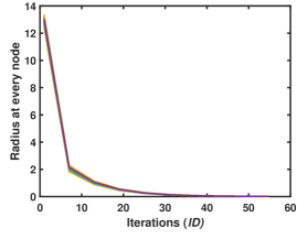
Algorithm 1 is implemented in MATLAB and the radius for all is plotted in Fig. 3(a). Here, it can be seen that radius comes under some pre-specified tolerance (, of the norm of the consensus vector) within 60 iteration and is used as a stopping criterion by each node. Fig. 3(b) plots the two dimensional projection of the ball for node as progresses over time. As expected, with increase in , balls shrink in size. Similar observation is seen for all the other nodes as well. The above illustration demonstrates how Algorithm 1 can be successfully used as finite-time termination criterion for distributed ratio consensus.
 |
 |
| (a) | (b) |
VIII Conclusion
In this article, we presented a notion of monotonicity of network states in vector consensus algorithms, which we called a convex decreasing consensus algorithm. We showed that this property can be used to construct finite-time stopping criterion and provided a distributed algorithm. We further provided an algorithm which calculates an approximation of minimum norm balls which contain all the network states at a given iteration. Radius of these balls was shown to converge to zero, and algorithm was presented to use that as a finite-time stopping criterion. This algorithm was shown to have much smaller communication requirement compared to existing methods. The effectiveness of our algorithm is validated by simulating a vector () ratio consensus algorithm for a network graph of 25 nodes. Further we demonstrated how these stopping criteria could be applied to provide guarantees on the convergence of Least Squared Estimator approximation through consensus.
References
- [1] K. J. Arrow and L. Hurwicz, Decentralization and computation in resource allocation. Stanford University, Department of Economics, 1958.
- [2] M. H. DeGroot, “Reaching a consensus,” Journal of the American Statistical Association, vol. 69, no. 345, pp. 118–121, 1974.
- [3] N. A. Lynch, Distributed algorithms. Elsevier, 1996.
- [4] J. N. Tsitsiklis, “Problems in decentralized decision making and computation.,” tech. rep., DTIC Document, 1984.
- [5] D. Kempe, A. Dobra, and J. Gehrke, “Gossip-based computation of aggregate information,” in 44th Annual IEEE Symposium on Foundations of Computer Science, 2003. Proceedings., pp. 482–491, IEEE, 2003.
- [6] A. D. Dominguez-Garcia and C. N. Hadjicostis, “Coordination and control of distributed energy resources for provision of ancillary services,” in Smart Grid Communications (SmartGridComm), 2010 First IEEE International Conference on, pp. 537–542, IEEE, 2010.
- [7] C. N. Hadjicostis and T. Charalambous, “Average consensus in the presence of delays in directed graph topologies,” IEEE Transactions on Automatic Control, vol. 59, no. 3, pp. 763–768, 2013.
- [8] K. Cai and H. Ishii, “Average consensus on general strongly connected digraphs,” Automatica, vol. 48, no. 11, pp. 2750–2761, 2012.
- [9] J. B. Predd, S. R. Kulkarni, and H. V. Poor, “A collaborative training algorithm for distributed learning,” IEEE Transactions on Information Theory, vol. 55, no. 4, pp. 1856–1871, 2009.
- [10] J. A. Fax and R. M. Murray, “Information flow and cooperative control of vehicle formations,” IFAC Proceedings Volumes, vol. 35, no. 1, pp. 115–120, 2002.
- [11] R. Olfati-Saber, J. A. Fax, and R. M. Murray, “Consensus and cooperation in networked multi-agent systems,” Proceedings of the IEEE, vol. 95, no. 1, pp. 215–233, 2007.
- [12] A. Nedić and A. Olshevsky, “Distributed optimization over time-varying directed graphs,” IEEE Transactions on Automatic Control, vol. 60, no. 3, pp. 601–615, 2014.
- [13] V. Khatana, G. Saraswat, S. Patel, and M. V. Salapaka, “Gradient-consensus method for distributed optimization in directed multi-agent networks,” arXiv preprint arXiv:1909.10070, 2019.
- [14] U. A. Khan, S. Kar, and J. M. Moura, “Distributed sensor localization in random environments using minimal number of anchor nodes,” IEEE Transactions on Signal Processing, vol. 57, no. 5, pp. 2000–2016, 2009.
- [15] U. A. Khan, S. Kar, and J. M. Moura, “Higher dimensional consensus: Learning in large-scale networks,” IEEE Transactions on Signal Processing, vol. 58, no. 5, pp. 2836–2849, 2010.
- [16] S. Patel, S. Attree, S. Talukdar, M. Prakash, and M. V. Salapaka, “Distributed apportioning in a power network for providing demand response services,” in 2017 IEEE International Conference on Smart Grid Communications (SmartGridComm), pp. 38–44, IEEE, 2017.
- [17] A. Nedic, A. Ozdaglar, and P. A. Parrilo, “Constrained consensus and optimization in multi-agent networks,” IEEE Transactions on Automatic Control, vol. 55, no. 4, pp. 922–938, 2010.
- [18] S. Chakraborty, A. Preece, M. Alzantot, T. Xing, D. Braines, and M. Srivastava, “Deep learning for situational understanding,” in 2017 20th International Conference on Information Fusion (Fusion), pp. 1–8, IEEE, 2017.
- [19] I. Goodfellow, J. Pouget-Abadie, M. Mirza, B. Xu, D. Warde-Farley, S. Ozair, A. Courville, and Y. Bengio, “Generative adversarial nets,” in Advances in neural information processing systems, pp. 2672–2680, 2014.
- [20] A. Kurakin, I. Goodfellow, and S. Bengio, “Adversarial machine learning at scale,” ICLR, 2017.
- [21] Z. Li, F. R. Yu, and M. Huang, “A distributed consensus-based cooperative spectrum-sensing scheme in cognitive radios,” IEEE Transactions on Vehicular Technology, vol. 59, no. 1, pp. 383–393, 2009.
- [22] S. Patel, V. Khatana, G. Saraswat, and M. V. Salapaka, “Distributed detection of malicious attacks on consensus algorithms with applications in power networks,” 2020.
- [23] V. Yadav and M. V. Salapaka, “Distributed protocol for determining when averaging consensus is reached,” in 45th Annual Allerton Conf, pp. 715–720, 2007.
- [24] M. Prakash, S. Talukdar, S. Attree, S. Patel, and M. V. Salapaka, “Distributed Stopping Criterion for Ratio Consensus,” in 2018 56th Annual Allerton Conference on Communication, Control, and Computing (Allerton), pp. 131–135, Oct. 2018.
- [25] G. Saraswat, V. Khatana, S. Patel, and M. V. Salapaka, “Distributed finite-time termination for consensus algorithm in switching topologies,” arXiv preprint arXiv:1909.00059, 2019.
- [26] M. Prakash, S. Talukdar, S. Attree, V. Yadav, and M. V. Salapaka, “Distributed stopping criterion for consensus in the presence of delays,” IEEE Transactions on Control of Network Systems, 2019.
- [27] S. Sundaram and C. N. Hadjicostis, “Finite-time distributed consensus in graphs with time-invariant topologies,” in 2007 American Control Conference, pp. 711–716, IEEE, 2007.
- [28] F. P. Preparata, “An optimal real-time algorithm for planar convex hulls,” Communications of the ACM, vol. 22, no. 7, pp. 402–405, 1979.
- [29] D. Fernández-Francos, Ó. Fontenla-Romero, and A. Alonso-Betanzos, “One-class convex hull-based algorithm for classification in distributed environments,” IEEE Transactions on Systems, Man, and Cybernetics: Systems, 2017.
- [30] P. Casale, O. Pujol, and P. Radeva, “Approximate polytope ensemble for one-class classification,” Pattern Recognition, vol. 47, no. 2, pp. 854–864, 2014.
- [31] L. Kavan, I. Kolingerova, and J. Zara, “Fast approximation of convex hull.,” ACST, vol. 6, pp. 101–104, 2006.
- [32] E. Osuna and O. De Castro, “Convex hull in feature space for support vector machines,” in Ibero-American Conference on Artificial Intelligence, pp. 411–419, Springer, 2002.
- [33] W. Kim, M. S. Stanković, K. H. Johansson, and H. J. Kim, “A distributed support vector machine learning over wireless sensor networks,” IEEE transactions on cybernetics, vol. 45, no. 11, pp. 2599–2611, 2015.
- [34] A. Giridhar and P. R. Kumar, “Computing and communicating functions over sensor networks,” IEEE Journal on selected areas in communications, vol. 23, no. 4, pp. 755–764, 2005.
- [35] S. Sundaram and C. N. Hadjicostis, “Distributed function calculation and consensus using linear iterative strategies,” IEEE journal on selected areas in communications, vol. 26, no. 4, pp. 650–660, 2008.
- [36] J. Melbourne, G. Saraswat, V. Khatana, S. Patel, and M. V. Salapaka, “On the geometry of consensus algorithms with application to distributed termination in higher dimension,” the proceedings of International Federation of Automatic Control (IFAC), 2020.
- [37] R. Diestel, Graph Theory. Berlin, Germany: Springer-Verlag, 2006.
- [38] R. A. Horn and C. R. Johnson, Matrix analysis. Cambridge university press, 2012.
- [39] R. T. Rockafellar, Convex analysis. No. 28, Princeton university press, 1970.
- [40] P. Lax, Functional Analysis, vol. 1. Wiley-Interscience, 2002.
- [41] D. A. Levin and Y. Peres, Markov chains and mixing times, vol. 107. American Mathematical Soc., 2017.
- [42] R. M. Gray and R. Gray, Probability, random processes, and ergodic properties, vol. 1. Springer, 2009.
- [43] K. L. Clarkson and P. W. Shor, “Applications of random sampling in computational geometry, ii,” Discrete & Computational Geometry, vol. 4, no. 5, pp. 387–421, 1989.
- [44] C. B. Barber, D. P. Dobkin, D. P. Dobkin, and H. Huhdanpaa, “The quickhull algorithm for convex hulls,” ACM Transactions on Mathematical Software (TOMS), vol. 22, no. 4, pp. 469–483, 1996.
- [45] K. Fischer, Smallest enclosing balls of balls. PhD thesis, ETH Zürich, 1975.
- [46] F. Garin and L. Schenato, “A survey on distributed estimation and control applications using linear consensus algorithms,” in Networked control systems, pp. 75–107, Springer, 2010.
- [47] W. Ren, R. W. Beard, and E. M. Atkins, “A survey of consensus problems in multi-agent coordination,” in Proceedings of the 2005, American Control Conference, 2005., pp. 1859–1864, IEEE, 2005.
- [48] D. B. Kingston and R. W. Beard, “Discrete-time average-consensus under switching network topologies,” in 2006 American Control Conference, pp. 6–pp, IEEE, 2006.
![[Uncaptioned image]](https://cdn.awesomepapers.org/papers/92d9ef72-d28f-482d-afdd-2a4fc3433213/James.jpg)
|
James Melbourne received his Bachelors in Art History in 2006 and a Masters in Mathematics in 2009 both from the University of Kansas, and his PhD in Mathematics in 2015 at the University of Minnesota. He was a postdoctoral researcher in the University of Delaware Mathematics department from 2015 to 2017, and is currently a postdoctoral researcher at the University of Minnesota in Electrical and Computer Engineering. His research interest include convexity theory, particularly its application to probabilistic, geometric, and information theoretic inequalities, consensus algorithms, and stochastic energetics. |
![[Uncaptioned image]](https://cdn.awesomepapers.org/papers/92d9ef72-d28f-482d-afdd-2a4fc3433213/Saraswat_Govind.jpg)
|
Govind Saraswat received his B.Tech degree in Electrical Engineering from the Indian Institute of Technology, Delhi, in 2007 and his PhD degree in Electrical Engineering from University of Minnesota, Twin Cities in 2014. Currently, he is part of Sensing and Predictive Analytics group at National Renewable Energy Laboratory, Golden, CO (NREL) where he works on data-driven technology for energy systems planning and operation. His research includes power system modeling and analysis, measurement-based operation and control, machine learning, and optimization. |
![[Uncaptioned image]](https://cdn.awesomepapers.org/papers/92d9ef72-d28f-482d-afdd-2a4fc3433213/Vivek.jpg)
|
Vivek Khatana received the B.Tech degree in Electrical Engineering from the Indian Institute of Technology, Roorkee, in 2018. Currently, he is working towards a Ph.D. degree at the department of Electrical Engineering at University of Minnesota. His Ph.D. research interest includes distributed optimization, consensus algorithms, distributed control and stochastic calculus. |
![[Uncaptioned image]](https://cdn.awesomepapers.org/papers/92d9ef72-d28f-482d-afdd-2a4fc3433213/x5.jpg)
|
Sourav Kumar Patel received his B.Tech. degree in Instrumentation and Control Engineering from the National Institute of Technology, Jalandhar, in 2011. In the same year, he joined National Thermal Power Corporation Ltd. in Kaniha, Odisha, India as a Control and Instrumentation Engineer. He received his M.S. degree in Electrical Engineering from the University of Minnesota, Twin-Cities, in 2018 where currently, he is working towards his Ph.D. degree in Electrical Engineering. His research interests include control and systems theory, coordination and communication protocols for Distributed Energy Resources towards smart grid applications. |
![[Uncaptioned image]](https://cdn.awesomepapers.org/papers/92d9ef72-d28f-482d-afdd-2a4fc3433213/salapaka.jpg)
|
Murti V. Salapaka received the B.Tech. degree in Mechanical Engineering from the Indian Institute of Technology, Madras, in 1991 and the M.S. and Ph.D. degrees in Mechanical Engineering from the University of California at Santa Barbara, in 1993 and 1997, respectively. He was a faculty member in the Electrical and Computer Engineering Department, Iowa State University, Ames, from 1997 to 2007. Currently, he is the Director of Graduate Studies and the Vincentine Hermes Luh Chair Professor in the Electrical and Computer Engineering Department, University of Minnesota, Minneapolis. His research interests include control and network science, nanoscience and single molecule physics. Dr. Salapaka received the 1997 National Science Foundation CAREER Award and is an IEEE fellow. |