Cooperative Beam Hopping for Accurate Positioning in Ultra-Dense LEO Satellite Networks
Abstract
In ultra-dense LEO satellite networks, conventional communication-oriented beam pattern design cannot provide multiple favorable signals from different satellites simultaneously, and thus leads to poor positioning performance. To tackle this issue, in this paper, we propose a novel cooperative beam hopping (BH) framework to adaptively tune beam layouts suitable for multi-satellite coordinated positioning. On this basis, a joint user association, BH design and power allocation optimization problem is formulated to minimize average Cramér-Rao lower bound (CRLB). An efficient flexible BH control algorithm (FBHCA) is then proposed to solve the problem. Finally, a thorough experimental platform is built following the Third Generation Partnership Project (3GPP) defined non-terrestrial network (NTN) simulation parameters to validate the performance gain of the devised algorithm. The numerical results demonstrate that FBHCA can significantly improve CRLB performance over the benchmark scheme.
Index Terms:
Multibeam LEO satellite, TDOA positioning, beam hopping, Cramér-Rao lower bound, 3GPP NTN.I Introduction
With the advent of New Space era, satellite communication has gained a renewed upsurge due to its ability to provide global wireless coverage and continuous service guarantee especially in scenarios not optimally supported by terrestrial infrastructures[1, 2]. Specifically, some standardization endeavors have been sponsored by the Third Generation Partnership Project (3GPP) to study a set of necessary adaptations enabling the operation of 5G New Radio (NR) protocol in non-terrestrial network (NTN) with a priority on satellite access [3, 4]. In the NTN context, compared with conventional geostationary earth orbit (GEO) and medium earth orbit (MEO), low earth orbit (LEO) based satellite networks stand out as a promising solution concerning the lower propagation delay, power consumption and launch cost. As such, numerous companies have announced ambitious plans to provide broadband Internet access over the globe by deploying LEO satellite mega-constellations, e.g., Oneweb, Kuiper and Starlink.
On the other hand, the rapid proliferation of location-based services, e.g., smart transportation, augmented reality and autonomous driving, bring marvellous value-added opportunities to communication networks. Besides, location-aided communication optimization such as enhanced access control and simplified mobility management can be fully exploited to improve network scalability, latency, and robustness [5]. Given those benefits, it is imperative to provide high precision positioning information on top of communication networks. As stipulated by NR Release-16, a positioning accuracy of 3-meter within 1 second end to end latency should be achieved for commercial use cases, and subsequent releases are expected to further realize sub-meter localization accuracy and millisecond level lower latency [6]. This induces great challenge to meet such stringent requirements.
To circumvent this issue, a plenty of research efforts on localization techniques have been conducted from both the academic and industry communities [7, 8]. In terrestrial cellular networks, numerous ranging measurement based positioning schemes, e.g., time of arrival (TOA), time difference of arrival (TDOA), angle of arrival (AOA), and received signal strength (RSS), are devised to figure out source location. Nevertheless, those positioning schemes cannot be directly applied to LEO satellite communication, owing to its unique characteristics such as dynamic network topology, strong multibeam interference, and channel model. While in the satellite scenario, state of the art positioning studies mainly focus on range error analysis, e.g., Cramér-Rao lower bound (CRLB), from a macroscopic constellation design perspective [9, 10]. However, the concrete multibeam structure design philosophy and underlying beam management problem to optimize positioning performance remain unexplored in LEO mega-constellation communication networks.
It is technically challenging to develop accurate positioning schemes for ultra-dense LEO satellite networks, due to several reasons: 1) A LEO satellite generally suffers from limited available onboard payload, and thus only a few physical transceivers/beams can be utilized. These beams should be efficiently shared for dual functional communication and positioning purposes. However, conventional communication oriented multibeam design cannot guarantee multiple strong signals from different satellites, and thus significantly degrades localization performance; 2) Since there is no near-far effect, the interference problem in satellite environment becomes critical. Besides, the fast mobility of LEO satellites makes the multibeam interference more complex and time-varying [11]; 3) To support accurate localization, it is essential to perform coordinate beam management among multiple satellites. The problem is quite difficult to handle considering both the nonlinearity of optimization metric and intrinsic coupling within user association, power/beam allocation and interference.
In this paper, to address the aforementioned challenges, we investigate the positioning oriented multibeam pattern design as well as the beam management problem in LEO mega-constellation communication system. The main contributions of this paper are summarized as follows. Firstly, we propose a novel cooperative beam hopping (BH) framework to flexibly tune the physical beam layout for optimized positioning usage. On the basis, an average CRLB minimization problem subject to user association, BH management and power allocation related constraints is formulated. Secondly, a flexible BH control algorithm (FBHCA) is proposed to decompose the original problem into three sub-problems, i.e., user association, BH design and power allocation sub-problems, which are further solved by max-SINR criteria, Voronoi diagram and semi-definite programming (SDP) technique, respectively. Finally, we provide extensive simulations in calibrated 3GPP NTN platform to evaluate the effectiveness of FBHCA and demonstrate its CRLB performance gain over existing schemes.
The remainder of this paper is organized as follows. Section II introduces the system model and presents the cooperative BH framework. The optimization problem formulation and corresponding FBHCA solution are investigated in Section III and Section IV, respectively. Section V provides the simulation results, followed by conclusions in Section VI.
II System Model and BH Framework
II-A System Model
We consider an orthogonal frequency division multiplexing (OFDM) based ultra-dense LEO multibeam satellite network. The satellite system operates at a center frequency with total system bandwidth . To mitigate intra-satellite inter-beam interference, a frequency/polarization reuse factor of is applied. For inter-satellite interference reduction, time/frequency/code domain multiplexing can be utilized, and such kind of interference is neglected. For example, the positioning reference signal design with frequency reuse and muting configuration in 3GPP LTE can mitigate inter-cell interference. In the network, there are a set of LEO satellites. A satellite is equipped with a set of beams. For beam allocation, we further define a binary variable if beam is allocated by satellite , and otherwise. A set of user equipments (UEs) are distributed requesting for positioning service. For a user , the associated set of satellites used for positioning is denoted as . The TDOA positioning scheme is adopted to calculate UE location results.
As per 3GPP NTN specifications [4], the following satellite antenna pattern is considered
| (1) |
where is the Bessel function of the first kind and first order with the argument, is the antenna aperture radius, is the steering angle, and is the light propagation speed. Meanwhile, the total path loss consists of following components:
| (2) |
where is the shadow fading modeled by a log-normal distribution , is the slant path distance, and and represent the atmospheric absorption and scintillation loss, respectively. The power received by the -th user from -th beam of -th satellite is
| (3) |
where and denote the angle and distance between user and beam in satellite , respectively. Besides, is the transmitted Equivalent Isotropically Radiated Power density allocated to beam in satellite , is the beam transmit power, and and denote the constant transmit and receive antenna gain, respectively. To this end, the overall signal-to-interference plus noise ratio (SINR) is
| (4) |
where is the noise power determined by UE noise figure and antenna temperature [4].
II-B Cooperative Beam Hopping Design
As a promising solution, BH is devised to employ only a small subset of transceivers/beams for serving extensive satellite coverage area. More specifically, assuming that a satellite aims to achieve a coverage of beams by using beams with . For this purpose, at each time stamp, a maximum number of beams are assigned to illuminate a portion of the whole satellite coverage area, and time-division multiplexing approach is implemented to manipulate the set of beams into different portions within the coverage area of beams. Through flexible beam allocation, full satellite coverage can be eventually served.
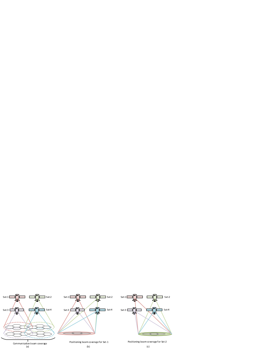
To support accurate positioning, we exploit BH to adaptively tune the physical beam layout from communication-oriented to positioning-oriented design. With cooperative BH from multiple neighboring satellites, localization performance can be significantly improved for UEs in a target satellite. An example BH for dual functional communication and positioning beams in a 4-satellite scenario is depicted in Fig. 1. On the one hand, communication beams are generally pointed to coverage area centered at the satellite nadir as in Fig. 1(a), such that seamless coverage is formed. On the other hand, to enhance localization performance, a set of neighbor satellites need to direct their beams to the target satellite. The center point of positioning beams normally stays far away from satellite nadir point. The cooperative BH patterns for positioning of Sat-1 and Sat-2 are sketched in Fig. 1(b) and Fig. 1(c), respectively.
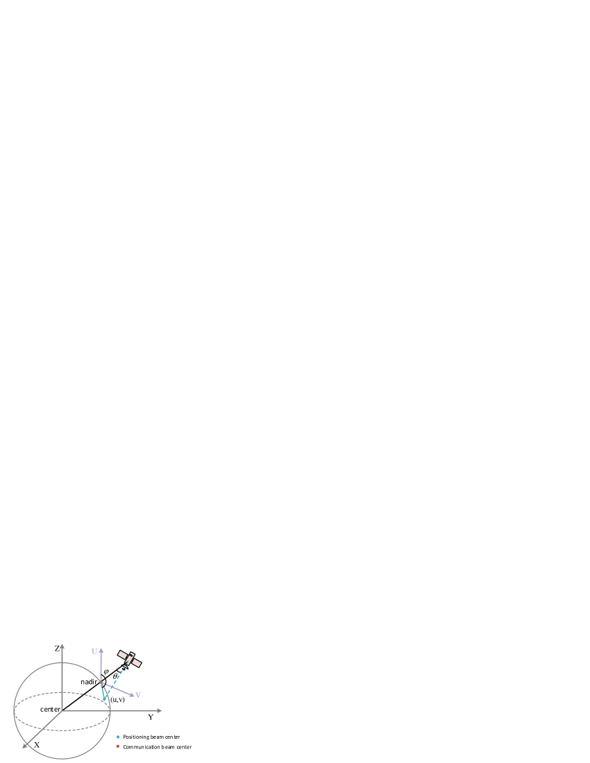
An efficient UV plane based BH scheme (UVBHS) is devised for beam operation. As plotted in Fig. 2, UV plane is defined as the perpendicular plane to the satellite-earth line on the orbital plane. In UVBHS, a hexagonal beam layout is defined on the UV plane with UV coordinate of the nadir of the reference satellite setting to (0,0) for communication beams. For positioning beams, there are two different configuration situations. Firstly, to perform localization in its own service area, the satellite can simply reuse the communication configurations for positioning usage. Secondly, to assist localization for a neighboring satellite, the satellite needs to translate the beams centered at (0,0) to the center of the neighbor satellite’s nadir in the UV plane denoted by . We can derive and , where and represent beam bore-sight steering angle and azimuth, respectively.
III Optimization Problem Formulation
III-A CRLB Analysis
In the mean squared error (MSE) sense, CRLB gives the lowest possible variance that an unbiased linear estimator can achieve. To this end, we use CRLB as the accuracy indicator for TDOA positioning error analysis.
III-A1 TOA Measurement in OFDM system
For TDOA positioning, a set of TOA measurements from multiple satellites should be conducted at first. In an OFDM system, denote as the signal allocated on the -th subcarrier of the -th symbol. The number of symbols and subcarriers used for positioning is expressed as and , respectively. According to [12], under a static AWGN channel, the MSE of TOA measurement at satellite is calculated by
| (5) |
where is the OFDM symbol duration, denotes the association variable of user to beam in satellite , and .
III-A2 CRLB analysis for TDOA positioning
Based on the above TOA measurements, the CRLB for TDOA positioning at a target UE is explicitly analyzed herein. The positions of UE and satellites are denoted as and , respectively. The distance between the target UE and satellite is expressed as
| (6) |
Without loss of generality, we choose as the reference satellite location. Under a line of sight (LOS) scenario prevalent in satellite context, the TDOA received by and is
| (7) |
where is the TOA measurement noise with zero mean and covariance . The CRLB for estimating in user equals
| (8) |
where , is the trace operator of matrix, and
III-B Average CRLB Minimization Problem Optimization
Based on the envisioned cooperative BH framework, i.e., UVBHS, an average CRLB optimization problem is formulated to improve positioning accuracy.
| (9) |
In problem (9), the objective is to minimize average CRLB of UEs by optimizing decision variables , , and . Constraints C1 states that each user should be associated to at most one beam at a given satellite; C2 specifies that the beam should be allocated once a user is associated to the beam, where is a sufficiently large integer; C3 is the individual beam power constraint; and C4 is imposed to guarantee that the allocated power at a satellite should not exceed its total available power. The NP-hardness of the optimization problem is shown below.
Lemma 1.
Problem (9) is NP-hard.
IV Proposed Solution
Herein, the problem is first decomposed and an efficient FBHCA solution is proposed, followed by complexity analysis.
IV-A Problem Decomposition based Solution
The problem (9) is solved by decomposing it into three sub-problems, namely, user association sub-problem, BH design sub-problem, and power allocation sub-problem.
IV-A1 User association
To solve the user association sub-problem, the following lemma is introduced.
Lemma 2.
The is a monotonically decreasing function of .
Proof:
Define and , where are column vectors with a length of . Besides, . According to the Matrix Inversion Lemma, we obtain
where . On the basis, the CRLB expression can be equivalently written as follows
| (14) | |||
where , and . Consider that holds for a typical LEO satellite network, and thus the value of dominates the final result. Consequently, decreases as increases. ∎
According to Lemma 2, if the initial power allocation is given, the SINR can be computed using (4). Therefore, is optimally solved by attaching user to the beam with maximum SINR for satellite , which is
| (15) |
Note that for positioning purpose, association to multiple satellites is required for a UE. This is different from user attachment to only one serving satellite in communication oriented design. Given maximum SINR based user association criteria, the decisions of are easily obtained.
IV-A2 BH design
After solving , problem (9) can be further reformulated as
| (18) |
where the objective is rewritten by using (14), and the auxiliary variable satisfies
| (19) |
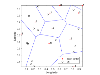
Meanwhile, the constraint C7 in reformulated problem (18) is added based on the Schur complement law [13]. Since the only non-convex decision variables in problem (18) are , an efficient Voronoi diagram [14] is used to solve the beam allocation problem. More specifically, each beam corresponds to a polygon representing its serving coverage area. We set if at least one user lies in the Voronoi area, and otherwise. To this end, the BH design sub-problem is successfully tackled. An example Voronoi graph for a 10-beam satellite is given in Fig. 3, where a polygon formed by several blue lines corresponds to a beam serving area. Note that because no UE attaches to beam 4 in Fig. 3, can be determined for the satellite.
IV-A3 Power allocation
Until now, the original problem is reduced to a power allocation problem with convex constraints
| (20) |
The above sub-problem (20) is a typical SDP problem, and can be efficiently solved by existing convex optimization methods, e.g., the interior-point method [15]. The obtained power results are capitalized to update the preceding power vector. Then, the algorithm moves forward to the next iteration. The iterations cease until a predetermined number is reached. The detailed procedure of FBHCA is summarized in Algorithm 1.
IV-B Complexity Analysis
The computational complexity of the devised algorithm is discussed herein. Recall that there are users, beams per satellite, and satellites used for positioning. The complexity of FBHCA comprises three parts: 1) User association with the complexity of . The complexity comes from a total of SINR calculations and comparisons for all UEs; 2) BH design with the complexity of . This is because for a points Voronoi diagram, the complexity is [16]. Besides, the Voronoi graph is generated for satellites, and calculations are required to decide the beam allocation variable . This results in a total complexity of ; 3) Power allocation with the complexity of . For each satellite, solving the SDP problem incurs worst-case complexity, and a set of satellites needs to be calculated for power allocation.
The algorithm runs iteratively to obtain the desired solution. There are iterations in total, with each iteration generating a complexity of . Overall, the computational complexity of FBHCA is derived as .
V Performance Evaluation
In this section, simulation settings following 3GPP NTN assumptions are first configured. Afterwards, numerical results are presented to verify the effectiveness of the algorithm.
V-A Simulation Settings
The set of key parameters used for simulations are summarized in Table I. Particularly, the satellite network comprises a total of 2400 satellites, with an orbit height varying from 800 km to 1500 km and inclination of 87.5 degree. The synchronization signal blocks (SSBs) in 3GPP NR are used for ToA measurements. The value of for shadow fading is a function of elevation angle following Table 6.6.2-3 in [4]. For dynamic simulation, the orbit period is divided into 100 snapshots of equal time duration. A total of 500 stationary UEs are randomly deployed in the target area with longitude and latitude setting to [-70,-60] and [-5,5], respectively. Note that all simulations are performed by extending the already calibrated platform for 3GPP NTN [17].
| Parameters | Values |
|---|---|
| The number of orbit | 40 |
| The number of satellite per orbit | 60 |
| Orbit inclination | 87.5 |
| Orbit height | [800,1500] km |
| The number of beam per satellite | 61 |
| Carrier frequency | 2 GHz |
| Satellite transmit antenna gain | 30 dBi |
| Maximum beam transmit power | 110 W |
| Total satellite power | 6100 W |
| System bandwidth | 30 MHz |
| Frequency reuse factor | 3 |
| Equivalent satellite antenna aperture | 0.5 m |
| Channel model | Clear sky with LOS |
| Atmospheric absorption loss | 0.1 dB |
| Scintillation loss | 2.2 dB |
| UE noise figure | 7 dB |
| Antenna temperature | 290 K |
| Subcarrier spacing | 15 KHz |
| Number of satellites for positioning | 4, 6, 8 |
V-B Numerical Results
| Algorithms | SNR for different satellites | |||
|---|---|---|---|---|
| Satellite 1 | Satellite 2 | Satellite 3 | Satellite 4 | |
| TMCB | 14.2 | -6.4 | -12.0 | -10.9 |
| UVBHS+EPA | 14.2 | 10.2 | 9.8 | 13.9 |
| FBHCA | 14.6 | 10.7 | 10.4 | 14.0 |
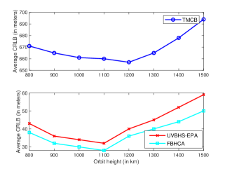
For comparison, two benchmark algorithms are used. One is the traditional method using communication beams (TMCB) for multi-satellite positioning as shown in Fig. 1(a). In TMCB, maximum SINR based user association and equal power allocation among all satellite beams are assumed. The other one is termed as UVBHS-EPA, which combines the proposed UVBHS framework with equal power allocation.
Fig. 4 depicts the average CRLB performance for different schemes as orbital height changes. As orbit height increases, the CRLB of all the three algorithms first decreases. The reason is that the constellation of 2400 satellites is not sufficient to provide full coverage for lower orbit height than around 1100 km. Lower orbit can cause worse SINR and positioning performance. With orbit height further rising, the CRLB increases as well due to the larger experienced path loss. Besides, both UVBHS-EPA and FBHCA significantly outperform TMCB in terms of CRLB. This is because in TMCB, although the received signal quality from the serving satellite is favorable, the signal quality from neighboring satellites is very poor due to the long distance between UE and beam center. Nonetheless, in the other two methods, neighboring satellite beams are directed to cover UEs of interest, and thus multiple signals with good quality can be measured to enhance positioning accuracy. To verify the performance gain, we list the SNR values of different satellites in Table II.
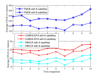
The CRLB results for different schemes as time snapshot varies are given in Fig 5. The orbit height is fixed to 1200 km in the simulation. All the algorithms exhibit CRLB fluctuation as time snapshots change. The variation tendency is quite complicated, due to the intertwined influence by time varying inter-beam interference and dynamic geometric dilution of precision. Besides, as the number of positioning satellites increases from 6 to 8, the CRLBs for all the three algorithms improve as well. This phenomena can be expected, because more signals and better network geometry are obtained by exploring satellite diversity.
VI Conclusion
In this paper, we have investigated the problem of high accuracy positioning in ultra-dense LEO satellite networks. A BH framework is proposed for flexible beam operation. With the framework, we further devise an efficient FBHCA solution to handle the joint user association, BH design, and power allocation problem. Significant positioning performance improvement in terms of average CRLB is demonstrated through 3GPP NTN simulation platform. As for future work, we tend to take inter-satellite interference issue into account and deal with the positioning reference signal design problem to further enhance localization accuracy.
References
- [1] M. Sheng, Y. Wang, J. Li, R. Liu, D. Zhou, and L. He, “Toward a flexible and reconfigurable broadband satellite network: resource management architecture and strategies,” IEEE Wireless Commu., vol. 24, no. 4, pp. 127–133, 2017.
- [2] O. Kodheli and et al., “Satellite communications in the new space era: A survey and future challenges,” arXiv preprint arXiv:2002.08811, pp. 1–45, Mar. 2020.
- [3] 3GPP TR 38.821 V16.0.0, “Solutions for NR to support non-terrestrial networks (NTN),” Release 16, Dec. 2019.
- [4] 3GPP TR 38.811 V15.0.0, “Study on new radio (NR) to support non terrestrial networks,” Release 15, Jun. 2018.
- [5] R. Taranto and et al., “Location-aware communications for 5G networks: How location information can improve scalability, latency, and robustness of 5G,” IEEE Signal Process. Mag., vol. 31, no. 6, pp. 102–112, Nov. 2014.
- [6] 3GPP TR 38.855 V16.0.0, “Study on new radio (NR) positioning support,” Release 16, Mar. 2019.
- [7] C. Laoudias and et al., “A survey of enabling technologies for network localization, tracking, and navigation,” IEEE Commun. Surveys Tuts., vol. 20, no. 4, pp. 3607–3644, 2018.
- [8] J. Peral-Rosado and et al., “Survey of cellular mobile radio localization methods: From 1G to 5G,” IEEE Commun. Surveys Tuts., vol. 20, no. 2, pp. 1124–1148, 2nd Quart., 2018.
- [9] T. Reid, A. Neish, T. Walter, and P. Enge, “Broadband LEO constellations for navigation,” NAVIGATION, Journal of the Institute of Navigation, vol. 65, no. 2, pp. 205–220, 2018.
- [10] F. Shu, S. Yang, Y. Qin, and J. Li, “Approximate analytic quadratic-optimization solution for TDOA-based passive multi-satellite localization with earth constraint,” IEEE Access, vol. 4, pp. 9283–9292, 2016.
- [11] Y. Wang, M. Sheng, W. Zhuang, S. Zhang, N. Zhang, R. Liu, and J. Li, “Multi-resource coordinate scheduling for earth observation in space information networks,” IEEE J. Sel. Areas Commun., vol. 36, no. 2, pp. 268–279, 2018.
- [12] J. Peral-Rosado and et al., “Achievable localization accuracy of the positioning reference signal of 3GPP LTE,” in Int. Conf. on Localization and GNSS, Jun. 2012, pp. 1–6.
- [13] S. Joshi and S. Boyd, “Sensor selection via convex optimization,” IEEE Trans. Signal Process., vol. 57, no. 2, pp. 451–462, Feb. 2009.
- [14] N. Okati, T. Riihonen, D. Korpi, I. Angervuori, and R. Wichman, “Downlink coverage and rate analysis of low earth orbit satellite constellations using stochastic geometry,” IEEE Trans. on Commun., vol. 68, no. 8, pp. 5120–5134, 2020.
- [15] S. Boyd and L. Vandenberghe, Convex Optimization. New York, NY, USA: Cambridge Univ. Press, 2004.
- [16] M. J. Golin and H.-S. Na, “On the average complexity of 3d-voronoi diagrams of random points on convex polytopes,” Computational Geometry, vol. 25, no. 3, pp. 197–231, 2003.
- [17] Huawei, HiSilicon, R1-1911858, “Discussion on performance evaluation for NTN,” RAN1#99, 2019.