Cooperative Learning-Based Framework
for VNF Caching and Placement Optimization
over Low Earth Orbit Satellite Networks
Abstract
Low Earth Orbit Satellite Networks (LSNs) are integral to supporting a broad range of modern applications, which are typically modeled as Service Function Chains (SFCs). Each SFC is composed of Virtual Network Functions (VNFs), where each VNF performs a specific task. In this work, we tackle two key challenges in deploying SFCs across an LSN. Firstly, we aim to optimize the long-term system performance by minimizing the average end-to-end SFC execution delay, given that each satellite comes with a pre-installed/cached subset of VNFs. To achieve optimal SFC placement, we formulate an offline Dynamic Programming (DP) equation. To overcome the challenges associated with DP, such as its complexity, the need for probability knowledge, and centralized decision-making, we put forth an online Multi-Agent Q-Learning (MAQL) solution. Our MAQL approach addresses convergence issues in the non-stationary LSN environment by enabling satellites to share learning parameters and update their Q-tables based on distinct rules for their selected actions. Secondly, to determine the optimal VNF subsets for satellite caching, we develop a Bayesian Optimization (BO)-based learning mechanism that operates both offline and continuously in the background during runtime. Extensive experiments demonstrate that our MAQL approach achieves near-optimal performance comparable to the DP model and significantly outperforms existing baselines. Moreover, the BO-based approach effectively enhances the request serving rate over time.
Index Terms:
Network Function Virtualization, Service Function Chains, Satellite Networks, Multi-Agent Reinforcement Learning, Bayesian Optimization.I Introduction
In the evolving field of communication networks, satellite technologies have introduced innovative solutions for global connectivity. Low Earth Orbit Satellite Networks (LSNs) and space-air-ground integrated networks are gaining momentum for providing seamless global connectivity [1, 2]. The deployment of thousands of Low Earth Orbit (LEO) satellites by operators such as SpaceX and OneWeb represents a shift towards ultra-dense mega constellations aimed at delivering high-data-rate, high-capacity global communication services. As demand for real-time, complex applications grows—especially in remote and latency-sensitive areas—traditional standalone networks often fall short [3]. Innovative network paradigms like Network Function Virtualization and Service Function Chains (SFCs) have been integrated into the context of LSNs as a solution [4]. Accordingly, Virtual Network Functions (VNFs) are designed and by chaining them in a specific order, SFCs are created to be delivered as the required network services. Leveraging the flexibility of virtualization allows for services to be deployed on satellite platforms to meet stringent requirements. This approach ensures seamless and robust service delivery, enhances reconfigurability, and reduces reliance on specialized hardware [5].
While virtualization enables the distribution of SFC placements across the entire LSN, realizing its benefits is not straightforward. Effectively optimizing the placement of VNF components among the available satellites is crucial for enhancing the overall efficiency of the solution [6]. Specifically in the LSN context, traditional methods for SFC placement [7] may face additional challenges in adapting to the unique characteristics of satellite networks, such as high mobility, complex time-varying topology, and resource competition. Reinforcement learning, and specifically Multi-Agent Reinforcement Learning (MAQL), has shown great potential in addressing these challenges [8]. Reinforcement learning algorithms empower autonomous agents to develop optimal strategies through interactions with their environments and feedback in the form of rewards or penalties. For SFC placement in LSNs, where network conditions frequently change, MAQL enables multiple agents to collaboratively learn and adapt to these dynamic scenarios. Specifically, agents can dynamically optimize SFC placement by considering factors like satellite movement, evolving network conditions, and varying service demands. Additionally, MAQL’s collaborative and decentralized approach enhances decision-making, increasing the adaptability and efficiency of SFC placement strategies in complex LSN environments. This method offers the potential for robust and adaptive SFC placement solutions tailored to the unique characteristics of LSNs.
In our previous work [8], we had formulated a Dynamic Programming (DP)-based solution and proposed a MAQL model for SFC deployment that optimized the long-term average service end-to-end delay. In this extension, we provide a detailed description of the proposed cooperative VNF/SFC placement method, followed by formal algorithmic definitions. In addition, considering the practical aspect of our approach—where each satellite has a subset of VNFs pre-installed/cached—we introduce a caching policy to determine the optimal VNF subsets for pre-installation on the satellites. This policy complements the placement mechanism by further optimizing performance and maximizing the request serving rate, given the constraints of satellite resources. Our contribution is fourfold:
-
1.
We refine the DP-based method from [8] that aims to determine the optimal SFC placement policy to minimize end-to-end service delay. While this method provides an optimal solution, it is computationally intensive. Additionally, it necessitates centralized control and requires statistical information that is not always readily available.
-
2.
We revisit and refine the online MAQL approach from [8], which treats satellites as independent agents. This approach faces convergence challenges due to the non-stationary learning environment. To overcome this issue, we introduce a parameter sharing mechanism with distinct rules depending on satellites’ actions, which enhances convergence and overall performance.
-
3.
To optimize the subsets of VNFs pre-installed on satellites, we propose a novel VNF caching policy based on Bayesian Optimization (BO). This approach iteratively refines installed VNF sets at satellites and continuously improves them in the background as the system operates. By integrating this caching strategy with our VNF placement approach, we create a comprehensive framework for LSN service deployment that enhances both end-to-end service delays and request serving rates.
-
4.
We experimentally demonstrate that our proposed framework closely approximates the optimal solutions. By leveraging the predictable movements of the satellites, our approach achieves improved request serving rates, end-to-end delays, and overall system cost. Additionally, we compare our method against those in the literature to highlight its effectiveness.
The rest of this work is organized as follows: Section II discusses the related works. Section III describes the system model. Section IV provides the DP formulation and the proposed MAQL-based VNF placement solution. In Section V, we introduce the BO-based VNF caching scheme. The experimental results are provided in Section VI and finally a conclusion is drawn in Section VII.
II Related Works
Recent research has focused on exploiting the benefits of LSNs by optimizing the throughput and satellites’ coverage to enhance the communication quality through beam scheduling, resource allocation and satellite formation design. For instance, in [9] the authors proposed an Internet of Things (IoT) system that uses LEO satellites, emphasizing on its benefits such as low latency and broad coverage. Mokhtar et al. [10] provided throughput bounds and a beam scheduling algorithm for a satellite downlink system. The authors in [11] used a unique 3D constellation optimization algorithm to optimize global coverage of an ultra-dense LEO satellite network. On the other hand, the authors in [12] examined channel capacity in dense LEO multi-terminal satellite systems and explored the impact of satellite distribution and formation size on the capacity. Wang et al. in [13] addressed a multi-layer LEO satellite-terrestrial network, aiming to minimize satellite utilization. However, besides the communication aspects, the benefits of non-terrestrial networks, especially LSNs, can extend to computational services such as the proposed one.
II-A VNF Placement in Static Satellite Topologies
LSNs create a breeding ground for diverse applications, including surveillance, tracking, mapping, weather forecasting, and disaster response [14], which can be decomposed into various supporting tasks such as remote sensing and Earth observation. An emerging paradigm within this context involves breaking down application tasks and abstracting them into VNFs [6]. This approach aligns with the SFC paradigm, facilitating the deployment and interconnection of VNFs in LSNs, the intricate challenges of which have concerned the research community during the last few years. Gao et al. [15] presented a hierarchical architecture for IoT users in satellite edge clouds, including IoT users, LEO satellites, and a cloud data center. They proposed a distributed VNF placement algorithm to minimize network bandwidth cost and service delay, considering satellite network characteristics like high latency and limited bandwidth. Also providing service to remote IoT users, the authors of [16] aimed at optimizing satellite deployment costs by modeling the problem as a network payoff maximization problem, solved with decentralized allocation through a non-cooperative potential game.
II-B VNF Placement in Dynamic Satellite Topologies
Qin et al. [17] examined a network model where service data is processed by satellites and sent to an Earth station. They formulated the problem as a congestion game to optimize delivery time and maintain continuous service, focusing on resource sharing and competition among SFCs. The authors then proposed two algorithms that achieve Nash Equilibrium to solve this problem. Jia et al. [18] tackled a VNF-based service delivery problem involving a network operation control center, Geostationary Equatorial Orbit (GEO) satellites as SDN controllers, and LEO satellites. They proposed an approximation algorithm focused on efficient resource allocation for practical uses. By employing both types of GEO and LEO satellites, the study in [19] divided the network into a control plane and a data plane. A joint optimization approach for elastic network resource provisioning was then introduced, enabling adaptable VNF deployment and traffic routing. In [20], the authors identified optimal SFC deployment paths that involve satellite deployment probabilities based on the satellite’s position and latitude. The authors of [21] proposed a heuristic and a mixed-integer linear programming algorithm to minimize end-to-end service latency while maximizing the service acceptance rate.
Evidently, placing SFCs on satellite networks is a challenging problem; thus following the recent interdisciplinary trends, Han et al. [2] devised an adaptive online SFC deployment algorithm for large-scale LSNs, based on deep reinforcement learning. Here, the authors proposed subnet division and a proximal policy optimization approach to reduce resource consumption in their solution. The cooperation/competition potential between individual satellites during the SFC placement problem was studied by Qin et al. in [3]; an approach based on potential game theory was adopted and three algorithms were proposed to minimize service delivery latency. On a different note, [4] suggested the use of a Tabu-search heuristic to solve the emerging integer non-linear programming problem of SFC deployment in satellite networks while minimizing VNF migrations.
II-C Novelty of the Proposed Framework
Despite the recent research interest around SFC deployment on LSNs, the majority of the works do not address the dynamic nature of the network nor optimize the long-term system performance. Additionally, the aforementioned works assume a priori that satellites are capable of executing every type of VNF available in the system. However, in the LSN context, embedded satellite processor capability and storage are typically limited, hence, this is not a practical assumption. In the proposed framework, which extends our prior work in [8], we aim to specifically address these two limitations in the literature, by providing a holistic LSN service deployment framework (VNF placement and caching) that simultaneously optimizes the end-to-end service delay and the request serving rate.
III System Model
III-A Communication Model
We assume an LSN that consists of multiple satellites, with being the set of their indices (). The satellites gather data (e.g., images of the Earth’s surface) and cooperatively execute computational tasks for the supported applications. The satellites’ movements are considered periodic, and also, we assume that an inter-satellite link (ISL) between a pair of satellites is active when the two satellites enter the communication range of each other. Additionally, each satellite is equipped with computational and storage resources.
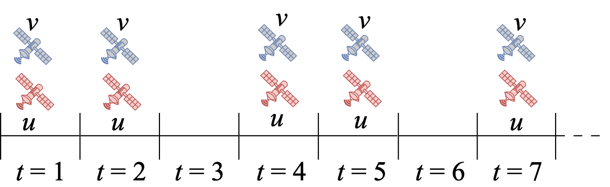
The introduced satellite network operates in a slotted, infinite time horizon, where denotes a time slot. We use the binary parameter (or ) to represent if the ISL between satellites and , referred to as -ISL, is active (or not). Due to the recurring nature of their orbits, satellites interact with each other at fixed intervals, and thus ISLs become active periodically as well. To model this periodicity, we introduce the following parameters; we assume that whenever the -ISL is active, it remains active for time slots before becoming inactive. In addition, denotes the period of -ISL (in time slots), implying that and , . Furthermore, we denote by the period of the entire network connectivity which can be computed as the least common multiple of . For simplicity, we assume that every data transfer between a satellite pair is completed within a single time slot using an inter-satellite free-space optical link with high transmission speed, long communication range, and high reliability. In this model, we only focus on the the sets of parameters and , to describe the network topology and motions of satellites for simplifying the presentation and enhancing the clarify. An illustrative example is provided in Fig. 1 with the presence/absence of the two satellites in a time slot implying an active/inactive ISL.
III-B SFCs, VNFs and Service Request Arrivals
As mentioned earlier, the satellites cooperatively execute computational tasks for certain types of applications. Each task requires data to be processed through the sequence of interconnected VNFs of an SFC. For instance, a wildfire detection involves several steps such as image processing, feature extraction, and fire classification [14], each one carried out by a separate function represented by a VNF in this work. An ordered sequence of VNFs comprises an SFC , where is the index set of all the available SFCs/services, . Also, we let be the set of all available VNFs. We denote by the VNF of SFC and by the set of VNFs comprising SFC . For a satellite to execute a specific VNF, the corresponding source code needs to be installed in the satellite’s computing system. The storage used for caching is excluded from the storage resources of a satellite. We denote by the pre-installed set of VNF types on satellite , with being its caching capacity. A VNF can only be placed/executed on satellite if . Due to their limited physical resources, it is not always feasible to install every available VNFs on the satellites. Therefore, we consider a scenario where a subset of VNF images has been pre-installed on each satellite. This means that , covering the unique case where .
At the end of time slot , a service request is initiated with a probability . A request initiation triggers satellite to request the placement of an SFC . We call this satellite the requester; and are the probability that satellite will be the requester and the probability that SFC will be requested, respectively, conditioned on the occurrence of a service request. A service request for SFC will expire at the end of time slot if not successfully served, where is the SFC’s end-to-end delay tolerance. In our system model, we assume that at most one SFC request is initiated per time slot. Additionally, since the execution of an SFC may span multiple time slots, a satellite can manage multiple requests within a time slot, including its own and those forwarded from other satellites. In this work, each request is assigned a timestamp (described in Section IV-B) corresponding to its initiation time, and requests are processed in ascending order of these timestamps. In a practical context where a satellite initiates or receives multiple requests with the same initiation time slot, these requests can be buffered to eliminate their temporal overlap. Each buffered request is processed in a time slot, and the proposed framework in this paper remains applicable. Timestamps along with the use of buffers help determine the order in which requests are processed, thereby preventing resource conflicts.
III-C VNF Execution and Inter-Satellite Data Transfer
We use the terms placement and execution interchangeably throughout this work. Executing SFC means that all the VNFs for are executed in the given order. That means the output of the VNF becomes the input of the VNF in the sequence. The output of the last VNF in the sequence bears the results carried out by SFC and needs to be returned to the requester satellite to mark the request as successfully served. We also denote by and the computational and storage resources required to execute and store its output.
We assume that if satellite executes VNF , and VNF is assigned to another satellite following a placement policy (e.g., because has not been pre-installed on ), needs to store the output of in its storage before forwarding111The forwarding path may consist of multiple satellites as relays. it to satellite . In this case, when has been executed, computational resources on satellite are released, but storage resources are consumed to temporarily store its output. That happens because the communication can occur only when the -ISL is active. After forwarding the data, storage resources are released on satellite , while storage resources are consumed on satellite to store the received data. That means that data forwarding might fail if the receiving satellite does not have sufficient available storage space. On the contrary, if a satellite is executing a sequence of VNFs, the intermediate data is not stored in its storage.
In this work, we address the following two sub-problems:
-
•
The first sub-problem is to assign VNFs to satellites and define data routing paths to optimize the overall system performance. We refer to this as the VNF/service placement problem which is formally defined and solved in Section IV.
-
•
The second sub-problem is to define the optimal VNF subset installed on each satellite. We refer to this as the VNF caching problem which is formally defined and solved in Section V.
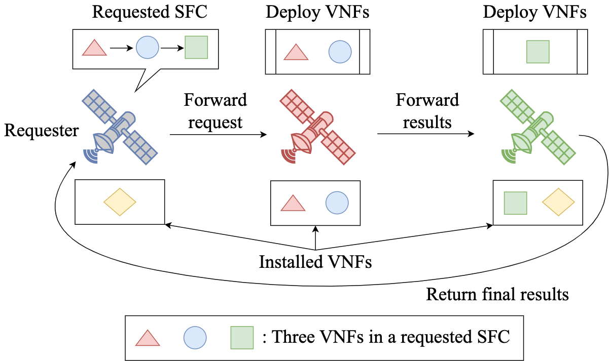
Fig. 2 illustrates a VNF placement constrained by installed VNF subsets. Table I summarizes the main notation. To reduce complexity, we will gradually augment the notation with additional variables as needed. In addition, we note that service requests and ISL transitions occur in each time slot. The former, along with the available resources of each satellite, constitutes the system state, which will be defined in the next section. The latter is due to satellite motions. Therefore, a time slot can be interpreted as a unit of time that quantifies both components.
| Notation | Description |
|---|---|
| Set of LSN’s satellites | |
| -ISL state at time slot , | |
| Active ISL duration, period, system period | |
| Computational, storage capacity of | |
| Set of LSN’s available SFCs/services | |
| Set of VNFs comprising SFC , with ( being SFC’s length) | |
| Set of cached VNF types on satellite , | |
| Service request, requester satellite, , and requested SFC, , probabilities | |
| SFC end-to-end delay tolerance | |
| computational, storage requirements | |
| execution delay on | |
| (DP) SFC placement | |
| Set of satellites that handle the request at each time slot | |
| Set of time slots where VNF is activated | |
| Largest end-to-end SFC delay tolerance | |
| Computational resource of | |
| Storage resource of | |
| (DP) System state: , , requested SFC , requester | |
| (DP) Transitioned system state | |
| (DP) State transition probability given | |
| (DP) Cost of placement on state | |
| Set of requests in the buffer of satellite | |
| (MAQL) Request handled by satellite , , , , | |
| (MAQL) Satellite state, | |
| (MAQL) Satellite actions, | |
| (MAQL) Cost when satellite performs action on handled request | |
| The set of available actions for request of satellite | |
| (MAQL) Placement policy | |
| (MAQL) Total cost of satellite for state and action sequence | |
| Order of current time slot in system period | |
| Q-table of satellite | |
| Q-value , and | |
| Learning rate and discount factor | |
| System-wide VNF caching strategy | |
| Request serving rate under policy and caching strategy | |
| Predicted mean, standard deviation, kernel function for caching strategies | |
| Acquisition function for caching strategy |
IV VNF Placement in LSNs
IV-A Dynamic Programming Formulation
The execution of an SFC can span several time slots, and its VNFs can be activated in multiple satellites at different time slots sequentially. We define the service placement as a tuple that contains both the indices specifying which satellites will handle data relaying and which will execute VNFs of the requested SFC, as well as their activation time slots. We denote it as , where:
| (1) |
and denotes the index of the satellite that handles the request at the time slot, with representing the time slot when the placement is performed. and are, respectively, the indices of the requester and the last satellite handling the request before the final result is obtained by the requester. We note that, by “handling” we refer to one of the followings: forwarding, carrying, rejecting a request or executing a VNF in it. Thus, calculating the number of elements in , i.e., , gives us the end-to-end SFC/service execution and data transfer time, in time slots, for placement . Set is defined as:
| (2) |
where is the time slot that VNF is activated, with representing again the time slot when the placement is performed. A request rejection is represented by . A simple and intuitive example follows:
Example 1
The requester satellite requests SFC comprised of two VNFs, and . We assume for simplicity that and , i.e., the first and second VNFs are cached on satellites and , respectively. It is also assumed that each satellite requires one time slot to execute its VNF. A feasible service placement is:
-
•
: Satellite executes .
-
•
: Satellite forwards its output to satellite .
-
•
: Satellite receives the data and executes .
-
•
: Satellite forwards the results back to satellite , the requester.
This placement spans time slots. From definition, we have that , and , as the two VNFs are deployed at and , respectively.
We note that when a placement is made at time slot , the required resources of all involved satellites in future time slots are reserved accordingly. We define as the largest end-to-end delay tolerance among all supported SFCs. We represent the system’s state by which is updated at the beginning of every time slot; encapsulates the satellites’ available resources for up to future time slots, the index of the requested SFC, as well as the index of the requester satellite.222It is sufficient for to convey time slots from the current one because no placement can span more than time slots. The vector of available resources of satellite for the next time slots is given by , with , where and are the available computational and storage resources of satellite , respectively, at time slot . These allow us to formally define the system state as:
| (3) |
where and are the indices of the requested SFC and the requester at the end of the previous time slot, respectively. If there is no request in the previous time slot, .
We define as the transitioned system state resulted by placement in the beginning of the following time slot; represents the transitioned vector of available resources on satellite . We compute the components of as follows:
-
(i)
if and , meaning that satellite is executing VNF , hence, . Therefore, , and , .
-
(ii)
else if , , and such that either or , meaning stores the output of . Therefore, and . We note that if , with , then .
-
(iii)
else either , i.e., satellite is not part of the placement , then, , , or the placement spans less than time slots (), then, , .
Since a valid placement cannot span more than time slots, , and always. A representative example is provided below to aid the understanding of the definitions of system states and state transition:
Example 2
Let us consider an LSN consisting of two satellites, , where each one is equipped with computational resources equal to and storage resources equal to . Two services are offered by the system as SFCs, , of length and maximum end-to-end delay tolerances equal to and time slots. We have . The execution of each of their VNF components consumes computational resources and requires , , time slots to complete. Their output consumes storage resources when stored. Data forwarding takes time slot. Let and , i.e, the two satellites are in the communication range of each other every time slots and once they are connected, their connection remains active for time slot. Initially, we assume that the two satellites are not connected, i.e., the -ISL is inactive, thus , while they have all their resources available, i.e., and for . Additionally, let and , i.e., satellites 1 and 2 come pre-installed with the second and the first VNF of SFC , respectively.
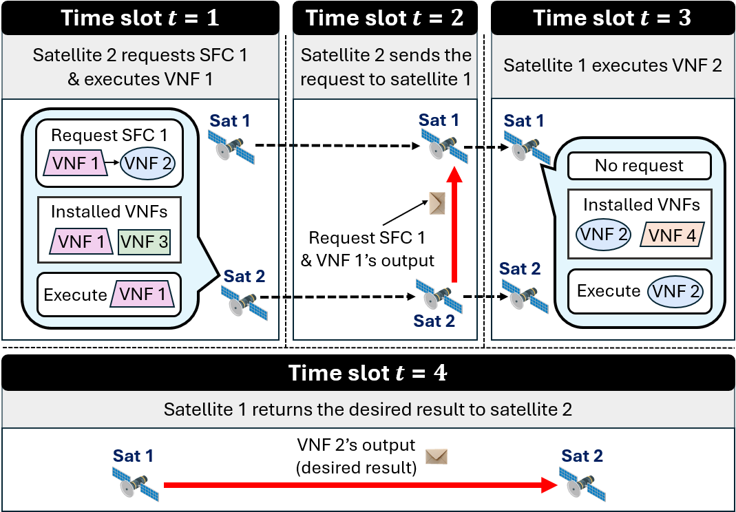
At the end of time slot , the requester satellite initiates a service request for SFC . Then, the system state at the beginning of time slot is , where and . We visualize a feasible service placement of this example in Fig. 3, with the following details:
-
•
: Satellite 2 executes which has been installed.
-
•
: Satellite 2 forwards its output to satellite 1.
-
•
: Satellite 1 receives the data and executes .
-
•
: Satellite 1 forwards the output of (the desired result) back to satellite 2, the requester.
From this process, we obtain and . We can calculate the components of the transitioned vectors of available resources , , through the following steps:
-
•
For with , condition (i) is satisfied. The same stands for with . Therefore, and .
-
•
For and such that , condition (ii) is satisfied. The same stands for . Therefore, and . Also and .
-
•
Since the placement spans time slots, condition (iii) is satisfied for calculating the rest of the components. Therefore, and , . Finally, and .
Next, we define the transition probability from to , given a placement , as:
| (4) |
Additionally, we define the system cost for performing placement , while on state , as: if the request is served, and if rejected.
To accommodate the calculation of the long-term, time-dependent discounted cost, we augment the state and placement variables with time slot notation, and , respectively. Then, this discounted cost can be given by:
| (5) |
where is the discount factor. The objective of the VNF placement task is to minimize the discounted cost (5). Let be the minimum discounted cost which can be calculated through the following DP Equation:
| (6) |
Solving (6) produces the optimal service placement that minimizes the end-to-end delay for the requested service.
A valid placement adheres to the system constraints. We remind that , with and having been defined in Eqs. (1) and (2) respectively. denotes the index of the satellite handling the request in the time slot and denotes the time slot at which the VNF is executed; denotes the current time slot. Therefore, is the index of the satellite executing the VNF. Then, the set of VNF placement constraints with respect to (wrt.) the requested SFC is given as:
| (7) | |||
| (8) | |||
| (9) | |||
| (10) | |||
| (11) |
Constraint (7) guarantees that the end-to-end delay of the placement does not exceed the maximum delay tolerance of SFC . Constraint (8) ensures that the satellite executing VNF at time slot has sufficient computational resources. Constraint (9) ensures that every satellite handling the request has enough storage resources to store VNFs’ outputs. We note that before the first VNF is executed, only the request event is transferred between satellites, with no intermediate data produced by VNFs; hence, storage resource is considered to be unaffected and the constraint (9) is not required for . Constraint (10) ensures that only satellites installed with VNF can execute this VNF. Finally, constraint (11) guarantees that data is transferred only via active ISLs. Additionally, we note that if , then always.
IV-B Multi-Agent Q-Learning Solution
Finding a solution for the DP Eq. (6) subjected to constraints (7)-(11) can be computationally intractable due to its recursive nature. Furthermore, this equation assumes knowledge of the probabilities associated with service requests, i.e., , , and , which are typically unobtainable in a realistic environment. To tackle this challenge, we reformulate the VNF placement problem as an MAQL model. In this context, each satellite operates as an independent agent with the goal of learning the optimal VNF placement policy for a requested service. The components of the MAQL model are defined as:
IV-B1 Agent’s State
The agent’s state of a satellite in a time slot , describes its available resources and the SFC requests it is currently handling. This state is derived from the system state , introduced in the previous section for the DP formulation. We note that although only one request arrives at the system per time slot, each satellite might be handling multiple requests at each given moment. An agent’s state is defined as follows:
| (12) |
where and are the available computational and storage resources at satellite , respectively, in the considered time slot, is the set of requests handled by satellite at the considered time slot, and is the number of its elements; is the handled request from the set of requests handled by satellite and is defined as:
| (13) |
where and is the augmented requested SFC and requester satellite notation for the specific request, respectively; represents the timestamp that indicates the initiation time slot of the request. We assume that the requests are stored sequentially in the agent’s state, i.e., if , then . indicates the next VNF in SFC that needs to be executed. When exceeds the total number of VNFs in SFC , i.e., , all the VNFs of the requested SFC have been executed and the final result is to be returned to the requester. An example follows:
Example 3
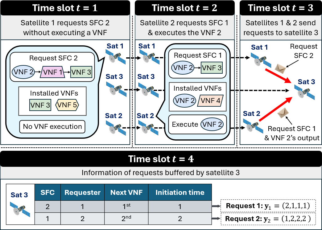
We consider two SFCs with the following topologies; SFC 1: VNF 2 VNF3 and SFC 2: VNF 2 VNF 1 VNF 3. The execution of each VNF in these SFCs spans time slot. The following scenario takes place:
-
•
: Satellite requests for SFC 2, and carries the request over to the next time slot due to inactive ISL.
-
•
: Satellite requests for SFC 1 and executes . Satellite again carries the request over to the next time slot.
-
•
: The - and -ISLs of the considered satellites are active. Satellite forwards the request for SFC 2 to satellite , without executing any VNF. Satellite also forwards the request for SFC 1 and the output of to satellite .
Therefore, at time slot , satellite is handling two requests and in ascending order of their initiation times. We present Fig. 4 to aid the intuition of this example.
IV-B2 Agent’s Action
Each agent’s/satellite’s VNF placement action at a given time slot is a set of sub-actions, each directed to one of the requests it is currently handling:
| (14) |
where is the sub-action concerning handled request . We remind that the request index is assigned following ascending order of request initiation time. Based on that, request is handled before request , i.e., decision is taken before . We identify possible sub-actions for each request and classify them into four categories denoted by , and as follows:
-
•
(A1): ; forward the request to satellite . This sub-action is valid if the followings hold: (i) the -ISL is active at the current time slot, and (ii) if , , i.e., satellite has sufficient storage resource to receive the request.
-
•
(A2): ; execute VNF . This sub-action is carried out, provided that the following three conditions are satisfied: (i) not all the VNFs of SFC have been executed, i.e., ; (ii) the said VNF is pre-installed on satellite , i.e., ; (iii) the satellite has sufficient available resources.
-
•
(A3): ; reject the request (always valid).
-
•
(A4): : stall and carry the request over to the next time slot (always valid).
Let be the family of valid actions of for request . In this MAQL setup, we determine a VNF placement policy, denoted by , as a rule that maps each request to an action .
IV-B3 Instant Cost
By performing sub-action for a request , a cost is induced on satellite , depending on the the type of sub-action:
where is the indicator function which is equal to if the enclosed condition is satisfied and otherwise. In detail, if satellite forwards the request to satellite and has enough available storage to receive it, then, the induced cost is equal to the transferring time ( time slot). Otherwise, data cannot be received, and a penalty is incurred. In case satellite executes this part of the handled request, the cost is equal to the VNF’s execution time. Rejecting a request costs a penalty equal to . Finally, stalling and carrying a request over to the next time slot incurs a cost equal to . Given a satellite’s state , we define the total cost for induced for performing a sequence of sub-actions, i.e., action as:
| (15) |
IV-B4 Learning Mechanism & Optimal Action Estimation
In the following, we augment the agent’s state, handled request and agent’s action notation to accommodate time slot locality, as , and . We additionally drop the satellite, , and sequence, , subscripts from them, to avoid overloading the equations. Given the above, in the MAQL environment we are defining, each satellite aims at learning the optimal VNF placement policy that minimizes the following discounted long-term cost:
| (16) |
where , being the sub-action for request dictated by policy . Approximating the optimal policy is equivalent to approximating an action for every request in each time slot that minimizes this discounted long-term cost.
In our MAQL framework, the Q-table contains the approximations of the long-term sub-costs . Let be the Q-table of satellite that stores all the learned Q-values. We remind the reader that the network topology varies deterministically and periodically with a period . Therefore, at a time slot , the network topology and its upcoming changes are the same as those at a time slot , where . This time slot then can be computed wrt. as , where returns the remainder of . To this end, we denote by the Q-value estimation of cost . For presentation convenience we fix the time slot thus hereafter the notation is dropped.
In this setting, each satellite’s environment is non-stationary as it depends on the policies employed by other satellites which continually evolve, meaning that system convergence is not guaranteed. To address this concern, we promote collaboration among the agents in the form of knowledge sharing. When satellite forwards a request to satellite , shares its learned Q-values as follows:
-
•
If satellite has handled the request before, i.e., the row is populated on , then the value is shared with satellite .
-
•
Otherwise, a predefined initial Q-value is shared.
Let . Having acquired shared Q-values from other satellites, satellite updates each component if as follows:
| (17) |
where if ; if . , are the learning rate and the discount factor, respectively; is the next state of , where: (i) if , (ii) if . If , the request is rejected and the penalty cost is yielded: . Then, satellite approximates its optimal action for a handled request by:
| (18) |
A formal description of the MAQL-based VNF placement method is provided in Algorithm 1.
Mapping the policies , resulted from the convergence of the MAQL algorithm, back to , allows us to define as the VNF placement policy that minimizes end-to-end delay for the requested service.
Remark 1. (MAQL Framework’s Features Supporting Large-Scale LEO Satellite Systems): In mega-constellation LEO satellite networks, the decentralized architecture of the MAQL framework facilitates scalability and reduces the need for extensive global coordination. Furthermore, parameter sharing mechanism enhances both scalability and learning efficiency within large networks.
V VNF Caching in LSNs
In the previous sections, we assumed that each satellite comes pre-installed with a subset of VNFs. Based on this, VNF placement is carried out. In this section, we aim to determine the optimal subset of VNFs to be cached/pre-installed on each satellite, thereby maximizing the successful request serving rate.
V-A Objective Function Formulation
We recall that is the given, fixed caching capacity of satellite . A system-wide caching strategy is given as:
| (19) |
where contains the VNFs cached by satellite , and are those cached by satellite 1. The objective of the VNF caching task is to maximize the average number of requests served in a time slot, i.e., the request serving rate. Thus, we aim at maximizing the objective function where is the expectation operator; is associated with the VNF placement policy and caching strategy , as:
| (20) |
where is a predefined time horizon for calculating the serving rate and is the VNF placement at time slot , following policy , given the VNF caching strategy . Our objective is then to calculate the optimal caching strategy that maximizes the expected request serving rate:
| (21) |
V-B Bayesian Optimization Solution
Bayesian Optimization (BO) is a powerful iterative method for optimizing black-box functions [22]. This subsection outlines the key components and the BO-based algorithm for solving Eq. (21).
V-B1 Search Space
We define our solution search space as the family of caching strategies that satisfy the following conditions: i) there exists at least one SFC such that and ii) a VNF is not cached more than once in each satellite.333In executing multiple VNFs, a satellite can access simultaneously access all installed VNFs. Hence, it is sufficient to cache a VNF once. The first condition ensures that at least requests for one type of SFCs can be served, and the second guarantees that no caching storage is wasted.
V-B2 Surrogate Model
A probabilistic, surrogate model is selected and trained to predict the distributions of the objective function’s outcomes, defined in Eq. (20), for various inputs . Let and be the predicted mean and standard deviation for , respectively. Let also the radial basis function serve as the kernel function, which is responsible for measuring how close the VNF caching strategy is to the training data, where is a predefined length scale parameter and . We select the Gaussian Process (GP) as our surrogate model based on the following considerations.
First, defined in Eq. (20) is a summation of the indicator functions, the outputs of which are random quantities. Then, when is sufficiently large and the outputs of the indicator function are weakly dependent, the Central Limit Theorem [23] can be applied. This theorem suggests that, under these conditions, the distribution of will approximate a normal distribution.
Second, GP modeling offers computational tractability. Let be an input strategy for which has been evaluated. We call a training data point, and the training dataset. Under the GP modeling, we have the prior distribution where is a matrix consisting of elements , . For a family of non-evaluated strategies , the joint distribution between and can be expressed as:
that provides analytically tractable expressions for the marginal and conditional distributions. The posterior distribution, i.e., the predicted distribution of non-evaluated strategies , given the training dataset , follows a Gaussian distribution, , where:
| (22) | |||
| (23) |
, and being a non-evaluated caching strategy and being a strategy from the training dataset. The obtained posterior distribution is used to predict the mean and variance of . The current posterior distribution is then considered as prior in the following iteration.
V-B3 Acquisition Function
The role of the acquisition function in the BO is to guide the search for the optimal solution in the search space [22]. To come up with the most efficient way of doing so, we implemented and evaluated the following four acquisition functions:
a) Probability of Improvement (PI): this function provides an exploration-exploitation balance metric for guiding the search process by estimating the likelihood that a new sample will surpass the current best observation, . The PI function is defined as:
| (24) |
where is the Cumulative Distribution Function (CDF) of the standard normal distribution.
b) Expected Improvement (EI): this function measures the expected improvement over , when evaluating a candidate input strategy , and is defined as:
| (25) |
c) Upper Confidence Bound (UCB): This function aims to balance exploration and exploitation by considering the uncertainty associated with the objective function’s evaluations and is given by:
| (26) |
where is a predefined parameter that controls the trade-off between exploration and exploitation.
d) Lower Confidence Bound (LCB): This function aims to maximize the lower estimate of the objective function’s evaluations and is defined as:
| (27) |
LCB tends to exploit the known regions of the search space more aggressively.
V-B4 The BO Algorithm
We initiate the process by constructing the training set ; Depending on the size we are opting for, we repeat a random selection of candidate caching strategies from the search space, for evaluation; is calculated by caching the VNFs on satellites according to , letting the system run for time slots following the VNF placement policy , and counting the number of successfully served requests. Naturally, this makes the evaluation step a time-consuming process. Therefore, during the BO runtime, we only evaluate caching strategies that have the potential to be the optimal solution, , guided by the acquisition function:
| (28) |
We then evaluate the objective function and update the surrogate model; the prior distribution of is updated to a posterior Multi-variate Gaussian Distribution, with a mean value and a kernel matrix given by Eq. (22) and (23), where now is the training dataset augmented by , the last evaluated input strategy.
After running the above steps for a sufficient number of time slots and candidate optimal solutions , the optimal VNF caching strategy is calculated as:
| (29) |
In practice, each satellite obtains the VNF caching data from the controller on the ground and installs the VNFs dictated by . We envision this step as a one-time pre-online task. However, the learning process can continue to operate in the background, during runtime, seeking potential improvements in the VNF caching strategies. Each newly discovered and superior solution can be seamlessly applied, leading to an iterative refinement process. We concisely and formally present the discussed BO-based VNF caching method in Algorithm 2.
In addition, we note that the proposed VNF placement and the caching frameworks are dependent on each other. The optimal solution is obtained by executing the two processes of caching and placement in an iterative fashion. The BO-based algorithm presented in this subsection serves as an outer layer that provides the caching strategy that needs to be evaluated. The MAQL-based VNF placement policy, which serves as an inner iteration, returns the optimal serving rate after convergence. As we iterate, we obtain an optimal caching strategy and a converged MAQL model associated with this strategy.
VI Numerical Results
In this section, we assess the performance of the introduced VNF placement and caching algorithms. In this framework, we utilize the concept of time slots to discretize the transition of state (defined in Eq. (12)) and the motion of every satellite where the latter factor leads to the intermittency of ISLs. For the simulations, the default values of the common parameters are given in Table II. Variations in these or other parameters will be noted in each simulation. The details of the considered SFCs are given in Table III with time slots, . The required computational and storage resources are given as follows:
-
•
SFC 1: and for .
-
•
SFC 2: and for .
-
•
SFC 3: and for .
-
•
SFC : and , .
| Parameter | Value |
|---|---|
| 1 time slot | |
| , , | 0.9, , |
| 1 time slot | |
| , , | 100, 0.6, 0.6 |
|
|
VI-A Cooperative MAQL-based VNF Placement
First, we evaluate the efficiency of the MAQL-based VNF placement mechanism. The optimal placement is given by the DP Eq. (6). To calculate the average cost, we compute the discounted long-term cost using Eq. (16). Additionally, the serving rate is determined by dividing the number of successfully served requests by the total number of requests. The learning rate is and decreases to 0.01 if there is no improvement in a certain period of time.
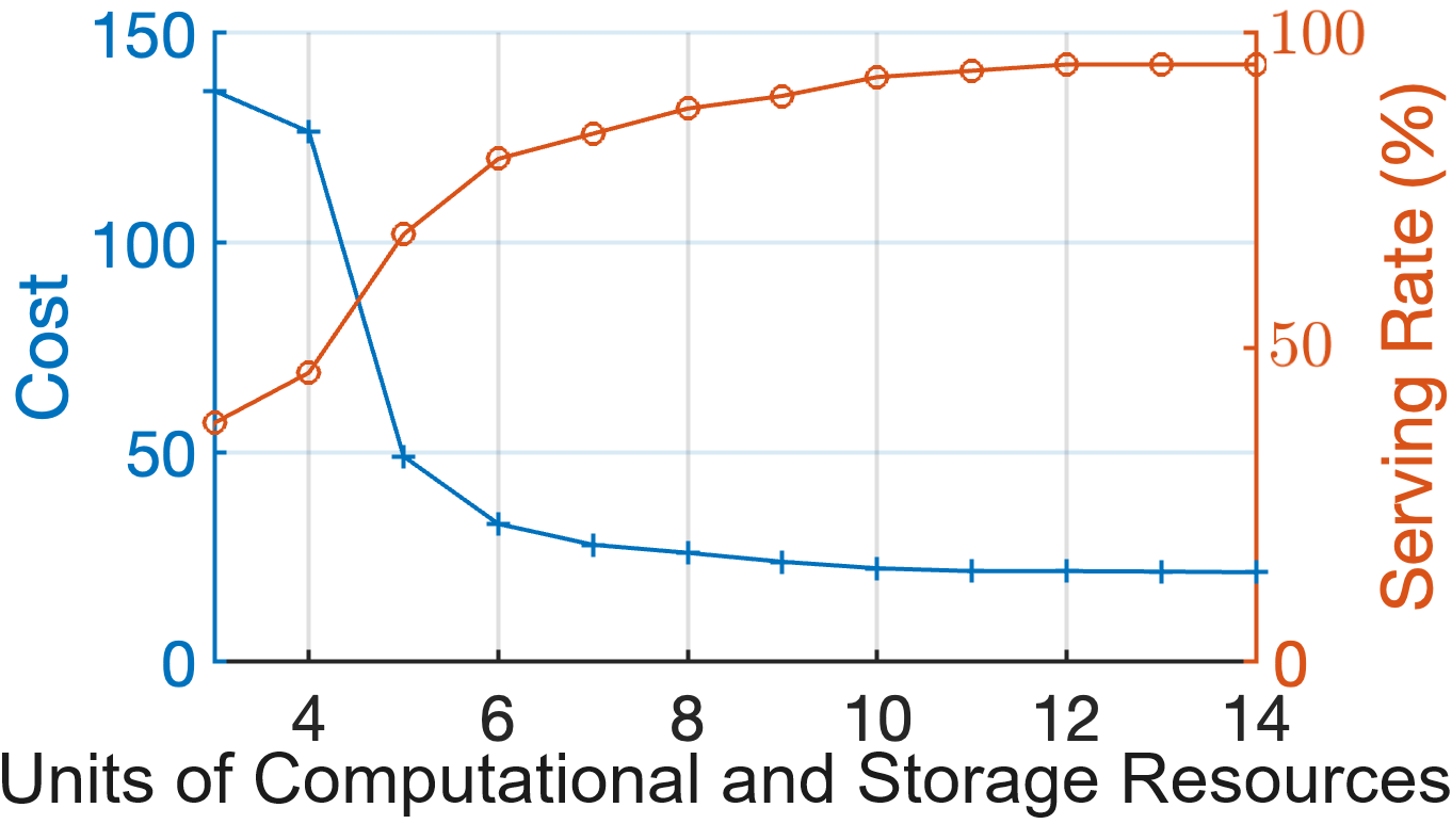
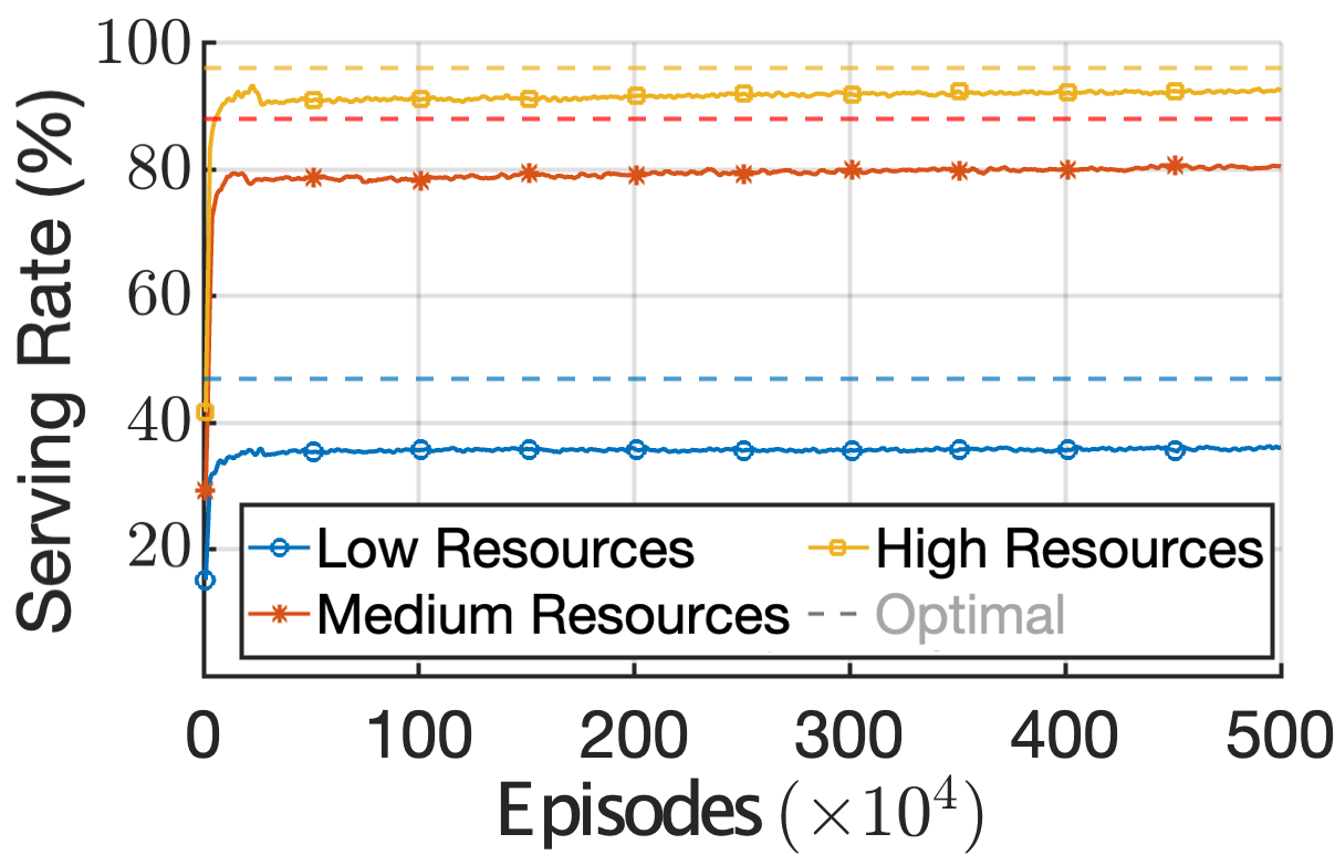
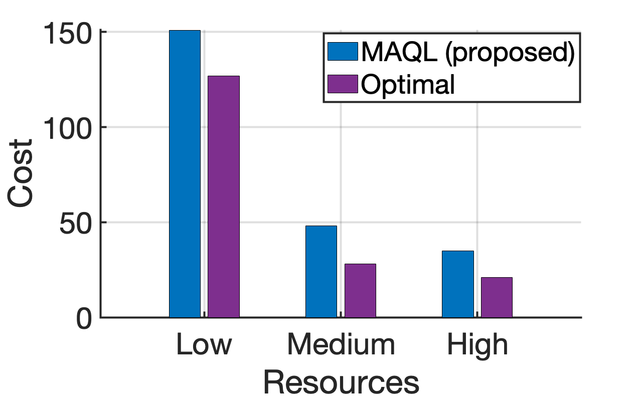
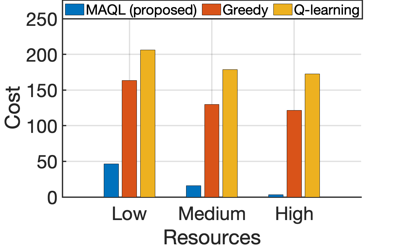
1) Performance against the Optimal solution: We compare the proposed scheme against the optimal in Fig. 5. Our simulation setup involves satellites, and a set of available services . The sets of VNFs cached on the satellites are given as , and , respectively. The active ISLs periods between satellites are , and time slots. The number of computational and storage resource units are equal, , . To set the reference point, Fig. 5(a) presents an analysis on the optimal discounted long-term cost and serving rate achieved through the proposed DP Eq. (6); as expected, the cost decreases and the serving rate increases as the satellites become more resourceful. Next, we define three levels of available satellite resources, Low, Medium and High, where , 7 and , respectively. Having established the optimal behavior, in Fig. 5(b) we compare the proposed MAQL approach against it; we observe that the proposed VNF placement solution quickly converges to near-optimal serving rates for all cases. Nonetheless, the more the initial satellite resources, the better the performance as the solution search space becomes broader. Similar observations can be made from Fig. 5(c), where the long-term system cost achieved after convergence is shown to be close to the optimal. We note here that throughout the experimentation under the Low satellite resources, of the times the placement policy had VNF executed on satellite and of the times on satellite ; this preference on satellite is a result of the resource contention for the limited resources of satellite . We should also note that after the one-time offline training of the algorithm, inferring the best policy is instantaneous; in this simple setup, the online execution time is on average for MAQL, while the optimal DP-based solution requires to calculate a solution, making it unfit for real-time decision making.
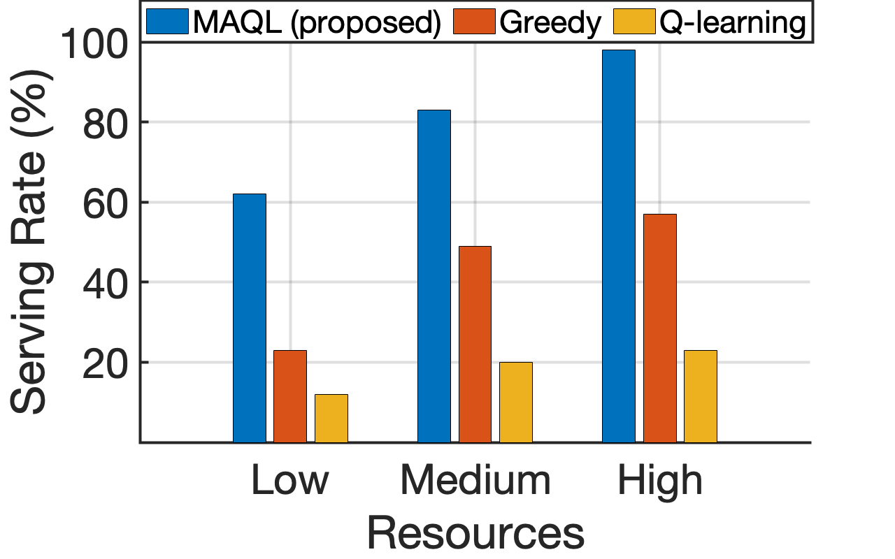
2) Performance against baselines and impact of the satellite number: We then assess the proposed algorithms against two baselines and illustrate the impact of a growing number of satellites in Fig. 6. Here, we assume a system with the SFC set and satellites grouped in two subgroups: and . The active ISL periods are if or , otherwise. The sets of cached VNFs are given as , , , , and . A brief description of the compared baselines follows:
a) Q-learning [24]: we modified this learning VNF placement algorithm for an LSN environment as follows:
-
•
State: the requested SFC and VNF for execution.
-
•
Action: the satellite that will execute the above VNF.
-
•
Reward: , where and are the ratios between the required/available computational and storage resources on the designated satellite, respectively; is the end-to-end delay of the SFC placement, and is the length of the SFC. Other parameters values are as in [24].
We note that this Q-learning-based method is a centralized method that makes a placement decision for an entire SFC in a single time slot, based on the set of active ISLs.
b) Greedy [25]: We modify this work’s mechanism to fit our LSN environment by matching our requester satellite concept with both the ingress and the egress switch since the data must be returned to the requester. Based on this, a satellite selects another satellite to transfer data by assigning them a cost score. The original cost function is altered as follows: where is the delay for transferring data from satellite to , which consists of the waiting time for the -ISL and the transferring time ( time slot). A satellite will transfer the data to satellite with the earliest ISL availability (if more than one, it selects randomly uniformly). The VNF placement is performed step by step in each time slot.
To make a fair comparison, none of the three algorithms have knowledge of the pre-installed VNFs at the beginning of the experiment. Figs. 6(a) and 6(b) illustrate the results of this benchmarking, in terms of achieved serving rate and cost. The MAQL-based solution outperforms the alternatives by allowing satellites to share learning parameters, enabling cooperative policy updates toward optimal solutions. The Greedy method prioritizes shorter paths while it transfers data between satellites without any VNF caching knowledge, resulting in longer end-to-end delays. Although the high end-to-end delay tolerance in our setting allows data to eventually reach a satellite with the requested VNF cached, stricter tolerances would further degrade the Greedy approach’s serving rate. On the other hand, although the plain Q-learning method can eventually learn the VNF caching information, it yields a lower performance compared to the Greedy scheme; this mechanism does not consider the ISL periodicity, meaning that data can be transferred during an inactive ISL, deeming the placements invalid.
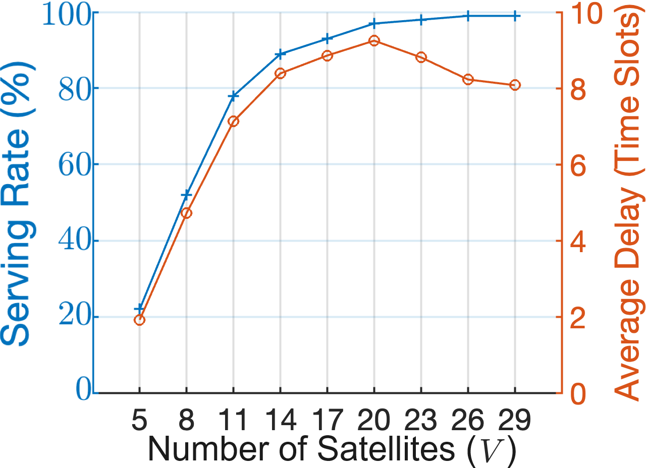
Subsequently, we examine the influence of the number of available satellites on the proposed VNF placement scheme’s performance. The satellites are divided into three subgroups: contains the first satellites, contains the next satellites, contains the rest, with . ISLs are always active within a subgroup, and intermittent between subgroups with the following periods: if none of and belongs to ; if either or belong to . Each satellite has units of available resources and is installed with one VNF. We investigate such a limited-resource scenario in order to emphasize the impact of the topology expansion as the number of satellites, , increases. SFCs are considered with (details available in Table III) which comprise VNFs. The VNF execution time is fixed at 2 time slots, i.e., . VNFs are selected and installed in the satellites in a round-robin fashion. The results are presented in Fig. 6(c). There, we observe that in terms of request serving rate, the performance increases significantly (from to almost 100%) when more satellites are available, due to the increased resource and caching capacity. The right y-axis of Fig. 6(c) presents the average end-to-end service delay calculated by dividing the total induced delay by the total number of requests, including successfully served and rejected ones. When is small compared to the number of VNFs (e.g., ), there might not be enough VNFs installed in the network to form the entire requested SFC. However, a satellite might still execute an (installed) VNF and transfer the results to another satellite, causing a small delay before the request is rejected (e.g., around 2 time slots for ). This occurs because the satellites are not aware of the installed VNFs and resources of each other. Naturally, the larger the is, the more complete sequences of SFCs can be deployed, resulting in an increase on average delay alongside the serving rate. On the other hand, as increases, , and also increase, allowing for more VNFs to be installed in each subgroup. This, in turn, increases the probability for an SFC to be deployed as a whole within a single subgroup where ISLs are always active. This further reduces the deployment time by avoiding the waiting time for ISLs. As a result, after the sweet spot of where the serving rate is maximized, the average delay starts decreasing from to time slots per request.
3) VNF placement with large-scale service request: We now extend our analysis to a large-scale service request context, introducing increased randomization in the service request events. In particular, the set of VNFs is , and a random requested SFC is generated via Algorithm 3 where the input distributions and are Uniform Distributions. The total number of SFCs in the sample space of Algorithm 3 is computed by: SFCs. We consider a setup with satellites separated into three subgroups , , and . The available computational and storage resources are given by units. We let be the maximum length of a requested SFC, and consider three different scenarios where , 8, and 10, respectively. Intuitively, the greater the length of a requested SFC, the more resource units and time slots are required for the deployment. Also, we set and time slots, , as the delay tolerance of SFC and VNF execution duration, respectively. ISLs in the same subgroups are always available. if neither nor is in and if either or is in .
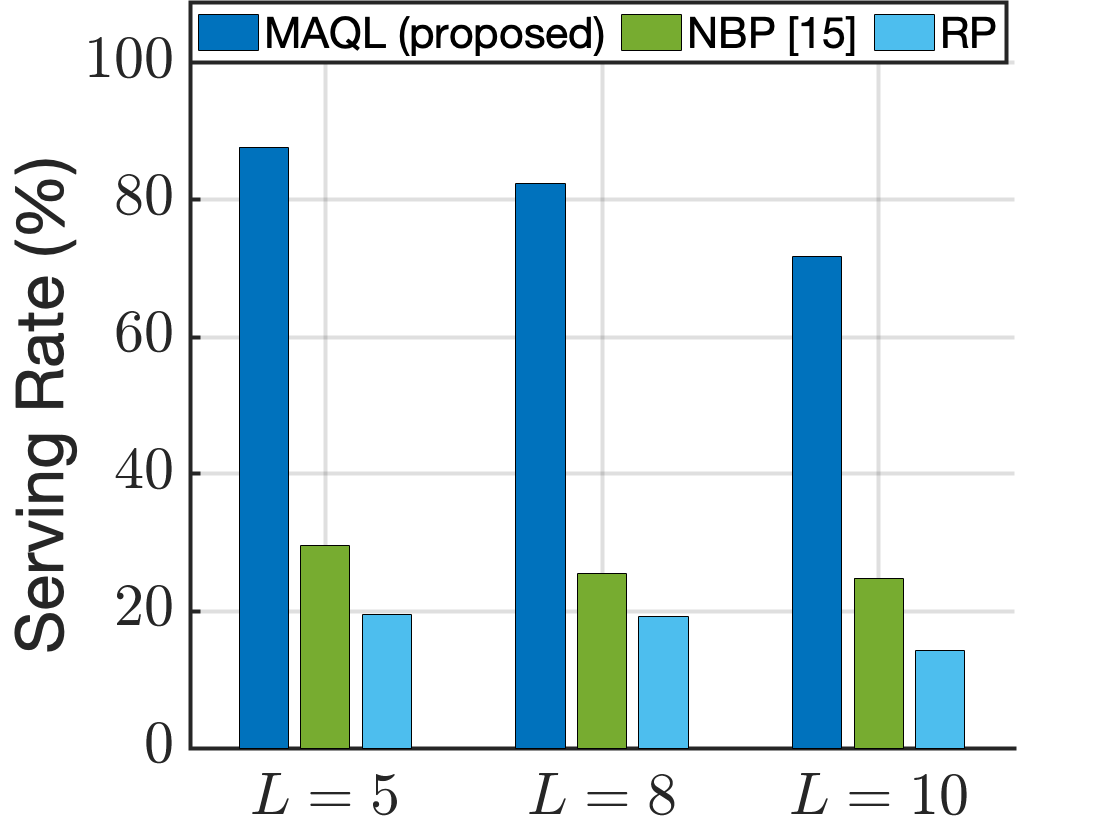
We compare the proposed MAQL-based scheme against the Neighbor-Based Placement (NBP) scheme proposed in [15]. Originally, in [15], placement decisions for all VNFs in the requested SFC are made simultaneously, and only available ISLs and resources at the placement time are considered. A request is rejected if no satellite in the sub-network can execute it. To make the comparison fair, we modified the NBP method as follows: satellites can only execute VNFs cached on them, and requests are rejected with a penalty incurred if either the resources are insufficient or the required VNFs are not cached. Additionally, the Random Placement (RP) scheme is also considered as a baseline in which a satellite selects an action uniformly randomly for each request in its buffer.
Our results are in Fig. 7. The MAQL-based scheme shows a superior serving rate compared to the NBP scheme. This advantage arises because the proposed approach allows satellites to handle one SFC deployment step per time slot, leading to more effective use of future ISLs and resources. Although the NBP scheme optimally places VNFs under the given constraints, its performance is significantly limited by the requirement that satellites can only execute installed VNFs. This restriction, which relies solely on currently available satellites, severely reduces the number of executable VNFs. In contrast, the MAQL-based framework demonstrates a clear advantage in this context. Besides, the RP scheme, with a lack of strategic planning, shows lower performance compared to the others.
VI-B BO-based VNF Caching
In what follows, we evaluate the efficiency of the BO-based VNF caching mechanism. To simplify the evaluation of this component and to avoid any bias potentially induced by the MAQL-based VNF placement, we test the caching mechanism through the following straightforward, greedy VNF placement scheme: if a satellite has the required VNF cached, it executes it, otherwise, forwards the request to satellite with the earliest ISL availability, and which has the required VNF cached. It is assumed that every satellite has complete knowledge of the cached VNFs on every other satellite. For this experimentation family, we first utilize an infrastructure consisting of satellites and SFCs, specifically . We group the satellites into three distinct subgroups as follows: , , and , with . The ISLs between satellites of the same group are always active. The rest of the active ISL periods are given as: between satellites of and , between satellites of and and between satellites of and . Each satellite can cache at most two VNFs, i.e., , and their initial resource capacities are equal to , .
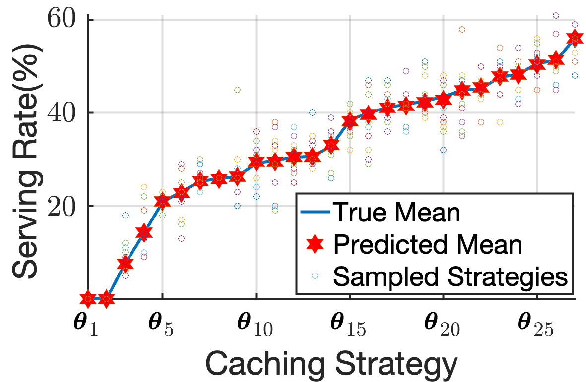
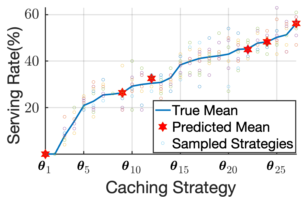
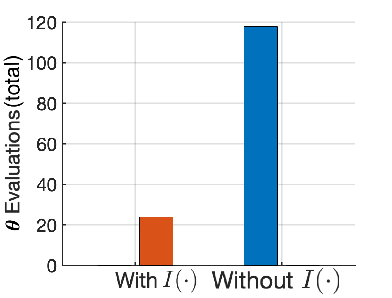
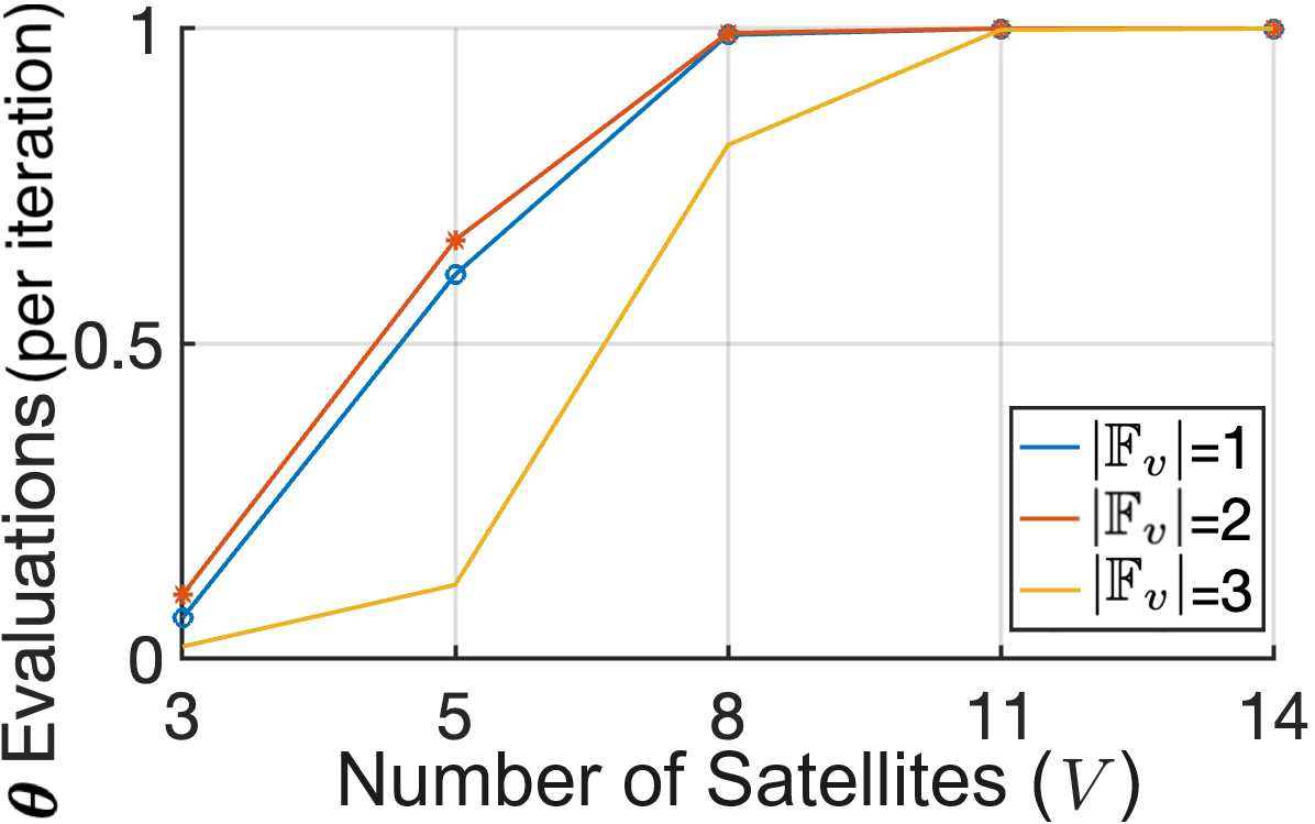
1) Performance impact of Acquisition Functions: We study the impact of incorporating an acquisition function in Fig. 8, by closely examining three satellites, one from each group , and . We employ the PI acquisition function, Eq. (24), in our proposed BO-based caching method to perform caching on three VNFs, . Given that , , this allows for choosing between three unique caching sets for each satellite, which gives us a search space of caching strategies. In the case where no is used, is sampled randomly from . The results of this case are illustrated in Fig. 8(a), where we observe that the GP model’s predictions align closely with the actual average serving rates represented on the x-axis for each caching decision. This emphasizes that the GP serves as a suitable surrogate model for our problem. However, without the guidance of an acquisition function, all the potential cache placements are subjected to evaluation, resulting in a considerable increase in execution time. Contrarily, when is calculated through an acquisition function as in Eq. (28), the number of evaluations required is significantly reduced, and the outcome approaches the optimal solution, showcasing a more efficient operation, as shown in Fig. 8(b). For visualization purposes, the caching strategies in Figs. 8(a) and 8(b) are sorted based on the true mean serving rate achieved with them. In Fig. 8(c), we illustrate the benefits of using an acquisition function; this reduction of in the number of evaluations needed directly translates to immense savings in real-world execution time. Specifically, in our setup, evaluating every potential caching strategy translated to total execution time, whereas the same optimal caching strategy was pinpointed through the acquisition function in just .
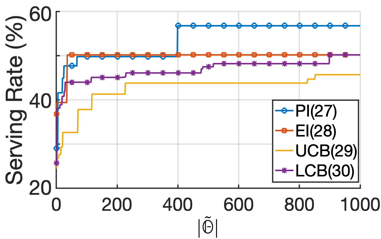
2) Performance impact of Acquisition Function type, cache size and comparison against baselines: In Fig. 9, we compare the performance of the four acquisition functions by analyzing the serving rate achieved as the training set size increases with each iteration of Algorithm 2. The superior performance of the PI function, Eq. (24), as illustrated in Fig. 9(a), suggests that in the VNF caching problem, exploration and prioritizing immediate improvements are dominant factors. PI places a strong emphasis on exploring regions of the search space where improvements are likely, and this approach evidently proved advantageous. On the other hand, the EI function, Eq. (25), which also prioritizes exploration but to a slightly lesser extent, provided consistently good results, though subpar compared to PI. Contrarily, the UCB Eq. (26) and LCB Eq. (27) functions emphasize exploration by considering upper and lower bounds on the evaluated function, but they do not directly measure the likelihood of improvement over the current best value. This undermines the significance of identifying areas with the potential for caching policy improvements, and this is reflected in the mediocre performance. This improvement of the serving rate in this function follows a step function pattern, as the best serving rate achieved is improved only when a better caching solution is found. Following, in Fig. 9(b) we demonstrate the results of benchmarking the proposed VNF caching mechanism (BO) against two baselines from the literature:
a) Coordinate Descent (CD) [26]: initialize the caching strategy and . In each iteration do:
-
(i)
Produce different caching strategies by alternatively assigning the component of with the VNF indices . Then, evaluate for every obtained .
-
(ii)
update to the with the maximum evaluation.
-
(iii)
.
-
(iv)
Return if termination criteria met, else go to (i).
b) Pattern Search (PS) [27]: initialize randomly. In each iteration do:
-
(i)
generate neighbor strategies ; is a neighbor of if there exists indices and such that , , and for . Evaluate for every obtained .
-
(ii)
update to the with the maximum evaluation.
-
(iii)
Return if termination criteria met, else go to (i).
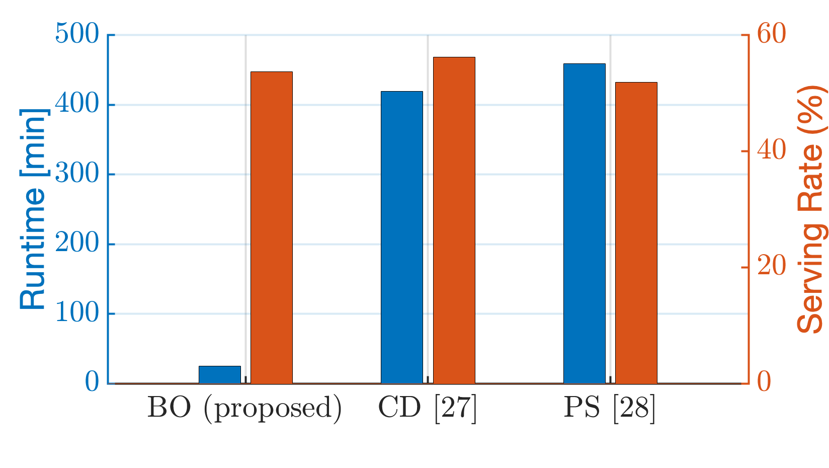
The results depicted in Fig. 9(b) indicate that the BO, CD, and PS schemes offer comparable serving rates upon completion. However, the BO scheme demonstrates a superior ability to strike a balance between maximizing the objective function and maintaining a low execution time compared to the other candidates. This is due to the ability of the presented framework in predicting the potential improvement of an unevaluated strategy. Finally, in Fig. 9(c) we briefly demonstrate the scalability of the BO-based algorithm. Since the objective function evaluation time accounts for the majority of the running time, we opted to show the average evaluations per iteration (lines in Algorithm 2) as the size of the infrastructure grows, for different cache sizes .
Next, we consider that results in 4 VNFs to be cached. Additionally, satellite subgroups are formed as follows: contains the first satellites, the next satellites and contains the rest. The ISL periodicity between the logical subgroups remains the same as defined at the beginning of this subsection. The figure suggests that the evaluation rate increases monotonically as the infrastructure size increases. This is consistent with the fact that the total number of caching strategies is given by . In addition, since the number of possible VNF subsets to cache on a satellite is given by the binomial coefficient we see that more evaluations are required when and and less for .
3) Assessing the combined performance of the MAQL-based VNF-Placement & the BO-based VNF Caching methods: In this simulation, we compare the proposed MAQL-based scheme with the NBP scheme [15]. For both schemes, the subsets of installed VNFs on the satellites are selected via the proposed BO-based algorithm. The setup in this experiment is as follows: and the network consists of satellites with , and being the periods of ISLs between the satellite pairs. The satellite resources and VNF execution time are given as and .
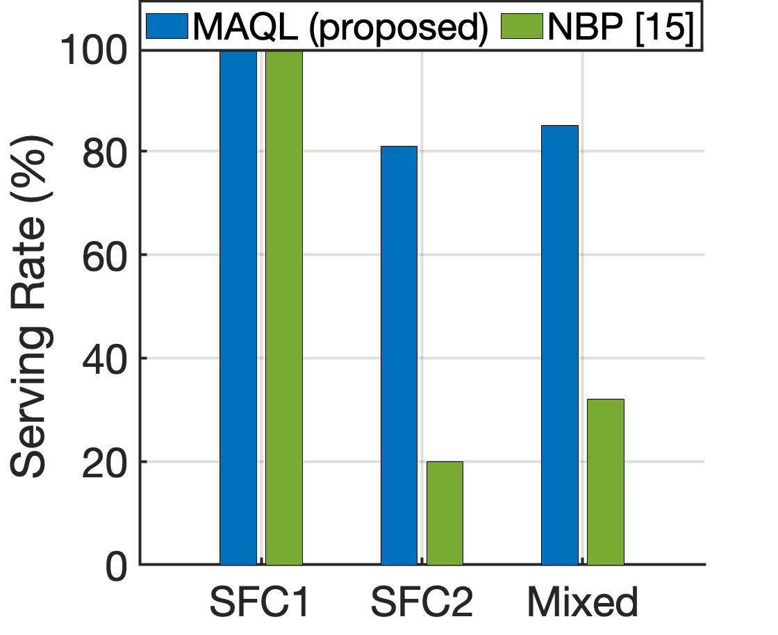
The results in terms of achieved serving rate are presented in Fig. 10; “SFC 1” stands for the case when SFC 1 is the only available service. Here, the BO-based caching results in for both the MAQL and NBP methods, which can be straightforwardly confirmed as the optimal caching strategy as SFC 1 comprises only VNF 2 and 3. In this case, every request can be handled by satellites individually, hence, both methods serve of requests. Similarly, “SFC 2” stands for the case where SFC 2 is the only available service and “Mixed” when both SFCs are available and either is requested with equal probability of . In these cases we observe that the proposed method prevails due to the limitation of NBP which considers only satellites with currently active ISLs. The superiority of exploiting the periodic movements of satellites to perform the placement using the entire LSN in the case of the proposed MAQL-based solution is evident.
4) VNF caching with large-scale service request: In this simulation, we examine the impact of cache size in a large-scale service request setting. We consider the same simulation setup described in Subsection VI-A-3 where a total of SFCs can be requested. We make the following modifications in the setup: satellites that form three subgroups with four satellites in each one and for satellites and belonging in different subgroups. To the best of our knowledge, none of the existing works in the literature have proposed a practical distribution for the popularity of VNFs. Therefore, to demonstrate the impact of the VNF popularity imbalance on the caching performance, we assume that the popularity of VNFs, i.e., , follows Zipf distribution [28]. This choice is based on Zipf’s skewness factor, , which effectively models varying levels of popularity imbalance. Particularly, we consider low and high popularity imbalance levels defined by and , respectively. The requested SFCs are generated through Algorithm 3.
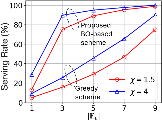
The results are illustrated in Fig. 11 where both methods achieve improved performance as the caching capacity , , increases. We compare the proposed BO-based scheme against a Greedy Caching scheme, where the popularity of VNFs is known and VNFs are cached in the descending order of their popularity. Since satellites operate independently and are not aware of the cached VNF subsets of each other, the greedy scheme, with a lack of diversity in its caching decisions, results in the same cache placement for every satellite. The presented framework can effectively capture the popularity and diversity aspects of VNFs for an effective caching strategy, as demonstrated in Fig. 11. Besides that, the bias of VNF popularity is also shown to have a significant impact with both schemes performing better when the bias defined by increases from to .
VII Conclusion
In this work, we have tackled the SFC placement problem in LSNs, aiming at optimizing long-term system performance. We have first developed an optimal offline service placement policy using a DP equation, but its high computational complexity, extensive statistical information, and centralized nature presented challenges for online use. To overcome these, we have proposed a cooperative MAQL-based approach with a parameter-sharing mechanism to manage the non-stationary satellite environment. Additionally, recognizing the dependence of SFC deployment on the pre-installed/cached VNFs on each satellite, we have incorporated a BO-based VNF caching scheme to maximize the request serving rate, where an acquisition function has guided the search towards potentially optimal caching strategies. Simulations have demonstrated that our proposed framework outperforms the most recent approaches introduced in the literature. Future work will focus on scaling the framework to handle multiple requests and exploring a distributed approach to enhance the BO-based method, particularly for applications in LEO satellite mega-constructions.
References
- [1] H. Lee, B. Lee, H. Yang, J. Kim, S. Kim, W. Shin, B. Shim, and H. V. Poor, “Towards 6G Hyper-Connectivity: Vision, Challenges, and Key Enabling Technologies,” J. Commn. Net., vol. 25, no. 3, pp. 344–354, 2023.
- [2] C. Han, X. Li, H. Ji, and H. Zhang, “Adaptive Online Service Function Chain Deployment in Large-scale LEO Satellite Networks,” in Proc. IEEE Int. Symp. Pers., Indoor, Mobile Radio Commun., Toronto, ON, Canada, 2023, pp. 1–6.
- [3] X. Qin, T. Ma, Z. Tang, X. Zhang, H. Zhou, and L. Zhao, “Service-Aware Resource Orchestration in Ultra-Dense LEO Satellite-Terrestrial Integrated 6G: A Service Function Chain Approach,” IEEE Trans. Wirel. Commun., vol. 22, no. 9, 2023.
- [4] J. He, N. Cheng, Z. Yin, H. Zhou, W. Xu, H. Peng, C. Zhou, and R. Zhang, “Service-Oriented Resource Allocation in SDN Enabled LEO Satellite Networks,” in Proc. IEEE Int. Symp. Pers., Indoor, Mobile Radio Commun., Toronto, ON, Canada, 2023, pp. 1–6.
- [5] T. Li, H. Zhou, H. Luo, Q. Xu, S. Hua, and B. Feng, “Service Function Chain in Small Satellite-Based Software Defined Satellite Networks,” China Commun., vol. 15, no. 3, pp. 157–167, 2018.
- [6] A. Leivadeas, G. Kesidis, M. Ibnkahla, and I. Lambadaris, “VNF Placement Optimization at the Edge and Cloud,” Future Internet, vol. 11, no. 3, p. 69, 2019.
- [7] G. L. Santos et al., “Service Function Chain Placement in Distributed Scenarios: A Systematic Review,” J. Netw. Syst. Manag., vol. 30, no. 1, p. 4, 2022.
- [8] K. Doan, M. Avgeris, A. Leivadeas, I. Lambadaris, and W. Shin, “Service Function Chaining in LEO Satellite Networks via Multi-Agent Reinforcement Learning,” in Proc. IEEE Global Telecommun. Conf., Kuala Lumpur, Malaysia, 2023, pp. 7145–7150.
- [9] L. Jin, L. Wang, X. Jin, J. Zhu, K. Duan, and Z. Li, “Research on the Application of LEO Satellite in IOT,” in Proc. Int. Conf. Eng. Technol. Innov., India, 2022, pp. 739–741.
- [10] A. Mokhtar and M. Azizoglu, “On the Downlink Throughput of a Broadband LEO Satellite Network with Hopping Beams,” IEEE Commun. Lett., vol. 4, no. 12, pp. 390–393, 2000.
- [11] R. Deng, B. Di, H. Zhang, L. Kuang, and L. Song, “Ultra-Dense LEO Satellite Constellations: How Many LEO Satellites Do We Need?” IEEE Trans. Wirel. Commun., vol. 20, no. 8, pp. 4843–4857, 2021.
- [12] R. Deng, B. Di, and L. Song, “Ultra-Dense LEO Satellite Based Formation Flying,” IEEE Trans. Commun., vol. 69, no. 5, pp. 3091–3105, 2021.
- [13] P. Wang, B. Di, and L. Song, “Multi-layer LEO Satellite Constellation Design for Seamless Global Coverage,” in Proc. IEEE Global Telecommun. Conf., Spain, 2021, pp. 01–06.
- [14] B. Ko and S. Kwak, “Survey of Computer Vision-Based Natural Disaster Warning Systems,” Opt. Eng., vol. 51, pp. 901–936, 2012.
- [15] X. Gao, R. Liu, A. Kaushik, J. Thompson, H. Zhang, and Y. Ma, “Dynamic Resource Management for Neighbor-Based VNF Placement in Decentralized Satellite Networks,” in Proc. Int. Conf. 6G Netw., Paris, France, 2022, pp. 1–5.
- [16] X. Gao, R. Liu, and A. Kaushik, “Virtual Network Function Placement in Satellite Edge Computing With a Potential Game Approach,” IEEE Trans. Netw. Service Manag., vol. 19, no. 2, pp. 1243–1259, 2022.
- [17] X. Qin, T. Ma, Z. Tang, X. Zhang, X. Liu, and H. Zhou, “SFC Enabled Data Delivery for Ultra-Dense LEO Satellite-Terrestrial Integrated Network,” in Proc. IEEE Global Telecommun. Conf., Rio de Janeiro, Brazil, 2022, pp. 668–673.
- [18] Z. Jia, M. Sheng, J. Li, D. Zhou, and Z. Han, “VNF-Based Service Provision in Software Defined LEO Satellite Networks,” IEEE Trans. Wirel. Commun., vol. 20, no. 9, pp. 6139–6153, 2021.
- [19] Z. Jia et al., “Joint Optimization of VNF Deployment and Routing in Software Defined Satellite Networks,” in Proc. IEEE Veh. Technol. Conf., Porto, Portugal, 2018, pp. 1–5.
- [20] Y. Cai, Y. Wang, X. Zhong, W. Li, X. Qiu, and S. Guo, “An Approach to Deploy Service Function Chains in Satellite Networks,” in Proc. IEEE/IFIP Netw. Oper. Manage. Symp., Taipei, Taiwan, 2018, pp. 1–7.
- [21] Q. Xia, G. Wang, Z. Xu, W. Liang, and Z. Xu, “Efficient Algorithms for Service Chaining in NFV-Enabled Satellite Edge Networks,” IEEE Trans. Mob. Comput., pp. 1–17, 2023.
- [22] R. Garnett, Bayesian Optimization. Cambridge Univ. Press, 2023.
- [23] L. Wasserman, All of statistics : A Concise Course in Statistical Inference. New York: Springer, 2010.
- [24] S. Pandey, J. W.-K. Hong, and J.-H. Yoo, “Q-Learning Based SFC Deployment on Edge Computing Environment,” in Proc. Asia-Parcific Netw. Oper. Manage. Symp., Daegu, Korea, 2020, pp. 220–226.
- [25] J. Liu, Y. Li, Y. Zhang, L. Su, and D. Jin, “Improve Service Chaining Performance with Optimized Middlebox Placement,” IEEE Trans. Serv. Comput., vol. 10, no. 4, pp. 560–573, 2017.
- [26] S. J. Wright and B. Recht, Coordinate Descent. Cambridge Univ. Press, 2022, p. 100–117.
- [27] C. Bogani, M. Gasparo, and A. Papini, “Generalized Pattern Search Methods for a Class of Nonsmooth Optimization Problems with Structure,” J. Comput. Appl. Math., vol. 229, no. 1, pp. 283–293, 2009.
- [28] A. Saichev, Y. Malevergne, and D. Sornette, Theory of Zipf’s Law and Beyond. Springer Berlin Heidelberg, 2009.