Core-satellite Graphs: Clustering, Assortativity and Spectral Properties

Ernesto Estrada²²2Department of Mathematics & Statistics, University of Strathclyde, 26 Richmond Street, Glasgow G1 1HX, UK (ernesto.estrada@strath.ac.uk). Michele Benzi³³3Department of Mathematics and Computer Science, Emory University, Atlanta, Georgia 30322, USA (benzi@mathcs.emory.edu).

Abstract

Core-satellite graphs (sometimes referred to as generalized friendship graphs) are an interesting class of graphs that generalize many well known types of graphs. In this paper we show that two popular clustering measures, the average Watts-Strogatz clustering coefficient and the transitivity index, diverge when the graph size increases. We also show that these graphs are disassortative. In addition, we completely describe the spectrum of the adjacency and Laplacian matrices associated with core-satellite graphs. Finally, we introduce the class of generalized core-satellite graphs and analyze their clustering, assortativity, and spectral properties.

1 Introduction

The availability of data about large real-world networked systems—commonly known as complex networks—has demanded the development of several graph-theoretic and algebraic methods to study the structure and dynamical properties of such usually giant graphs [1, 2, 3]. In a seminal paper, Watts and Strogatz [4] introduced one of such graph-theoretic indices to characterize the transitivity of relations in complex networks. The so-called clustering coefficient represents the ratio of the number of triangles in which the corresponding node takes place to the the number of potential triangles involving that node (see further for a formal definition). The clustering coefficient of a node is bounded between zero and one, with values close to zero indicating that the relative number of transitive relations involving that node is low. On the other hand, a clustering coefficient close to one indicates that this node is involved in as many transitive relations as possible. When studying complex real-world networks it is very common to report the average Watts-Strogatz (WS) clustering coefficient $\bar{C}$ as a characterization of how globally clustered a network is [1, 2]. Such idea, however, was not new as reflected by the fact that Luce and Perry [5] had proposed 50 years earlier an index to account for the network transitivity, given by the total number of triangles in the graph divided by the total number of triads existing in the graph. Such index, hereafter called the graph transitivity $C$ , was then rediscovered by Newman [6] in the context of complex networks. Here again this index is bounded between zero and one, with small values indicating poor transitivity and values close to one indicating a large one (see also [7]).

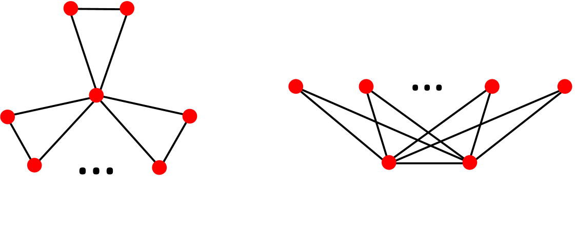
It was first noticed by Bollobás [8] and then by Estrada [1] that there are certain graphs for which the two clustering coefficients diverge. That is, there are classes of graphs for which the WS average clustering coefficient tends to one while the graph transitivity tends to zero as the size of the graphs grows to infinity. The two families indentified by Bollobás [8] and by Estrada [1] are illustrated in Figure 1 and they correspond to the so-called friendship (or Dutch windmill or $n$ -fan) graphs [9] and agave graphs [10], respectively. The friendship graphs are formed by glueing together $\eta$ copies of a triangle in a common vertex. The agave graphs are formed by connecting $s$ disjoint nodes to both nodes of a complete graph $K_{2}$ .

The friendship graphs are members of a larger family of graphs known as the windmill graphs [11, 12, 13, 14, 15]. A windmill graph $W\left(\eta,s\right)$ consists of $\eta$ copies of the complete graph $K_{s}$ [11] with every node connected to a common one (see Figure 3). In a recent paper Estrada [16] has proved that the divergence of the two clustering coefficient indices also takes place for windmill graphs when the number of nodes tends to infinity. The agave graphs belong to the general class of complete split graphs, which are the graphs consisting of a central clique and a disjoint set of nodes which are connected to all the nodes of the clique [17].

Refer to caption — Figure 1: Examples of graphs for which the average WS clustering coefficient and the graph transitivity diverge as the size of the graphs goes to infinity.

It is important to note that this divergence between the two clustering coefficients also takes place in certain real-world networks [16]. This phenomenon has passed inadverted among the plethora of papers that deals with clustering in real-world networks. In Table 1 we illustrate some results collected from the literature in which the divergence of the two clustering coefficients is observed. The dataset is selected to intentionally display the heterogeneity of classes of real-world networks which display such phenomenon. They correspond to the interchange of emails among the employees of the ENRON corporation, a CAIDA version of the Internet as Autonomous System, a metabolic network, a social network of Hollywood actors and a network of coauthors in Biology.

	$n$	$m$	$\bar{C}$	$C$
E-mail	36 692	183 831	0.50	0.09
Internet	26 475	106 762	0.21	0.007
metabolic	765	3 686	0.67	0.09
Actors	449 913	25 516 482	0.78	0.20
Coauthors	1 520 251	11 803 064	0.60	0.09

Table 1: Some real-world networks collected from the literature displaying divergence of the average WS clustering coefficient and the graph transitivity. Here

n

and

m

denote the number of nodes and edges in the various graphs.

In this work we study a class of graphs which accounts for the clustering divergence phenomenon in networks with degree disassortativity. These graphs, which we call core-satellite graphs, are formed by a central clique (the core) connected to several other cliques (the satellites) in such a way that they generalize both the complete split and the windmill graphs. We prove here that the clustering coefficients of these graphs diverge and that they are always disassortative. We also characterize completely the eigenstructure of the adjacency and the Laplacian matrices of these graphs, and comment on the asymptotic behavior of such quantities as the infection threshold and synchronizability index of these graphs. Finally, we provide evidence that supports the idea of using the core-satellite graphs as models of certain classes of real-world networks.

2 Preliminaries

Here we always consider simple undirected and connected graphs $G=(V,E)$ formed by a set of $n$ nodes (vertices) $V$ and a set of $m$ edges $E=\{(u,v)\,|\,u,v\in V\}$ between the nodes. Let us now recall an important graph operation which will be helpful in this work.

Definition 1.

The join (or complete product) $G_{1}\nabla G_{2}$ of graphs $G_{1}$ and $G_{2}$ is the graph obtained from $G_{1}\cup G_{2}$ by joining every vertex of $G_{1}$ with every vertex of $G_{2}$ .

Let us now define some specific classes of graphs which will be considered in this work. As usual, we denote with $\bar{G}$ the complement of a graph $G$ .

Definition 2.

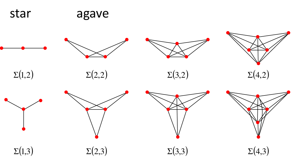
The complete split graph is $\Sigma\left(a,b\right)\cong K_{a}\nabla\bar{K}_{b}$ . The special cases $\Sigma\left(1,b\right)\cong K_{2}\nabla\bar{K}_{b}$ and $\Sigma\left(2,b\right)\cong K_{2}\nabla\bar{K}_{b}$ are known as the star and agave graphs, respectively.

In Figure 2 we show some examples of complete split graphs.

Definition 3.

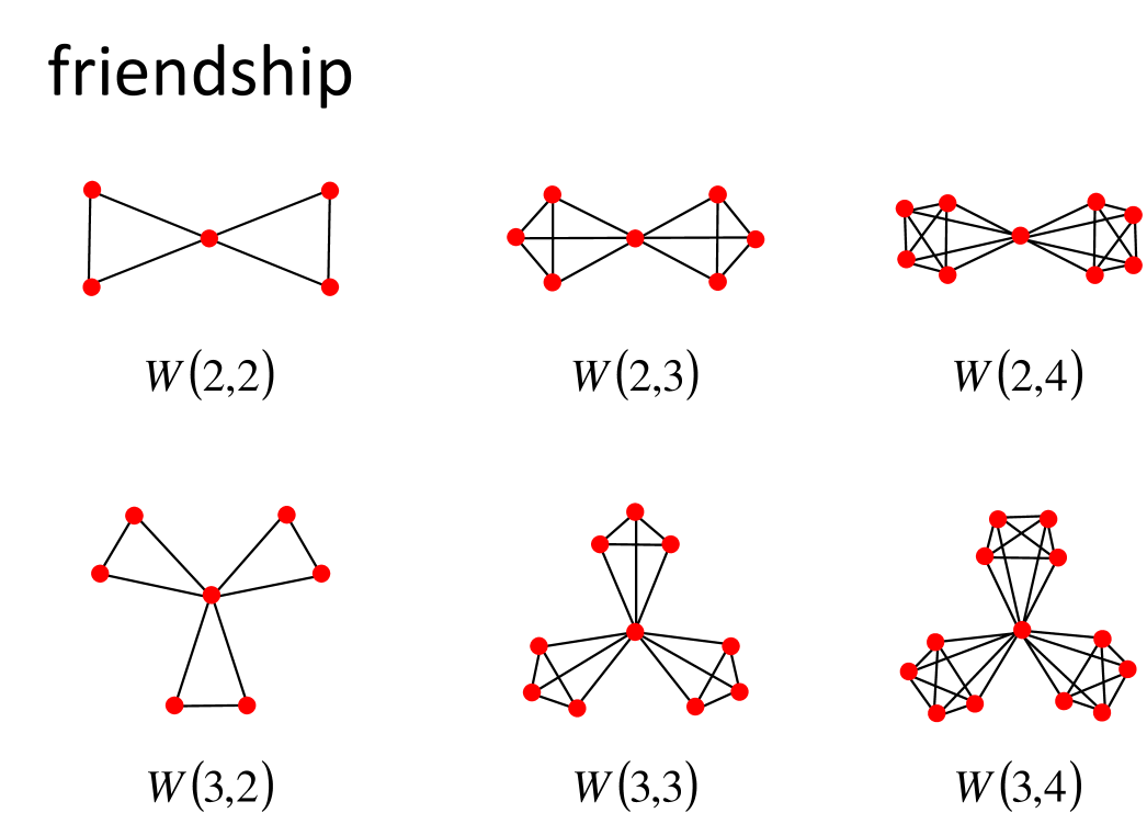
The windmill graph is $W\left(\eta,a\right)\cong K_{1}\nabla\left(\eta K_{a}\right)$ . These are the graphs consisting of $\eta$ copies of $K_{a}$ meeting in a common vertex. The special cases $W\left(\eta,2\right)\cong K_{1}\nabla\left(\eta K_{2}\right)$ are known as the friendship graphs.

In Figure 3 we show some examples of windmill graphs.

Let us now define a few graph-theoretic invariants that will be studied in this work. The so-called Watts-Strogatz clustering coefficient of a node $i$ , which quantifies the degree of transitivity of local relations in a graph is defined as [4]:

C_{i}=\frac{2t_{i}}{k_{i}(k_{i}-1)}

(1)

where $t_{i}$ is the the number of triangles in which the node $i$ participates. Taking the mean of these values as $i$ varies among all the nodes in $G$ , one gets the average WS clustering coefficient of the network $G$ :

\overline{C}=\frac{1}{n}\sum_{u=1}^{n}C_{u}.

(2)

The so-called graph transitivity is defined as [6, 7]

C=\frac{3t}{P_{2}},

(3)

where $t$ is the total number of triangles and $P_{2}=\sum_{i=1}^{n}k_{i}(k_{i}-1)/2$ .

Another important network parameter is the degree assortativity coefficient which measures the tendency of high degree nodes to be connected to other high degree nodes (assortativity) or to low degree ones (disassortativity). The assortativity coefficient is mathematically expressed as [24]:

r=\dfrac{m^{-1}\sum_{i,j\in E}k_{i}k_{j}-\dfrac{1}{4m^{2}}\left(\sum_{i,j\in E}k_{i}+k_{j}\right)^{2}}{\dfrac{1}{2m}\left(\sum_{i,j\in E}k_{i}^{2}+k_{j}^{2}\right)-\dfrac{1}{4m^{2}}\left(\sum_{i,j\in E}k_{i}+k_{j}\right)^{2}}.

(4)

Let $A=\left(a_{uv}\right)_{n\times n}$ be the adjacency matrix of the graph. We denote by $\lambda_{1}>\lambda_{2}\geq\cdots\geq\lambda_{n}$ the eigenvalues of $A$ . The dominant eigenvalue $\lambda_{1}$ is also referred to as the Perron eigenvalue or spectral radius of $A$ , denoted $\rho(A)$ . Let $\varDelta$ be the diagonal matrix of the vertex degrees of the graph. Then, the Laplacian matrix of the graph is defined by $L=\varDelta-A$ . We denote by $\mu_{1}\geq\mu_{2}\geq\cdots\geq\mu_{n-1}>\mu_{n}=0$ the eigenvalues of $L$ . The eigenvalue $\mu_{n-1}$ is known as the algebraic connectivity of the graph and the eigenvector associated to it is known as the Fiedler vector [26]. For reviews about spectral properties of graphs the reader is directed to the classic works [27, 28].

3 Core-satellite graphs

The main paradigm for defining the core-satellite graphs is the following. We consider a group of central nodes in a network which are connected among them. Then, there are a few cliques of the same size which are connected to the central core but which are not connected among them. Formally, the core-satellite graphs are defined below.

Definition 4.

Let $c\geq 1$ , $s\geq 1$ and $\eta\geq 2$ . The core-satellite graph is $\Theta\left(c,s,\eta\right)\cong K_{c}\nabla\left(\eta K_{s}\right)$ . That is, they are the graphs consisting of $\eta$ copies of $K_{s}$ (the satellites) meeting in a common clique $K_{c}$ (the core), see Fig. 4.

Remark 5.

The core-satellite graph generalizes the following classes of graphs:

•

star graphs: $\Theta\left(1,1,\eta\right)$ ;
•

agave graphs: $\Theta\left(2,1,\eta\right)$ ;
•

complete split graphs: $\Theta\left(c,1,\eta\right)$ ;
•

friendship graphs: $\Theta\left(1,2,\eta\right)$ ;
•

windmill graphs: $\Theta\left(1,s,\eta\right)$ .

The core-satellite graphs were previously defined in the literature in the context of extremal graph theory. They are named generalized friendship graphs in the works of Erdős et al. [18], Chen et al. [19] and Faudree et al. [20]. However, the same name appears in connection to at least another class of graphs. The generalized friendship graph is defined by Ahmad et al. [21], Arumugan and Nalliah [22], Shi et al. [23] and by Jahari and Alikhani [25] as the graph consisting of $r$ cycles of orders $n_{1}\geq n_{2}\geq\cdots\geq n_{r}$ having a common vertex. These graphs are also known as flowers. Thus, to avoid any confusion we propose here the more intuitive name of core-satellite for these graphs.

4 General properties of core-satellite graphs

Let $\Theta\left(c,s,\eta\right)$ be a core-satellite graph and let us designate any node in the core as $i$ and any node in a satellite as $j$ . Then, $k_{i}=c+\eta s-1$ and $k_{j}=c+s-1$ , also $n=c+\eta s$ and $m=\left(\begin{array}[]{c}c+p\\ 2\end{array}\right)-\left(\eta-1\right)\left(\begin{array}[]{c}c\\ 2\end{array}\right)$ . We now state our first result.

Theorem 6.

Let $\Theta\left(c,s,\eta\right)$ be a core-satellite graph. Then, for given values of $c$ and $s$ the average Watts-Strogatz and the transitivity coefficients diverge when the number of cliques $\eta$ tends to infinity:

\underset{\eta\rightarrow\infty}{\lim}\bar{C}=1,

(5)

\underset{\eta\rightarrow\infty}{\lim}C=0.

(6)

Proof.

First, we obtain an expression for the Watts-Strogatz clustering coefficient of windmill graphs. The Watts-Strogatz clustering coefficient of any node in the core clique of $\Theta\left(c,s,\eta\right)$ is

C_{i}=\dfrac{\eta\left(c+s-1\right)\left(c+s-2\right)-\left(c-1\right)\left(c-2\right)\left(\eta-1\right)}{\left(\eta s+c-1\right)\left(\eta s+c-2\right)},

(7)

and the rest of the nodes have $C_{j}=1$ . Thus, $\bar{C}=\left(cC_{i}+\eta s\right)/n$ , which gives

\bar{C}=1-\dfrac{cs^{2}\eta^{2}}{n\left(n-1\right)\left(n-2\right)}=1-\dfrac{c\left(n-c\right)^{2}}{n\left(n-1\right)\left(n-2\right)}

(8)

Now we consider the transitivity index of a windmill graph $\Theta\left(c,s,\eta\right)$ . The total number of triangles in $W\left(\eta,\kappa\right)$ is

t=\eta\left(\begin{array}[]{c}c+s\\ 3\end{array}\right)+\left(\eta-1\right)\left(\begin{array}[]{c}c\\ 3\end{array}\right),

(9)

and the number of 2-paths is

P_{2}=c\left(\begin{array}[]{c}n-1\\ 2\end{array}\right)+\eta s\left(\begin{array}[]{c}c+s\\ 2\end{array}\right).

(10)

Thus, after substitution we get

C=\dfrac{\eta\left(c+s\right)\left(c+s-1\right)\left(c+s-2\right)-c\left(\eta-1\right)\left(c-1\right)\left(c-2\right)}{\eta s\left(c+s-1\right)\left(c+s-2\right)+c\left(c+\eta s-1\right)\left(c+\eta s-2\right)}.

(11)

Obviously, $\underset{\eta\rightarrow\infty}{\lim}\bar{C}=1$ and $\underset{\eta\rightarrow\infty}{\lim}C=0$ for any given values of $c$ and $s$ , which proves the result. ∎

Next, we prove a result related to the way in wich nodes connect to each other in core-satellite graphs.

Theorem 7.

Let $\Theta\left(c,s,\eta\right)$ be a core-satellite graph. Then, for any values of $c\geq 1$ , $s\geq 1$ , and $\eta\geq 2$ the core-satellite graphs are disassortative, i.e., $r<0.$

Proof.

We first need a result previously obtained by Estrada [29] that expresses the assortativity coefficient in terms of subgraphs of the corresponding graph,

r=\dfrac{P_{2}\left(P_{3/2}+C-P_{2/1}\right)}{3S_{1,3}-P_{2}\left(P_{2/1}-1\right)},

(12)

where $P_{s/t}$ represents the ratio of paths of length $s$ to paths of length $t$ , $S_{1,3}$ is the number of star subgraphs with a central node and 3 pendant nodes, and $C$ is the transitivity index. It has been previously proved in [29] that the denominator of (12) is positive. Thus, the sign of the assortativity coefficient depends on the sign of $P_{3/2}+C-P_{2/1}$ . It is straighforward to realize that in a core-satellite graph the number of paths of length 3 is zero. Consequently, the sign of $r$ depends only on the sign of $C-P_{2/1}$ . We remind that $0\leq C\leq 1$ . Thus, let us consider the difference $P_{2}-P_{1}$

P_{2}-P_{1}=\dfrac{ck_{i}}{2}\left(k_{i}-1\right)+\dfrac{\eta sk_{j}}{2}\left(k_{j}-2\right).

(13)

Because $\eta\geq 2$ then $k_{i}\geq 2$ (notice that if $k_{i}=1$ the resulting graph is just $K_{2})$ . If $k_{j}=1$ the core-satellite graph corresponds to the star graph, which is a tree, and consequently has $C=0$ . Thus, the graph is diassortative. Let $k_{j}\geq 2$ , then because $\eta\geq 2$ we have that $k_{i}\geq 4$ , which implies that $P_{2}-P_{1}>1$ , i.e., $P_{2/1}>1$ and consequently $r<0$ , which proves the result. ∎

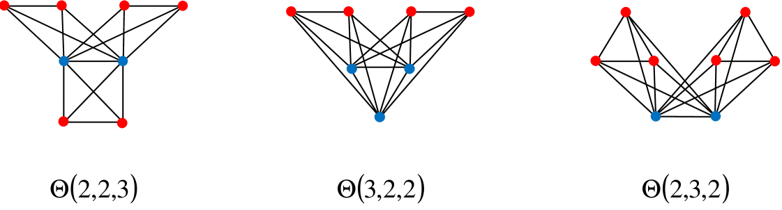
5 Spectral properties of core-satellite graphs

In this section we give a full description of the spectral properties (eigenvalues and eigenvectors) of core-satellite graphs, and we investigate extensions to more general types of graphs. We begin by proving the following result.

Theorem 8.

The spectrum of the core-satellite graph $\Theta(c,s,\eta)$ consists of:

1.

The eigenvalue $\lambda=-1$ with multiplicity $c+\eta(s-1)-1$ ;
2.

The eigenvalue $\lambda=s-1$ with multiplicity $\eta-1$ ;
3.

The eigenvalues $\lambda_{\pm}$ given by the roots of the quadratic equation

$\lambda^{2}-(c+s-2)\lambda+(c-1)(s-1)-\eta cs=0.$ (14)

Proof.

For any positive integer $p$ , we use ${\bf 1}_{p}$ to denote the column vector with all entries equal to 1. Let $A(K_{c})$ and $A(K_{s})$ denote, respectively, the adjacency matrices of the complete graphs with $c$ and $s$ nodes. Note that $A(K_{c})={\bf 1}_{c}{\bf 1}_{c}^{T}-I_{c}$ , $A(K_{s})={\bf 1}_{s}{\bf 1}_{s}^{T}-I_{s}$ with $I_{c}$ and $I_{s}$ standing for the $c\times c$ and $s\times s$ identity matrices. With an obvious ordering of the nodes, the adjacency matrix of $\Theta(c,s,\eta)$ can be written as the block matrix

A=\left[\begin{array}[]{c|ccc}A(K_{c})&{\bf 1}_{c}{\bf 1}_{s}^{T}&\cdots&{\bf 1}_{c}{\bf 1}_{s}^{T}\\[2.0pt] \hline\cr\\[-8.0pt] {\bf 1}_{s}{\bf 1}_{c}^{T}&A(K_{s})\\ \vdots&&\ddots\\[2.0pt] {\bf 1}_{s}{\bf 1}_{c}^{T}&&&A(K_{s})\end{array}\right],

(15)

with $\eta$ copies of $A(K_{s})$ appearing on the block diagonal. Now let the vector

{\bf x}=\left[\begin{array}[]{c}{\bf x}_{1}\\[2.0pt] \hline\cr\\[-8.0pt] {\bf 0}\\ \vdots\\[2.0pt] {\bf 0}\end{array}\right],\qquad{\bf x}_{1}\neq{\bf 0},

(16)

be partitioned conformally to $A$ . Then the equation $A{\bf x}=\lambda{\bf x}$ becomes

\left[\begin{array}[]{c}A(K_{c}){\bf x}_{1}\\[2.0pt] \hline\cr\\[-8.0pt] ({\bf 1}_{c}^{T}{\bf x}_{1}){\bf 1}_{s}\\ \vdots\\[2.0pt] ({\bf 1}_{c}^{T}{\bf x}_{1}){\bf 1}_{s}\end{array}\right]=\left[\begin{array}[]{c}\lambda{\bf x}_{1}\\[2.0pt] \hline\cr\\[-8.0pt] {\bf 0}\\ \vdots\\[2.0pt] {\bf 0}\end{array}\right].

Clearly, this is equivalent to $A(K_{c}){\bf x}_{1}=\lambda{\bf x}_{1}$ , and ${\bf x}_{1}\perp{\bf 1}_{c}$ . Hence, $\lambda=-1$ and there are $c-1$ linearly independent eigenvectors of the form (16). Next, consider vectors of the form

{\bf x}=\left[\begin{array}[]{c}{\bf 0}\\[2.0pt] \hline\cr\\[-8.0pt] {\bf 0}\\ \vdots\\[2.0pt] {\bf 0}\\ {\bf x}_{i}\\[2.0pt] {\bf 0}\\ \vdots\\[2.0pt] {\bf 0}\end{array}\right],\qquad{\bf x}_{i}\neq{\bf 0},\qquad i=1,\ldots,\eta,

(17)

where ${\bf x}_{i}$ corresponds to the $(i+1)$ th diagonal block of $A$ . Then the equation $A{\bf x}=\lambda{\bf x}$ becomes

\left[\begin{array}[]{c}({\bf 1}_{s}^{T}{\bf x}_{i}){\bf 1}_{c}\\[2.0pt] \hline\cr\\[-8.0pt] {\bf 0}\\ \vdots\\[2.0pt] {\bf 0}\\ A(K_{s}){\bf x}_{i}\\[2.0pt] {\bf 0}\\ \vdots\\[2.0pt] {\bf 0}\end{array}\right]=\left[\begin{array}[]{c}{\bf 0}\\[2.0pt] \hline\cr\\[-8.0pt] {\bf 0}\\ \vdots\\[2.0pt] {\bf 0}\\ \lambda{\bf x}_{i}\\[2.0pt] {\bf 0}\\ \vdots\\[2.0pt] {\bf 0}\end{array}\right].

Clearly, this is equivalent to $A(K_{s}){\bf x}_{i}=\lambda{\bf x}_{i}$ , and ${\bf x}_{i}\perp{\bf 1}_{s}$ for $i=1,\ldots,\eta$ . This yields another $\eta(s-1)$ linearly independent eigenvectors associated with the eigenvalue $\lambda=-1$ .

Now, consider vectors of the form

\left[\begin{array}[]{c}{\bf 0}\\[2.0pt] \hline\cr\\[-8.0pt] \alpha_{1}{\bf 1}_{s}\\ \vdots\\[2.0pt] \alpha_{\eta}{\bf 1}_{s}\end{array}\right],

(18)

with the $\alpha_{i}$ not all zero. Then the equation $A{\bf x}=\lambda{\bf x}$ becomes

\left[\begin{array}[]{c}\sum_{i=1}^{\eta}\alpha_{i}({\bf 1}_{s}^{T}{\bf 1}_{s}){\bf 1}_{c}\\[2.0pt] \hline\cr\\[-8.0pt] \alpha_{1}A(K_{s}){\bf 1}_{s}\\ \vdots\\[2.0pt] \alpha_{\eta}A(K_{s}){\bf 1}_{s}\end{array}\right]=\left[\begin{array}[]{c}{\bf 0}\\[2.0pt] \hline\cr\\[-8.0pt] \lambda\alpha_{1}{\bf 1}_{s}\\ \vdots\\[2.0pt] \lambda\alpha_{\eta}{\bf 1}_{s}\end{array}\right].

Since at least one of the $\alpha_{i}$ must be nonzero, this is equivalent to

A(K_{s}){\bf 1}_{s}=\lambda{\bf 1}_{s},\qquad\alpha_{1}+\cdots+\alpha_{\eta}=0.

The first of these two conditions implies that $\lambda=s-1$ , and there are exactly $\eta-1$ linearly independent eigenvectors of the form (18) since the solution space of the homogeneous linear equation $\alpha_{1}+\cdots+\alpha_{\eta}=0$ has dimension $\eta-1$ .

To determine the two remaining eigenvectors and corresponding eigenvalues, let

{\bf x}=\left[\begin{array}[]{c}{\bf 1}_{c}\\[2.0pt] \hline\cr\\[-8.0pt] \beta{\bf 1}_{s}\\ \vdots\\[2.0pt] \beta{\bf 1}_{s}\end{array}\right],\qquad\beta\neq 0.

(19)

Then the equation $A{\bf x}=\lambda{\bf x}$ becomes

\left[\begin{array}[]{c}(c-1){\bf 1}_{c}+\eta\beta s\\[2.0pt] \hline\cr\\[-8.0pt] c{\bf 1}_{s}+\beta(s-1){\bf 1}_{s}\\ \vdots\\[2.0pt] c{\bf 1}_{s}+\beta(s-1){\bf 1}_{s}\end{array}\right]=\left[\begin{array}[]{c}\lambda{\bf 1}_{c}\\[2.0pt] \hline\cr\\[-8.0pt] \lambda\beta{\bf 1}_{s}\\ \vdots\\[2.0pt] \lambda\beta{\bf 1}_{s}\end{array}\right],

which reduces to the two conditions

c-1+\eta\beta s=\lambda,\qquad c+\beta(s-1)=\lambda\beta.

(20)

Conditions (20) yield

\beta=\frac{\lambda-c+1}{\eta s},\qquad\beta=\frac{c}{\lambda-s+1}\,,

(21)

hence

\frac{\lambda-c+1}{\eta s}=\frac{c}{\lambda-s+1}

which is easily seen to become equation (14) upon multiplication of both sides by $\eta s(\lambda-s+1)$ and rearranging terms. Solving for $\lambda$ yields the two remaining (simple) eigenvalues of $A$ :

\lambda_{\pm}=\frac{1}{2}\left[c+s-2\pm\sqrt{(c-s)^{2}+4\eta cs}\,\right].

(22)

These two roots yield two distinct values $\beta_{\pm}$ of $\beta$ via (21) and thus two distinct eigenvectors of $A$ of the form (19). It is obvious that these two eigenvectors are linearly independent (indeed, mutually orthogonal). ∎

Remark 9.

This theorem generalizes the spectral analysis of windmill graphs given in [16] to core-satellite graphs.

Remark 10.

We emphasize that the proof of the previous theorem explicitly reveals the structure of the eigenvectors of $A$ ; see equations (16), (17), (18) and (19), together with the fact that the eigenvectors associated with the complete graphs are known.

We also point out another consequence of Theorem 8.

Theorem 11.

The two eigenvalues under item 3 in Theorem 8 are the extreme eigenvalues of $A$ . In particular, the Perron eigenvalue (spectral radius) $\rho(A)$ of $A$ is given by

\lambda_{+}=\frac{1}{2}\left[c+s-2+\sqrt{(c-s)^{2}+4\eta cs}\,\right]\,,

while the leftmost eigenvalue of $A$ is given by

\lambda_{-}=\frac{1}{2}\left[c+s-2-\sqrt{(c-s)^{2}+4\eta cs}\,\right]\,.

Moreover, $\lambda_{-}$ is strictly less than the other eigenvalues of $A$ .

Proof.

We have

\lambda_{+}=\frac{c+s-2+\sqrt{(c-s)^{2}+4\eta cs}}{2}>\frac{c+s-2+\sqrt{(c-s)^{2}+4cs}}{2}=\frac{c+s-2}{2}+\frac{\sqrt{(c+s)^{2}}}{2}=\frac{c+s}{2}-1+\frac{c+s}{2}=c+s-1>s-1\,,

proving that $\lambda_{+}$ exceeds the other eigenvalues of $A$ in magnitude.

Similarly,

\lambda_{-}=\frac{c+s-2-\sqrt{(c-s)^{2}+4\eta cs}}{2}<\frac{c+s-2}{2}-\frac{\sqrt{(c-s)^{2}+4cs}}{2}=\frac{c+s}{2}-1-\frac{\sqrt{(c+s)^{2}}}{2}=-1\,,

proving that $\lambda_{-}$ is strictly less than all the other eigenvalues. ∎

Remark 12.

It follows that the principal eigenvector of $A$ is of the form (19). Since this eigenvector is constant on each of the cliques forming $\Theta(c,s,\eta)$ , the eigenvector centrality [1] of each node is the same for all the nodes in each clique, as one would expect. Furthermore, for $\eta>1$ the nodes in the centrale core have higher centrality than the nodes in the satellite cliques, which is also to be expected. In other words, in (19) we have that $0<\beta<1$ . This can be shown using conditions (21) together with the computed expressions for $\lambda_{\pm}$ . See also Remark 18 below.

Remark 13.

It also follows that $\Theta(c,s,\eta)$ has exactly four distinct eigenvalues. Moreover, it is clear from the expression given for $\lambda_{+}$ that it must go to infinity as the graph size $n=c+\eta s$ goes to infinity, i.e., if at least one of the parameters $c$ , $s$ , or $\eta$ tends to infinity. It follows that the infection threshold, defined as $\tau=1/\rho(A)$ , vanishes as the graph size grows, showing that core-satellite graphs of even modest size offer almost no resistance to the spreading of infections, gossip, rumors, etc. This is of course not surprising since the diameter of a core-satellite graph is only 2. We refer to [30] for additional discussion of infection spreading in networks. See also [16] for a discussion of the special case of windmill graphs.

6 Generalizing core-satellite graphs

A more realistic scenario for modeling real-world complex networks is to consider graphs in which not all satellite cliques are identical. Consequently, we consider the generalization of core-satellite graphs to the case where the satellites cliques are not restricted to have all the same number of nodes.

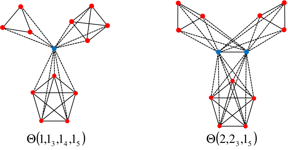
To this end, let $t\geq 1$ and consider a graph consisting of a core clique with $c$ nodes and $\eta=\eta_{1}+\eta_{2}+\cdots+\eta_{t}$ satellite cliques where $\eta_{1}$ cliques have $s_{1}$ nodes, $\eta_{2}$ cliques have $s_{2}$ nodes, … , and $\eta_{t}$ cliques have $s_{t}$ nodes, where $s_{i}\neq s_{j}$ for $i\neq j$ . Here $s_{i}\geq 1$ and $\eta_{i}\geq 1$ for all $i=1,\ldots,t$ . As before, we assume that each node in every satellite clique is connected to each node in the core clique.

We introduce the following notation: letting

{\bf s}=(s_{1},s_{2},\ldots,s_{t}),\qquad{\boldsymbol{\eta}}=(\eta_{1},\eta_{2},\ldots,\eta_{t})\,,

we denote with $\Theta(c,{\bf s},{\boldsymbol{\eta}})$ the generalized core-satellite graph just decribed. Although this notation is very convenient for expressing our mathematical results, it can be very cumbersome for illustrative examples. For that last purpose we will denote the number of cliques of a given size by an integer, using a subindex for the size of the clique as illustrated in the Figure 5. Note that such a graph has $n=c+\sum_{i=1}^{t}\eta_{i}s_{i}$ nodes. Core-satellite graphs $\Theta(c,s,\eta)$ are obtained as special cases for $t=1$ . At the other end of the spectrum we have the generalized core-satellite graphs in which all the satellite cliques have a different number of nodes, corresponding to the case $t=\eta$ , $\eta_{i}=1$ for all $i=1,\ldots,t$ .

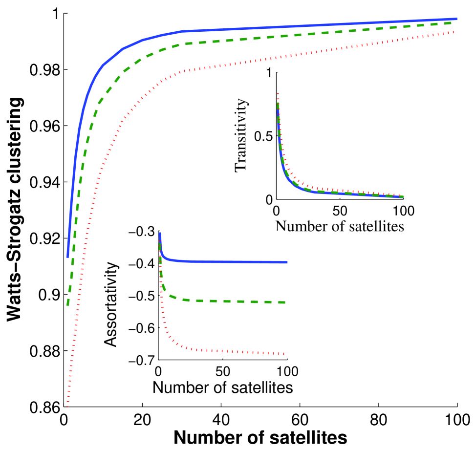
We first investigate the phenomenon of clustering divergence and the degree assortativity of these graphs. Unfortunately, it is difficult to extend the analytic approach used in section 4 to the case of generalized core-satellite graphs. Therefore, we perform numerical experiments instead. Our computations indicate that the clustering divergence phenomenon observed for the simple core-satellite graphs also occurs in the generalized case. These graphs also display degree disassortativity like their simpler analogues. In Figure 6 we illustrate the divergence of the clustering coefficients of these graphs and the increase of their disassortativity as the number of satellite cliques in the graph increases. For the sake of brevity, we only report here results for three kinds of generalized core-satellite graphs having cores with 3, 5 and 10 nodes (we remark that in real-world networks it is rare to find cliques od size larger than 10 [1]). Then, we consider satellites of size 3, 5 and 7 and generate graphs $\Theta\left(c,\left(3,5,7\right),\left(p,p,p\right)\right)$ with $c\in\left\{3,5,10\right\}$ and $1\leq p\leq 100$ . As can be seen in Fig. 6, as the number of satellites increases the average Watts-Strogatz clustering coefficient approaches the asymptotic value 1, while the transitivity index drops to zero. The increase of the Watts-Strogatz index is slower for the graphs with bigger core as expected by the fact that here more nodes with low clustering exists, namely, those in the core. However, the assortativity coefficient of these graphs decays much faster than that for graphs with smaller cores. In all cases, the assortativity coefficient is negative, similarly to what happens with the simple core-periphery graphs.

Next, we study the spectral properties of the generalized core-satellite graphs. Let us define the $c\times(\eta_{i}s_{i})$ matrices

B_{i}=\underbrace{\left[{\bf 1}_{c}{\bf 1}_{s_{i}}^{T}\,\,\,\,\,{\bf 1}_{c}{\bf 1}_{s_{i}}^{T}\,\,\,\,\,\cdots\,\,\,\,\,{\bf 1}_{c}{\bf 1}_{s_{i}}^{T}\right]}_{\eta_{i}{\rm\;times}}\,,\qquad i=1,\ldots,t\,,

and the $(\eta_{i}s_{i})\times(\eta_{i}s_{i})$ block diagonal matrices

A_{i}=\underbrace{A(K_{s_{i}})\oplus\cdots\oplus A(K_{s_{i}})}_{\eta_{i}{\rm\;times}}=\left[\begin{array}[]{cccc}A(K_{s_{i}})\\ &A(K_{s_{i}})\\ &&\ddots\\ &&&A(K_{s_{i}})\end{array}\right],\qquad i=1,\ldots,t

(with $\eta_{i}$ identical diagonal blocks). Then, for a suitable ordering of the nodes, the adjacency matrix of $\Theta(c,{\bf s},{\boldsymbol{\eta}})$ , can be written in block form as

A=\left[\begin{array}[]{c|cccc}A(K_{c})&B_{1}&B_{2}&\cdots&B_{t}\\[2.0pt] \hline\cr\\[-5.0pt] B_{1}^{T}&A_{1}\\[2.0pt] B_{2}^{T}&&A_{2}\\ \vdots&&&\ddots\\[2.0pt] B_{t}^{T}&&&&A_{t}\end{array}\right]\,.

(23)

This matrix is $n\times n$ with $n=c+\sum_{i=1}^{t}\eta_{i}s_{i}$ . We have the following generalization of Theorem 8.

Theorem 14.

The spectrum of the generalized core-satellite graph $\Theta(c,{\bf s},{\boldsymbol{\eta}})$ consists of

1.

The eigenvalue $\lambda=-1$ with multiplicity $c+\sum_{i=1}^{t}\eta_{i}(s_{i}-1)-1$ ;
2.

The eigenvalue $s_{i}-1$ with multiplicity $\eta_{i}-1$ , for all $i=1,\ldots,t$ with $\eta_{i}>1$ ;
3.

The roots of the following algebraic equation of degree $t+1$ :

$(\lambda-c+1)\prod_{i=1}^{t}(\lambda-s_{i}+1)=c\,\sum_{i=1}^{t}\eta_{i}s_{i}\prod_{j\neq i}(\lambda-s_{j}+1)\,,$ (24)

each of multiplicity one.

Proof.

It is straightforward to verify that $A$ has $c-1$ linearly independent eigenvectors of the form (16) corresponding to the eigenvalue $\lambda=-1$ . Likewise, it is easy to check that $A$ has $\sum_{i=1}^{t}(s_{i}-1)\eta_{i}$ linearly independent eigenvectors of the form (17) with $s=s_{i}$ , also corresponding to the eigenvalue $\lambda=-1$ . Hence, $A$ has (at least) $c+\sum_{i=1}^{t}\eta_{i}(s_{i}-1)-1=c+\sum_{i=1}^{t}\eta_{i}s_{i}-\eta-1$ linearly independent eigenvectors corresponding to the eigenvalue $\lambda=-1$ ; since the total number of nodes is $n=c+\sum_{i=1}^{t}\eta_{i}s_{i}$ , there remain $\eta+1=\sum_{i=1}^{t}\eta_{i}+1$ eigenvalues to account for.

Let us first assume that $\eta_{i}>1$ for some $i$ . Consider a nonzero vector of the form

{\bf x}=\left[\begin{array}[]{c}{\bf 0}\\ \hline\cr{\bf 0}\\ \vdots\\[2.0pt] {\bf 0}\\ \hline\cr\alpha_{1}{\bf 1}_{s_{i}}\\ \alpha_{2}{\bf 1}_{s_{i}}\\ \vdots\\[2.0pt] \alpha_{\eta_{i}}{\bf 1}_{s_{i}}\\ \hline\cr{\bf 0}\\ \vdots\\[2.0pt] {\bf 0}\end{array}\right]\,,\qquad\alpha_{1}+\cdots+\alpha_{\eta_{i}}=0\,,

(25)

where the (possible) nonzeros in ${\bf x}$ occur in the positions that correspond to the diagonal block $A_{i}$ in $A$ . Then one can easily check that ${\bf x}$ is eigenvector of $A$ associated to the eigenvalue $\lambda=s_{i}-1$ , and from the condition on the $\alpha_{i}$ we immediately deduce that there are $\eta_{i}-1$ linear independent vectors of the form (25).

There remain $t+1$ eigenvalues to account for, where $t$ is between $1$ and $\eta$ . When $t=1$ all the satellite cliques are identical and we are back under the assumptions of Theorem 8, hence the remaining two eigenvalues are the roots of the quadratic equation (14), to which (24) reduces for $t=1$ .

Assume $t>1$ and consider a vector of the form

{\bf x}=\left[\begin{array}[]{c}{\bf 1}_{c}\\[2.0pt] \hline\cr\\[-8.0pt] \beta_{1}{\bf 1}_{s_{1}\eta_{1}}\\ \vdots\\[2.0pt] \beta_{t}{\bf 1}_{s_{t}\eta_{t}}\end{array}\right].

(26)

We note that vectors of this form are automatically orthogonal to all eigenvectors of the form (16) (with ${\bf x}_{1}\perp{\bf 1}_{c}$ ), to all eigenvectors of the form (17) (with ${\bf x}_{i}\perp{\bf 1}_{s_{i}}$ ), and to all eigenvectors of the form (25). Also, the span ${\cal S}$ of all vectors of the form (26) has dimension $t+1$ . Hence, it must be the invariant subspace of $A$ spanned by the eigenvectors associated with the remaining $t+1$ eigenvalues of $A$ . Finally, we observe that any vector in ${\cal S}$ is also of the form (26) up to a scalar multiple.

For such vectors, the equation $A{\bf x}=\lambda{\bf x}$ becomes

\left[\begin{array}[]{c}(c-1){\bf 1}_{c}+\sum_{i=1}^{t}\beta_{i}\eta_{i}s_{i}{\bf 1}_{c}\\[2.0pt] \hline\cr\\[-8.0pt] c{\bf 1}_{s_{1}\eta_{1}}+\beta_{1}(s_{1}-1){\bf 1}_{s_{1}\eta_{1}}\\ \vdots\\[2.0pt] c{\bf 1}_{s_{t}\eta_{t}}+\beta_{t}(s_{t}-1){\bf 1}_{s_{t}\eta_{t}}\end{array}\right]=\left[\begin{array}[]{c}\lambda{\bf 1}_{c}\\[2.0pt] \hline\cr\\[-8.0pt] \lambda\beta_{1}{\bf 1}_{s_{1}\eta_{1}}\\ \vdots\\[2.0pt] \lambda\beta_{t}{\bf 1}_{s_{t}\eta_{t}}\end{array}\right].

(27)

Conditions (27) can be rewritten in the form

c-1+\sum_{i=1}^{t}\beta_{i}\eta_{i}s_{i}=\lambda\,,

(28)

together with

c+\beta_{i}(s_{i}-1)=\lambda\beta_{i}\,,\qquad i=1,\ldots,t.

(29)

Rearranging conditions (29) we obtain

\beta_{i}=\frac{c}{\lambda-s_{i}+1}\,,\qquad i=1,\ldots,t.

(30)

Substituting (30) into (28) we obtain

c-1+c\,\sum_{i=1}^{t}\frac{\eta_{i}s_{i}}{\lambda-s_{i}+1}=\lambda\,,

or, equivalently,

\sum_{i=1}^{t}\frac{\eta_{i}s_{i}}{\lambda-s_{i}+1}=\frac{\lambda-c+1}{c}\,.

The left-hand side of the last equation can be rewritten as

\frac{\sum_{i=1}^{t}\eta_{i}s_{i}\prod_{j\neq i}(\lambda-s_{j}+1)}{\prod_{i=1}^{t}(\lambda-s_{i}+1)}\,,

finally leading to the equation

(\lambda-c+1)\prod_{i=1}^{t}(\lambda-s_{i}+1)=c\sum_{i=1}^{t}\eta_{i}s_{i}\prod_{j\neq i}(\lambda-s_{j}+1)\,,

which is precisely (24). Next, we will show that the $t+1$ roots of this equation are all distinct, therefore each root $\lambda_{i}$ yields a distinct value of $\beta_{i}$ via (30) and therefore a distinct eigenvector (26), thus completing the proof. For suppose that there is a root $\bar{\lambda}$ of (24) of multiplicity at least two. Then the vector

{\bf x}=\left[\begin{array}[]{c}{\bf 1}_{c}\\[2.0pt] \hline\cr\\[-8.0pt] \bar{\beta}_{1}{\bf 1}_{s_{1}\eta_{1}}\\ \vdots\\[2.0pt] \bar{\beta}_{t}{\bf 1}_{s_{t}\eta_{t}}\end{array}\right],\qquad\bar{\beta}_{i}=\frac{c}{\bar{\lambda}-s_{i}+1}\,,\qquad i=1,\ldots,t,

is an eigenvector of $A$ associated with $\bar{\lambda}$ . But then there must be another eigenvector ${\bf y}$ of $A$ associated with the same eigenvalue $\bar{\lambda}$ and orthogonal to ${\bf x}$ . As argued above, this eigenvector ${\bf y}$ must lie in the subspace ${\cal S}$ , and therefore be again of the form (25). But when we impose ${\bf y}$ to be of the form (25) and to satisfy $A{\bf y}=\bar{\lambda}{\bf y}$ we are forced to conclude that ${\bf y}={\bf x}$ , contradicting the orthogonality requirement. Hence, all roots of (24) must be simple. In particular, when all the cliques have different size ( $\eta_{i}=1$ for all $i=1,\ldots,t$ ) there are $\eta+1$ eigenvalues given by the roots of (24), and no eigenvalues of the form $\lambda=s_{i}-1$ . This completes the proof. ∎

Remark 15.

It is well known (Abel–Ruffini Theorem) that the solution by radicals of the general algebraic equation of degree 5 or higher is impossible. We do not know if the equation (24) is solvable by radicals for any values of $s_{i}$ , $\eta_{i}$ , and $t\geq 4$ . For $t=2$ and $t=3$ equation (24) can be solved by radicals, but the roots are given by rather complicated expressions (Cardano’s and Ferrari’s formulas). Hence, we do not attempt to explicitly write down the roots of (24).

Remark 16.

The number of distinct eigenvalues of $\Theta(c,{\bf s},{\boldsymbol{\eta}})$ is given by

t+2+|\{i\,|\,\eta_{i}>1\}|\,,

where $|X|$ is the cardinality of the set $X$ . This quantity is equal to $t+2$ (or $\eta+2$ , equivalently) when all the $t$ satellite cliques have different sizes.

Theorem 17.

The spectral radius (Perron eigenvalue) $\rho(A)$ of $A$ is given by the largest root of (24) and satisfies the bounds

c-1+\max_{1\leq i\leq t}s_{i}<\rho(A)<c-1+\sum_{i=1}^{t}\eta_{i}s_{i}\,.

(31)

Proof.

We begin by recalling the well known inequalities

\min_{1\leq i\leq n}\,\sum_{j=1}^{n}a_{ij}<\rho(A)<\max_{1\leq i\leq n}\,\sum_{j=1}^{n}a_{ij},

(32)

which hold for the spectral radius of any nonnegative irreducible matrix with non-constant row sums [31, Lemma 2.5]. In our case the upper bound is the maximum degree, which is attained by each node in the core clique and is equal to $n-1=c-1+\sum_{i=1}^{t}\eta_{i}s_{i}$ . The lower bound in (32) yields $\rho(A)>c+\min_{1\leq i\leq t}s_{i}-1$ , which in general is not enough to conclude that $\rho(A)$ is given by the largest root of (24) by Theorem 14. However, we can improve on this lower bound as follows. Assume (without loss of generality) that $s_{1}=\max_{1\leq i\leq t}s_{i}$ and consider a vector of the form

{\bf x}=\left[\begin{array}[]{c}{\bf 1}_{c}\\[2.0pt] \hline\cr\\[-8.0pt] {\bf 1}_{s_{1}\eta_{1}}\\ {\bf 0}\\ \vdots\\[2.0pt] {\bf 0}\end{array}\right],

then

A{\bf x}=\left[\begin{array}[]{c}(c-1+s_{1}\eta_{1}){\bf 1}_{c}\\[2.0pt] \hline\cr\\[-8.0pt] (c-1+s_{1}){\bf 1}_{s_{1}\eta_{1}}\\ c{\bf 1}_{s_{2}\eta_{2}}\\ \vdots\\[2.0pt] c{\bf 1}_{s_{t}\eta_{t}}\end{array}\right]\geq(c-1+s_{i}){\bf x}\,,\qquad\forall i=1,\ldots,t.

Hence, we have found a nonnegative vector ${\bf x}$ such that $A{\bf x}\geq r{\bf x}$ for $r=c-1+\max_{1\leq i\leq t}s_{i}$ . By a well known result (see [32, section 3]) this implies that $\rho(A)\geq r$ . Finally, it is straightforward to check that $\lambda=c-1+s_{1}$ is not a root of (24), therefore it must be $\rho(A)>c-1+s_{1}=c-1+\max_{1\leq i\leq t}s_{i}$ , proving the lower bound in (31). ∎

Remark 18.

It follows that the principal eigenvector of $A$ is of the form (26). Since this eigenvector is constant on each of the cliques forming $\Theta(c,{\bf s},{\boldsymbol{\eta}})$ , the eigenvector centrality of each node is the same for all the nodes within a given clique, as one would expect. Furthermore, the nodes in the core clique have higher centrality than the nodes in any of the satellite cliques (assuming of course there is more than one of them), which is also to be expected. In other words, in (25) we have that $0<\beta_{i}<1$ for all $i=1,\ldots,t$ . To see this, note that the $\beta_{i}$ are given by

\beta_{i}=\frac{c}{\rho(A)-s_{i}+1}\qquad(i=1,\ldots,t),

see (30). By Theorem 17 we have $\rho(A)>c-1+s_{i}$ for all $i=1,\ldots,t$ , hence $\rho(A)-s_{i}+1>c$ and therefore $0<\beta_{i}<1$ for all $i=1,\ldots,t$ .

Theorem 19.

The spectral radius of a generalized core-satellite graph goes to infinity as the graph size $n$ goes to infinity.

Proof.

Let $\hat{A}$ be the adjacency matrix of the star graph with $n$ nodes, with the central node numbered first. The spectrum of $\hat{A}$ consists of the eigenvalue 0 of multiplicity $n-2$ , plus the eigenvalues $\pm\sqrt{n-1}$ . In particular, $\rho(\hat{A})=\sqrt{n-1}$ . If $A$ is the adjacency matrix of a generalized core-satellite graph with $n$ nodes, it is straightforward that $A\geq\hat{A}$ , where the inequality is component-wise. It is well known [33, page 520] that this implies $\rho(A)\geq\rho(\hat{A})$ , hence we conclude that the spectral radius of $A$ tends to infinity as the graph size tends to infinity. ∎

Remark 20.

This result implies that in any generalized core-satellite graph, the infection threshold $\tau$ vanishes as the graph size grows, see Remark 13. Again, since the diameter of a generalized core-satellite graph is constant and equal to 2, this is to be expected.

We conclude this section with the description of the spectrum of the graph Laplacian $L$ of $\Theta(c,{\bf s},{\boldsymbol{\eta}})$ . Letting $\gamma=\sum_{i=1}^{t}\eta_{i}s_{i}$ and

L_{i}=\underbrace{L(K_{s_{i}})\oplus\cdots\oplus L(K_{s_{i}})}_{\eta_{i}{\rm\;times}},

the graph Laplacian of $\Theta(c,{\bf s},{\boldsymbol{\eta}})$ can be written as

L=\left[\begin{array}[]{c|cccc}L(K_{c})+\gamma I_{c}&-B_{1}&-B_{2}&\cdots&-B_{t}\\[2.0pt] \hline\cr\\[-5.0pt] -B_{1}^{T}&L_{1}+cI_{\eta_{1}s_{1}}\\[2.0pt] -B_{2}^{T}&&L_{2}+cI_{\eta_{2}s_{2}}\\ \vdots&&&\ddots\\[2.0pt] -B_{t}^{T}&&&&L_{k}+cI_{\eta_{t}s_{t}}\end{array}\right]\,.

(33)

We have the following result.

Theorem 21.

The spectrum of the graph Laplacian associated with the generalized core-satellite graph $\Theta(c,{\bf s},{\boldsymbol{\eta}})$ consists of

1.

The eigenvalue $\mu=c+\sum_{i=1}^{t}\eta_{i}s_{i}=n$ with multiplicity $c$ ;
2.

The eigenvalue $\mu=c+s_{i}$ with multiplicity $\eta_{i}(s_{i}-1)$ , for $1\leq i\leq t$ ;
3.

The eigenvalue $\mu=c$ with multiplicity $\sum_{i-1}^{t}\eta_{i}-1=\eta-1$ ;
4.

The eigenvalue $\mu=0$ with multiplicity one.

Proof.

It is straightforward to verify that $L$ has $c-1$ linearly independent eigenvectors of the form (16) with ${\bf x}_{1}\perp{\bf 1}_{c}$ associated to the eigenvalue $\mu=c+\sum_{i=1}^{t}\eta_{i}s_{i}$ . In addition, the vector

{\bf x}=\left[\begin{array}[]{c}{\bf 1}_{c}\\[2.0pt] \hline\cr\\[-8.0pt] \beta{\bf 1}_{\eta_{1}s_{1}}\\ \vdots\\[2.0pt] \beta{\bf 1}_{s_{t}\eta_{t}}\end{array}\right],\qquad\beta=-\frac{c}{\sum_{i=1}^{t}\eta_{i}s_{i}}\,,

is also eigenvector of $L$ associated with the eigenvalue $\mu=c+\sum_{i=1}^{t}\eta_{i}s_{i}=n$ .

Next, it is easily checked that every nonzero vector of the form (17) with ${\bf x}_{i}\perp{\bf 1}_{s_{i}}$ is an eigenvector of $L$ associated with the eigenvalue $\mu=c+s_{i}$ , and there are exactly $\eta_{i}(s_{i}-1)$ linearly independent eigenvectors of that form.

Consider now vectors of the form

{\bf x}=\left[\begin{array}[]{c}{\bf 0}\\[2.0pt] \hline\cr\\[-8.0pt] {\bf x}_{1}\\ \vdots\\[2.0pt] {\bf x}_{t}\end{array}\right]\,,\qquad{\rm where}\qquad{\bf x}_{i}=\left[\begin{array}[]{c}\alpha_{1i}{\bf 1}_{s_{i}}\\ \alpha_{2i}{\bf 1}_{s_{i}}\\ \vdots\\[2.0pt] \alpha_{\eta_{i}i}{\bf 1}_{s_{i}}\end{array}\right]\qquad(i=1,\ldots,t).

(34)

Then the equality $L{\bf x}=\mu{\bf x}$ is satisfied for $\mu=c$ if and only if

\sum_{i=1}^{t}s_{i}\sum_{j=1}^{\eta_{i}}\alpha_{ji}=0\,.

(35)

Equation (35) is a homogeneous linear equation in the unknowns $\alpha_{ji}$ , with $1\leq i\leq t$ and $1\leq j\leq\eta_{i}$ . Since the number of unknowns is $\eta_{1}+\cdots+\eta_{t}=\eta$ , equation (35) admits $\eta-1$ linearly independent solutions, each leading to a distinct eigenvector (34) of $L$ associated with $c$ .

Finally, since $\Theta(c,{\bf s},{\boldsymbol{\eta}})$ is connected, $L$ has the simple eigenvalue zero associated with the eigenvector with constant entries. ∎

Remark 22.

The Laplacian eigenvalues of $\Theta(c,{\bf s},{\boldsymbol{\eta}})$ can also be obtained from general results about the Laplacian eigenvalues of the join of two (or more) graphs and the fact that the Laplacian eigenvalues of a complete graph with $p$ nodes are known (they are $\mu=p$ with multiplicity $p-1$ and $\mu=0$ with multiplicity 1); see, e.g., [34, Theorem 2.20]. The above proof has the advantage of being self-contained and of explicitly exhibiting the eigenvectors of $L$ .

Remark 23.

It follows from Theorem 21 that the Laplacian of a generalized core-satellite graph $\Theta(c,{\bf s},{\boldsymbol{\eta}})$ , with $t>1$ , has exactly $t+3$ distinct eigenvalues. For a core-satellite graph $\Theta(c,s,\eta)$ (where $t=1$ and $\eta_{1}=\eta>1$ ), the number of distinct eigenvalues is four: $\mu=0$ , $\mu=c$ , $\mu=c+s$ , and $\mu=c+\eta s$ (see also Remark 13).

Remark 24.

We observe that (generalized) core-satellite graphs are Laplacian-integral, i.e., the Laplacian eigenvalues are all integers. Moreover, the algebraic connectivity (smallest nonzero Laplacian eigenvalue) of a generalized core-satellite graph is equal to $c$ , the size of the core clique, and is independent of the number or size of the satellite cliques. This is to be expected, since generalized core-satellite graphs can be disconnected by disconnecting the core clique.

Remark 25.

The ratio between the smallest nonzero eigenvalue of $L$ and the largest eigenvalue of $L$ is known as the synchronization index of the network: $Q=\mu_{n-1}/\mu_{1}$ . Theorem 21 implies that

Q=\frac{c}{c+\sum_{i=1}^{t}\eta_{i}s_{i}}=\frac{c}{n}\,.

In particular, for windmill graphs we recover the fact that $Q=1/n$ , as already observed in [16]. Therefore, any two core-satellite graphs of the same size $n$ and with the same core clique $K_{c}$ have exactly the same synchronization index, a somewhat surprising result. Moreover, if $c$ is fixed and $n$ grows, the synchronization index decreases. This implies that unless the core size $c$ grows and the number and size of satellite cliques remains constant (or bounded), large (generalized) core-satellite graphs are bad synchronizers. We refer to [35, 36, 37] for detailed discussions of network synchronizability.

7 Conclusions

Real-world graphs have a great variety of structures and complexities. Hence, the existence of different mathematical models—Erdős-Rényi, Barabási-Albert, Watts-Strogatz, random geometric graphs, etc. However, not all of the structural properties of real-world graphs are captured by these models. One simple example is the local-global clustering coefficient divergence. This structural effect is simply due to the fact that in some networks the local clustering tends to the maximum while the global one tends to the minimum when the size of the graphs grows to infinity. Here we have proposed a general class of graphs for which this clustering divergence is observed and can be studied analytically. These graphs—here proposed to be called core-satellite graphs—are characterized by a central core of nodes which are connected to a few satellites which may be of the same or different sizes. In this work we have investigated some general properties of these graphs, e.g., clustering coefficients, assortativity coefficients, as well as the eigenstructure of both the adjacency and the Laplacian matrices. Core-satellite graphs can also be easily modified so as to model other properties of complex networks, such as hierarchical structure [38]. All of these make core-satellite graphs a flexible model for certain classes of real-world networks, opening some new possibilities for the analytic modeling of these systems.

Acknowledgements

EE thanks the Royal Society of London for a Wolfson Research Merit Award. MB was supported in part by National Science Foundation grant DMS-1418889.

References

[1] E. Estrada, The Structure of Complex Networks. Theory and Applications, Oxford University Press, 2011.
[2] M. E. J. Newman, The structure and function of complex networks, SIAM Rev. 45 (2003) 167–256.
[3] L. F. Costa, O. N. Oliveira Jr, G. Travieso, F. A. Rodrigues, P. R. Villas Boas, L. Antiqueira, M. P. Viana, L. E. Correa Rocha. Analyzing and modeling real-world phenomena with complex networks: a survey of applications, Adv. Phys. 60 (2011) 329–412.
[4] D. J. Watts, S. H. Strogatz, Collective dynamics of ‘small-world’ networks, Nature, 393 (1998) 440-442.
[5] R. D. Luce, A. D. Perry, A method of matrix analysis of group structure, Psychometrika 14 (1949) 95–116.
[6] M. E. J. Newman, The structure of scientific collaboration networks, Proc. Natl. Acad. Sci. USA 98 (2001) 404-409.
[7] S. Wasserman, K. Faust, Social Network Analysis, Cambridge University Press, Cambridge, 1994.
[8] B. Bollobás, Mathematical results on scale-free random graphs, in: Bornholdt, S., Schuster, H. G. (Eds.), Handbook of Graph and Networks: From the genome to the internet, Wiley-VCH, Weinheim, (2003) 1-32.
[9] P. Erdős, A. Rényi, V. Sós, On a problem of graph theory, Studia Sci. Math. Hungar. 1 (1966) 215-235.
[10] E. Estrada, E. Estrada-Vargas, Distance-sum heterogeneity in graphs and complex networks, Appl. Math. Comput. 218 (2012) 10393-10405.
[11] J. A. Gallian, A survey: recent results, conjectures, and open problems in labeling graphs, J. Graph Theor. 13 (1989) 491-504.
[12] J. F. Wang, F. Belardo, Q. X. Huang, B. Borovicanin, On the largest Q-eigenvealues of graphs, Discr. Math. 310 (2010) 2858-2866.
[13] J. F. Wang, H. Zhao, Q. Huang, Spectral characterization of multicone graphs, Czech. Math. J. 62 (2012) 117-126.
[14] K. C. Das, Proof of conjectures on adjacency eigenvalues of graphs. Discr. Math. 313 (2013) 1925.
[15] A. Abdollahi, S. Janbaz, M. R. Obudi, Graphs cospectral with a friendship graph or its complement, ArXiv:1307.5411v1 (2013).
[16] E. Estrada, When local and global clustering of networks diverges, Linear Algebra Appl., in press (2015).
[17] S. Foldes, P. L. Hammer, Split graphs, University of Waterloo, CORR 76-3, March 1976.
[18] P. Erdős, Z. Furedi, R. J. Gould, D. S. Gunderson, Extremal graphs for intersecting triangles, J. Combin. Theor. B 64 (1995) 89-100.
[19] G. Chen, R. J. Gould, F. Pfender, B. Wei, Extremal graphs for intersecting cliques, J. Combin. Theor. B 89 (2003) 159-171.
[20] R. Faudree, M. Ferrara, R. Gould, M. Jacobson, tKp-saturated graphs of minimum size, Discr. Math. 309 (2009) 5870-5876.
[21] S. Arumugam, M. Nalliah, Super (a, d)-edge antimagic total labelings of friendship graphs, Australas. J. Combin. 53 (2012) 237-243.
[22] A. Ahmad, K. M. Awan, I. Javaid, Total vertex irregularity strength of wheel related graphs, Australas. J. Combin. 51 (2011) 147-156.
[23] D. Shi, W. Li, Q. Zhang, X. Pan, Efficient Mod Sum Labeling Scheme of Generalized Friendship Graph, in: Informatics and Management Science II (pp. 3-8). Springer London (2013).
[24] M. E. J. Newman, Assortative mixing in networks, Phys. Rev. Lett. 89 (2002) 208701.
[25] S. Jahari, S. Alikhani, Domination polynomial of generalized friendship and generalized book graphs. arXiv preprint arXiv:1501.05856 (2015).
[26] M. Fiedler, Algebraic connectivity of graphs, Czech. Math. J. 23 (1973) 298-305.
[27] D. M. Cvetković, M. Doob, H. Sachs, Spectra of Graphs: Theory and Application, Academic Press, 1980.
[28] D. M. Cvetković, P. Rowlinson, and S. Simic, Eigenspaces of Graphs, Cambridge University Press, 1997.
[29] E. Estrada, Combinatorial study of degree assortativity in networks. Phys. Rev. E 84 (2011) 047101.
[30] A. Barrat, M. Barthelemy, and A. Vespignani, Dynamical Processes on Complex Networks, Cambridge University Press, 2008.
[31] R. S. Varga, Matrix Iterative Analysis, Prentice-Hall, 1962.
[32] I. Marek, D. B. Szyld, Comparison theorems for weak splittings of bounded operators, Numer. Math. 58 (1990) 387-397.
[33] R. A. Horn and C. R. Johnson, Matrix Analysis, Second Edition, Cambridge University press, 2013.
[34] R. Merris, Laplacian matrices of graphs: A survey, Linear Algebra Appl. 197/198 (1994) 143-176.
[35] G. Chen, Z. Duan, Network synchronizability analysis: A graph-theoretic approach, Chaos, 18 (2008) 037102.
[36] G. Chen, X.-F. Wang, X. Li. Fundamentals of Complex Networks: Models, Structures and Dynamics, Wiley, 2015.
[37] M. Barahona, L. M. Pecora, Synchronization in small-world systems, Phys. Rev. Lett., 89 (2002) 054101.
[38] E. Ravasz, A.-L. Barabási, Hierarchical organization in complex networks, Phys. Rev. E 67 (2003) 026112.