Correlation of the Superconducting Critical Temperature with Spin and Orbital Excitation Energies in (CaxLa1-x)(Ba1.75-xLa0.25+x)Cu3Oy as Measured by Resonant Inelastic X-ray Scattering
Abstract
Electronic spin and orbital () excitation spectra of (CaxLa1-x)(Ba1.75-xLa0.25+x)Cu3Oy samples are measured by resonant inelastic x-ray scattering (RIXS). In this compound, of samples with identical hole dopings is strongly affected by the Ca/Ba substitution due to subtle variations in the lattice constants, while crystal symmetry and disorder as measured by line-widths are independent. We examine two extreme values of and two extreme values of hole-doping content corresponding to antiferromagnetic and superconducting states. The dependence of the spin mode energies is approximately the same for both the antiferromagnetic and superconducting samples. This clearly demonstrates that RIXS is sensitive to even in doped samples. A positive correlation between the superexchange and the maximum of at optimal doping () is observed. We also measured the dependence of the and orbital splittings. We infer that the effect of the unresolved excitation on is much smaller than the effect of . There appears to be dispersion in the peak of up to 0.05 eV. Our fitting of the peaks furthermore indicates an asymmetric dispersion for the excitation. A peak at 0.8 eV is also observed, and attributed to a excitation in the chain layer.
pacs:
74.62.Bf, 74.25.Ha, 75.30.Ds, 78.70.CkI Introduction
Theories built around coupling of the electron spins have become the prominent models for high- superconductivityScalapino12 . A key parameter in these theories is the magentic superexchange energy , which is predicted to limitAnderson87 or setScalapino98 ; Sushkov04 the critical temperature for superconductivity. One method of testing this has been to compare against for a variety of cupratesMunoz00 ; Munoz02 ; Mallet13 ; Dean14 . The study of Munoz Munoz00 resulted in a /3 K/meV. However, if the compounds vary in structures and nuances, other factors besides are likely to influence the - plot, which are a likely source of scatter in the plot of Ref. 5. Another approach has been to measure the effect of pressure on a single compound. For the case of YBCO, has been found to initially increase under hydrostatic pressure McElfresh88 ; Mori91 ; Koltz91 ; Sadewasser00 . Under pressure, also increasesMallet13 , yielding /1.5 K/meV. While similar order-of-magnitudes are encouraging, it shows that the fluctuations in the slope could be large depending on materials or conditions. In fact, Mallet et al.Mallet13 observed a negative - slope in a series of compounds with =(Ba, Sr) =(La,..Lu,Y), casting doubt on the spin-mediated scenarios.
Another key parameter thought to strongly affect the cuprates is the orbital splitting Ohta91 ; Pavarini01 ; Sakakibara10 ; Kuroki11 ; Sakakibara12 ; Yoshizaki12 . This splitting increases with increasing apical oxygen distance from the copper-oxygen plane. When the splitting grows, it increases the in-plane character of the holes, creating a condition favorable for superconductivity by stabilizing the Zhang-Rice singlet Ohta91 or rounding the Fermi surface Sakakibara10 . A higher also reduces screening from polarizeable charge reservoir layers Raghu12 . All three options are expected to lead to higher .
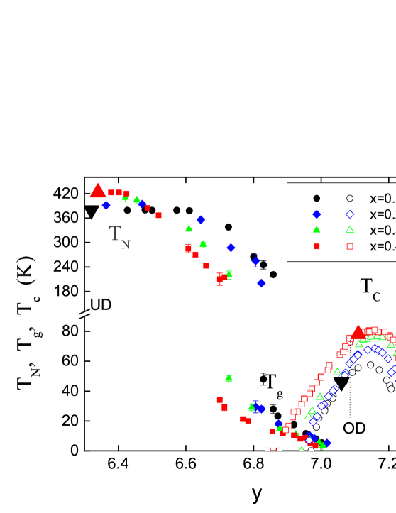
The multitude of different control parameters for emphasizes the importance of measuring their effects in isolation. Here we measure both and orbital splitting in (CLBLCO), using resonant inelastic x-ray scattering (RIXS). CLBLCO, whose phase diagram is shown in Fig. 1, is a compound which allows the tuning of structural parameters independently of the hole doping. Its structure is almost identical to YBCOGoldschmidt93 , but it is tetragonal and its chain layers are not ordered. The oxygen content controls the number of doped holes, only slightly affecting the lattice parameter. In complimentary fashion, Ca/Ba content changes only structural parameters such as bond length , buckling angles , and apical distance , while keeping the net valence fixed Sanna09 . Additionally, the entire doping range can be spanned from undoped to overdoped for all values of . Therefore, tunes both (through and ) and orbital splitting (through ) over the whole phase diagram. Moreover, disorder in CLBLCO was found to be -independent based on the line-widths measured by techniques ranging from high resolution powder x-ray diffraction Agrestini14 , Cu, Ca, and O nuclear magnetic resonance Marchand05 ; Keren09 ; Amit10 ; Cvitanic14 , phonon Wulferding14 , and ARPES Drachuck14 .
Intriguingly, both , as measured in undoped CLBLCO samples, and , were found to increase with by as much as 40%. In fact, the energy scale of the entire phase diagrams, including the magnetic, spin glass, and superconducting parts, scale with Ofer06 ; Ofer08 . Such scaling was attributed to a superconductivity governed by Ofer06 ; Ofer08 ; Drachuck14 ; Wulferding14 . However, in the optimally doped samples, and the possible effects of the apical oxygen distance, are not known. Measuring those are the main objective of this work.
Recent milestones in the technique of resonant inelastic (soft) x-ray scattering (RIXS) have been the measurement of dispersive magnetic excitations in superconducting cuprates and iron pnictidesBraicovich09 ; Braicovich10 ; LeTacon11 ; Zhou13 ; Dean13 . This, together with single-crystal CLBLCO growths Drachuck12 , have allowed us to measure how varies with in both underdoped and optimally doped CLBLCO samples. The momentum dependence provided by RIXS enables the precise determination of based on the spin-wave dispersion. Fortuitously, the same probe is also sensitive to the orbital excitations Ghiringhelli04 . Here we measure of both effects simultaneously on CLBLCO single crystals. We also use x-ray absorption spectroscopy (XAS) to verify that the effective hole dopings are indeed the same when we compare families with different .
We find that has a positive, but not proportional, correlation with . The and splittings also increase with , but we could not precisely isolate the excitation. We nevertheless determine that in this system has a greater contribution (treating it as the independent variable) to the change in , compared to the out-of-plane orbital effectOhta91 ; Pavarini01 ; Sakakibara10 ; Kuroki11 ; Sakakibara12 ; Yoshizaki12 . We also observed that the change in is very similar in the undoped and doped samples, and the slope of the - relation is identical to that of YBCO under pressure. The RIXS spectra also revealed unexpected features, including a peak at 0.8 eV, and energy dispersive excitations.
The paper is organized as follows. Section II describes the experimental details. Presentation and analysis of the RIXS data are divided into the sections: (III) RIXS of underdoped samples, with focus on the spin excitations; (IV) RIXS of doped samples; and (V) , or “crystal field” orbital excitations. Section VI is a discussion of the context of these results, and Section VII is the conclusion. Analysis of the doping from the O -edge and Cu -edge x-ray absorption spectra is provided in the Appendix.
II Experimental Details
( single crystals were grown using the traveling float-zone method Drachuck12 . For each of =0.1 and =0.4, the under-doped (UD) samples (in y) were prepared by annealing in argon. The near-optimally doped (OD) samples were first annealed in flowing oxygen, followed by 100 Atm oxygen pressure for a period of two weeks. The oxygen content for the OD samples was confirmed by iodometric titration. The oxygen content for UD sample was set based on the procedures used for powders so as to be in the antiferromagnetically long-range ordered phaseOfer06 . The ’s of the and OD samples were measured by magnetic susceptibility using a SQUID magnometer. They were K, and K respectively, indicating a close to optimal doping condition. The place of the samples in the phase diagram is shown in Fig. 1.
Soft x-ray absorption spectroscopy (XAS) and RIXS measurements were conducted at the ADRESS beamline Strocov09 at the Swiss Light Source of the Paul Scherrer Institut. The sample environment was 10 K in vacuum. The sample surfaces were cleaved -axis faces, mounted such that the - (or equivalent -) axis was in the horizontal scattering plane. For XAS, to obtain incident polarization approximately parallel to the -axis, the sample was rotated to 10∘ from the grazing incidence condition. Refer to the Appendix for the detailed XAS results.
RIXS spectra were measured in the horizontal scattering plane. Measurements were done for both horizontally and vertically polarized incident beams, corresponding to and polarizations respectively. The incident energy was set to the first main peak in the Cu XAS at 932 eV. The detector was fixed such that the two-theta scattering angle with respect to the incident beam was 130∘. Throughout this article, we refer to the in-plane momentum transfer in reciprocal lattice units of 2/, where is the lattice constant of the crystal. We define as the component of the total momentum change of the photon which is parallel to the sample plane Braicovich09 . Our sign convention is grazing incidence corresponding to negative . The variation of with each Ofer08 is accounted for in calculating , but is not significant on the -scale. In our scattering configuration is always along the (1 0 0) direction, and its magnitude is changed by rotating the sample away from specular reflection. Therefore the total momentum transfer is Q=(, 0, ) in tetragonal notation. The grazing incidence condition was used to calibrate the position. This calibration was found to be valid by measuring vs. dispersion for both positive and negative (see Section III).
III Magnons in Underdoped Samples
Typical RIXS spectra for the UD samples are compared in Fig. 2 for and . The various panels of Fig. 2 zoom in on different energy scales. The intensities are normalized to match at the strong peak in Fig. 2(b), and the energies are shifted so that the quasielastic peaks in Fig. 2(c) are centered at zero. Fig. 2(a) shows the relatively high-energy part of the spectra. First, we note that the and tails going down from 5 eV overlap closely. Secondly, there is a peak at around 4.5 eV which is in the energy range of charge transfer excitations across the Hubbard gap. The feature is shifted to higher energy for , and is also present in the doped samples. A doping-independent feature at similar energy was studied in LSCO with Cu -edge RIXS Ellis11 . Fig. 2(b) is an overall view of the spectra including both the intense peak encompassing the excitations between and eV, and the lower energy peaks, which are much lower intensity, but still visible on this scale. Comparison of the and spectra over a broad range reveals that generally, most of the excitations are at slightly higher energy for . This increased energy is ubiquitous both for the magnon excitations covered in this and the following section, and for the excitations in Section V. We note that both the high energy tails in Fig. 2(a), and the quasielastic peaks in Fig. 2(c), are aligned in energy for the two samples. We will later show that the magnon and excitation energy increases can be directly attributed to the change in lattice parameters.
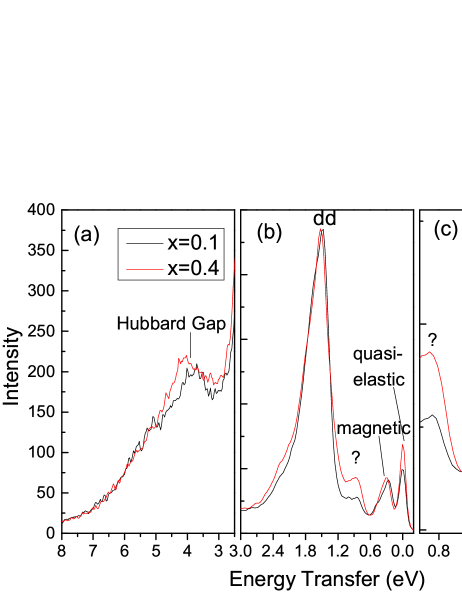
Fig. 2(c) zooms in on the low energy range. At zero energy is a quasielastic peak, which depends on a combination of finite -resolution of the instrument and the crystal mosaic of the sample. In our analysis, the energy scale of each spectra is shifted according to the center energy of the quasielastic peaks. In similar measurements done by Braicovich et al. Braicovich10 for , in which the quasielastic peak was much lower than it is here, a feature at around 80-90 meV was observed, with about a fifth of the magnon intensity. This was attributed to a resonantly enhanced optical phonon. We did not detect such a phonon and it is not included it in our analysis.
The peak associated with magnons is found in the 0.2-0.4 eV range of Fig. 2(c). Comparison of the data for (red) and (black) clearly shows that the peak is shifted to higher energy. Thus the main result that is higher in the sample than in the samples is clearly evident already in the raw data.
There is also a peak at eV. Its intensity is highest (comparable to the magnetic peak) at negative for polarized scattering, but can be seen elsewhere (see Fig. 3) and is always stronger for the sample. Where it is large, it was incorporated into our fitting for the magnons, described below. It has only slight dispersion of eV, unlike the new mode recently observed by Lee et al.Lee14 . It would be surprising if the eV peaks were one of the three excitations, which are expected to be above 1.5 eVSala11 . On the other hand, a excitation in the chain layer would be more plausible. Since half of the non-apical oxygen ligands around each Cu atom are missing in the chain, the Coulomb energy cost for a chain excitation should also be about half of a plane excitation, which corresponds to this eV.
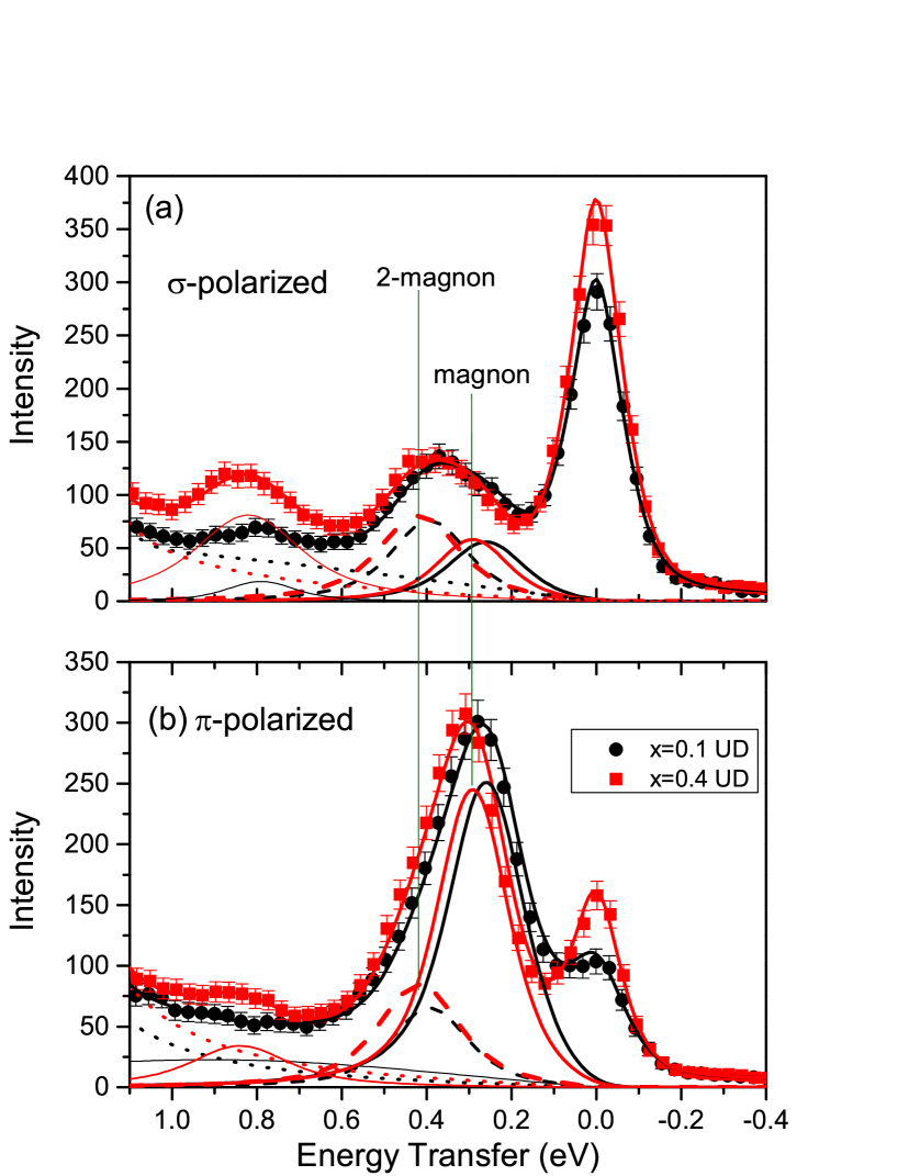
A sample pair of spectra corresponding to the and polarizations at the same are shown in Fig. 3(a) and (b). To extract the magnon energies, fitting was done over the range shown in Fig. 3. Each spectrum was modeled as a sum of quasielastic peak, magnon, 2-magnon, with (when visible) an additional peak at 0.8 eV, and a tail from the excitations. The spectral weight of the 2-magnon relative to the magnon is generally different for the and polarizations, resulting in a shift in the peak energy for the different polarizations. As in Ref. 33, the fitting is done for both polarizations simultaneously. The energies and widths of the magnon and 2-magnon peaks were constrained to be the same for both polarizations, as indicated by the vertical lines in Fig. 3. The lineshapes as a function of energy used for all of the excitations was a damped harmonic oscillator response in the form of a Lorentzian, weighted according to “detailed balance” :
| (1) | ||||
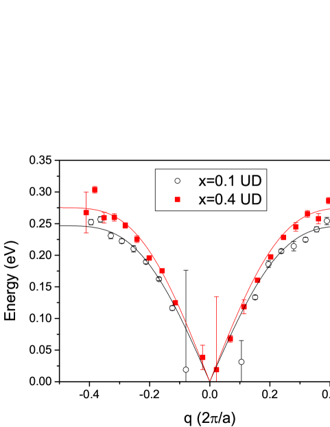
where is the sample temperature, is Boltzmann’s constant and fit parameters and are the energy and intrinsic width respectively. Each was then convolved with a Gaussian representing the resolution function of the spectrometer, to produce the components shown in Fig. 3. The fits for all spectra (more than 80) were excellent and are shown in the Supplementary materials SupMat . The dispersion of for the magnon components is plotted in Fig 4. The horizontal -axis for each sample was corrected by a slight shift (0.013 for =0.1 and 0.022 for =0.4) to make each dispersion symmetrical about the origin.
The dispersions are fit to a theoretical expression for acoustic-mode dispersion in the double layer cuprate YBCO Hayden96 :
| (2) |
for in-plane magnetic exchange , with interplane coupling set to 15 meV, and . There is also in principle an optical modeHayden96 , but it resides quite close to the acoustic mode, except at low , where the errorbars are high. In our fitting, was fixed at 15 meV (which is similar to YBCO Hayden96 ), so the only free parameter was . The fits are shown as the lines in Fig. 4. Eq. 2 captures the non-linearity of the data, particularly well on the negative side. The resultant values were meV for and for .
These values should be compared with detailed calculations done by Petit and Lepetit for optimally doped CLBCOPetit09 . Those yielded mean values of meV for and meV for . The results are in excellent agreement between theory and experiment, while there is a meV difference for . We show in the next section that the dispersion of the UD and OD samples are similar.
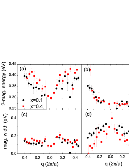
The other fit parameters are plotted in Fig. 5(a)-(d). In Fig. 5(a), the 2-magnon energies at low are close to eV. This magnitude is within the range of the recent 2-magnon Raman study in this material by Wulferding et al. Wulferding14 , who measured energies of eV in various samples. In addition, the sign and magnitude of dispersion of the 2-magnon of about eV in Fig. 5(a) is reasonably consistent with the 80 meV measured with O -edge RIXS by Bisogni et al.Bisogni12 in (see Figure 6 of Ref. 44). Fig. 5(b) plots the ratio of the intensities of the 2-magnon to the 1-magnon components. They fall on the same curve for and , which is expected since the excitations in both should have the same symmetries.
Fig. 5(c) and (d) show the intrinsic widths for the magnon and 2-magnon, which are 100-150 meV and meV respectively. These are wider than expected. The 2-magnon widths observed in the Raman study Wulferding14 were only 100 meV, while the magnon width is expected to be resolution limited on this scale. It is not clear if the large width originates in the fitting or sample. There is some intrinsic disorder in the site occupation between Ca, Ba, and La atoms, which could be a potential cause of an intrinsic magnon width. But if so, we note that the widths of =0.1 and =0.4 are about the same, indicating that does not affect disorder. Nevertheless, our analysis: (1) fit all of the data excellently with minimal number of parameters, (2) resulted in a realistic dispersion curve with values which are in good agreement with Ref. 45, and (3) 2-magnon energies at low are consistent with the 2-magnon energies measured with Raman scattering Wulferding14 , and (4) 2-magnon dispersion is consistent with O -edge value for from Ref. 44.
IV Paramagnons of Optimally Doped Samples
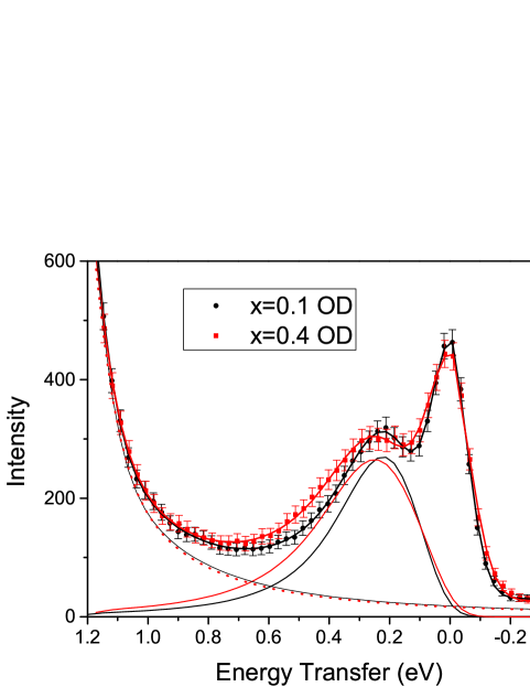
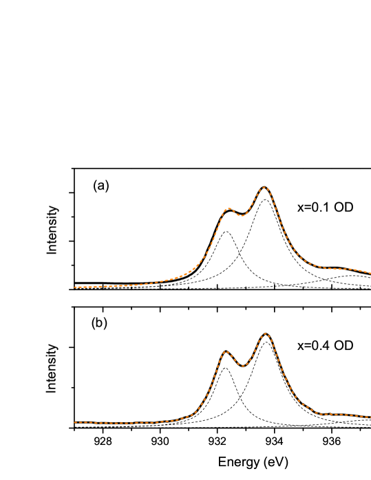
Here we estimate the change in in the superconducting samples. For doped cuprates, Le Tacon et al. found that the lifetime broadening of the spin excitations make the widths too broad to distinguish between magnon and 2-magnon, and instead they are replaced by a single “paramagnon” peak LeTacon11 . A typical spectrum for the OD CLBLCO samples is shown in Fig. 6. As in Ref. 33 we replaced the magnon and 2-magnon with a single magnetic component, retaining the lineshape of Eq. 1. Only the elastic intensity, “paramagnon” peak, and tail from the were included in the fits. Most of the ’s measured were positive, and there were no strong 0.8 eV peaks. Since the peak position is generally different for and polarizations, due to different weights of the 2-magnon and magnon contributions (as seen in Fig. 3), both could not be fit simultaneously with one peak. We therefore chose to use only the polarization. The single peak of Eq. 1 plus background fit quite well to the data; fits to all of the spectra are shown in the Supplementary materials SupMat . As seen in both the fits and raw data of Fig. 6, the paramagnon for is shifted with respect to and extends to higher energy, which was also typical for the other ’s. We note that in Fig. 6 the tails from high energy are the same for and .
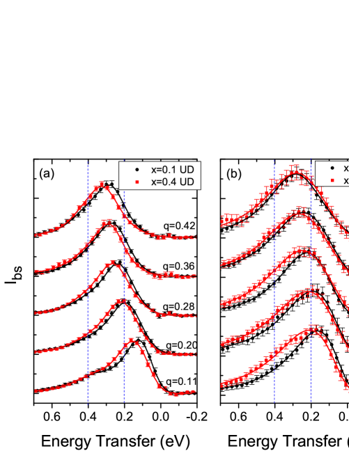
A series of spectra for progressively higher are plotted in Fig. 7, for (a) the UD samples and (b) the OD samples. The spectra in Fig. 7(a) for the UD samples were obtained by subtracting all of the fitted components (see Section III) from the raw data, save for the magnon and 2-magnon contributions. The same procedure is applied to the OD samples in Fig. 7(b), by subtracting the non-magnetic contribution. The positions are similar for Fig. 7(a) and Fig. 7(b). Both pairs of spectra in Fig. 7(a) and (b) are centered below 0.2 eV at low (bottom spectra), and by =0.4 (top spectra) they dispersed to 0.3 eV. This similarity suggests that the comparison for the UD spectra, which is generally easier to precisely determine, is also valid for the superconducting case. It also would seem to argue against the scenario of intraband excitations (as opposed to paramagnons) which was recently proposed by Benjamin et al.Benjamin14 , since the OD and UD spectra have the same energies.
The value of cannot directly be determined from the “paramagnon” spectra. The fitted energy parameter of the asymmetric lineshape in Eq. 1 does not have the same well-defined meaning as in the two-peak, two-polarization fits used in section III. This is because the peak fitted-for here encompasses both magnon and 2-magnon components, weighted by some unknown amount depending on scattering cross-section for each (one can refer to Fig. 5(b) for the UD case). Instead, for comparison purposes we use the center-of-mass, namely, the statistical mean energy = of the background-subtracted magnetic spectra of Fig. 7(b). While this definition is arbitrary, for a given , it should be roughly proportional to for any two samples, since both magnon and 2-magnon energies are proportional to .
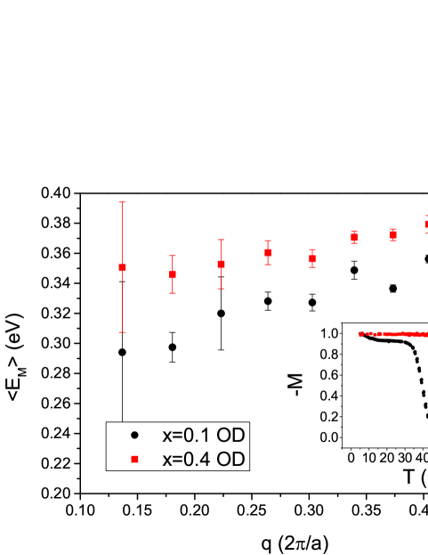
is plotted as a function of in Fig. 8 for (black circles) and (red squares). For all but the last, it is higher for . The average over these points, , is eV for and eV for . Assuming proportionality, we interpret this as a 9% increase in from to . By comparison, the percentage increase for the (more precisely determined) ’s of the UD samples in Section III is 11.7%. Considering the broad widths of the OD spectra and the somewhat cruder method of estimating their , this estimated increase is quite close to the UD case.
In the inset of Fig. 8 we present the negative magnetization measurements of the two superconducting samples used for RIXS. There is a clear difference in their . The main observation of this work is that the sample with higher also has higher . It was also demonstrated here that RIXS can distinguish samples with small differences in even in the optimally doped case.
V Crystal Field () Excitations
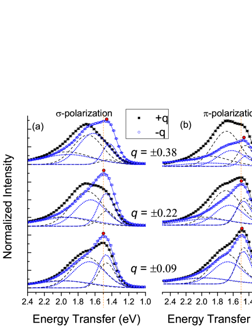
The spectra of our UD samples were generally sharper than for our OD samples, so we focus on the former. The excitation spectra of the UD samples are plotted in Fig. 9 for selected ’s for the =0.1 sample. The spectra of the =0.4 sample was qualitatively similar in the main features, but with slightly higher energies (see Fig. 2(b)). All of the spectra and fittings for the full range of ’s are presented in the Supplementary materialsSupMat . The centering of the quasi-elastic peaks of all of the spectra are also shown in the Supplementary materials to be accurate within 10 meV. At least two peaks are clearly resolved, at 1.5 eV and 1.7 eV, with the intensity of the 1.7 eV peak becoming relatively stronger with increased . We fit the and polarized spectra simultaneously to a sum of Gaussians, constraining the parameters of widths and energies to be the same for both polarizations. Three Gaussians worked best. They are shown in Fig. 9. The zero energies are defined by the elastic peaks (see Section III). As can be seen in Fig. 9 the widths successively increased from the low to high energy peaks.
To assign the peaks, we refer to the work of Sala et al.Sala11 , who studied excitations with Cu -edge RIXS in a variety of cuprates. They found excellent agreement between the observed polarization and dependence, and their cross-section calculations. The compound studied in that work which is structurally similar to CLBLCO is the double-layer 123-cuprate (NBCO). In what follows, , , and refer to the energies of the orbital transitions , , and respectively. The NBCO spectra had two prominent peaks at 1.52 eV and 1.75 eV, which the authors of Ref. 42 assigned to and . was calculated to be 1.97 eV, but it was not visible in their spectra. As increased, the cross-section of the 1.75 eV peak increased relative to the 1.5 eV peak. These results, both the energies and cross-section -dependence are very close to what we observe for CLBLCO in Fig. 9. We therefore likewise assign the 1.5 eV peak to and the 1.7 eV peak to . Furthermore, the energy of the broad third Gaussian component in Fig. 9 happened to lie very close to 2 eV, with zone-averages (standard deviations) of 1.97(0.03) eV, and 2.00(0.1) eV, for =0.1 and =0.4 respectively. While this energy is in excellent agreement with calculations for in NBCOSala11 , and for YBCOMagnuson14 the broadness makes it difficult to identify with certainty.
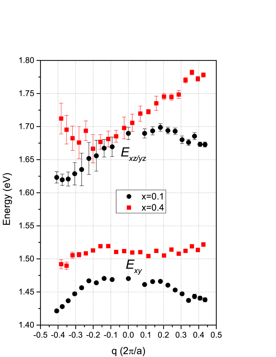
The -dependence of and are plotted in Fig. 10 for =0.1 and =0.4. Surprisingly, there appears to be some dispersion in the energies. The excitation for =0.1 shows flat dispersion near the zone center, up to around =0.2, but beyond this it exhibits negative dispersion of the order of 0.05 eV towards the zone boundary. This dispersion is quite symmetrical about =0, up to =0.35. The dispersion could also be seen from the raw data. In Fig. 9, the red circles mark the low-energy peaks of the negative branch. They also mark the positive branch, but it is harder to see for high , especially for -polarization. For the bottom two spectra, corresponding to =0.09 and =0.22, the peaks are aligned with the vertical dashed line, but by =0.38, the peak of the raw data is visibly shifted to the right of the line by about 50 meV. A non-zero dispersion suggests propagation of the orbital excitation. For , the excitation shows similar dispersion on the negative branch, but its magnitude is roughly halved. also shows dispersion, but is not symmetrical about =0. The fitted energies for =0.4 especially show a linear trend with a dispersion of almost 0.1 eV between . Unlike the dispersion, the dispersion is not obvious from the raw data itself due to the wider peaks, and only becomes apparent after the fittings. Although it seems counter-intuitive, asymmetric dispersion may happen in the presence of spin-orbit interaction. It has already been observed in the spin-wave of Fe ultrathin filmsZakeri10 , for example. But, as far as we know this would be the first observation of asymmetry in the dispersion of a excitation.
We can check whether scales properly with the lattice parameter. As pointed out by Sala et al.Sala11 . Averaging the energies of Fig. 10 over the zone yields, for (), 1.46 (1.52) eV and 1.69 (1.75) eV. The corresponding values for is =3.91 Å and for is =3.88 Å. This yields =5.1 remarkably close to the theoretical single-ion crystal field model’s value of =5.
VI Discussion
Analysis of the UD spectra in Section III provided explicit values of 120 meV (=0.1) and 134 meV (=0.4). The corresponding for these values are 57 K and 80 K respectively Ofer06 . In section IV, we found that the change in for doped samples is comparable to the undoped case, and the two dopings furthermore exhibit very similar dispersions of the spin-excitation spectra (refer to Fig. 7). It is therefore justified to apply the UD values of to the superconducting case, as has been assumed to be valid in other worksMallet13 ; Wulferding14 . With as an implicit parameter we find that =1.64 K/meV. This is the same order of magnitude of the average slope obtained from the study of Munoz et al.Munoz00 of several cuprates having different numbers of layers ( K/meV) . It is even more closely aligned with the initial slope for YBCO under hydrostatic pressure ( K/meV) Mallet13 . Moreover, the increase of of 11.7% from =0.1 to =0.4 determined for the UD samples in Section III is in close agreement with the estimation of 11.9% we obtain by using a simple ruleOfer08 . In addition, scales as expected with distances. These results indicate that the in-plane energies and depend purely on in-plane parameters, without secondary effects arising from different Ca/Ba ratios. We speculate that the peak, which we could not properly resolve, behaves as expected from the lattice parameters variations between different CLBLCO families.
Whether likewise depends only on the in-plane parameters is not a priori clear, since the out-of-plane lattice parameter , and apical oxygen distance are also functions of . In fact, a number of studiesOhta91 ; Pavarini01 ; Sakakibara10 ; Kuroki11 ; Sakakibara12 ; Yoshizaki12 ; Johnston10 focused on the effect of and on in various cuprate systems. We now assess the relative importance that these have for .
Since YBCO and CLBCO share very similar structure and lattice parameters, it is relevant to compare the two. The values of observed in the pressure-dependence of YBCO on one hand, and in the -dependence of CLBLCO observed here on the other, are very similar. Hydrostatic pressure compresses the -axis, decreasing the apical oxygen distance and increasing . In contrast, when increasing (and ) in CLBLCO, increases Ofer08 . That is the same for YBCO and CLBLCO, in spite of changing in the opposite sense, leads us to conclude that variations do not play a major role here in determining .
Another way to reach this conclusion for CLBLCO is to estimate the effect of the change in on by comparing with other studies. A sensitivity of roughly 30 K/, was shown across various cuprates by Johnston et al.Johnston10 (see Figure 1 of Ref. 49). In CLBLCO powder, as increases from 0.1 to 0.4, increases by 0.05 Ofer08 . On that basis, the effect of on in CLBLCO would be less than K.
A similar effect of on results from the theoretical calculations of () by Sakakibara et al.Sakakibara10 . They calculated the Eliashberg eigenvalue which sets a limit on . From their calculations, an upper limit of 125 K/ can be set, which is still too small to account for the variations in CLBLCO.
Taken together, the above comparisons suggest that in CLBLCO has very little impact on . By eliminating this out-of-plane influence, it becomes more likely that the change in observed between different families of CLBLCO is due to variations in . While increases by 40% (Fig. 1) from =0.1 to =0.4, as measured by RIXS only increases by %. From other methods, the corresponding increase in for samples with the same in-plane hole underdoping was determined to be: from the 2-magnon Raman peaks Wulferding14 , from angle resolved photoemission spectroscopyDrachuck14b , in ab initio calculations Petit09 , and 40% by SR with extraction of from Ofer06 . With the exception of the latter, these estimates were all considerably less than the increase in . This suggests that the dependence of is not proportional, as predicted by some exchange-driven theoriesScalapino98 ; Sushkov04 . If a linear relationship extends down to =0, it would imply a threshold for superconductivity.
VII Conclusion
To review, we measured the O -edge and Cu -edge XAS, and RIXS spectra at the Cu -edge, in both underdoped and optimally doped CLBLCO single crystals of and families which have different .
From the electronic structure of the XAS spectra, similar hole dopings in the superconducting samples of the different families were confirmed. As it turns out, doping does not have a critical effect on the magnon dispersion, besides a broadening of the peaks. The relative change in magnetic energies between =0.1 and =0.4 are furthermore similar for the doped and undoped cases. This demonstrates that RIXS can distinguish between samples of slightly different even in the doped case.
The main excitations were also examined and unexpectedly dispersion of up to 0.05 eV was observed, raising the possibility that these orbital excitations can propagate. More intriguingly, the dispersion of the excitation from the orbit appeared to be asymmetric about =0. Higher resolution studies would be needed to clarify this dispersion. In the UD samples, an additional 0.8 eV peak was observed, and attributed to a excitation in the chain layer.
Finally, there is a positive correlation between and with a slope consistent with the pressure dependence of both parameters in YBCO. The measured spin-wave energies change with by an amount that would be expected from purely in-plane lattice constants change. Furthermore, it is concluded that the apical oxygen distance does not change enough with to have a significant effect on . These points suggest that the variation with in CLBLCO is purely an in-plane effect driven by orbital overlaps.
Acknowledgements
The RIXS and XAS measurements were performed on the ADRESS beamline at the Swiss Light Source, Paul Scherrer Institut, Villigen, Switzerland. Part of this work has been funded by the Swiss Nationional Science Foundation and its Sinergia network Mott Physics Beyond the Heisenberg (MPBH) model. J.P. and T.S. acknowledge financial support through the Dysenos AG by Kabelwerke Brugg AG Holding, Fachhochschule Nordwestschweiz, and the Paul Scherrer Institut. We acknowledge financial support from the Israeli Science Foundation grant 249/10 for JB and DE, and grant 666/13 for GD, RO, GB, and AK. The research leading to these results has received funding from the European Community’s Seventh Framework Programme (FP7/2007-2013) CALIPSO under grant agreement no. 312284. We also thank Daniel Podolsky for helpful discussions.
Appendix: XAS analysis
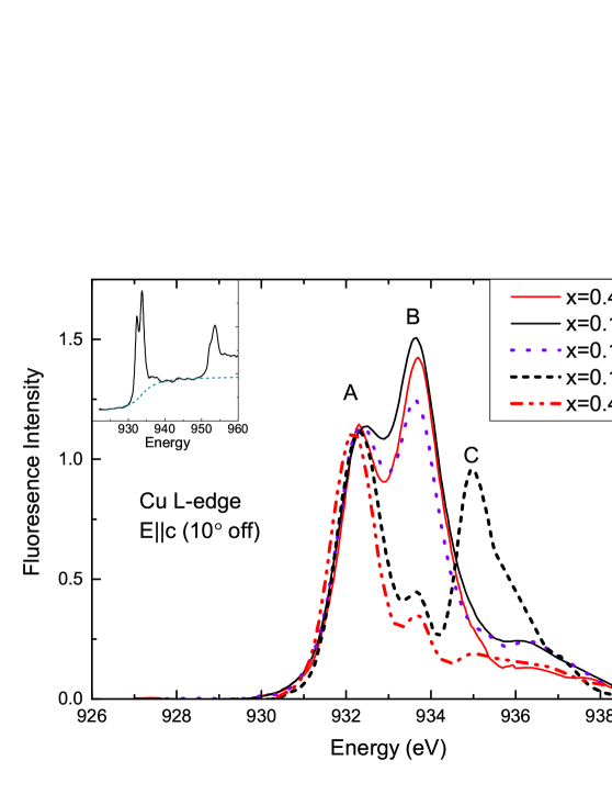
In addition to determining the resonance energy needed for RIXS, XAS also provides valuable information about the number of holes present in our samples. We measured the XAS of the single crystal =0.4 OD and UD, and =0.1 OD, and UD samples. In addition, an =0.1 sample of intermediate doping (MD), estimated to be just before the onset of superconductivity, was measured. We used much of the same approach for analysis as was used by Agrestini et al.Agrestini14 for treatment of CLBLCO powder. The clearest and most systematic spectra were at the Cu -edge when the electric field is polarized along the -axis (with a 10∘ misalignment from axis), and at the O -edge absorption when the electric field is polarized parallel to the -plane. These are shown in Fig. 11 and Fig. 12 respectively, after subtracting a background in the form of an inverse tangent function as shown in the insets. Referring to Fig. 11, the data were normalized so as to have the same maxima of peak for all samples, which comes from the Cu Cu transition Nucker95 ; Agrestini14 .
The low energy edges of the peaks of all samples match perfectly, with the exception of =0.4 UD whose peak is shifted to slightly lower energy. The second peak is at the same energy for all samples. It corresponds to the same absorption process as , but in the presence of a ligand hole, namely Cu Cu Nucker95 ; Agrestini14 . It is clear that peak becomes less and less intense as the doping decreases, but is roughly the same between =0.1 and =0.4 for identical nominal dopings. A third peak appears for the UD samples 3 eV from peak . It is quite strong for =0.l but is only a small bump for =0.4. Such a peak is associated with charge transfer excitations to the upper Hubbard bandFink94 ; Merz98 . A satellite peak around that energy has been related to the chain layer in the 123-compoundsSalluzzo08 .
The number of holes can be determined from the relative peak intensity Agrestini14 ; Kuiper88 . The spectra were fitted to three Lorentzians, as shown in Fig. 13 for the OD samples. The ratio of the areas of the components, , for OD and samples were and respectively, indicating identical hole doping for both samples. Additionally, we can estimate and the total number of holes in a unit cell including chains and planes, . Roughly 20% of is expected to be in each plane Nucker95 . From the measured of the OD samples, combined with the phase diagram for powders (see Fig. 1) Ofer08 , we obtain =7.06 and 7.11 for the =0.4 and =0.1 samples respectively. This is near the top, but slightly to the left of the peak of the superconducting domes. We then estimate the amount of holes using the relation Agrestini14 . Using that as a reference, and assuming the area ratios are proportional to , we can estimate and of the UD and MD samples. A summary of the intensity ratios, estimated , and estimated for the various samples is tabulated in table 1. We note that 6.32-6.34, placing it well into the antiferromagnetic long-range ordered phase (Fig. 1). Likewise, , which is consistent with the iodometric titration result of 6.92 for this sample.
| Sample | |||
|---|---|---|---|
| =0.4 OD | 0.86 | 7.11 | |
| =0.1 OD | 0.81 | 7.06 | |
| =0.1 MD | 0.69 | 6.94 | |
| =0.1 UD | 0.07 | 6.32 | |
| =0.4 UD | 0.09 | 6.34 |
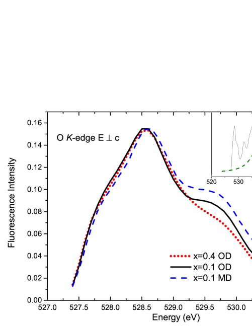
To further compare the relative hole densities, the normalized oxygen -edge spectra is plotted in Fig. 12. It was measured for the =0.1 OD, =0.4 OD, and =0.1 MD samples. The effect of the holes may be seen by inspection of the positions of the low-energy peak of the O -edge spectra. Shifts in this oxygen “pre-edge” energy track the shift in Fermi level with hole doping Kuiper88 ; Nucker95 . This shift is a direct consequence of the filling (or emptying) of the bands. From Fig. 12, the low-energy oxygen -edges overlap almost exactly for the and OD samples. In contrast, the edge of the MD spectrum shifts by about 0.07 eV. Based on the result shown for YBCO in Ref. 52, the shift would correspond to a change in doping of . This is of the same order of magnitude as between the OD and MD samples in table 1. The almost overlapping edges for the =0.1 and =0.4 OD samples is therefore a second confirmation of identical number of holes, and furthermore indicates that the amount holes in the plane layer are the same.
References
- (1)
- (2) D. J. Scalapino, Rev. Mod. Phys. 84, 1383 (2012).
- (3) P. W. Anderson, Science 235, 1196 (1987).
- (4) D. J. Scalapino and S. R. White, Phys. Rev. B 58, 8222 (1998).
- (5) O. P. Sushkov and V. N. Kotov, Phys. Rev. B 70, 024503 (2004).
- (6) D. Muñoz, F. Illas and I. de P. R. Moreira, Phys. Rev. Lett. 84, 1579 (2000).
- (7) D. Muñoz, I. de P. R. Moreira and F. Illas, Phys. Rev. B 65, 224521 (2002).
- (8) B. P. P. Mallett, T. Wolf, E. Gilioli, F. Licci, G. V. M. Williams, A. B. Kaiser, N. W. Ashcroft, N. Suresh and J. L. Tallon, Phys. Rev. Lett. 111, 237001 (2013).
- (9) M. P. M. Dean, A. J. A. James, A. C. Walters, V. Bisogni, I. Jarrige, M. Hücker, E. Giannini, M. Fujita, J. Pelliciari, Y. B. Huang, R. M. Konik, T. Schmitt and J. P. Hill, Phys. Rev. B 90, 220506(R) (2014).
- (10) M. W. McElfresh, M. B. Maple and K. N. Yang, Appl. Phys. A 45, 365 (1988).
- (11) N. Mori, C. Murayama, H. Takahashi, H. Kaneko, K. Kawabata, Y. Iye, S. Uchida, H. Takagi, Y. Tokura, Y. Kubo, H. Sasakura and K. Yamaya, Physica C 185-189, 40 (1991).
- (12) S. Koltz, W. Reith and J. S. Schilling, Physica C 172, 423 (1991).
- (13) S. Sadewasser, J. S. Schilling, A. P. Paulikas and B. W. Veal, Phys. Rev. B 61, 741 (2000).
- (14) Y. Ohta, T. Tohyama and S. Maekawa, Phys. Rev. B 43, 2968 (1991).
- (15) E. Pavarini, I. Dasgupta, T. Saha-Dasgupta, O. Jepsen and O. K. Andersen, Phys. Rev. Lett. 87, 047003 (2001).
- (16) H. Sakakibara, H. Usui, K. Kuroki, R. Arita and H. Aoki, Phys. Rev. Lett. 105, 057003 (2010).
- (17) K. Kuroki, Journal of Physics and Chemistry of Solids 72, 307 (2011).
- (18) H. Sakakibara, H. Usui, K. Kuroki, R. Arita and H. Aoki, Phys. Rev. B 85, 064501 (2012).
- (19) R. Yoshizaki, T. Yamamoto, H. Ikeda and K. Kadowaki, Journal of Physics: Conference Series 400, 022142 (2012).
- (20) S. Raghu, R. Thomale and T. H. Geballe, Phys. Rev. B 86, 094506 (2012).
- (21) D. Goldschmidt, G. M. Reisner, Y. Direktovitch, A. Knizhnik, E. Gartstein, G. Kimmel and Y. Eckstein, Phys. Rev. B 48, 532 (1993).
- (22) S. Sanna, S. Agrestini, K. Zheng, R. de Rezni and N. L. Saini, European Physics Letters 86, 67007 (2009).
- (23) S. Agrestini, S. Sanna, K. Zheng, R. de Renzi, E. Psuceddu, G. Concas, N. L. Saini and A. Bianconi, Journal of Physics and Chemistry of Solids 75, 259 (2014).
- (24) S. Marchand, Ph. D. thesis, Université Paris, Paris (2005).
- (25) A. Keren, New Journal of Physics 11, 065006 (2009).
- (26) E. Amit and A. Keren, Phys. Rev. B 82, 172509 (2010).
- (27) T. Cvitanić, D. Pelc, M. Požek, E. Amit and A. Keren, Phys. Rev. B 90, 054508 (2014).
- (28) Dirk Wulferding, Meni Shay, Gil Drachuck, Rinat Ofer, Galina Bazalitsky, Zaher Salman, Peter Lemmens and Amit Keren, Phys. Rev. B 90, 104511 (2014).
- (29) G. Drachuck, E. Razzoli, R. Ofer, G. Bazalitsky, R. S. Dhaka, A. Kanigel, M. Shiand A. Keren, Phys. Rev. B 89, 121119(R) (2014).
- (30) R. Ofer, G. Bazalitsky, A. Kanigel, A. Keren, A. Auerbach, J. S. Lord and A. Amato, Phys. Rev. B 74, 220508(R) (2006).
- (31) R. Ofer, A. Keren, O. Chmaissem, A. Amato, Phys. Rev. B 78, 140508 (2008).
- (32) L. Braicovich, L. J. P. Ament, V. Bisogni, F. Forte, C. Aruta, G. Balestrino, N. B. Brookes, G. M. D. Luca, P. G. Medaglia, F. M. Granozio, M. Radovic, M. Salluzzo, J. van den Brink, and G. Ghiringhelli, Phys. Rev. Lett. 102, 167401 (2009).
- (33) L. Braicovich, J. van den Brink, V. Bisogni, M. M. Sala, L. J. P. Ament, N. B. Brookes, G. M. De Luca, M. Salluzzo, T. Schmitt, V. N. Strocov and G. Ghiringhelli, Phys. Rev. Lett. 104, 077002 (2010).
- (34) M. Le Tacon, G. Ghiringhelli, J. Chaloupka, M. Moretti Sala, V. Hinkov, M. W. Haverkort, M. Minola, M. Bakr, K. J. Zhou, S. Blanco-Canosa, C. Y. T. Song, G. L. Sun, C. T. Lin, G. M. De Luca, M. Salluzzo, G. Khaliullin, T. Schmitt, L. Braicovich, B. Keimer, Nature Physics 7, 725 (2011).
- (35) K-J. Zhou, Y-B. Huang, C. Monney, X. Dai, V. N. Stocov, N-L. Wang, Z-G. Chen, C. Zhang, P. Dai, L. Patthey, J. van den Brink, H. Ding and Thorsten Schmitt, Nat. Comm. 4, 1470 (2013).
- (36) M. P. M. Dean, G. Dellea, R. S. Springell, F. Yakhou-Harris, K. Kummer, N. B. Brookes, X. Liu, Y-J. Sun, J. Strle, T. Schmitt, L. Braicovich, G. Ghiringhelli, I. Bozovic and J. P. Hill, Nat. Mat. 12, 1019 (2013).
- (37) G. Drachuck, M. Shay, G. Bazalitsky, R. Ofer, Z. Salman, A. Amato, C. Niedermayer, D. Wulferding, P. Lemmens and A. Keren, Journal of Superconductivity and Novel Magnetism doi 10. 1007/s10948-012-1669-z (2012).
- (38) G. Ghiringhelli, N. B. Brookes, E. Annese, H. Berger, C. Dallera, M. Grioni, L. Perfetti, A. Tagliaferri and L. Braicovich, Phys. Rev. Lett. 92, 117406 (2004).
- (39) V. N. Strocov, T. Schmitt, U. Flechsig, T. Schmidt, A. Imhof, Q. Chen, J. Raabe, R. Betemps, D. Zimoch, J. Krempasky, X. Wang, M. Grioni, A. Piazzalunga and L. Patthey, Journal of Synchrotron Radiation 17, 631 (2009).
- (40) D. S. Ellis, Jungho Kim, H. Zhang, J. P. Hill, G. Gu, S. Komiya, Y. Ando, D. Casa, T. Gog and Y. J. Kim, Phys. Rev. B 83, 075120 (2011).
- (41) See Supplement Material at [URL will be inserted by publisher].
- (42) W. S. Lee, J. J. Lee, E. A. Nowadnick, S. Gerber, W. Tabis, S. W. Huang, V. N. Strocov, E. M. Motoyama, G. Yu, B. Moritz, H. Y. Huang, R. P. Wang, Y. B. Huang, W. B. Wu, C. T. Chen, D. J. Huang, M. Greven, T. Schmitt, Z. X. Shen and T. P. Devereaux, Nature Physics 10, 883 (2014).
- (43) M. M. Sala, V. Bisogni, C. Aruta, G. Balestrino, H. Berger, N. B. Brookes, G. M. deLuca, D. Di Castro, M. Grioni, M. Guarise, P. G. Medaglia, F. M. Granozio, M. Minola, P. Perna, M. Radovic, M. Salluzzo, T. Schmitt, K. J. Zhou, L. Braicovich and G. Ghiringhelli, New Journal of Physics 13, 043026 (2011).
- (44) S. M. Hayden, G. Aeppli, T. G. Perring, H. A. Mook and F. Doğan, Phys. Rev. B 54, R6905 (1996).
- (45) V. Bisogni, L. Simonelli, L. J. P. Ament, F. Forte, M. Moretti Sala, M. Minola, S. Huotari, J. van den Brink, G. Ghiringhelli, N. B. Brookes and L. Braicovich, Phys. Rev. B 85, 214527 (2012).
- (46) S. Petit and M.-B. Lepetit, European Physics Letters 87, 67005 (2009).
- (47) D. Benjamin, I. Klich and E. Demler, Phys. Rev. Lett. 112, 247002 (2014).
- (48) M. Magnuson, T. Schmitt, V. N. Strocov, J. Schlappa, A. S. Kalabukhov and L.-C. Duda, Scientifc Reports 4, 7017 (2014).
- (49) Kh. Zakeri, Y. Zhang, J. Prokop, T. -H. Chuang, N. Sakr, W. X. Tang and J. Kirschner, Phys. Rev. Lett. 104, 137203 (2010).
- (50) S. Johnston, F. Vernay, B. Moritz, Z. -X. Shen, N. Nagaosa, J. Zaanen and T. P. Devereaux, Phys. Rev. B 82, 064513 (2010).
- (51) Gil Drachuck, Elia Razzoli, Rinat Ofer, Galina Bazalitsky, R. S. Dhaka, Amit Kanigel, Ming Shi and Amit Keren, Phys. Rev. B 89, 121119(R) (2014).
- (52) P. Kuiper, G. Kruizinga, J. Ghijsen, M. Grioni, P. J. W. Weijs, F. M. F. de Groot, G. A. Sawatzky, H. Verweij, L. F. Feiner and H. Petersen, Phys. Rev. B 38, 6483 (1988).
- (53) N. Nücker, E. Pellegrin, P. Schweiss, J. Fink, S. L. Molodtsov, C. T. Simmons, G. Kaindl, W. Frentrup, A. Erb and G. Müller-Vogt, Phys. Rev. B 51, 8529 (1995).
- (54) J. Fink, N. Nücker, E. Pellegrin, H. Romberg, M. Alexander and M. Knupfer, J. of Electron. Spec. and Related Phenom. 66, 395 (1994).
- (55) M. Merz, N. Nücker, P. Schweiss, S. Schuppler, C. T. Chen, V. Chakarian, J. Freeland, Y. U. Idzerda, M. Kläser, G. Müller-Vogt and Th. Wolf, Phys. Rev. Lett. 80, 5192 (1998).
- (56) M. Salluzzo, G. Ghiringhelli, J. C. Cezar, N. B. Brookes, G. M. De Luca, F. Fracassi and R. Vaglio, Phys. Rev. Lett. 100, 056810 (2008).