Coscattering in the Extended Singlet-Scalar Higgs Portal
Abstract
We study the coscattering mechanism in a simple Higgs portal which add two real singlet scalars to the Standard Model. In this scenario, the lighter scalar is stabilized by a single symmetry and acts as the dark matter relic, whose freeze-out is driven by conversion processes. The heavier scalar becomes an unstable state which participate actively in the coscattering. We find viable parameter regions fulfilling the measured relic abundance, while evading direct detection and big-bang nucleosynthesis bounds. In addition, we discuss collider prospects for the heavier scalar as a long-lived particle at present and future detectors.
1 Introduction
Coscattering DAgnolo:2017dbv or Conversion-driven freeze-out Garny:2017rxs is a thermal dark matter (DM) framework in which the dark matter relic abundance is determined by the freeze-out of inelastic conversions in the dark sector. In the typical coannihilation regime such processes are assumed to be rapid enough to keep the dark sector in chemical equilibrium (CE) even long after the freeze-out of the DM from the thermal plasma. In contrast, in the coscattering scenario the dark sector falls out of CE roughly once the conversion rates drop below the Hubble expansion rate. For previous studies of this mechanism in several different models see Refs. Cheng:2018vaj ; Garny:2018icg ; DAgnolo:2018wcn ; Brummer:2019inq ; Junius:2019dci ; DAgnolo:2019zkf ; Garny:2021qsr ; Herms:2021fql ; Heeck:2022rep ; Filimonova:2022pkj ; Heisig:2024xbh .
A typical feature of the coscattering regime is the presence of long-lived particles (LLP), because the small coupling strength between the relic and unstable dark partner required for a fast freeze-out of the conversions in turn implies a narrow decay with of the dark partner. Furthermore, the masses of the DM species must be highly degenerate, , as otherwise the Boltzmann suppression of the conversion rate leaves the coscattering mechanism inactive. Since the LLPs can couple much more strongly to the SM they are excellent candidates for direct detection of DM at present or future colliders Curtin:2018mvb ; Cottin:2024dlo ; Heisig:2024xbh .
In this paper, we study the coscattering mechanism in one of its perhaps simplest possible realizations,
a two real singlet-scalar model coupling to the SM through the Higgs portal Ghorbani:2014gka ; Casas:2017jjg . Here, the lighter scalar is stabilized by a discrete symmetry, while the second scalar
acts as the unstable dark partner. We find that the coscattering regime allows for DM masses at the
EW scale, while the dark partner constitutes a LLP with km.
The paper is structured in the following way. In Sec. 2 we present the model. In Sec. 3 we discuss the calculation of the relic abundance in its different regimes, paying special attention to the coscattering regime. In Sec. 4 we present the relevant experimental constraints and obtain results for the expected lifetimes of the LLP. Finally, we give some concluding remarks in Sec. 5.
2 Model
We consider the SM extended by two real singlet-scalars and . is taken to be the lighter scalar, which is stabilized by a symmetry under which , while the SM fields transform trivially Casas:2017jjg ; Ghorbani:2014gka . As a result, the scalars couple to the SM only via the Higgs field. The corresponding Lagrangian in the scalar mass basis (for more details see App. A) is given by
| (1) | ||||
where denotes the SM Higgs doublet and GeV the Higgs vacuum expectation value (vev). None of the new scalars acquire a vacuum expectation value.
In the following, we consider the set of independent model parameters and denote the mass difference between the scalars by . In the coscattering regime, the couplings and play a similar role to and are omitted for simplicity.
3 Coscattering or Conversion-driven freeze-out
In the coscattering regime we explicitly do not assume CE within the dark sector during the evolution of the DM number densities up to the point of freeze-out. As a result, the full coupled Boltzmann equations (cBE), assuming all possible interaction terms, have to be solved in order to obtain the correct DM relic abundance. In the following we introduce together with the typical definition of the DM yield , where denotes the entropy density.
3.1 Boltzmann equations
The cBE for and reads
| (2a) | ||||
| (2b) | ||||
where denotes the Hubble rate, stand for any SM particles, and for and respectively. The equilibrium yields are given by
| (3a) | ||||
| (3b) | ||||
where is the modified Bessel function of the second kind, the number of effective degrees of freedom associated to the entropy density . In contrast to the cBE for coannihilation, eqs. (2) explicitly contains the DM conversion rate
| (4) |
where and denote light SM states. The calculation of the relevant conversion cross sections together with their thermal average is presented in App. B. The second important conversion process is given by decays of the unstable partner with the thermally averaged decay rate Garny:2017rxs
| (5) |
We solve the above cBE using micrOMEGAs 5.3.41 Belanger:2001fz ; Alguero:2022inz , considering three separate sectors: i) the SM, ii) the DM candidate , and iii) a dark sector for . micrOMEGAs solves all the relevant average cross sections, including the two and three-body decay widths of considering Lorentz time effects. To quantify the impact of coscattering and compare the results obtained from the full cBE to the results assuming CE we use Alguero:2022inz
| (6) |
where (1 sector) is obtained using the darkOmega function of micrOMEGAs and (2 sectors) is obtained from darkOmegaN111In the present paper we did not make explicit use of the function defined in Alguero:2022inz , although part of the analysis in this section contemplates the information that could be obtained with that function.. The scaling of each process with the model parameters are listed in Table 1.
| Initial | Final | Scaling |
|---|---|---|
| 1 1 | 0 0 | |
| 2 2 | 0 0 | |
| 1 1 | 2 2 | |
| 1 2 | 0 0 | |
| 1 0 | 2 0 | |
| 2 | 1 0 |
3.2 Relic abundance
The basic characteristic of the conversion-driven freeze-out in the two scalar Higgs portal are:
-
1.
remains in CE with only through either (inverse) decays or coscattering processes .
-
2.
Annihilation processes involving can be neglected.
The first condition requires that is non-vanishing but small enough for the conversion processes not to surpass the Hubble expansion rate at . On the other hand, to prevent an early freeze-out and overabundance of DM it is required that couples strongly with the Higgs .
The second condition is fulfilled only when in addition to , also .
In case of on-shell (inverse) decays of , the dark sector can stay in CE for much smaller couplings compared to the case of off-shell decays, however, we have checked that
in both cases conversion-driven freeze-out is possible (in contrast to DAgnolo:2017dbv who assumed that 2-body decays are forbidden).
In the last part of this section we analyse this point in more detail. Lastly, we note that the contact interaction terms in eq. (1) can not be arbitrarily large, as otherwise they will recover CE between and .
The impact of and is discussed in more detail at the end of this section. In Table 1 we show the parameter dependence for each process that enters in eqs. 2.
In order to simplify the discussion and exploration of the parameter space of the model in the coscattering framework, we define the simplest benchmark scenario (SBS) considering , and the relevant parameters as
| (7) |
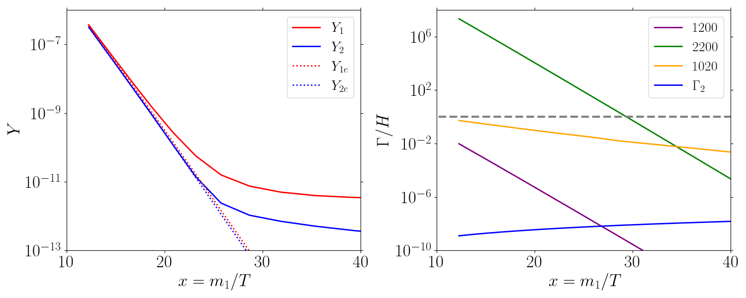
Deviations from the SBS will be explicitly shown in some parts of the paper. As a warm up example of the features of coscattering in the SBS, in Fig. 1 we show a typical evolution of the DM yield in the coscattering regime fulfilling the correct relic abundance , for GeV, and . Notice that deviates from its equilibrium already near , whereas stays in equilibrium for longer. This behavior is characteristic of the coscattering regime. In the right plot, we compare the reaction rates with the Hubble expansion, where and denotes the reaction density. In particular it can be seen that the DM conversion rate (yellow line) drops below the Hubble expansion at the same time as starts to freeze out from the thermal bath. Note that in the SBS scenario, decays and coannihilations are well below the Hubble rate and are completely negligible during the freeze-out process.
With this simple picture in mind, we now vary and and study their impact on the relic abundance. We have performed a grid scan over and GeV, keeping GeV and fixed. The results are shown in Fig. 2, where the red curves correspond to the solutions of the full cBE obtained with darkOmegaN, the blue curves where obtained using darkOmega and the orange curves where obtained ignoring the conversion processes . While the relic abundance shows a similar behavior when varying for different values of , the predicted relic abundance differs very strongly. This is due to the fact that the effective annihilation rate determining the point of freeze-out is exponentially suppressed for large . This suppression leads to a smaller effective cross section which implies a faster freeze-out and larger relic abundance, as can be seen in Fig. 2.
As an example to better understand the dependence of on , we consider the case GeV (dot-dashed line). In Fig. 2 we have highlighted three distinct regions for the behaviour of the relic abundance. The coscattering mechanism is only active in region I where is small enough so that the conversion processes freeze-out quickly. As the coupling increases, CE is recovered and the relic abundance becomes insensitive to in region II. In this case the relic abundance is mainly determined by annihilation, which is also called mediator freeze-out regime Junius:2019dci . Finally, in region III for coannihilations between and become relevant and the relic abundance again depends on .
For each in Fig. 2 we have also included the corresponding relic abundance obtained from darkOmegaN when neglecting the processes 1020, but keeping decays222In micrOMEGAs this is achieved using the option Excluding2010.. The resulting abundances are plotted as the orange lines, highlighting the fact that for small values of decays are not able to support CE in the absence of processes of the type 1020. In the case of on-shell decays (solid orange), where the decay rates are much larger, CE is maintained also at small . In this case the orange and red lines overlap in the whole range of small couplings.
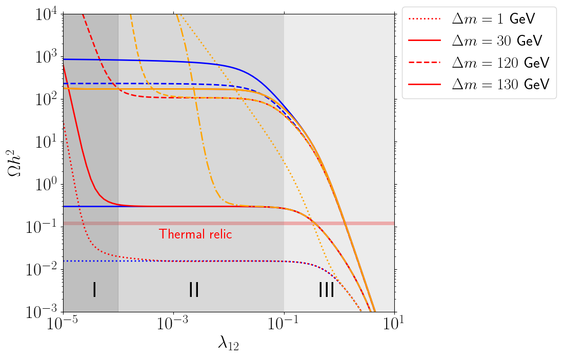
We have also included the results for the relic abundance calculated using the function darkOmega of micrOMEGAs (blue lines). This function assumes that that CE between and is maintained during the entire evolution of the DM yield. In case of and GeV, the relic abundance obtained with the functions darkOmega and darkOmegaN agree very well in regions II and III, indicating that CE is present. In case of GeV, the results assuming CE are larger by roughly a factor of two, which further increases for larger mass differences. We have checked that in these cases the rate of (inverse) decays remains above the Hubble expansion, ensuring CE. The correct relic abundance is therefore obtained from darkOmega, while darkOmegaN assumes separate CE of the different sectors, which is unrealistic, particularly when on-shell decays are present.
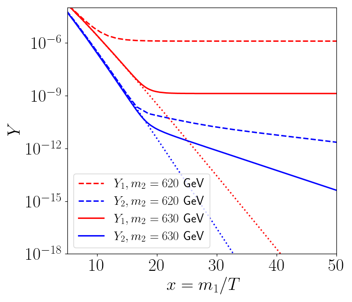
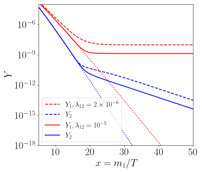
From the case with GeV shown in Fig. 2, we have seen that on-shell decays maintain CE for much smaller values. To further illustrate this fact, in Fig. 3 (left) we show the early departure from CE of the yield in the off-shell case, GeV, compared to the on-shell case, GeV, for a fixed value of . In Fig. 3 (right) we show that, once on-shell decays are present, small enough values of also break the CE333We have checked this in the case of on-shell decays, coscattering appears in the ballpark of , but as a strong overabundance is obtained in this parameter space region, we do not focus on this case in this paper.. In other words, as increases, the relevance of decays in maintaining CE becomes stronger, requiring smaller for coscattering.
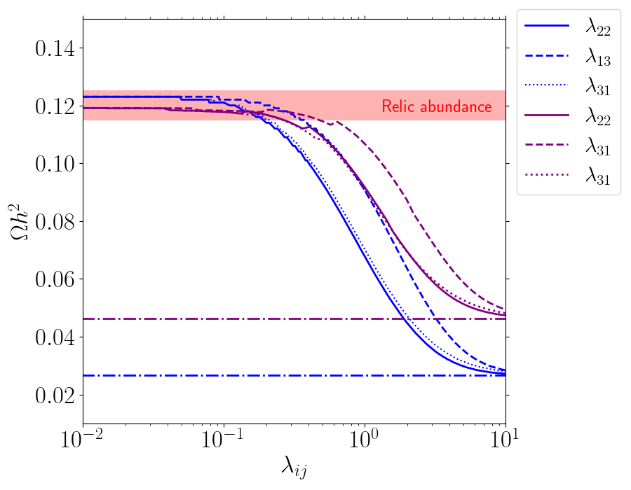
On the other hand, the contact terms proportional to the couplings and can have a strong impact on the relic density. In particular, when they take sizable values, i.e. either or , they bring and back into CE. To quantify this, in Fig. 4 (left) we show the effect of each separate coupling on the relic abundance for two set of masses. In each case, the value of was fixed in order to obtain the correct relic abundance by darkOmegaN in the limit of vanishing contact terms. As the contact couplings get sizable values, they start to affect the relic abundance calculation with darkOmegaN as they tend to establish partial CE between and . Once the contact couplings are big enough, the CE is established, such that the calculation using darkOmega and darkOmegaN agree with each other444It is interesting to remark that for the case in which takes sizable values, and remains sufficiently small to not maintain CE between and , one recover the yield dynamic of two stable DM, known as assisted freeze-out DiazSaez:2021pfw (also see Belanger:2011ww ; Maity:2019hre ). As in the present framework is unstable, after the breaking of its CE with , will continuously decrease as increases.. As we focus on the coscattering, we do not include deviations induced by the contact terms of this Higgs portal scenario, therefore in the rest of the paper we assume they are sufficiently small to not deviate from the relic abundance calculation with darkOmegaN.
To end this section, we comment about the low mass regime , which turns out to be disfavored by LHC data. From the above discussion we found that coscattering requires nearly degenerate masses of the new scalars, i.e. . On the other hand, we have checked numerically that in order to obtain the correct relic abundance would be large enough to also recover CE within the dark sector, making coscattering ineffective unless . However, searches of Higgs to invisible at the LHC have set limits on ATLAS:2022yvh , that translate into . We have also checked that the inclusion of the contact terms does not change this result.
To summarize, we have presented the cBE for the system of and , and we have solve them making use of the micrOMEGAs code. The three regimes that we have distinguished, coscattering, mediator FO, and (co)annihilations, depend strongly on the parameters and , with coscattering favoring and . Besides, on-shell (inverse) decay rates of are very efficient to maintain CE for much smaller values of than in the case of off-shell decays. Contact terms are not essential to have coscattering, and we have seen that light DM is ruled-out by LHC bounds.
4 Phenomenology
In this section we discuss direct detection and big-bang nucleosynthesis (BBN) constraints, and the prospects of having LLP in the coscattering scenario.
4.1 Constraints
4.1.1 Direct detection
The stable DM particle could be observed in direct detection experiments via the Higgs portal. This implies a bound on the effective DM-Higgs coupling Cline:2013gha
| (8) |
where denotes the upper bounds at 90% C.L on the effective DM-nucleon scattering cross section obtained from the LZ experiment LZ:2022lsv , the effective nucleon-Higgs coupling, GeV the nucleon mass, and GeV the SM Higgs mass.
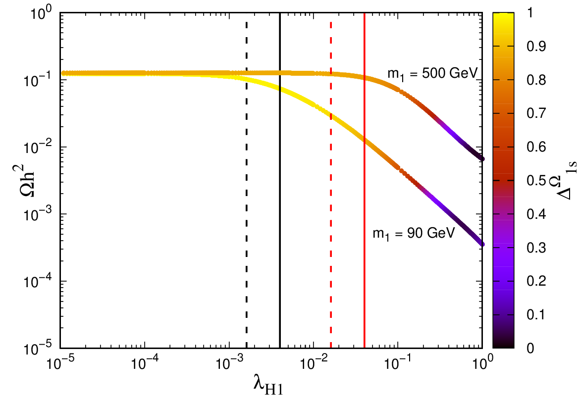
As coscattering can be achieved for sufficiently small values of , one could investigate the maximum values taken by this parameter without jeopardizing the relic abundance obtained by darkOmegaN at the same time being in the ballpark of those values that yield a strong enough signal to be searched in future direct detection experiments. Certainly, can not take arbitrarily large values, otherwise CE is recovered by processes of the type . To quantify the interplay among all these effects, in Fig. 4 we show the effect of on the relic abundance, for and GeV, GeV and . Besides, the color indicates the value of (see eq. 6). As expected, sizable values of decrease the relic abundance with respect to vanishing , and for very large values of this parameter CE is recovered. However, LZ bounds (solid vertical lines) do not allow such sizable values of , ruling out strong deviations from the co-scattering regime as given by darkOmegaN . In particular, for GeV, it is possible to have sizable values of this parameter, i.e. , in the ball park of LZ bounds (but still evading them), and without recovering CE. Actually, in that specific case, Darwin experiments DARWIN:2016hyl will be sensitive to regions with even smaller values of (dashed vertical lines in Fig. 4 (right)).
We point out that if loop corrections are considered, the DM-Higgs coupling should be renormalized on-shell in order to retain agreement with eq. (8) at higher orders. We have outlined a suitable treatment of loop corrections in appendix C and found that in our model the loop effects to the observables of interest are negligible.
4.1.2 BBN
Additional stable or decaying particles present at temperatures MeV may affect the measured primordial abundances of light elements. To our knowledge, constraints on lifetime of new singlet scalars have been only considered for masses Fradette:2017sdd . We estimate the bounds coming from BBN using the results obtained in Jedamzik:2006xz , considering the relic abundance of before its decay and the branching fraction of decays of into hadronic decays. In the present Higgs portal scenario, for GeV the model is practically safe of BBN constraints in the parameter space that we explore, since just after the decoupling of from the thermal plasma, is at least one order of magnitude below the measured DM relic abundance. The same conclusions were obtained in the leptophilic DM scenario in the coscattering mechanism Junius:2019dci .
4.2 Long-lived particles
In the coscattering regime, the coupling which determines the decay width of is very small, while simultaneously . Therefore, the dark partner typically constitutes a long-lived particle (LLP) with a wide range of possible lifetimes in different regions of the parameter space. While single production of (like production of the DM relic ) at colliders is suppressed by , pair production of through an intermediate Higgs boson must be sizable, via the chain Craig:2014lda
| (9) |
with being other states not relevant for the discussion. The goal of this section is to compare a few lifetime estimations predicted by the extended Higgs-singlet scenario that could be in the reach of present and future experiments, specially when the production mechanism is motivated by coscattering. In our knowledge, as LLP in Higgs portals have only been considered for mediator masses Curtin:2018mvb ; Alimena:2019zri , the results presented here could motivate the search of heavier scalars through the Higgs portal.
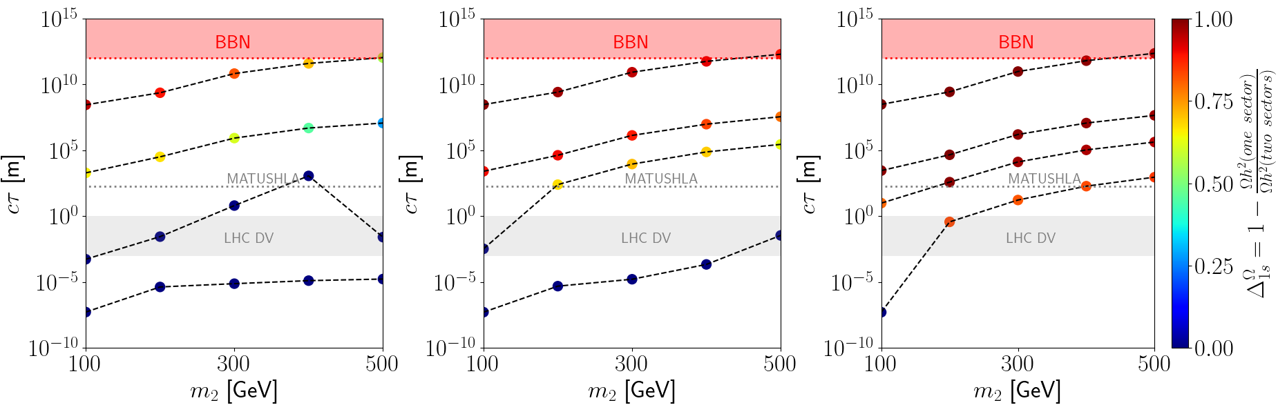
In Fig. 6, we show the results for the lifetime of as a function of its mass for and fixed (left), (middle) and (right). The row of points from top to bottom corresponds to 1, 5, 10 and 20 GeV, while the color of each point indicates . The variation in depends strongly on scalar mass difference, with small values of favoring the coscattering regime (), and in turn giving rise to enormous lifetimes of , with some of the points well beyond earth size experiments, thereby confronting bounds coming from BBN. As increases, the values of decrease to the point of reaching typical decay lengths for future experiments such as MATHUSLA Curtin:2018mvb . Notice that the reach of the latter may not only test particles that were produced in the coscattering regime, but also probe the other two regimes that we studied in Sec 3.2 (blue points). There are also model predictions in the reach of displaced vertex (DV) for ATLAS or CMS Lee:2018pag (grey band in each plot). Finally, the blue points in each plot are not unique for the corresponding chosen parameter space points shown in Fig. 6, since as some of them belong to the mediator freeze-out regime (see region II in Fig. 2), there is a range of values fulfilling the measured relic abundance, then varying in orders of magnitude their corresponding value.
5 Conclusions
In this work, we have studied for the very first time the simplest Higgs portal scenario in the context of coscattering. This SM extensions considers two real scalars charged under a single discrete symmetry, in which after EWSB, the lightest eigenstate is cosmologically stable, and the heavier one is unstable. We have explored in major detail the impact of each parameter in the thermal mechanism: coscattering, mediator freeze-out, and DM freeze-out. We put special attention to the first case, identifying parameter space for DM and mediator masses of hundreds of GeV giving the correct relic abundance. Radiative corrections do not generate significant deviations to the results that we obtain neither in direct detection nor in the calculation of the relic abundance. Besides, we have shown that the coscattering regime for the extended singlet-Higgs scenario gives rise to (very)long-lived mediators that could be in the reach of present and future experiments. Finally, effects of early kinetic decoupling Binder:2017rgn on the relic calculation could modify at some extent the results presented in this work, but this analysis is beyond the scope of our work.
Acknowledgements.
We thank the creators and developers of micrOMEGAs, and a special thank to Sasha Pukhov for his constant assistance on micrOMEGAs. We thank Gael Alguero for providing important information relevant to our work. We also thank Giovanna Cottin for helpful advice on the long-lived particle subject. B.D.S has been founded by ANID (ex CONICYT) Grant No. 3220566. B.D.S. and J.L want to thank DESY and the Cluster of Excellence Quantum Universe, Hamburg, Germany, were this work was initiated.Appendix A Lagrangian original basis
In this appendix we develop the details of the model in terms of the original field basis, which after some algebra becomes the simplified Lagrangian that we used in eq. 1.
Let us consider two real singlet scalars and , charged under the same symmetry such that and , with Casas:2017jjg ; Ghorbani:2014gka . The corresponding potential is given by
| (10) | |||||
After EWSB, with , the scalars and mix, but after rotation the potential can be written identically as in 10. We diagonalize using
| (11) |
The mass matrix is
| (12) |
The Eigenmass are given by
| (13) | |||||
| (14) |
Additionally, from the non-diagonal relationship of eq. 11 we obtain that
| (15) |
Replacing eq. 15 into the original Lagrangian, and writing down eq. 10 in terms of the physical states, i.e. and , we obtain the potential presented in eq. 1.
Appendix B Dark Matter Conversion Rate
In this section we present a calculation of the thermally averaged cross section for DM conversion where can be any SM particle. The differential cross section of the conversion process in the centre of mass frame is given by
| (16) |
where denotes the total c.o.m. energy, denotes the final state momentum555 is the Källén function. and and denote the energies of the initial state DM and SM particle with momentum . At tree-level the conversion processes are possible for through the -channel diagrams shown in Fig. 7. The resulting squared matrix elements are given by
| (17a) | ||||
| (17b) | ||||
| (17c) | ||||
where
| (18) |
After substitution, the solid angle differential becomes and the integrals can be solved to obtain the total cross section
| (19a) | ||||
| (19b) | ||||
| (19c) | ||||
where . Next, the thermal average has to be calculated from
| (20) |
To good approximation, this integral is given by where
| (21) |
such that the thermally averaged cross sections, in the limit , are given by
| (22a) | ||||
| (22b) | ||||
| (22c) | ||||
Finally, the DM conversion rate is .
Appendix C Treatment of Radiative Corrections
In this appendix we outline the on-shell renormalization of the model and estimate the impact of one-loop corrections on the results obtained in this paper. We note that a proper definition of the renormalization conditions is crucial in order to obtain meaningful results at NLO. In particular, the physical interpretation of the parameters at tree-level is only retained if they fulfill corresponding on-shell renormalization conditions at one-loop order. In other schemes like or for ad-hock subtractions the model parameters no longer correspond directly to the observables of interest. The parameters relevant for a renormalization of the scalar sector are the scalar masses , quartic couplings and Higgs vev . The renormalized Lagrangian is obtained from the following renormalization transformation of the bare parameters
| (23) |
and renormalization of the bare fields
| (24) |
After on-shell renormalization, the scalar masses correspond to the physical pole masses of the DM particles and the scalar couplings correspond to physical effective coupling strengths measured e.g. in direct detection or collision experiments. This implies a set of conditions on the corresponding amplitudes from which the renormalization constants can be determined. Here, we demonstrate this specifically for and , which where chosen to be very small in the above analysis. We define to be the effective -Higgs coupling measured in the direct detection experiments sketched in Fig. 8 (left), while is defined through DM production and annihilation events at such as in Fig. 8 (right). Note that, in general, the effective (quantum corrected) DM-Higgs couplings denoted by will be dependent on the (off-shell) Higgs momentum . At one-loop these effective couplings are given by
| (25a) | ||||
| (25b) | ||||
where denotes the contributions of the one-loop diagrams from Fig. 9. The definitions of the coupling strenghts translate into the following renormalization conditions
| (26) |
And can easily be fulfilled by choosing the renormalization constants and appropriately. In the limit the only contributing one-loop diagrams are of the type Fig. 9 (left) and result in the following expressions for the renormalized vertex functions
| (27) | ||||
| (28) |
By definition of the on-shell scheme, quantum corrections to direct detection of and to annihilation and production processes of during freeze-out are 0. Corrections only appear for annihilation and production of , where the relevant momentum transfer is . The resulting effective coupling that should be used when calculating the relic abundance is (for )
| (29) |
The loop corrections, as expected, result in very small effects and do not have any important impact on the above analysis.
References
- (1) R.T. D’Agnolo, D. Pappadopulo and J.T. Ruderman, Fourth Exception in the Calculation of Relic Abundances, Phys. Rev. Lett. 119 (2017) 061102 [1705.08450].
- (2) M. Garny, J. Heisig, B. Lülf and S. Vogl, Coannihilation without chemical equilibrium, Phys. Rev. D 96 (2017) 103521 [1705.09292].
- (3) H.-C. Cheng, L. Li and R. Zheng, Coscattering/Coannihilation Dark Matter in a Fraternal Twin Higgs Model, JHEP 09 (2018) 098 [1805.12139].
- (4) M. Garny, J. Heisig, M. Hufnagel and B. Lülf, Top-philic dark matter within and beyond the WIMP paradigm, Phys. Rev. D 97 (2018) 075002 [1802.00814].
- (5) R.T. D’Agnolo, C. Mondino, J.T. Ruderman and P.-J. Wang, Exponentially Light Dark Matter from Coannihilation, JHEP 08 (2018) 079 [1803.02901].
- (6) F. Brümmer, Coscattering in next-to-minimal dark matter and split supersymmetry, JHEP 01 (2020) 113 [1910.01549].
- (7) S. Junius, L. Lopez-Honorez and A. Mariotti, A feeble window on leptophilic dark matter, JHEP 07 (2019) 136 [1904.07513].
- (8) R.T. D’Agnolo, D. Pappadopulo, J.T. Ruderman and P.-J. Wang, Thermal Relic Targets with Exponentially Small Couplings, Phys. Rev. Lett. 124 (2020) 151801 [1906.09269].
- (9) M. Garny and J. Heisig, Bound-state effects on dark matter coannihilation: Pushing the boundaries of conversion-driven freeze-out, Phys. Rev. D 105 (2022) 055004 [2112.01499].
- (10) J. Herms and A. Ibarra, Production and signatures of multi-flavour dark matter scenarios with t-channel mediators, JCAP 10 (2021) 026 [2103.10392].
- (11) J. Heeck, J. Heisig and A. Thapa, Dark matter and radiative neutrino masses in conversion-driven scotogenesis, Phys. Rev. D 107 (2023) 015028 [2211.13013].
- (12) A. Filimonova, S. Junius, L. Lopez Honorez and S. Westhoff, Inelastic Dirac dark matter, JHEP 06 (2022) 048 [2201.08409].
- (13) J. Heisig, A. Lessa and L.M.D. Ramos, Probing conversion-driven freeze-out at the LHC, 2404.16086.
- (14) D. Curtin et al., Long-Lived Particles at the Energy Frontier: The MATHUSLA Physics Case, Rept. Prog. Phys. 82 (2019) 116201 [1806.07396].
- (15) G. Cottin, LLP overview: theory perspective, PoS LHCP2023 (2024) 164.
- (16) K. Ghorbani and H. Ghorbani, Scalar split WIMPs in future direct detection experiments, Phys. Rev. D93 (2016) 055012 [1501.00206].
- (17) J.A. Casas, D.G. Cerdeño, J.M. Moreno and J. Quilis, Reopening the Higgs portal for singlet scalar dark matter, JHEP 05 (2017) 036 [1701.08134].
- (18) G. Belanger, F. Boudjema, A. Pukhov and A. Semenov, MicrOMEGAs: A Program for calculating the relic density in the MSSM, Comput. Phys. Commun. 149 (2002) 103 [hep-ph/0112278].
- (19) G. Alguero, G. Belanger, S. Kraml and A. Pukhov, Co-scattering in micrOMEGAs: a case study for the singlet-triplet dark matter model, 2207.10536.
- (20) B. Díaz Sáez, K. Möhling and D. Stöckinger, Two real scalar WIMP model in the assisted freeze-out scenario, JCAP 10 (2021) 027 [2103.17064].
- (21) G. Belanger and J.-C. Park, Assisted freeze-out, JCAP 1203 (2012) 038 [1112.4491].
- (22) T.N. Maity and T.S. Ray, Exchange driven freeze out of dark matter, Phys. Rev. D 101 (2020) 103013 [1908.10343].
- (23) ATLAS collaboration, Search for invisible Higgs-boson decays in events with vector-boson fusion signatures using 139 fb-1 of proton-proton data recorded by the ATLAS experiment, JHEP 08 (2022) 104 [2202.07953].
- (24) J.M. Cline, K. Kainulainen, P. Scott and C. Weniger, Update on scalar singlet dark matter, Phys. Rev. D 88 (2013) 055025 [1306.4710].
- (25) LZ collaboration, First Dark Matter Search Results from the LUX-ZEPLIN (LZ) Experiment, Phys. Rev. Lett. 131 (2023) 041002 [2207.03764].
- (26) DARWIN collaboration, DARWIN: towards the ultimate dark matter detector, JCAP 11 (2016) 017 [1606.07001].
- (27) A. Fradette and M. Pospelov, BBN for the LHC: constraints on lifetimes of the Higgs portal scalars, Phys. Rev. D 96 (2017) 075033 [1706.01920].
- (28) K. Jedamzik, Big bang nucleosynthesis constraints on hadronically and electromagnetically decaying relic neutral particles, Phys. Rev. D 74 (2006) 103509 [hep-ph/0604251].
- (29) N. Craig, H.K. Lou, M. McCullough and A. Thalapillil, The Higgs Portal Above Threshold, JHEP 02 (2016) 127 [1412.0258].
- (30) J. Alimena et al., Searching for long-lived particles beyond the Standard Model at the Large Hadron Collider, J. Phys. G 47 (2020) 090501 [1903.04497].
- (31) L. Lee, C. Ohm, A. Soffer and T.-T. Yu, Collider Searches for Long-Lived Particles Beyond the Standard Model, Prog. Part. Nucl. Phys. 106 (2019) 210 [1810.12602].
- (32) T. Binder, T. Bringmann, M. Gustafsson and A. Hryczuk, Early kinetic decoupling of dark matter: when the standard way of calculating the thermal relic density fails, Phys. Rev. D 96 (2017) 115010 [1706.07433].