This paper was converted on www.awesomepapers.org from LaTeX by an anonymous user.
Want to know more? Visit the Converter page.

Cosmic Accelerations Characterize the Instability of the Critical Friedmann Spacetime

[Uncaptioned image] Christopher Alexander
Department of Mathematics
University College London
London, WC1H 0AY
United Kingdom
christopher.alexander@ucl.ac.uk
&[Uncaptioned image] Blake Temple
Department of Mathematics
University of California
Davis, CA 95616
United States
temple@math.ucdavis.edu
&Zeke Vogler
Department of Mathematics
University of California
Davis, CA 95616
United States
zekius@math.ucdavis.edu
Abstract

We give a definitive characterization of the instability of the pressureless (p=0p=0) critical (k=0k=0) Friedmann spacetime to smooth radial perturbations. We use this to characterize the global accelerations away from k0k\leq 0 Friedmann spacetimes induced by the instability in the underdense case. The analysis begins by incorporating the Friedmann spacetimes into a mathematical analysis of smooth spherically symmetric solutions of the Einstein field equations expressed in self-similar coordinates (t,ξ)(t,\xi) with ξ=rt<1\xi=\frac{r}{t}<1, conceived to realize the critical Friedmann spacetime as an unstable saddle rest point SMSM. We identify a new maximal asymptotically stable family \mathcal{F} of smooth outwardly expanding solutions which globally characterize the evolution of underdense perturbations. Solutions in \mathcal{F} align with a k<0k<0 Friedmann spacetime at early times, generically introduce accelerations away from k<0k<0 Friedmann spacetimes at intermediate times and then decay back to the same k<0k<0 Friedmann spacetime as tt\to\infty uniformly at each fixed radius r>0r>0. We propose \mathcal{F} as the maximal asymptotically stable family of solutions into which generic underdense perturbations of the unstable critical Friedmann spacetime will evolve and naturally admit accelerations away from Friedmann spacetimes within the dynamics of solutions of Einstein’s original field equations, that is, without recourse to a cosmological constant or dark energy.

Keywords General Relativity  \cdot Instability  \cdot Cosmology  \cdot Dark Energy

This material is based upon work supported by EPSRC Project: EP/S02218X/1

1 Introduction

In our 2017 announcement in Proceedings of the Royal Society A [29],111Authors dedicate this paper to our former collaborator and long-time friend Joel Smoller and acknowledge our use of unpublished notes which were the basis for [29] and represent the point of departure for the present paper. Smoller, Temple and Vogler introduced the STV-PDE, a version of the perfect fluid Einstein field equations for spherically symmetric spacetimes. These were obtained by starting with the spacetime metric in standard Schwarzschild coordinates (SSC) and then re-expressing it using the self-similar variable ξ=rt\xi=\frac{r}{t} in place of rr, assuming zero cosmological constant and assuming |ξ|<1|\xi|<1 to keep ξ\xi as a spacelike coordinate. Since ξ=1\xi=1 is a measure of the distance of light travel since the Big Bang in a Friedmann spacetime,222By a Friedmann spacetime, we mean a Friedmann–Lemaître–Robertson–Walker (FLRW) spacetime. Also recall that the curvature parameter kk in Friedmann spacetimes can always be scaled to one of the values k=1,0,1k=-1,0,1. The k=0k=0 spacetime is unique and k=±1k=\pm 1 spacetimes each describe a one parameter family of distinct spacetimes depending on the single parameter Δ0\Delta_{0} defined below in (5.17). Thus we refer to k<0k<0 Friedmann spacetimes by kk or Δ0\Delta_{0}. Unless a different equation of state is specified, our use of the term Friedmann always assumes a dust (p=0p=0) solution of the Einstein field equations. we view |ξ|<1|\xi|<1 as valid out to approximately the Hubble radius, a measure of the distance across the visible Universe [31]. The STV-PDE were conceived to represent the pressureless (p=0p=0) critical (k=0k=0) Friedmann spacetime as an unstable saddle rest point333We refer to a rest point of a PDE as a time independent solution depending only on ξ\xi. The character of a rest point of the STV-PDE, that is, unstable, stable and so on, is determined by the character it exhibits in the approximating STV-ODE obtained by the expansion of solutions in powers of ξ\xi, as described later., which we denote by SMSM for Standard Model. This is based on the important realization that the metric components and fluid variables of the p=0p=0, k=0k=0 Friedmann spacetime in SSC can be expressed as a function of ξ\xi alone in an appropriate time gauge (see [29] and Theorem 30 below). The character of a rest point is difficult to disentangle in coordinate systems, such as comoving coordinates, where it appears time dependent, especially so for PDE. To analyze rest points of PDE requires a procedure of finite approximation and this was manifested in [29] by the observation that solutions of the STV-PDE which are smooth at the center of symmetry can be developed into a regular expansion in even powers of ξ\xi with time dependent coefficients. This generates a nested sequence of autonomous 2n×2n2n\times 2n ODE which close444This asymptotic expansion does not close at order nn when p0p\neq 0 [29]. in the time dependent coefficients at every order n1n\geq 1. We name the resulting 2n×2n2n\times 2n system of ODE the STV-ODE of order nn and observe that at each order, the STV-ODE is autonomous in the log-time variable τ=lnt\tau=\ln t (so 0<t<0<t<\infty and <τ<-\infty<\tau<\infty). Moreover, the phase portrait of the resulting autonomous system at each order contains the unstable saddle rest point SMSM, together with the stable degenerate rest point MM. MM, for Minkowski, is the limit of the time asymptotic decay of solutions as tt\to\infty.555The presence of a single rest point MM which characterizes the late time dynamics of solutions is a serendipitous simplification inherent in the choice of self-similar coordinates.

The STV-ODE are nested in the sense that higher order solutions provide strict refinements of solutions determined at lower orders. We prove that the STV-ODE are linear inhomogeneous ODE at every order n>1n>1 in the sense that the coefficients of the highest order terms are always of lower order. Our analysis shows that the eigenvalue structure of the rest points SMSM and MM determine the character of the phase portrait of the STV-ODE at every order and the essential character of all the phase portraits can be deduced from the phase portraits at orders n=1n=1 and n=2n=2. Our analysis establishes that k<0k<0 and k>0k>0 Friedmann spacetimes correspond to unique solution trajectories which lie in the unstable manifold of SMSM at all orders of the STV-ODE, and general higher order solutions of the STV-ODE agree exactly with a Friedmann spacetime at order n=1n=1. In particular, we prove that the phase portraits of the STV-ODE of order n=1n=1 and n=2n=2 characterize the instability of k0k\leq 0 Friedmann spacetimes: The k=0k=0 Friedmann spacetime is unstable with a codimension one unstable manifold, while the k<0k<0 Friedmann spacetimes are locally unstable at SMSM but are globally asymptotically stable in the sense that all underdense perturbations of SMSM tend to the same rest point MM as tt\to\infty. Moreover, this remains true at all orders n>2n>2 and a smooth solution of the STV-PDE will lie in the unstable manifold of SMSM at all orders n1n\geq 1 of the STV-ODE if and only if it lies in the unstable manifold of SMSM at order n=2n=2.

The existence of a second positive eigenvalue of SMSM at order n=2n=2 (the first being at order n=1n=1) implies the existence of a one parameter family of nontrivial solutions of the STV-ODE of order n=2n=2 which exist within the unstable manifold of SMSM but diverge from Friedmann spacetimes at that order. The existence of a second negative eigenvalue at SMSM at order n=2n=2 establishes that the unstable manifold of SMSM is a codimension one space of trajectories, so solutions of the STV-ODE are generically not within the unstable manifold of SMSM. We prove that at order n=2n=2 all solutions in the unstable manifold of SMSM exit tangent to the trajectory associated with Friedmann spacetimes but a unique positive eigenvalue smaller than the leading order eigenvalue enters at order n=3n=3. Since the eigenvector associated with the smallest eigenvalue dominates at rest point SMSM in backward time, it follows that generic solutions in the unstable manifold of SMSM exit tangent to a new eigendirection, different from Friedmann, at all orders n=3n=3 and above.

The stable and unstable manifolds of SMSM together with the stable manifold of MM characterize the global phase portraits of the STV-ODE at all orders. An analysis of the phase portraits lead to the introduction of a new family \mathcal{F} of solutions of the STV-PDE that extend the k<0k<0 Friedmann spacetimes to a maximal asymptotically stable family of solutions into which underdense perturbations of the unstable k=0k=0 Friedmann spacetime will globally evolve and generically accelerate away from Friedmann spacetimes early on. Thus \mathcal{F} globally characterizes the instability of the p=0p=0, k=0k=0 Friedmann spacetime to smooth radial underdense perturbations. We prove that solutions in \mathcal{F} align with a k<0k<0 Friedmann spacetime at early times, introduce accelerations away from k<0k<0 Friedmann spacetimes at intermediate times and then decay back to the same k<0k<0 Friedmann spacetime as tt\to\infty (at each fixed r>0r>0). The existence of positive eigenvalues at SMSM, with eigensolutions tending to MM as tt\to\infty at every order n1n\geq 1 of the STV-ODE, demonstrates the global instability of the k=0k=0 Friedmann spacetime to perturbation at every order. On the other hand, the decay of solutions in \mathcal{F} to the rest point MM as tt\to\infty establishes the global large time asymptotic stability of all k<0k<0 Friedmann spacetimes. However, the existence of a second positive eigenvalue at SMSM at order n=2n=2 demonstrates the instability of k<0k<0 Friedmann spacetimes to perturbation within the unstable manifold of SMSM at early times, implying that solutions in \mathcal{F} generically accelerate away from Friedmann spacetimes at intermediate times before asymptotic stability brings them back to a k<0k<0 Friedmann spacetime via decay to MM as tt\to\infty (for fixed r>0r>0). The existence of positive eigenvalues of SMSM at every order implies that a similar instability of k<0k<0 Friedmann spacetimes occurs at t=0t=0 within the unstable manifold of SMSM at every order n3n\geq 3 of the STV-ODE as well. We conclude that solutions in \mathcal{F} characterize both the instability of the p=0p=0, k=0k=0 Friedmann spacetime to smooth radial underdense perturbations and characterize the accelerations away from Friedmann spacetimes at intermediate times, both within the dynamics of Einstein’s original field equations, that is, without recourse to a cosmological constant or dark energy.

1.1 Introduction to the Family of Spacetimes \mathcal{F}

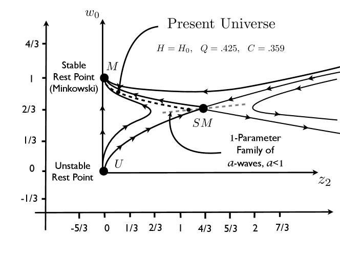
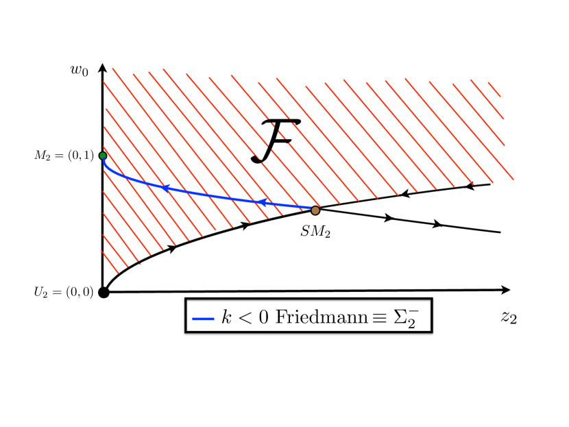
We argued in [29] that solutions of the p=0p=0 STV-PDE which are smooth at the center of symmetry can be expanded in even powers of ξ\xi by Taylor’s theorem (see Section 3) and from the nthn^{th} order term we obtain an approximation which solves the STV-ODE of order nn. In the present paper we go on to prove that, for each such solution, there exists a solution dependent time translation tttt\to t-t_{*} of the SSC time coordinate tt, which we call time since the Big Bang, such that making the SSC gauge transformation to time since the Big Bang has the effect of eliminating the leading order negative eigenvalue at SMSM. Moreover, this gauge transforms every solution to either the rest point SMSM or one of the two trajectories in the unstable manifold of SMSM at n=1n=1. As a result of this, every solution agrees exactly with a k<0k<0, k=0k=0 or k>0k>0 Friedmann spacetime in the phase portrait of the STV-ODE at leading order n=1n=1, see Figure 1. There is an important distinction to make here: The STV-ODE are autonomous in log-time τ=lnt\tau=\ln t, so translation in τ\tau maps solutions to physically different solutions which traverse the same trajectory of the STV-ODE, but translation in tt is a gauge freedom of the SSC metric ansatz which maps trajectories of the STV-ODE to different trajectories which represent the same physical solution. Thus choosing time since the Big Bang eliminates a physical redundancy in the solution trajectories of the STV-ODE. When time since the Big Bang is imposed, there are only three remaining trajectories in the leading order n=1n=1 phase portrait of the STV-ODE: The unstable rest point SMSM, the underdense (left) component of the unstable manifold and the overdense (right) component of the unstable manifold, see Figure 1. The underdense component of the unstable manifold of SMSM at n=1n=1 is the unique trajectory which takes SMSM to MM and corresponds to k<0k<0 Friedmann spacetimes, with the value of kk determined by translation in τ\tau along this unique trajectory. The unique trajectory exiting SMSM in the opposite overdense direction is the component of the unstable manifold of SMSM corresponding to k>0k>0 Friedmann spacetimes. The three (including the fixed point SMSM) trajectories of the n=1n=1 phase portrait, after time since the Big Bang is imposed, is diagrammed in Figure 2.

In this paper we identify and study the entire subset of solutions \mathcal{F} of the STV-PDE defined by the condition that, when time tt is taken to be time since the Big Bang, the resulting solution agrees with an underdense k<0k<0 Friedmann solution in the leading order n=1n=1 STV-ODE phase portrait. That is, the solution projects to the unique trajectory in the unstable manifold of SMSM which takes SMSM to MM at order n=1n=1, parameterized by ττ0\tau-\tau_{0} for some log-time translation constant τ0=lnt0\tau_{0}=\ln t_{0} of the autonomous STV-ODE. We identify \mathcal{F} as a new maximal asymptotically stable family of outwardly expanding solutions of the STV-PDE defined by the condition that solutions agree with a k<0k<0 Friedmann spacetime in the leading order phase portrait of the expansion in even powers of ξ\xi when the SSC time is translated to time since the Big Bang associated with each solution. The main purpose of this paper is to demonstrate and characterize the instability of the k=0k=0 Friedmann spacetime and the large time asymptotic stability and early time instability of the k<0k<0 Friedmann spacetimes within the family of solutions \mathcal{F}.

We first characterize the forward time dynamics and asymptotic stability of solutions in \mathcal{F} by proving that every solution which decays to the rest point MM as tt\to\infty in the phase portrait of the STV-ODE at order n=1n=1, that is, every solution in \mathcal{F}, also decays as tt\to\infty to a corresponding unique stable rest point MM in the phase portrait of the STV-ODE at every order n1n\geq 1. This characterizes the forward time dynamics of solutions in \mathcal{F} because it implies that every solution in \mathcal{F} decays, as tt\to\infty, to a k<0k<0 Friedmann spacetime faster than it decays to Minkowski space as tt\to\infty at each fixed radii r>0r>0 at every order n1n\geq 1. The asymptotic decay of solutions in \mathcal{F} as tt\to\infty immediately implies uniform bounds on solutions of the STV-ODE for all time t>t0>0t>t_{0}>0 and n1n\geq 1 in terms of bounds on the initial data at t=t0>0t=t_{0}>0 alone. The STV-ODE are linear in the highest order variables when lower order solutions are interpreted as known inhomogeneous terms, so solutions of the STV-ODE exist for all time 0<t<0<t<\infty at every order. For the purposes of asymptotic analysis, we formally assume convergence of solutions of the STV-ODE up to order nn, with errors at order nn estimated by bounds at order n+1n+1 according to Taylor’s theorem, an assumption justified rigorously by simply restricting to an appropriate space of analytic solutions.666The convergence of solutions in \mathcal{F} in the limit nn\to\infty for |ξ|<1|\xi|<1, with estimates provided by Taylor’s theorem, follows directly from mild assumptions on the growth rate of the initial data, due to the fact that all solutions lie on bounded trajectories which tend to MM as tt\to\infty at every order n1n\geq 1.

The backward time dynamics t0t\to 0 (τ\tau\to-\infty) of solutions in \mathcal{F} is determined at each order n1n\geq 1 by the instability of the k=0k=0 Friedmann spacetime, that is, by the eigenvalues of the saddle rest point SMSM as it is represented in the STV-ODE phase portrait at each order n1n\geq 1. By definition, each solution in \mathcal{F} agrees at leading order (n=1n=1) with a k<0k<0 Friedmann spacetime represented as the unique trajectory in the unstable manifold of SMSM which tends to MM as tt\to\infty and to SMSM as t0t\to 0. To understand the backward time dynamics of solutions in \mathcal{F} at higher orders n2n\geq 2, we demonstrate that k<0k<0 Friedmann solutions correspond to a single trajectory in the unstable manifold of SMSM in the phase portrait of the STV-ODE at every order n1n\geq 1, with the value of kk determined by log-time translation at order n=1n=1. We then prove that two new eigenvalues of the rest point SMSM appear at each new order n2n\geq 2 and all of them are positive except one negative eigenvalue which appears at order n=2n=2. From this we conclude that the family \mathcal{F} decomposes into two essential components: The underdense component of the unstable manifold of SMSM, consisting of trajectories which connect SMSM to MM at every order n1n\geq 1, and solutions which tend to MM in forward time but do not tend to SMSM in backwards time. Because of the presence of the order n=2n=2 negative eigenvalue at SMSM, solutions in \mathcal{F} will generically not tend to SMSM in backward time, but rather will follow the one-dimensional stable manifold of SMSM, the unique trajectory which emerges from SMSM in backward time as t0t\to 0 (τ\tau\to-\infty). Thus the Big Bang limit t0t\to 0 of a generic solution in \mathcal{F} is not self-similar like SMSM beyond the leading order, but rather, generically displays a non-self-similar character at the Big Bang for all orders n=2n=2 and above. This provides an important example of the self-similarity hypothesis, that solutions which approach a singularity exhibit self-similarity to leading order [4]. However, in this case, such solutions are generically not self-similar beyond leading order.

To reiterate, each spacetime in \mathcal{F} agrees with a unique k<0k<0 Friedmann spacetime in the phase portrait of the STV-ODE at leading order n=1n=1 (all the way into the Big Bang at t=0t=0) and agrees with the same k<0k<0 Friedmann spacetime in the limit tt\to\infty (for each fixed r>0r>0), but generically accelerates away from this k<0k<0 Friedmann spacetime at intermediate times in the phase portraits of the STV-ODE of order n2n\geq 2. Since each member of the family \mathcal{F} by definition contains the component of the unstable manifold of SMSM which contains the leading order behavior of k<0k<0 Friedmann spacetimes imposed at n=1n=1, \mathcal{F} represents a maximal extension of the one parameter family of k<0k<0 Friedmann spacetimes to a robust asymptotically stable family of spacetimes which exist within the family of smooth spherically symmetric spacetimes. Since the family \mathcal{F} is the full space of solutions into which underdense perturbations of SMSM evolve, \mathcal{F} characterizes the instability of SMSM to underdense perturbations. Because a negative eigenvalue of SMSM does not exist above order n=2n=2, it follows that a solution in \mathcal{F} lies in the unstable manifold of SMSM if and only if its projection onto the n=2n=2 phase portrait of the STV-ODE lies in the unstable manifold of SMSM, so the unstable manifold of SMSM at n=2n=2 characterizes the unstable manifold of SMSM at all orders. A main goal of this paper is to prove that, even though \mathcal{F} is asymptotically stable, solutions in \mathcal{F} generically accelerate away from k<0k<0 Friedmann spacetimes at early times due to an instability at t=0t=0.

To establish the instability of k<0k<0 Friedmann spacetimes at t=0t=0, it suffices to demonstrate that there are multiple solutions of the STVODESTV-ODE which agree with k<0k<0 Friedmann spacetimes at order n=1n=1 and in the limit t0t\to 0 but which diverge from k<0k<0 Friedmann spacetimes at t>0t>0 for some n2n\geq 2. Imposing time since the Big Bang, every solution in \mathcal{F} lies on the unique trajectory in the unstable manifold of SMSM which takes SMSM to MM and hence every solution agrees with a k<0k<0 Friedmann solution at order n=1n=1. Thus to establish the instability of k<0k<0 Friedmann spacetimes at order n=2n=2, it suffices to prove that: (1) Solution trajectories corresponding to k<0k<0 Friedmann lie in the unstable manifold of SMSM and (2) there exist other solutions in \mathcal{F} in the unstable manifold of SMSM which diverge from k<0k<0 Friedmann at t>0t>0. For this, we use known exact formulas to prove that the solution trajectory of k<0k<0 Friedmann spacetimes lies in the unstable manifold of SMSM at order n=2n=2 with time translation differentiating kk. Since a solution in \mathcal{F} lies in the unstable manifold of SMSM at every order if and only if it lies in the unstable manifold of SMSM order n=2n=2, we can conclude that k<0k<0 Friedmann spacetimes lie on a single trajectory in the unstable manifold of SMSM at every order n2n\geq 2 as well. Next we use exact formulas to prove that the trajectory corresponding to k<0k<0 Friedmann spacetimes at order n=2n=2 is an eigensolution of the eigenvalue λA1\lambda_{A1} which enters at order n=1n=1 (this is also shown to order n=3n=3 in Section 12). Thus to establish the instability of k<0k<0 Friedmann spacetimes it suffices only to prove that a second positive eigenvalue λB2λA1\lambda_{B2}\neq\lambda_{A1} emerges at SMSM at order n=2n=2. From this, the early time instability of the k<0k<0 Friedmann spacetimes is established in the phase portrait of the STV-ODE of order n=2n=2, diagrammed in Figure 3, even though the whole family \mathcal{F} is asymptotically stable. We discuss the phase portrait at order n=2n=2 in Section 1.6.

At this stage it is convenient to introduce a refined notation that distinguishes the family \mathcal{F} of solutions of the STV-PDE from the solutions of the STV-ODE which approximate solutions in \mathcal{F} up to arbitrary order. To this end, we define n\mathcal{F}_{n} as the set of solutions of the STV-ODE of order nn which satisfy the property that the trajectory reduces at order n=1n=1 to the unique trajectory which connects SMSM to MM, but not necessarily at higher orders. We also define nn\mathcal{F}_{n}^{\prime}\subset\mathcal{F}_{n} to be the subset of solutions which lie in the unstable manifold of the rest point SMSM in STV-ODE of order nn. Note that by definition 1=1\mathcal{F}_{1}^{\prime}=\mathcal{F}_{1}. Finally, let \mathcal{F}^{\prime}\subset\mathcal{F} denote the set of solutions of the STV-PDE whose nthn^{th} order approximation lies in the unstable manifold of rest point SMSM in the phase portrait of the STV-ODE of order nn for every n1n\geq 1. We may sometimes refer to n\mathcal{F}_{n} as \mathcal{F} at order nn and n\mathcal{F}_{n}^{\prime} as the stable manifold of SMSM in \mathcal{F} at order nn.

Having set out the main elements, we now discuss them in detail.

1.2 The STV-PDE

In Section 7 we give a new derivation of the Einstein field equations G=κTG=\kappa T in what we call SSCNG coordinates. These coordinates are standard Schwarzschild coordinates (SSC), that is, where the metric takes the form

ds2=B(t,r)dt2+dr2A(t,r)+r2dΩ2,\displaystyle ds^{2}=-B(t,r)dt^{2}+\frac{dr^{2}}{A(t,r)}+r^{2}d\Omega^{2}, (1.1)

in addition to possessing a normal gauge (NG) when expressed in the variables (t,ξ)(t,\xi). An arbitrary spherically symmetric spacetime can generically777That is, under the condition C(t,r)r0\frac{\partial C(t,r)}{\partial r}\neq 0, where C(t,r)dΩ2C(t,r)d\Omega^{2} is the angular part of the metric, see [29]. be transformed to SSC metric form by defining rr so r2dΩ2r^{2}d\Omega^{2} is the angular part of the metric and then constructing a time coordinate tt, complementary to rr, such that the metric is diagonal in (t,r)(t,r)-coordinates [31, 34]. The SSC metric form is invariant under the gauge freedom of arbitrary time transformation tϕ(t)t\to\phi(t), so to set the gauge, we impose the condition that B(t,0)=1B(t,0)=1, that is, geodesic (proper) time at r=0r=0 [29]. We refer to this as the normal gauge (NG).

The STV-PDE use density and velocity variables:

z\displaystyle z =κρr21v2,\displaystyle=\frac{\kappa\rho r^{2}}{1-v^{2}}, w\displaystyle w =vξ,\displaystyle=\frac{v}{\xi},

coupled to the SSC metric components AA and D=ABD=\sqrt{AB}. Recall that the STV-PDE are not the Einstein field equations in (t,ξ)(t,\xi) coordinates but rather the Einstein field equations with an SSC metric form expressed in terms of zz and ww with independent variables (t,ξ)(t,\xi) [29]. We extend the derivation of the STV-PDE to equations of state of the form p=σρp=\sigma\rho, with σ\sigma constant, in Theorem 32 below. However, our concern in this paper is with the case p=σ=0p=\sigma=0, applicable to late time Big Bang Cosmology.888In the Standard Model of Cosmology, the pressure drops precipitously to zero at about 10,000 years after the Big Bang, an order of magnitude before the uncoupling of matter and radiation [17].

Theorem 1 (Special case of Theorem 9).

Assume the equation of state p=0p=0. Then the perfect fluid Einstein field equations with an SSC metric are equivalent to the following four equations in unknowns A(t,ξ)A(t,\xi), D(t,ξ)D(t,\xi), z(t,ξ)z(t,\xi) and w(t,ξ)w(t,\xi):

ξAξ\displaystyle\xi A_{\xi} =z+(1A),\displaystyle=-z+(1-A), (1.2)
ξDξ\displaystyle\xi D_{\xi} =D2A(2(1A)(1ξ2w2)z),\displaystyle=\frac{D}{2A}\big{(}2(1-A)-(1-\xi^{2}w^{2})z\big{)}, (1.3)
tzt+ξ((1+Dw)z)ξ\displaystyle tz_{t}+\xi\big{(}(-1+Dw)z\big{)}_{\xi} =Dwz,\displaystyle=-Dwz, (1.4)
twt+ξ(1+Dw)wξ\displaystyle tw_{t}+\xi(-1+Dw)w_{\xi} =wD(w2+12ξ2(1ξ2w2)1AA).\displaystyle=w-D\bigg{(}w^{2}+\frac{1}{2\xi^{2}}(1-\xi^{2}w^{2})\frac{1-A}{A}\bigg{)}. (1.5)

Equations (1.2)–(1.5) are the STV-PDE. The NG is imposed by defining a time transformation tϕ(t,r)t\to\phi(t,r) which sets B=1B=1 at r=0r=0 [29]. From here on, when we refer to a solution of the STV-PDE we always assume the NG gauge is imposed. Note that there is one remaining freedom left in this gauge, this being the time translation freedom ttt0t\to t-t_{0} for some constant t0t_{0}.

1.3 The STV-ODE

The STV-ODE are derived by expanding smooth solutions of the STV-PDE (1.2)–(1.5) in powers of ξ\xi with time dependent coefficients, collecting like powers of ξ\xi and assuming the NG gauge. The assumption of smoothness at the center implies that the non-zero coefficients in the expansion occur only for even powers ξ2n\xi^{2n} and this significantly reduces the solution space of the Einstein field equations by disentangling solutions smooth at the center from the larger generic solution space. Fortuitously, the resulting equations in the fluid variables zz and ww uncouple from the equations for the metric components AA and DD, leading to the expansions:

z(t,ξ)\displaystyle z(t,\xi) =z2(t)ξ2+z4(t)ξ4++z2n(t)ξ2n+,\displaystyle=z_{2}(t)\xi^{2}+z_{4}(t)\xi^{4}+\dotsc+z_{2n}(t)\xi^{2n}+\dots, (1.6)
w(t,ξ)\displaystyle w(t,\xi) =w0(t)+w2(t)ξ2++w2n2(t)ξ2n2+,\displaystyle=w_{0}(t)+w_{2}(t)\xi^{2}+\dotsc+w_{2n-2}(t)\xi^{2n-2}+\dots, (1.7)

which close in (z2k,w2k2)(z_{2k},w_{2k-2}) for 1kn1\leq k\leq n at every order n1n\geq 1 when p=0p=0. We prove in Theorem (13) that the STV-ODE of order nn closes to form a 2n×2n2n\times 2n autonomous system

t𝑼˙=𝑭n(𝑼)\displaystyle t\dot{\boldsymbol{U}}=\boldsymbol{F}_{n}(\boldsymbol{U}) (1.8)

in unknowns

𝑼:=(z2,w0,,z2n,w2n2)T,\displaystyle\boldsymbol{U}:=(z_{2},w_{0},\dots,z_{2n},w_{2n-2})^{T},

such that the leading order variables are determined by an inhomogeneous 2×22\times 2 system of the form

ddτ𝒗n=((2n+1)(1w0)1(2n+1)z214n+2(2n+2)(1w0)1)𝒗n+𝒒n\displaystyle\frac{d}{d\tau}\boldsymbol{v}_{n}=\left(\begin{array}[]{cc}(2n+1)(1-w_{0})-1&-(2n+1)z_{2}\\ -\frac{1}{4n+2}&(2n+2)(1-w_{0})-1\end{array}\right)\boldsymbol{v}_{n}+\boldsymbol{q}_{n}

where 𝒗n=(z2n,w2n2)T\boldsymbol{v}_{n}=(z_{2n},w_{2n-2})^{T} and 𝒒n\boldsymbol{q}_{n} involves only lower order terms which are determined by the STV-ODE of order n1n-1. We refer to the 2n×2n2n\times 2n system of equations (1.8) as the STV-ODE of order nn.

It follows that the STV-ODE are nested in the sense that each STV-ODE of order n2n\geq 2 contains as a sub-system the STV-ODE of order kk for all 1kn11\leq k\leq n-1. Thus the self-similar formulation decouples solutions at every order in the sense that one can solve for solutions up to order n1n-1 and use the STV-ODE at order nn to solve for (z2n(t),w2n2(t))(z_{2n}(t),w_{2n-2}(t)) from arbitrary initial conditions (z2n(0),w2n2(0))(z_{2n}(0),w_{2n-2}(0)). Assuming lower order solutions kn1k\leq n-1 are fixed, the STV-ODE of order nn turn out to be linear in the highest order terms (z2n,w2n2)(z_{2n},w_{2n-2}). For approximations up to orders n=2n=2 we can use the approximation z=κρr2z=\kappa\rho r^{2} in place of z=κρr21v2z=\frac{\kappa\rho r^{2}}{1-v^{2}} because this incurs errors of the order O(ξ6)O(\xi^{6}) given that v2=O(ξ2)v^{2}=O(\xi^{2}). The derivation of the general STV-ODE of order nn is carried out carefully in following sections but to set up the picture and highlight the main results we first describe the phase portraits of the STV-ODE which emerge at orders n=1n=1 and n=2n=2 of this expansion.999The STV-ODE at order n=1n=1 and n=2n=2 were introduced in [29] without detailed derivation. Here we derive the STV-ODE up to order n=3n=3 and derive the form of the STV-ODE at all orders n4n\geq 4 together with an explicit algorithm for computing them. Note that Figure 1 is take from [29] with the modification that in this paper, the coordinate system is centered on (z2,w0)=0(z_{2},w_{0})=0, while coordinates were centered at SMSM in [29]. We also record a correction to the z4z_{4} equation incorrectly expressed in equation (3.33) of [29]. This error occurred at fourth order in ξ\xi and did not affect the results claimed in [29], see (1.20)–(1.23) below. Unanticipated by the authors ahead of time, it turns out that the global character of the phase portrait of the STV-ODE at any order n3n\geq 3 emerges from orders n=1n=1 and n=2n=2.

1.4 The STV-ODE Phase Portrait of Order n=1n=1

A calculation shows that the STV-ODE of order n=1n=1 is the 2×22\times 2 system:

tz˙2\displaystyle t\dot{z}_{2} =2z23z2w0,\displaystyle=2z_{2}-3z_{2}w_{0}, (1.9)
tw˙0\displaystyle t\dot{w}_{0} =16z2+w0w02.\displaystyle=-\frac{1}{6}z_{2}+w_{0}-w_{0}^{2}. (1.10)

Using ddτ=tddt\frac{d}{d\tau}=t\frac{d}{dt}, system (1.9)–(1.10) converts to an autonomous 2×22\times 2 system of ODE in τ=lnt\tau=\ln t. It is easy to verify that the system admits three rest points: The source U=(0,0)U=(0,0), the unstable saddle rest point SM=(43,23)SM=(\frac{4}{3},\frac{2}{3}) and the degenerate stable rest point M=(0,1)M=(0,1). The rest point UU plays no role once time since the Big Bang is imposed, the rest point MM describes the asymptotics of solutions tending to Minkowski space as tt\to\infty and the coordinates of rest point SMSM are precisely the first two terms in the self-similar expansion of the critical (k=0k=0) Friedmann spacetime, viewed here as the Standard Model due to the central role it has played in the history of Cosmology. A calculation gives the eigenvalues and eigenvectors of rest points MM and SMSM as:

λM\displaystyle\lambda_{M} =1,\displaystyle=-1, 𝑹M\displaystyle\boldsymbol{R}_{M} =(01),\displaystyle=\left(\begin{array}[]{cc}0\\ 1\end{array}\right),
λA1\displaystyle\lambda_{A1} =23,\displaystyle=\frac{2}{3}, 𝑹A1\displaystyle\boldsymbol{R}_{A1} =(932),\displaystyle=\left(\begin{array}[]{cc}-9\\ \frac{3}{2}\end{array}\right),
λB1\displaystyle\lambda_{B1} =1,\displaystyle=-1, 𝑹B1\displaystyle\boldsymbol{R}_{B1} =(41),\displaystyle=\left(\begin{array}[]{cc}4\\ 1\end{array}\right),

respectively. The phase portrait for system (1.9)–(1.10) is diagrammed in Figure 1. The two components of the unstable manifold of SMSM correspond to the two trajectories associated with the positive eigenvalue λA1=23\lambda_{A1}=\frac{2}{3}, the underdense component being the trajectory which connects SMSM to MM and the overdense component leaving SMSM in the opposite direction, see Figure 1. The trajectory connecting UU to SMSM is the underdense trajectory in the stable manifold of SMSM corresponding to the negative eigenvalue λB1=1\lambda_{B1}=-1 and the overdense stable trajectory emerges opposite to this at SMSM. Using classical formulas for Friedmann spacetimes which set the time of the Big Bang to t=0t=0, we verify that the underdense trajectory connecting SMSM to MM corresponds to k<0k<0 Friedmann spacetimes and the overdense trajectory in the unstable manifold of SMSM corresponds to k>0k>0 spacetimes. We obtain an exact formula for the trajectory connecting SMSM to MM from an expansion of such formulas for Friedmann spacetimes in powers of ξ\xi. The variable Δ0\Delta_{0}, which parameterizes the one-parameter family of Friedmann spacetimes under scalings that set k=1,0,1k=-1,0,1, is given by Δ0=lnt0\Delta_{0}=\ln t_{0}, so the entire one-parameter family of Friedmann spacetimes at order n=1n=1 consists of SMSM together with the two trajectories in its unstable manifold, parameterized by the time translation freedom ττ0\tau-\tau_{0}, which determines the value of Δ0\Delta_{0} and thereby determines a unique solution in the Friedmann family [34].

Now the SSC metric ansatz with NG still leaves one gauge freedom yet to be set, namely, the freedom to impose time translation ttt0t\to t-t_{0}. The time translation freedom of the SSC system leaves open an unresolved redundancy in solutions of the the STV-ODE in the sense that time translation maps each trajectory of the STV-ODE of order n=1n=1 to a different trajectory which represents the same physical solution. We show that for each trajectory of the system (1.9)–(1.10), there exists a unique time translation ttt0t\to t-t_{0}, which we call time since the Big Bang, which converts that trajectory either to SMSM or to one of the two trajectories in the unstable manifold of SMSM. In particular, referring to the phase portrait depicted in Figure 1 and making the gauge transformation to time since the Big Bang, the trajectories in the stable manifold of SMSM, that is, the one taking UU to SMSM and the trajectory opposite it at SMSM, go over to SMSM, whereas all the trajectories above these, that is, trajectories in the domain of attraction of MM, go over to the underdense portion of the unstable manifold of SMSM corresponding to k<0k<0 Friedmann. Trajectories below the stable manifold of SMSM go over to the overdense portion of the unstable manifold of SMSM, corresponding to k>0k>0 Friedmann spacetimes. From this it follows that imposing the solution dependent time since the Big Bang has the effect of eliminating the negative eigenvalue λB1=1\lambda_{B1}=-1 together with the rest point UU, and we can, without loss of generality, restrict our analysis to the space of solutions which agree with SMSM or a trajectory in its unstable manifold, in the phase portrait of the solution at n=1n=1. Since these trajectories agree with the Friedmann spacetimes, we conclude that, under appropriate change of time gauge, all smooth solutions of the STV-PDE agree with a Friedmann spacetime at leading order in the STV-ODE. Our purpose here is to study the space \mathcal{F} of solutions which lie on the trajectory which takes SMSM to MM at leading order, and hence agree with a k<0k<0 Friedmann spacetime at order n=1n=1 of the STV-ODE. We do not consider the k>0k>0 Friedmann spacetimes, but observe that these exit the first quadrant of our coordinate system at w0=0w_{0}=0, the time of maximal expansion.

Figure 1: The phase portrait for the 2×22\times 2 system.
Refer to caption
Figure 2: The space \mathcal{F} of solutions which decay to MM.
Refer to caption

The rest point MM describes the time asymptotic decay of solutions in \mathcal{F} to Minkowski space as tt\to\infty. A calculation shows that MM is a degenerate stable rest point with repeated eigenvalue λM=1\lambda_{M}=-1 and single eigenvector 𝑹M=(0,1)T\boldsymbol{R}_{M}=(0,1)^{T}. Thus solutions in \mathcal{F} decay to MM time asymptotically along the w0w_{0}-axis as tt\to\infty. Moreover, as is standard for degenerate stable rest points with the character of MM, z2(t)z_{2}(t) and w0(t)w_{0}(t) decay to MM at leading order like O(t1)O(t^{-1}) and O(t1lnt)O(t^{-1}\ln t) respectively. Thus, assuming solutions in \mathcal{F} agree with Friedmann at leading order, but diverge at higher orders with errors estimated by Taylor’s theorem, we can use the n=1n=1 phase portrait of the STV-ODE alone to conclude that, to leading order as tt\to\infty, every solution in \mathcal{F} decays to w=vξ=1w=\frac{v}{\xi}=1 and z=0z=0 at the same rate for fixed ξ\xi and decays to Friedmann faster than to Minkowski for fixed rr (since ξ0\xi\to 0). Theorem 14 below establishes that MM is a degenerate stable rest point in the phase portrait of the STV-ODE at every order n1n\geq 1, exhibiting the same negative eigenvalue λM=1\lambda_{M}=-1 with a single eigenvector 𝑹M\boldsymbol{R}_{M} at each order. The degenerate structure of rest point MM at all orders implies that the estimate for the discrepancy between a solution in \mathcal{F} and the Friedmann spacetime it agrees with at leading order, is estimated by the discrepancy at second order as tt\to\infty. We conclude that one would see perfect alignment between solutions in \mathcal{F} and k<0k<0 Friedmann at order n=1n=1 and the error between them tends to zero by a factor O(t1)O(t^{-1}) faster as tt\to\infty than what you would see without taking account of the decay of solutions to rest point MM at higher orders. The result, which uses standard rates of decay at degenerate stable rest points with the character of MM, is recorded in the following theorem.

Theorem 2.

Imposing time since the Big Bang, each solution in \mathcal{F} agrees exactly with a single k<0k<0 Friedmann spacetime at leading order in the STV-ODE, Moreover, as tt\to\infty:

z\displaystyle z =z2(t)ξ2+O(t1)ξ4,\displaystyle=z_{2}(t)\xi^{2}+O(t^{-1})\xi^{4}, (1.11)
w\displaystyle w =w0(t)+O(t1lnt)ξ2.\displaystyle=w_{0}(t)+O(t^{-1}\ln t)\xi^{2}. (1.12)

Using z=κρr2+O(ξ2)z=\kappa\rho r^{2}+O(\xi^{2}) and v=wξv=w\xi, we conclude for a general solution in \mathcal{F}:

κρ\displaystyle\kappa\rho =z2(t)t2+O(t5)r2,\displaystyle=z_{2}(t)t^{-2}+O(t^{-5})r^{2}, (1.13)
v\displaystyle v =w0(t)rt1+O(t4lnt)r3.\displaystyle=w_{0}(t)rt^{-1}+O(t^{-4}\ln t)r^{3}. (1.14)

Thus, using the fact that for all solutions in \mathcal{F}, w0(t)w_{0}(t) and z2(t)z_{2}(t) agree at leading order with a Friedmann solution, the discrepancy between a general solution in \mathcal{F} and the Friedmann solution it agrees with at leading order is estimated by:

|ρρF|\displaystyle|\rho-\rho_{F}| O(t3)ξ2,\displaystyle\leq O(t^{-3})\xi^{2}, (1.15)
|vvF|\displaystyle|v-v_{F}| O(t1lnt)ξ3,\displaystyle\leq O(t^{-1}\ln t)\xi^{3}, (1.16)

that is, exhibiting a faster decay rate by O(ξ2)O(\xi^{2}) with ξ=rt\xi=\frac{r}{t} in the density than in the velocity at each fixed r>0r>0 as tt\to\infty. Furthermore, the rate of decay to Minkowski space is estimated by the rate of decay to MM at leading order, which is given by:

|ρ|\displaystyle|\rho| O(t3)\displaystyle\leq O(t^{-3}) (1.17)
|w1|\displaystyle|w-1| O(t1lnt),\displaystyle\leq O(t^{-1}\ln t), (1.18)

as tt\to\infty.

Note that in Theorem 2 the extra factor t1t^{-1} in the density gives the faster rate of decay of k<0k<0 Friedmann over the O(t2)O(t^{-2}) decay rate known for the k=0k=0 Friedmann spacetime. From this we conclude faster decay to Friedmann than to Minkowski and faster decay in the density than in the velocity.

The trajectory taking SMSM to MM at order n=1n=1 can be defined implicitly, which provides a canonical leading order evolution shared by all underdense solutions in \mathcal{F}, including k<0k<0 Friedmann spacetimes. This spacetime is discussed in Subsection 9. The rest point SMSM persists to every order because the the critical Friedmann spacetime is self-similar at every order of the STV-ODE. Somewhat surprisingly, the crucial behavior of solutions in \mathcal{F} emerges at order n=2n=2.

1.5 The STV-ODE Phase Portrait of Order n2n\geq 2

The nested property of the STV-ODE in (1.8) implies that lower order eigenvalues of SMSM persist to higher orders. We prove that two distinct additional eigenvalues always emerge at SMSM in going from the STV-ODE of order n1n-1 to the STV-ODE of order nn for all n2n\geq 2. These are given by the formulas:

λAn\displaystyle\lambda_{An} =2n3,\displaystyle=\frac{2n}{3}, λBn\displaystyle\lambda_{Bn} =13(2n5).\displaystyle=\frac{1}{3}(2n-5). (1.19)

From (1.19) we conclude that both eigenvalues λAn\lambda_{An} and λBn\lambda_{Bn} are positive except at orders n=1n=1 and n=2n=2. We argued above that λB1\lambda_{B1} is eliminated by changing to time since the Big Bang, an assumption equivalent to assuming a solution agrees with Friedmann at leading order n=1n=1. At order n=2n=2, λA2=43>0\lambda_{A2}=\frac{4}{3}>0 and λB2=13<0\lambda_{B2}=-\frac{1}{3}<0. A calculation also shows that at second order, the k<0k<0 Friedmann solutions continue to lie on the trajectory associated with the leading order eigenvalue λA1=23\lambda_{A1}=\frac{2}{3}. Recall that assuming time since the Big Bang eliminates the leading order negative eigenvalue by transforming the solution space to solutions which agree at order n=1n=1 with either SMSM or a trajectory in the unstable manifold of SMSM. The existence of the negative eigenvalue λB2\lambda_{B2} implies that SMSM is an unstable saddle rest point with a one-dimensional stable manifold and a codimension one unstable manifold at each order n2n\geq 2. Also recall that we let nn\mathcal{F}_{n}^{\prime}\subset\mathcal{F}_{n} denote the subset of solutions with trajectories in the unstable manifold of SMSM identified as an n1n-1 dimensional space of trajectories taking SMSM to MM in the phase portrait of the STV-ODE of order n2n\geq 2. The appearance of one positive and one negative eigenvalue at order n=2n=2, and only positive eigenvalues at higher orders, immediately implies the following theorem.

Theorem 3.

The unstable manifold nn\mathcal{F}_{n}^{\prime}\subset\mathcal{F}_{n} of SMSM forms a codimension one set of trajectories in the STV-ODE at each order n2n\geq 2 and a trajectory lies in n\mathcal{F}_{n}^{\prime} at every order of the STV-ODE if and only if it lies in 2\mathcal{F}_{2}^{\prime}. Moreover, trajectories in \mathcal{F}^{\prime} take SMSM to MM at all orders of the STV-ODE, agree with a k<0k<0 Friedmann spacetime at order n=1n=1 in the limits t0t\to 0 and tt\to\infty but are generically distinct from, and hence accelerate away from, k<0k<0 Friedmann spacetimes at intermediate times in the phase portrait of the STV-ODE at every order n2n\geq 2.

It follows from the theory of non-degenerate hyperbolic rest points that all solution trajectories in n\mathcal{F}_{n}^{\prime} emerge tangent to the eigendirection associated with the smallest positive eigenvalue at SMSM. Of course at order n=1n=1 the leading order eigenvalue associated with the solution trajectory of the k<0k<0 Friedmann spacetime is the smallest eigenvalue and this remains the smallest positive eigenvalue at n=2n=2. However, an eigenvalue smaller than this emerges at order n=3n=3 namely, λB3=13\lambda_{B3}=\frac{1}{3}. Thus solutions in n\mathcal{F}_{n}^{\prime} generically emerge tangent to the leading order eigendirection of the k<0k<0 Friedmann spacetimes only up to order n=2n=2, but all solutions in n\mathcal{F}_{n}^{\prime} which have a component of λB3\lambda_{B3} will emerge from SMSM tangent to its eigenvector 𝑹B3\boldsymbol{R}_{B3}, which is not tangent to the Friedmann direction 𝑹A1\boldsymbol{R}_{A1}, corresponding to the leading order eigenvalue λA1=23\lambda_{A1}=\frac{2}{3} at SMSM. From this we establish that although all the solutions in n\mathcal{F}_{n} tend to rest point MM as tt\to\infty, solutions in n\mathcal{F}_{n} in the complement of n\mathcal{F}_{n}^{\prime}, that is, those that miss SMSM in backward time, follow the backward stable manifold of SMSM, consistent with the standard phase portrait picture of a non-degenerate saddle rest point. Since the only negative eigenvalue of SMSM enters at order n=2n=2, we can conclude that any solution that lies in the unstable manifold of SMSM in the phase portrait of the STV-ODE at order n=2n=2, also lies in the unstable manifold of SMSM at all higher orders n3n\geq 3. In this sense, the unstable manifold of SMSM is characterized at order n=2n=2. Note that all solutions of the STV-ODE in \mathcal{F} which lie in the unstable manifold of SMSM, take SMSM to MM in the phase portrait of the STV-ODE at all orders, and hence are bounded for all time 0t0\leq t\leq\infty. Trajectories not in the unstable manifold of SMSM miss SMSM in backwards time in every STV-ODE of order n2n\geq 2 and tend in backward time instead to the stable manifold associated with the unique negative eigenvalue, that is, a single trajectory. Thus \mathcal{F}, which consists of the domain of attraction of MM at every order, contains trajectories which do not emanate from SMSM, and hence correspond to a Big Bang at t=0t=0 which is qualitatively different from the self-similar blow-up t0t\to 0 at SMSM, and hence qualitatively different from the Big Bang observed in Friedmann spacetimes. An immediate conclusion of this analysis is a rigorous characterization the self-similar nature of the Big Bang in general spherically symmetric smooth solutions to the Einstein field equations when p=0p=0.

Theorem 4.

When time is taken to be time since the Big Bang, solutions in \mathcal{F} always exhibit self-similar blow-up in the n=1n=1 phase portrait of the STV-ODE but will generically exhibit non-self-similar blow-up at all higher orders n2n\geq 2.

Since all eigenvalues which emerge at SMSM at orders above n=2n=2 are positive, the unstable manifold of SMSM, and the entire phase portrait of the STV-ODE at higher orders, is determined from the STVODESTV-ODE phase portrait at order n=2n=2. In particular, the unstable manifold of SMSM is determined at order n=2n=2 in the sense that a solution in \mathcal{F} lies in the unstable manifold of SMSM at all orders n1n\geq 1 if and only if it lies in the unstable manifold of SMSM at order n=2n=2. We now describe the phase portrait of the STV-ODE at order n=2n=2 in detail.

1.6 The STV-ODE Phase Portrait of Order n=2n=2

The corrections to k<0k<0 Friedmann accounted for by solutions in \mathcal{F} at order n=2n=2 are most important as this is the order in which a negative eigenvalue emerges at SMSM and also the leading order in which divergence from Friedmann spacetimes is observed. The order n=2n=2 is important because it determines w2(t)ξ2w_{2}(t)\xi^{2}, which provides the third order correction to redshift vs luminosity, the correction at the order of the anomalous acceleration of the galaxies which are purportedly accounted for by dark energy in the standard Λ\LambdaCDM model of Cosmology [29].

The STV-ODE of order n=2n=2 is the 4×44\times 4 system:101010Note that this corrects an error in [29] in the terms involving z4z_{4}, a mistake at fourth order in ξ\xi which did not affect the conclusions.

tz˙2\displaystyle t\dot{z}_{2} =2z23z2w0,\displaystyle=2z_{2}-3z_{2}w_{0}, (1.20)
tw˙0\displaystyle t\dot{w}_{0} =16z2+w0w02,\displaystyle=-\frac{1}{6}z_{2}+w_{0}-w_{0}^{2}, (1.21)
tz˙4\displaystyle t\dot{z}_{4} =512z22w05w0z4+4z45z2w2,\displaystyle=\frac{5}{12}z_{2}^{2}w_{0}-5w_{0}z_{4}+4z_{4}-5z_{2}w_{2}, (1.22)
tw˙2\displaystyle t\dot{w}_{2} =124z22+14z2w02110z44w0w2+3w2.\displaystyle=-\frac{1}{24}z_{2}^{2}+\frac{1}{4}z_{2}w_{0}^{2}-\frac{1}{10}z_{4}-4w_{0}w_{2}+3w_{2}. (1.23)

Note first that the STV-ODE of order n=1n=1 appears as the subsystem (1.20)–(1.21). Viewed as a 4×44\times 4 autonomous system, (1.20)–(1.23) admits the three rest points: U=(0,0,0,0)U=(0,0,0,0), M=(0,1,0,0)M=(0,1,0,0) and SM=(43,23,4027,29)SM=(\frac{4}{3},\frac{2}{3},\frac{40}{27},\frac{2}{9}). Imposing time since the Big Bang restricts the solution space to solutions in the unstable manifold of SMSM at order n=1n=1 and this eliminates UU from the solution space. A calculation gives eigenvalues and eigenvectors of rest point MM and SMSM in the STV-ODE of order n=4n=4 as:

λM\displaystyle\lambda_{M} =1,\displaystyle=-1, 𝑹M\displaystyle\boldsymbol{R}_{M} =(0,1,0,1)T;\displaystyle=(0,1,0,1)^{T};
λA1\displaystyle\lambda_{A1} =23,\displaystyle=\frac{2}{3}, 𝑹1:=𝑹A1\displaystyle\boldsymbol{R}_{1}:=\boldsymbol{R}_{A1} =(9,32,103,1)T;\displaystyle=\bigg{(}-9,\frac{3}{2},-\frac{10}{3},-1\bigg{)}^{T};
λB1\displaystyle\lambda_{B1} =1,\displaystyle=-1, 𝑹B1\displaystyle\boldsymbol{R}_{B1} =(4,1,809,1)T;\displaystyle=\bigg{(}4,1,\frac{80}{9},1\bigg{)}^{T};
λA2\displaystyle\lambda_{A2} =43,\displaystyle=\frac{4}{3}, 𝑹3:=𝑹A2\displaystyle\boldsymbol{R}_{3}:=\boldsymbol{R}_{A2} =(0,0,10,1)T;\displaystyle=(0,0,-10,1)^{T};
λB2\displaystyle\lambda_{B2} =13,\displaystyle=-\frac{1}{3}, 𝑹B2\displaystyle\boldsymbol{R}_{B2} =(0,0,203,1)T,\displaystyle=\bigg{(}0,0,\frac{20}{3},1\bigg{)}^{T},

where λM\lambda_{M} and 𝑹M\boldsymbol{R}_{M} correspond to the eigenvalue and eigenvector of MM and the rest to SMSM. The phase portrait for solutions of (1.20)–(1.23) is depicted in Figure 3. Note that SMSM and MM are referred to as SM2SM_{2} (and SM4SM_{4}) and M2M_{2} (and M4M_{4}) in Figure 3 respectively to indicate that the fixed points are those for the 2×22\times 2 (and 4×44\times 4) system.

Figure 3: The phase portrait for the 4×44\times 4 system.
Refer to caption

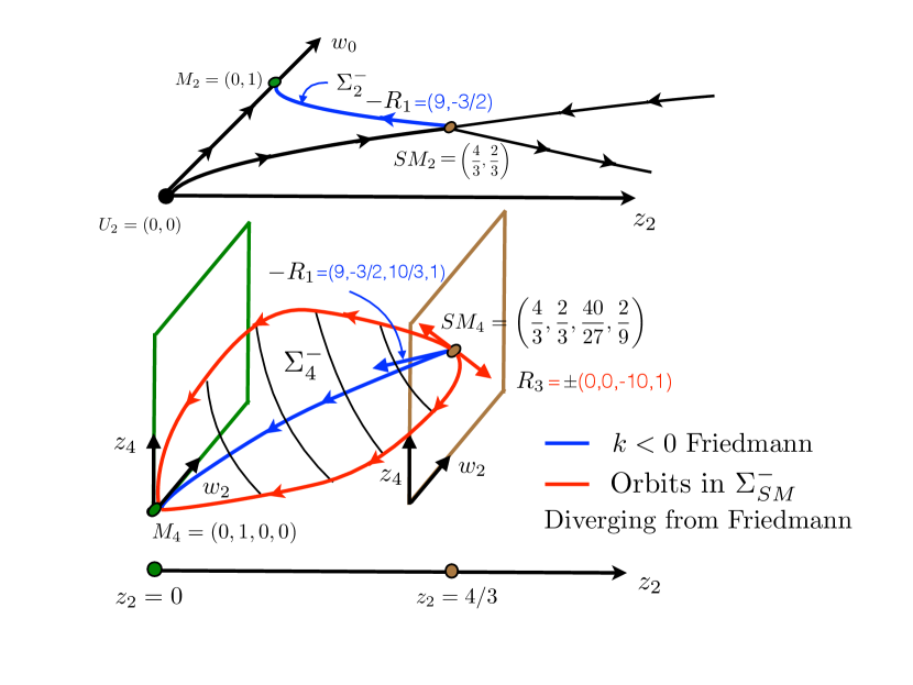
The time since the Big Bang gauge choice is assumed in Figure 3, so all elements of \mathcal{F} agree with k<0k<0 Friedmann at leading order, that is, they lie on the unstable trajectory taking SMSM to MM in the leading order phase portrait associated with (1.20)–(1.21). This is denoted by ΣSM\Sigma_{SM}^{-} in Figure 3, with Σ2\Sigma_{2}^{-} and Σ4\Sigma_{4}^{-} specifying the unstable manifold for the 2×22\times 2 and 4×44\times 4 systems respectively. The phase portraits of Figures 1 and 3 are consistent because the first two components of 𝑹1-\boldsymbol{R}_{1} give the direction of the trajectory which connects SM2SM_{2} to M2M_{2} at level n=1n=1 and the second two components represent the higher order corrections. The projections of the k<0k<0 Friedmann solutions onto solutions of the STV-ODE of orders n=1n=1 and n=2n=2 are represented by the blue curves in Figure 3. Note that the presence of a second positive eigenvalue λA2=43\lambda_{A2}=\frac{4}{3} implies the unstable manifold of SMSM intersects \mathcal{F} in a two dimensional space of trajectories emanating from SMSM. We prove that only the eigensolution of λA1\lambda_{A1} corresponds to the Friedmann spacetime at order n=2n=2. This immediately implies that there exist solutions in the unstable manifold of SMSM which agree with a k<0k<0 Friedmann spacetime at order n=1n=1 but diverge from Friedmann at intermediate times. Since all solutions in \mathcal{F} decay to MM as tt\to\infty, this implies that solutions in the unstable manifold of SMSM agree with k<0k<0 Friedmann in the limits t0t\to 0, tt\to\infty and at leading order n=1n=1, but which diverge, and hence introduce accelerations away from Friedmann, at intermediate times. By the Hartman–Grobman Theorem, nonlinear solutions correspond to linearized solutions in a neighborhood of a rest point, so solutions in the unstable manifold of SMSM are determined by their limiting eigendirection 𝑹=a𝑹1+b𝑹3\boldsymbol{R}=a\boldsymbol{R}_{1}+b\boldsymbol{R}_{3} at SMSM, and hence we conclude that the magnitude of the acceleration away from Friedmann is measured by ba\frac{b}{a}, which can be arbitrarily large. We state this precisely in the following theorem.

Theorem 5 (Partial statement of Theorem 40).

All solutions in the unstable manifold of SMSM at order n=2n=2 leave SMSM tangent to

𝑼(τ)=aeλA1(ττ0)𝑹A1+beλA2(ττ0)𝑹A2,\displaystyle\boldsymbol{U}(\tau)=ae^{\lambda_{A1}(\tau-\tau_{0})}\boldsymbol{R}_{A1}+be^{\lambda_{A2}(\tau-\tau_{0})}\boldsymbol{R}_{A2}, (1.24)

where

λA1\displaystyle\lambda_{A1} =23,\displaystyle=\frac{2}{3}, 𝑹A1\displaystyle\boldsymbol{R}_{A1} =(9321031);\displaystyle=\left(\begin{array}[]{c}9\\ -\frac{3}{2}\\ \frac{10}{3}\\ 1\end{array}\right); λA2\displaystyle\lambda_{A2} =43,\displaystyle=\frac{4}{3}, 𝑹A2\displaystyle\boldsymbol{R}_{A2} =(00101);\displaystyle=\left(\begin{array}[]{c}0\\ 0\\ -10\\ 1\end{array}\right); (1.33)

are the eigenpairs spanning the unstable manifold of the linearization of the 4×44\times 4 system of STV-ODE (1.20)–(1.23) about the rest point SMSM and aa and τ0\tau_{0} are fixed constants determined by the unique k0k\neq 0 Friedmann spacetime at n=1n=1. The constant bb is then a second free parameter which describes the instability of the k0k\neq 0 Friedmann spacetime at SMSM at order n=2n=2.

Note that the smallest positive eigenvalue to emerge at any order at SMSM is λB3=13\lambda_{B3}=\frac{1}{3} and since all trajectories in \mathcal{F} have a non-zero component of 𝑹A1\boldsymbol{R}_{A1} by definition, we can further conclude that all trajectories in the unstable manifold of SMSM are tangent to 𝑹A1\boldsymbol{R}_{A1} in backward time at SMSM in the phase portrait of the STV-ODE of order n=2n=2 but come in tangent to 𝑹B3\boldsymbol{R}_{B3} at SMSM in the portraits of the STV-ODE at all higher orders. We show in Theorem 48 that the k<0k<0 Friedmann solution has no components in direction 𝑹B3\boldsymbol{R}_{B3} and that by the nested structure of the STV-ODE, 𝑹Bn\boldsymbol{R}_{Bn} has non-zero components in only leading order entries.

The existence of a unique negative eigenvalue λB2=13\lambda_{B2}=-\frac{1}{3} at order n=2n=2 implies that SMSM is an unstable saddle rest point, but not an unstable source. From this we conclude that not all solutions in \mathcal{F} lie in the unstable manifold of SMSM, even though they decay time asymptotically to MM as tt\to\infty. Since SMSM is a saddle rest point, backward time trajectories in \mathcal{F} starting near SMSM will not typically tend to SMSM, but rather, indicative of the standard phase portrait of a saddle rest point, will generically follow the backward time trajectory of the stable manifold at SMSM. This implies the Big Bang is self-similar like the critical (k=0k=0) Friedmann spacetime only at leading order n=1n=1 but generically not self-similar at higher orders, as recorded in Theorem 4 above. We conclude that the time evolution of perturbations of SMSM becomes indistinguishable from k<0k<0 Friedmann solutions at late times after the Big Bang, agrees exactly with the same k<0k<0 Friedmann solution in the leading order phase portrait, including the limits t0t\to 0 and \infty, but introduce anomalous accelerations away from k<0k<0 Friedmann spacetimes at intermediate times, starting at order n=2n=2. This provides a rigorous mathematical framework and mechanism for determining and explaining the source of the corrections to redshift vs luminosity computed numerically in [29], that is, created by the instability of SMSM.

The new parameter β\beta associated with (λA2,𝑹A2)(\lambda_{A2},\boldsymbol{R}_{A2}) naturally introduces accelerations away from Friedmann spacetimes at order ξ2\xi^{2} in ww, and hence order ξ3\xi^{3} in the velocity vv. These mimic the effects of a cosmological constant at third order in redshift factor z\rm{z} vs luminosity distance dd_{\ell}, as measured from the center [29]. This is the order of the discrepancy between the prediction of Friedmann spacetimes with a cosmological constant and Friedmann spacetimes without one. According to Figure 3, at late times after the Big Bang we should expect to observe spacetimes close to k<0k<0 Friedmann, but not k=0k=0. Moreover, perturbations from k<0k<0 Friedmann spacetimes, including perturbations of SMSM on the k<0k<0 side of \mathcal{F} at early times after the Big Bang, diverge from k<0k<0 Friedmann spacetimes at intermediate times before they decay back to k<0k<0 Friedmann at late times. Regarding the intermediate times, the new free parameter β\beta associated with the unstable manifold of the critical k=0k=0 Friedmann spacetime (SMSM) is not present in pure k<0k<0 Friedmann spacetimes and this effect appears to mimic the effects of a cosmological constant at the order (third order in redshift factor looking out from the center) at which the predictions of a cosmological constant diverge from the predictions of the Friedmann spacetimes without one. Said differently, this theory identifies a one parameter family of corrections to Friedmann at order n=2n=2, with further corrections to Friedman determined by the positive eigenvalues of SMSM at higher orders, the higher the order the smaller the correction near the center.

More generally, it was proven in [29] that the order in redshift factor in the relation between redshift and luminosity looking out from the center of a spherically symmetric spacetime, is at the same order as ξ\xi in our theory here. The Hubble constant and the quadratic correction to redshift vs luminosity is determined at order n=1n=1 from v=w1ξv=w_{1}\xi and z2ξ2z_{2}\xi^{2} respectively, and hence w2ξ3w_{2}\xi^{3} determines the third order correction in red-shift factor with z4ξ4z_{4}\xi^{4} determining the fourth order term. Since one requires values of w2w_{2} and z4z_{4} to determine whether a solution trajectory lies in \mathcal{F}^{\prime}, it follows that the fourth order correction to red-shift vs luminosity would be required to determine whether or not a cosmology lies in the unstable manifold of SMSM, that is, to determine whether the Big Bang is self-similar like SMSM at all orders, or whether it diverges from self-similarity at order n=2n=2. We conclude that the family \mathcal{F} extends the k<0k<0 Friedmann spacetimes to a stable family of spacetimes, closed under small perturbation, which characterizes the instability of the critical (k=0k=0) and underdense (k<0k<0) Friedmann spacetimes to smooth radial perturbations.

1.7 The Canonical Spacetime at Order n=1n=1

When time since the Big Bang is imposed, every trajectory of the STV-ODE of order n=1n=1 reduces to SMSM or to a trajectory in its unstable manifold. In the underdense case, this is the unique trajectory which takes SM=(43,23)SM=(\frac{4}{3},\frac{2}{3}) to M=(0,1)M=(0,1) in the limit tt\to\infty at order n=1n=1. This trajectory, which we label (z2F(t),w0F(t))(z_{2}^{F}(t),w_{0}^{F}(t)), and its log-time translations provide a canonical leading order evolution shared by all underdense solutions in \mathcal{F}, including k<0k<0 Friedmann spacetimes. The resulting evolution κρ(t)=z2F(t)t2\kappa\rho(t)=z^{F}_{2}(t)t^{-2}, v(t)=w0F(t)rt1v(t)=w^{F}_{0}(t)rt^{-1} is therefore an explicit spacetime which is in a sense more fundamental than k<0k<0 Friedmann spacetimes because it is shared, under log-time translation, by all underdense solutions to leading order. In [29] we proved that Δ0\Delta_{0} and present time t0t_{0} in this leading order evolution are sufficient to uniquely determine the Hubble constant H0H_{0} and quadratic correction QQ in the relationship between redshift factor z\rm{z} vs luminosity distance dd_{\ell},

H01d=z+Qz2,\displaystyle H_{0}^{-1}d_{\ell}=\rm{z}+Q\rm{z}^{2},

as measured at the center of the spacetime, so long as 0.25Q0.50.25\leq Q\leq 0.5. Serendipitously, this latter constraint was shown in [29] to be consistent with k=0k=0 Friedmann augmented with 70% dark energy, the assumption of the ΛCDM\Lambda CDM model. Because of its fundamental nature, it is useful to have an explicit formula for (z2F(t),w0F(t))(z_{2}^{F}(t),w_{0}^{F}(t)), which is provided by Theorem 42 by extracting the leading order evolution from a known implicit formula for k<0k<0 Friedmann spacetimes [13]. The result is restated in the following theorem.

Theorem 6 (Partial statement of Theorem 42).

Define θ:(0,)(0,)\theta:(0,\infty)\to(0,\infty) by

θ(s)\displaystyle\theta(s) =f1(s),\displaystyle=f^{-1}(s),

where

s=f(θ)=12(sinh2θ2θ).\displaystyle s=f(\theta)=\frac{1}{2}(\sinh 2\theta-2\theta).

Then the functions

z2F(t)\displaystyle z_{2}^{F}(t) =z~2(θ(t))=6(sinh2θ(t)2θ(t))2(cosh2θ(t)1)3,\displaystyle=\tilde{z}_{2}(\theta(t))=\frac{6\big{(}\sinh 2\theta(t)-2\theta(t)\big{)}^{2}}{\big{(}\cosh 2\theta(t)-1\big{)}^{3}}, (1.34)
w0F(t)\displaystyle w_{0}^{F}(t) =w~0(θ(t))=(sinh2θ(t)2θ(t))sinh2θ(t)(cosh2θ(t)1)2,\displaystyle=\tilde{w}_{0}(\theta(t))=\frac{\big{(}\sinh 2\theta(t)-2\theta(t)\big{)}\sinh 2\theta(t)}{\big{(}\cosh 2\theta(t)-1\big{)}^{2}}, (1.35)

provide exact formulas for the particular solution of the 2×22\times 2 system (1.9)–(1.10) which traverses the trajectory connecting SMSM to MM in Figure 1, that is,

limt0(z2F(t),w0F(t))\displaystyle\lim_{t\to 0}\big{(}z_{2}^{F}(t),w_{0}^{F}(t)\big{)} =(43,23)=SM,\displaystyle=\bigg{(}\frac{4}{3},\frac{2}{3}\bigg{)}=SM, limt(z2F(t),w0F(t))\displaystyle\lim_{t\to\infty}\big{(}z_{2}^{F}(t),w_{0}^{F}(t)\big{)} =(0,1)=M.\displaystyle=(0,1)=M.

Moreover, (z2F(t),w0F(t))(z_{2}^{F}(t),w_{0}^{F}(t)) is the leading order term in expansion (1.6)–(1.7) of the k<0k<0 Friedmann solution assuming tt is time since the Big Bang and Δ0=49\Delta_{0}=\frac{4}{9}, where Δ0=κ3ρ0R03\Delta_{0}=\frac{\kappa}{3}\rho_{0}R_{0}^{3} parameterizes the k0k\neq 0 Friedmann solutions in their standard formulation. Furthermore, the corresponding formula for the leading order part of a Friedmann spacetime in terms of general Δ0>0\Delta_{0}>0 is then given by:

z2F(tΔ0)\displaystyle z_{2}^{F}\bigg{(}\frac{t}{\Delta_{0}}\bigg{)} =z~2(θ(tΔ0)),\displaystyle=\tilde{z}_{2}\bigg{(}\theta\bigg{(}\frac{t}{\Delta_{0}}\bigg{)}\bigg{)}, w0F(tΔ0)\displaystyle w_{0}^{F}\bigg{(}\frac{t}{\Delta_{0}}\bigg{)} =w~0(θ(tΔ0)).\displaystyle=\tilde{w}_{0}\bigg{(}\theta\bigg{(}\frac{t}{\Delta_{0}}\bigg{)}\bigg{)}. (1.36)

The approximate solution of the STV-PDE which corresponds to the n=1n=1 trajectory (z2F(t),w0F(t))(z_{2}^{F}(t),w_{0}^{F}(t)) is

𝑼F(t,ξ)=(zF(t,ξ),wF(t,ξ))(z2F(t)ξ2,w0F(t)).\displaystyle\boldsymbol{U}_{F}(t,\xi)=(z_{F}(t,\xi),w_{F}(t,\xi))\approx\big{(}z_{2}^{F}(t)\xi^{2},w_{0}^{F}(t)\big{)}.

Substituting z=κρr2z=\kappa\rho r^{2} and v=wξv=w\xi gives the equivalent SSC approximate solution

𝑾F(t,r)=(κρF(t,r),vF(t,r))(z2F(t)r2t2,w0F(t)rt1).\displaystyle\boldsymbol{W}_{F}(t,r)=(\kappa\rho_{F}(t,r),v_{F}(t,r))\approx\big{(}z_{2}^{F}(t)r^{2}t^{-2},w_{0}^{F}(t)rt^{-1}\big{)}.

The approximate solutions 𝑼F(t,ξ)\boldsymbol{U}_{F}(t,\xi) and 𝑾F(t,r)\boldsymbol{W}_{F}(t,r) describe the time asymptotics of solutions in \mathcal{F} as recorded in the following corollary.

Corollary 7.

Let 𝐔(t,ξ)=(z(t,ξ),w(t,ξ))\boldsymbol{U}(t,\xi)=(z(t,\xi),w(t,\xi)) be a solution in \mathcal{F} which determines 𝐖(t,r)=(κρ(t,r),v(t,r))\boldsymbol{W}(t,r)=(\kappa\rho(t,r),v(t,r)) through z=κρr2z=\kappa\rho r^{2} and v=wξv=w\xi. Then there exists a Δ0>0\Delta_{0}>0 such that

𝑾(t,r)WF(tΔ0,r)\displaystyle\boldsymbol{W}(t,r)\to W_{F}\bigg{(}\frac{t}{\Delta_{0}},r\bigg{)}

as tt\to\infty at each fixed r>0r>0, with errors O(t5r2)O(t^{-5}r^{-2}) and O(t3r3)O(t^{-3}r^{3}) in ρ\rho and vv respectively; and

𝑾(t,r)WF(tΔ0,r)\displaystyle\boldsymbol{W}(t,r)\to W_{F}\bigg{(}\frac{t}{\Delta_{0}},r\bigg{)}

as r0r\to 0 at each fixed t>0t>0, with errors O(t4r2)O(t^{-4}r^{2}) and O(t3r3)O(t^{-3}r^{3}) in ρ\rho and vv respectively. Moreover, 𝐔F(tΔ0,r)\boldsymbol{U}_{F}(\frac{t}{\Delta_{0}},r) agrees to the same orders with the unique k<0k<0 Friedmann spacetime determined by Δ0\Delta_{0}.

1.8 Conclusions

The Friedmann spacetimes in the limit p=0p=0, with or without a cosmological constant, have been the accepted large scale model for late stage Big Bang Cosmology since Hubble’s measurement of the expanding Universe in 1929. In the modern theory of Cosmology, the zero pressure Friedmann model applies after the time when the pressure drops precipitously to zero, some 10,000 years after the Big Bang, about an order of magnitude before the decoupling of radiation and matter gives rise to the microwave background radiation [17]. The widely accepted ΛCDM\Lambda CDM standard model for the large scale expansion of the Universe is a critically expanding k=0k=0 Friedmann spacetime with dark energy modeled by a positive cosmological constant, which is negligible relative to the energy density at early times. In this model, dark energy accounts for approximately 70% of the energy density of the Universe at present time [29]. We propose \mathcal{F} as an extension of the k0k\leq 0 Friedmann spacetimes to a stable family of cosmological models which reduce to k<0k<0 Friedmann in the time asymptotic limit tt\to\infty (for fixed rr) but naturally introduce anomalous accelerations relative to the Friedmann spacetimes at early and intermediate times into the dynamics of solutions of the Einstein field equations, without recourse to a cosmological constant. This confirms mathematically that a direct consequence of Einstein’s original theory of General Relativity, without a cosmological constant or dark energy, is that one can expect to observe a close approximation to non-critical (k0k\neq 0) Friedmann spacetimes at late times after the Big Bang, but not critical (k=0k=0) Friedmann spacetimes.111111The density is too large for a cosmological constant of the current observed magnitude to influence the stability of SMSM early on during the Big Bang at the onset of the instability when the pressure drops to zero [29].

The presence of solutions in the stable manifold \mathcal{F}^{\prime} of SMSM that are different from k<0k<0 Friedmann spacetimes tells us that general perturbations of k<0k<0 Friedmann spacetimes in \mathcal{F}^{\prime}, as well as underdense perturbations of the k=0k=0 Friedmann spacetime, at early times after the Big Bang produce accelerations away from Friedmann solutions before they decay back to k<0k<0 Friedmann as tt\to\infty (for fixed rr). Thus anomalous accelerations away from k0k\leq 0 Friedmann spacetimes are not a violation, but a prediction of Einstein’s original theory of General Relativity without a cosmological constant, and such does not change the picture during the early epoch when the cosmological constant is negligible relative to the energy density.121212As in [29], it is interesting to consider whether this might explain some of the conundrums with the Standard Model of Cosmology, such as the variable cosmological constant, the flatness problem or the uniform temperature problem. The present paper focuses only on the mathematics, the intention is to address the aforementioned problems in future publications.

The definitive description of the instability of the critical Friedmann spacetime in terms of the family of spacetimes \mathcal{F} set out here provides new insights for exploring the hypothesis that the observed anomalous acceleration of the galaxies might be explained within Einstein’s original theory of General Relativity without the cosmological constant, that is, the possibility that the Universe on the largest scale has evolved from a smooth perturbation of SMSM shortly after the Big Bang, such that the resulting solution lies within the family \mathcal{F}, with our galaxy near the center of that expansion. This possibility appears more intriguing for two reasons: First, the instability of SMSM to perturbations at every order makes the k=0k=0 Friedmann spacetime implausible as a physically observable model, with or without dark energy, and second, our theory here establishes that solutions in \mathcal{F}, the space of solutions into which underdense perturbations of SMSM will evolve, generically admit solutions which accelerate away from k<0k<0 Friedmann spacetimes as they evolve away from SMSM and before they decay back to k<0k<0 Friedmann solutions as tt\to\infty at all orders of the STV-ODE, qualitatively rich enough to mimic the effects of dark energy. Moreover, as demonstrated in [29], the acceleration at the order of the quadratic term in lies within the narrow range 0.25Q0.50.25\leq Q\leq 0.5, consistent with the effects of a cosmological constant Λ0.7\Lambda\approx 0.7.

We comment that in [31] the authors also proposed a wave model alternative to dark energy in which a self-similar solution of the p0p\neq 0 perfect fluid Einstein field equations, interpreted as a local time-asymptotic wave pattern at the end of the Radiation Dominated Epoch,131313When the pressure drops precipitously to p=0p=0 at about 10,000 years after the Big Bang, an order of magnitude before the uncoupling of matter and radiation around 300,000 years after the Big Bang. induces an underdensity which triggers an instability in SMSM when the pressure drops to zero. This was modeled as a mechanism for creating the observed anomalous acceleration of the galaxies observed at present time. For this, authors in [31] identified a one parameter family of self-similar solutions of the perfect fluid Einstein field equations, parameterized by the so-called acceleration parameter aa, such that a=1a=1 is the k=0k=0 Friedmann spacetime with equation of state p=c23ρp=\frac{c^{2}}{3}\rho.141414This is the equation of state for the state of matter known as pure radiation, as well as the equation of state for the extreme relativistic limit of free particles [34]. The authors proposed solutions in this family as candidates for time asymptotic wave patterns at the end of the Radiation Dominated Epoch of the Big Bang. These self-similar solutions produce perturbations of SMSM at the end of the Radiation Dominated Epoch and the authors introduced and employed a self-similar formulation of the SSC equations to numerically evolve the resulting perturbations up through the Matter Dominated Epoch to present time. As a result of this, a unique value of the acceleration parameter was identified which produced the correct Hubble constant H0H_{0} and quadratic correction QQ to redshift vs luminosity at present time. From this, a prediction was made at the third order C3C_{3} in the redshift factor in the expansion of redshift vs luminosity [31],

H01d=z+Qz2+C3z3+C4z4+,\displaystyle H_{0}^{-1}d_{\ell}=\rm{z}+Q\rm{z}^{2}+C_{3}\rm{z}^{3}+C_{4}\rm{z}^{4}+\dots,

where z\rm{z} is the redshift factor and dd_{\ell} is the luminosity. This was compared with the predictions of dark energy. The main principle is that an observer looking outward from the center at time t=t0t=t_{0} into a spacetime evolving as a solution in the family \mathcal{F} will measure the nthn^{th} order correction to redshift vs luminosity as a function of the coefficient of ξn\xi^{n} among v2n2(t0)ξ2n1=w2n2(t0)ξ2n2v_{2n-2}(t_{0})\xi^{2n-1}=w_{2n-2}(t_{0})\xi^{2n-2} and z2n(t0)ξ2nz_{2n}(t_{0})\xi^{2n}. Thus, in principle, there are the same number of parameters in an expansion of H01dH_{0}^{-1}d_{\ell} in powers of redshift z\rm{z} as there are initial conditions which can be freely assigned to determine a solution in \mathcal{F}. Thus the first through fourth order corrections are determined by z2z_{2}, w0w_{0}, z4z_{4} and w2w_{2} respectively, all determined by the STV-ODE of order n=2n=2.

Note that the unstable manifold \mathcal{F}^{\prime}\subset\mathcal{F} at order n=2n=2 of the STV-ODE is a two parameter surface in which the k<0k<0 Friedmann solutions account for only one of the two parameters, so k<0k<0 Friedmann spacetimes can only account for H0H_{0} and QQ, and then C3C_{3} is determined from these. The freedom to allow a two-parameter unstable manifold at order n=2n=2 allows one to freely assign C3C_{3}, but this then constrains the value of C4C_{4}. Finally, the freedom to assign z4z_{4} and w2w_{2} as two free parameters, in addition to z2z_{2} and w0w_{0}, is the right number of initial conditions to determine a general solution in \mathcal{F} at order n=2n=2. This then allows for the freedom to assign C4C_{4} as well. Although we confine ourselves here to the mathematics, our intention is to further explore the thesis proposed in [29], that is, that the instability of SMSM alone might account for experimental incongruencies, like a variable cosmological constant, associated with the observed anomalous acceleration of the galaxies, within Einstein’s original theory, without recourse to a cosmological constant.

As a final comment, we note that the STV-ODE describe the evolution of solutions along each line ξ=ξ0\xi=\xi_{0}, with ξ0\xi_{0} constant, and determine the time asymptotics of solutions implicitly from initial data starting from arbitrary initial time t0>0t_{0}>0, so any boundary condition at infinity is free to be imposed. Indeed, for solutions \mathcal{F}^{\prime} starting at time t=t0t=t_{0} on the underdense side of the stable manifold of SMSM in the n=1n=1 phase portrait in Figure 2, the limit at t=t=\infty is the rest point MM. The rest point MM emerges implicitly from the analysis in SSCNG coordinates and we surmise that this boundary condition would be difficult to guess ahead of time to impose as a boundary condition in different coordinate systems. For example, decay to rest point MM implies that the velocity vv aligns with ξ=rt\xi=\frac{r}{t} as the density tends to zero in smooth solutions of the Einstein field equations. It is interesting to note that when vξv\approx\xi, the SSCNG time coordinate diverges from comoving time except at r=0r=0, so the time asymptotics of the velocity would be difficult to guess from knowledge of solutions given in a comoving coordinate system alone. The effect of imposing any other boundary condition at infinity in a different coordinate system, like Lemaître–Tolman–Bondi coordinates, would necessarily break the smoothness condition at r=0r=0, leading to a singularity at the origin [22]. Moreover, the perturbations in \mathcal{F} do not represent simple under-densities relative to the critical k=0k=0 Friedmann solution because setting k=0k=0 as a boundary condition at infinity would not in general be consistent with solutions in \mathcal{F}. For one thing, solutions in the unstable manifold of SMSM which decay back to MM as tt\to\infty remain aligned with k<0k<0 Friedmann at leading order but incur an advancing or retarding of w2w_{2} which will be significant at intermediate times before the decay of the trajectory to MM takes over. In fact, this effect is exactly at the order of the measured anomalous acceleration [31]. The purpose of the present paper is to complete the mathematical theory of the pressureless self-similar Einstein field equations, give a definitive characterization of the instability of the critical Friedmann spacetime and to give a global description of underdense perturbations of SMSM in terms of the family \mathcal{F}. Authors will return to the problem of modeling redshifts in a subsequent publication.

1.9 Summary

In summary, the family \mathcal{F} characterizes the instability of the critical k=0k=0 Friedmann spacetime and the accelerations away from Friedmann are described quantitatively at every order by the STV-ODE. We identify a new positive and negative eigenvalue at SMSM in the phase portrait of the STV-ODE of order n=2n=2, different from the leading order eigenvalue associated with k<0k<0 Friedmann spacetimes. The positive eigenvalue produces a new free parameter which generates accelerations away from k<0k<0 Friedmann spacetimes within the unstable manifold \mathcal{F}^{\prime} of SMSM and the negative eigenvalue at SMSM produces accelerations away from k<0k<0 Friedmann spacetimes in \mathcal{F}, outside the unstable manifold \mathcal{F}^{\prime}. This directs us to an underlying mechanism which produces a consequential third order correction to redshift vs luminosity, the order of the discrepancy associated with dark energy, both within \mathcal{F}^{\prime} and its complement \mathcal{F}\setminus\mathcal{F}^{\prime}, different from the predictions made by k=0k=0 Friedmann spacetimes. In particular, this provides a deeper mathematical understanding of the source of the third order correction computed numerically in [29]. Such accelerations away from k0k\leq 0 Friedmann spacetimes are shown to be triggered by arbitrarily small perturbations of SMSM, a significant consequence of the instability of the k=0k=0 Friedmann spacetime to the subject of Cosmology. The authors intend to address the physical redshift vs luminosity problem quantitatively from this point of view in a forthcoming paper.

1.10 Outline of Paper

In Section 2 we summarize the main results in this paper. In Section 3 we explain the condition for a spherically symmetric solution of the Einstein field equations to be smooth at the center of symmetry. Our requirement for smoothness at the center is simply that the nonzero terms in the expansion of the solution in powers of ξ\xi should contain only even powers ξ2n\xi^{2n}. In particular, this implies that smooth solutions solve the STV-ODE at each order nn. In Section 4 we demonstrate that the time since the Big Bang gauge forces every trajectory at order n=1n=1 to agree with a k0k\neq 0 Friedmann spacetime. In Section 5 we review the Friedmann spacetimes in comoving coordinates and derive simple general formulas for coordinate transformations which take spherically symmetric metrics to SSCNG. In Section 6 we give a new simpler proof of the self-similarity of the k=0k=0 Friedmann spacetime in SSCNG coordinates for equations of state of the form p=σρp=\sigma\rho. In Section 7 we present a new derivation of the STV-PDE, which includes the case of non-zero pressure by incorporating the equation of state p=σρp=\sigma\rho into the equations. In Section 8 we derive the STV-ODE of order n=2n=2 by expanding the STV-PDE in even powers of ξ\xi. In Section 9 we discuss the STV-ODE at orders n=1n=1 and n=2n=2 and we incorporate the k0k\leq 0 Friedmann solutions into these systems. In Section 10 we characterize the unstable manifolds of SMSM at orders n=1n=1 and n=2n=2 and identify a new free parameter β\beta in the unstable manifold of SMSM at order n=2n=2, not accounted for by k<0k<0 Friedmann solutions. In Section 11 we discuss the higher order STV-ODE and prove that all solutions which tend to the rest point MM at order n=1n=1 also converge to MM at all higher orders n>1n>1. In Section 12 we prove that the k<0k<0 Friedmann spacetimes are pure eigensolutions of the STV-ODE up to order n=3n=3. The first appendix, Section 13 are where some of the more technical proofs are given. The second appendix, Section 14, is where we make the connections between the Theorems stated in [29], which used a different notation and were stated without proof, and the results in this paper. Finally, in the third appendix, Section 15, we discuss Lemaître–Tolman–Bondi coordinates.

2 Statement of Results

We start by recording the following result, which asserts that self-similar coordinates are valid out to approximately the Hubble radius.

Theorem 8 (Informal statement of Theorems 24 and 26).

The mapping (t,r)(t,ξ)(t,r)\to(t,\xi) is a regular one-to-one mapping of the SSC (t,r)(t,r) to self-similar coordinates (t,ξ)(t,\xi) for all |ξ|ξ00.816|\xi|\leq\xi_{0}\approx 0.816.

In the theorem below we derive our most general version of the STV-PDE, that is, for perfect fluid spacetimes with equation of state p=σρp=\sigma\rho with σ\sigma constant.

Theorem 9 (Partial statement of Theorem 32).

Assume the equation of state p=σρp=\sigma\rho with constant σ\sigma. Then for |ξ|<ξ0|\xi|<\xi_{0}, the perfect fluid Einstein field equations with an SSC metric are equivalent to the following four equations in unknowns A(t,ξ)A(t,\xi), D(t,ξ)D(t,\xi), z(t,ξ)z(t,\xi) and w(t,ξ)w(t,\xi):

ξAξ\displaystyle\xi A_{\xi} =z+(1A),\displaystyle=-z+(1-A), (2.1)
ξDξ\displaystyle\xi D_{\xi} =D2A(2(1A)(1σ2)1v21+σ2v2z),\displaystyle=\frac{D}{2A}\bigg{(}2(1-A)-(1-\sigma^{2})\frac{1-v^{2}}{1+\sigma^{2}v^{2}}z\bigg{)}, (2.2)
tzt+ξ((1+Dw)z)ξ\displaystyle tz_{t}+\xi\big{(}(-1+Dw)z\big{)}_{\xi} =Dwz,\displaystyle=-Dwz, (2.3)
twt+(1+Dw)ξwξ\displaystyle tw_{t}+(-1+Dw)\xi w_{\xi} w+Dw2(1+σ2)σ2ξz(D(1v2)v2(1+σ2v2)2z)ξ\displaystyle-w+Dw^{2}-\frac{(1+\sigma^{2})\sigma^{2}}{\xi z}\bigg{(}D\frac{(1-v^{2})v^{2}}{(1+\sigma^{2}v^{2})^{2}}z\bigg{)}_{\xi}
+σ2ξz(D1v21+σ2v2zξ2)ξ=RHS,\displaystyle+\frac{\sigma^{2}\xi}{z}\bigg{(}D\frac{1-v^{2}}{1+\sigma^{2}v^{2}}\frac{z}{\xi^{2}}\bigg{)}_{\xi}=\text{RHS}, (2.4)

where

RHS=1ξ21v21+σ2v2D2A((1σ2)(1A)+2σ21v21+σ2v2z)\displaystyle\text{RHS}=-\frac{1}{\xi^{2}}\frac{1-v^{2}}{1+\sigma^{2}v^{2}}\frac{D}{2A}\bigg{(}(1-\sigma^{2})(1-A)+2\sigma^{2}\frac{1-v^{2}}{1+\sigma^{2}v^{2}}z\bigg{)}

and

w=1+σ21+σ2v2vξ.\displaystyle w=\frac{1+\sigma^{2}}{1+\sigma^{2}v^{2}}\frac{v}{\xi}. (2.5)

Theorem 9 reduces to Theorem 1 of the Introduction when p=σ=0p=\sigma=0, applicable to late time Big Bang Cosmology [17], the setting of this paper.

The authors’ original motivation to formulate a self-similar version of the Einstein field equations was the discovery that, when p=σρp=\sigma\rho and the usual gauge of proper time at r=0r=0 with the Big Bang at t=0t=0 is employed, the k=0k=0 Friedmann spacetime in SSC has the property that all of the variables AA, DD, zz and ww are functions of ξ=rt\xi=\frac{r}{t} alone, and hence represent a time independent solution, or rest point, of the STV-PDE, suggesting to the authors that such a PDE would be useful in studying the stability properties of the Standard Model of Cosmology. To state this precisely, we begin with the exact expression for the p=σρp=\sigma\rho, k=0k=0 Friedmann spacetimes in comoving coordinates (t,r)(t,r), which is given by Theorem 2 on page 88 of [26].

Theorem 10 (Partial statement of Theorem 29).

In comoving coordinates (t,r)(t,r), the k=0k=0 Friedmann metric with equation of state p=σρp=\sigma\rho takes the form

ds2=dt2+R(t)2(dr2+r2dΩ2),\displaystyle ds^{2}=-dt^{2}+R(t)^{2}\big{(}dr^{2}+r^{2}d\Omega^{2}\big{)}, (2.6)

where:

R(t)\displaystyle R(t) =t23(1+σ),\displaystyle=t^{\frac{2}{3(1+\sigma)}}, (2.7)
H(t)\displaystyle H(t) =23(1+σ)t,\displaystyle=\frac{2}{3(1+\sigma)t}, (2.8)
ρ(t)\displaystyle\rho(t) =43κ(1+σ)2t2,\displaystyle=\frac{4}{3\kappa(1+\sigma)^{2}t^{2}}, (2.9)

and the four velocity u\vec{u} satisfies

u=(u0,u1,u2,u3)=(1,0,0,0).\displaystyle\vec{u}=(u^{0},u^{1},u^{2},u^{3})=(1,0,0,0). (2.10)

To describe the mapping (t,r)(t¯,r¯)(t,r)\to(\bar{t},\bar{r}), which we prove takes (2.6) to SSC self-similar form, we note first that the SSC radial coordinate must be r¯=Rr\bar{r}=Rr to match the spheres of symmetry, that is,

r¯=R(t)r=tα2r,\displaystyle\bar{r}=R(t)r=t^{\frac{\alpha}{2}}r, (2.11)

where

α=43(1+σ).\displaystyle\alpha=\frac{4}{3(1+\sigma)}.

Next, we introduce the auxiliary variable η=r¯t\eta=\frac{\bar{r}}{t}, so that r¯=ηt\bar{r}=\eta t, and define the SSC time variable t¯\bar{t} in terms of η\eta by

t¯=F(η)t,\displaystyle\bar{t}=F(\eta)t, (2.12)

where

(η)=(1+α(2α)4η2)12α.\displaystyle\mathcal{F}(\eta)=\bigg{(}1+\frac{\alpha(2-\alpha)}{4}\eta^{2}\bigg{)}^{\frac{1}{2-\alpha}}. (2.13)

Then (2.11)–(2.13) define a mapping (t,r)(t¯,r¯)(t,r)\to(\bar{t},\bar{r}) by

(t¯,r¯)=(F(η)t,ηt)=(F(rtα21)t,rtα2)=:Φ(t,r).\displaystyle(\bar{t},\bar{r})=(F(\eta)t,\eta t)=\big{(}F\big{(}rt^{\frac{\alpha}{2}-1}\big{)}t,rt^{\frac{\alpha}{2}}\big{)}=:\Phi(t,r). (2.14)

The following theorem establishes that the mapping Φ:(t,r)(t¯,r¯)\Phi:(t,r)\to(\bar{t},\bar{r}) converts the p=σρp=\sigma\rho, k=0k=0 Friedmann spacetime to self-similar SSC form.

Theorem 11 (Informal statement of Theorem 30).

Assume |ξ|<ξ00.816|\xi|<\xi_{0}\approx 0.816. Then Φ\Phi in (2.14) defines a regular coordinate mapping and takes the p=σρp=\sigma\rho, k=0k=0 Friedmann spacetime to SSCSSC metric form

ds2=Bσdt2+1Aσdr2+r2dΩ2,\displaystyle ds^{2}=-B_{\sigma}dt^{2}+\frac{1}{A_{\sigma}}dr^{2}+r^{2}d\Omega^{2}, (2.15)

such that the metric components AσA_{\sigma}, BσB_{\sigma}, the density variable κρσr2\kappa\rho_{\sigma}r^{2} and velocity

vσ=1AσBσu¯σ1u¯σ0\displaystyle v_{\sigma}=\frac{1}{\sqrt{A_{\sigma}B_{\sigma}}}\frac{\bar{u}^{1}_{\sigma}}{\bar{u}_{\sigma}^{0}} (2.16)

are functions of the single variable η\eta according to:

Aσ\displaystyle A_{\sigma} =1(αη2)2,\displaystyle=1-\left(\frac{\alpha\eta}{2}\right)^{2}, (2.17)
Bσ\displaystyle B_{\sigma} =(1+α(2α)4η2)22α2α1(αη2)2,\displaystyle=\frac{\left(1+\frac{\alpha(2-\alpha)}{4}\eta^{2}\right)^{\frac{2-2\alpha}{2-\alpha}}}{1-\left(\frac{\alpha\eta}{2}\right)^{2}}, (2.18)
κρσr2\displaystyle\kappa\rho_{\sigma}r^{2} =34α2η2,\displaystyle=\frac{3}{4}\alpha^{2}\eta^{2}, (2.19)
vσ\displaystyle v_{\sigma} =α2η.\displaystyle=\frac{\alpha}{2}\eta. (2.20)

Moreover, η\eta is given implicitly as a function of ξ\xi by the the relation

ξ=rt=η(η).\displaystyle\xi=\frac{r}{t}=\frac{\eta}{\mathcal{F}(\eta)}.

Restricting to the case p=0p=0 and imposing the NG time gauge, solutions of the STV-PDE smooth at the center of symmetry admit the following formal expansion in even powers of ξ\xi. We include here the metric coefficients AA and D=ABD=\sqrt{AB} as well as the fluid variables zz and ww:

A(t,ξ)1\displaystyle A(t,\xi)-1 =A2(t)ξ2+A4(t)ξ4++A2n(t)ξ2n+,\displaystyle=A_{2}(t)\xi^{2}+A_{4}(t)\xi^{4}+\dotsc+A_{2n}(t)\xi^{2n}+\dots, (2.21)
D(t,ξ)1\displaystyle D(t,\xi)-1 =D2(t)ξ2+D4(t)ξ4++D2n(t)ξ2n+,\displaystyle=D_{2}(t)\xi^{2}+D_{4}(t)\xi^{4}+\dotsc+D_{2n}(t)\xi^{2n}+\dots, (2.22)
z(t,ξ)\displaystyle z(t,\xi) =z2(t)ξ2+z4(t)ξ4++z2n(t)ξ2n+,\displaystyle=z_{2}(t)\xi^{2}+z_{4}(t)\xi^{4}+\dotsc+z_{2n}(t)\xi^{2n}+\dots, (2.23)
w(t,ξ)\displaystyle w(t,\xi) =w0(t)+w2(t)ξ2++w2n2(t)ξ2n2+,\displaystyle=w_{0}(t)+w_{2}(t)\xi^{2}+\dotsc+w_{2n-2}(t)\xi^{2n-2}+\dots, (2.24)

with:

A0\displaystyle A_{0} =1,\displaystyle=1, D0\displaystyle D_{0} =1.\displaystyle=1. (2.25)

The STV-ODE are derived by substituting (2.21)–(2.24) into the STV-PDE and collecting like powers of ξ\xi. The equations close at every order n1n\geq 1 and we name the resulting systems the STV-ODE of order nn. Carrying this procedure out to order n=3n=3 is the subject of the following theorem.151515The STV-ODE of order n=3n=3 appear adequate for modeling redshift vs luminosity relations in Cosmology [29].

Theorem 12 (Partial statement of Corollary 47).

The STV-ODE computed up to order n=3n=3 are equivalent to the following system, which closes at every order:

tz˙2\displaystyle t\dot{z}_{2} =2z23z2w0,\displaystyle=2z_{2}-3z_{2}w_{0}, (2.26)
tw˙0\displaystyle t\dot{w}_{0} =16z2+ww02,\displaystyle=-\frac{1}{6}z_{2}+w-w_{0}^{2}, (2.27)
tz˙4\displaystyle t\dot{z}_{4} =4z45(z4w0+z2w2+z2w0D2),\displaystyle=4z_{4}-5(z_{4}w_{0}+z_{2}w_{2}+z_{2}w_{0}D_{2}), (2.28)
tw˙2\displaystyle t\dot{w}_{2} =110z4+3w24w0w212w02A212A22+12A2D2w02D2,\displaystyle=-\frac{1}{10}z_{4}+3w_{2}-4w_{0}w_{2}-\frac{1}{2}w_{0}^{2}A_{2}-\frac{1}{2}A_{2}^{2}+\frac{1}{2}A_{2}D_{2}-w_{0}^{2}D_{2}, (2.29)
tz˙6\displaystyle t\dot{z}_{6} =6z67(z6w0+z2w4+z2w0D4+z2w2D2+z4w0D2+z4w2),\displaystyle=6z_{6}-7(z_{6}w_{0}+z_{2}w_{4}+z_{2}w_{0}D_{4}+z_{2}w_{2}D_{2}+z_{4}w_{0}D_{2}+z_{4}w_{2}), (2.30)
tw˙4\displaystyle t\dot{w}_{4} =114z6+5w46w0w412w02(A4A22)12w02A2D2\displaystyle=-\frac{1}{14}z_{6}+5w_{4}-6w_{0}w_{4}-\frac{1}{2}w_{0}^{2}(A_{4}-A_{2}^{2})-\frac{1}{2}w_{0}^{2}A_{2}D_{2}
w0w2A2+12A2D4+12(A4A22)D2A2A4+12A23\displaystyle-w_{0}w_{2}A_{2}+\frac{1}{2}A_{2}D_{4}+\frac{1}{2}(A_{4}-A_{2}^{2})D_{2}-A_{2}A_{4}+\frac{1}{2}A_{2}^{3}
w02D44w0w2D23w22.\displaystyle-w_{0}^{2}D_{4}-4w_{0}w_{2}D_{2}-3w_{2}^{2}. (2.31)

Moreover,

A2\displaystyle A_{2} =13z2,\displaystyle=-\frac{1}{3}z_{2}, A4\displaystyle A_{4} =15z4,\displaystyle=-\frac{1}{5}z_{4}, A6\displaystyle A_{6} =17z6,\displaystyle=-\frac{1}{7}z_{6}, (2.32)

and:

D2\displaystyle D_{2} =112z2,\displaystyle=-\frac{1}{12}z_{2}, (2.33)
D4\displaystyle D_{4} =340z4+18z2w02196z22,\displaystyle=-\frac{3}{40}z_{4}+\frac{1}{8}z_{2}w_{0}^{2}-\frac{1}{96}z_{2}^{2}, (2.34)
D6\displaystyle D_{6} =112(z4w02+2z2w0w2+524z22w0223120z2z47288z2357z6).\displaystyle=\frac{1}{12}\bigg{(}z_{4}w_{0}^{2}+2z_{2}w_{0}w_{2}+\frac{5}{24}z_{2}^{2}w_{0}^{2}-\frac{23}{120}z_{2}z_{4}-\frac{7}{288}z_{2}^{3}-\frac{5}{7}z_{6}\bigg{)}. (2.35)

Consistent with (1.8), the STV-ODE are nested the sense that the equations of order n1n-1 are a closed subsystem of the STV-ODE of order nn. The following describes this nested structure of the STV-ODE in general.

Theorem 13 (Partial statement of Theorem 44).

Assume a smooth solution (A(t,ξ),D(t,ξ),z(t,ξ),w(t,ξ))(A(t,\xi),D(t,\xi),z(t,\xi),w(t,\xi)) of (1.2)–(1.5) is expanded in even powers of ξ\xi as in (2.21)–(2.24). Then A2kA_{2k} can be re-expressed in terms of z2kz_{2k}, and D2kD_{2k} can be re-expressed in terms of z2kz_{2k} and w0,,w2k2w_{0},\dots,w_{2k-2}, to form, at each order nn\in\mathbb{N}, a 2n×2n2n\times 2n system of ODE

t𝑼˙=𝑭n(𝑼)\displaystyle t\dot{\boldsymbol{U}}=\boldsymbol{F}_{n}(\boldsymbol{U}) (2.36)

in unknowns

𝑼=(𝒗1,,𝒗n)T,\displaystyle\boldsymbol{U}=(\boldsymbol{v}_{1},\dots,\boldsymbol{v}_{n})^{T},

where

𝒗k=(z2k,w2k2)T.\displaystyle\boldsymbol{v}_{k}=(z_{2k},w_{2k-2})^{T}.

Moreover, system (2.36) takes the component form

ddτ(𝒗1𝒗2𝒗n)=(P1𝒗1+𝒒1P2𝒗2+𝒒2Pn𝒗n+𝒒n),\displaystyle\frac{d}{d\tau}\left(\begin{array}[]{c}\boldsymbol{v}_{1}\\ \boldsymbol{v}_{2}\\ \vdots\\ \boldsymbol{v}_{n}\end{array}\right)=\left(\begin{array}[]{c}P_{1}\boldsymbol{v}_{1}+\boldsymbol{q}_{1}\\ P_{2}\boldsymbol{v}_{2}+\boldsymbol{q}_{2}\\ \vdots\\ P_{n}\boldsymbol{v}_{n}+\boldsymbol{q}_{n}\end{array}\right), (2.45)

where

Pk=Pk(𝒗1)=((2k+1)(1w0)1(2k+1)z214k+2(2k+2)(1w0)1)\displaystyle P_{k}=P_{k}(\boldsymbol{v}_{1})=\left(\begin{array}[]{cc}(2k+1)(1-w_{0})-1&-(2k+1)z_{2}\\ -\frac{1}{4k+2}&(2k+2)(1-w_{0})-1\end{array}\right) (2.48)

depends only on 𝐯1=(z2,w0)T\boldsymbol{v}_{1}=(z_{2},w_{0})^{T} and 𝐪k\boldsymbol{q}_{k} depends only on lower order terms:

𝒒1\displaystyle\boldsymbol{q}_{1} =𝟎,\displaystyle=\boldsymbol{0},
𝒒k\displaystyle\boldsymbol{q}_{k} =𝒒k(𝒗1,,𝒗k1),\displaystyle=\boldsymbol{q}_{k}(\boldsymbol{v}_{1},\dots,\boldsymbol{v}_{k-1}),

for each k=2,,nk=2,\dots,n.

The STV-ODE of order nn all admit the rest points SMSM and MM. The coordinates of the rest point SMSM are obtained by expanding the self-similar formulation of the k=0k=0 Friedmann spacetime in even powers of ξ\xi about the center. Alternatively, since the k=0k=0 Friedmann spacetime is a time independent solution of the STV-PDE, it follows that the resulting expansion gives the coordinates of the rest point SMSM at every order. The rest point MM, which represents Minkowski spacetime in the limit ρ0\rho\to 0, vξv\to\xi, has zeros in all entries except for a 11 in the (second) w0w_{0}-entry, that is, M=(0,1,0,,0)M=(0,1,0,\dots,0). It is easy to verify MM is a rest point by induction using (2.45). We record the rest points SMSM and MM, together with their eigenpairs as follows.

Theorem 14.

Each STV-ODE of order n1n\geq 1 admit the rest points:

M\displaystyle M =(0,1,0,,0)2n,\displaystyle=(0,1,0,\dots,0)\in\mathbb{R}^{2n}, SM\displaystyle SM =(43,23,4027,29,).\displaystyle=\bigg{(}\frac{4}{3},\frac{2}{3},\frac{40}{27},\frac{2}{9},\dots\bigg{)}. (2.49)

The rest point MM is a degenerate stable rest point with one eigenvalue and one eigenvector given by:

λM\displaystyle\lambda_{M} =1,\displaystyle=-1, 𝑹M\displaystyle\boldsymbol{R}_{M} =(0,1,0,1,)T.\displaystyle=(0,1,0,1,\dots)^{T}. (2.50)

The eigenvalues of SMSM, computable directly from (2.48), are given by:

λAn\displaystyle\lambda_{An} =2n3,\displaystyle=\frac{2n}{3}, λBn\displaystyle\lambda_{Bn} =13(2n5).\displaystyle=\frac{1}{3}(2n-5). (2.51)

The corresponding eigenvectors up to order n=2n=2 are given by:

λA1\displaystyle\lambda_{A1} =23,\displaystyle=\frac{2}{3}, 𝑹1:=𝑹A1\displaystyle\boldsymbol{R}_{1}:=\boldsymbol{R}_{A1} =(9,32,103,1)T;\displaystyle=\bigg{(}-9,\frac{3}{2},-\frac{10}{3},-1\bigg{)}^{T}; (2.52)
λB1\displaystyle\lambda_{B1} =1,\displaystyle=-1, 𝑹B1\displaystyle\boldsymbol{R}_{B1} =(4,1,809,1)T;\displaystyle=\bigg{(}4,1,\frac{80}{9},1\bigg{)}^{T}; (2.53)
λA2\displaystyle\lambda_{A2} =43,\displaystyle=\frac{4}{3}, 𝑹3:=𝑹A2\displaystyle\boldsymbol{R}_{3}:=\boldsymbol{R}_{A2} =(0,0,10,1)T;\displaystyle=(0,0,-10,1)^{T}; (2.54)
λB2\displaystyle\lambda_{B2} =13,\displaystyle=-\frac{1}{3}, 𝑹B2\displaystyle\boldsymbol{R}_{B2} =(0,0,203,1)T.\displaystyle=\bigg{(}0,0,\frac{20}{3},1\bigg{)}^{T}. (2.55)

Theorem 14 follows from the calculations given in Section 9 below. A few comments are in order. To verify that MM is a rest point of the STV-ODE at every order n1n\geq 1 is a straightforward induction argument based on setting the right hand side of the STV-ODE (2.45) to zero and applying induction on nn. That it is a degenerate stable rest point with one eigenvalue and one eigenvector given by (2.50) can be verified again by induction based on computing d𝑭n(M)d\boldsymbol{F}_{n}(M) from (2.48) and using the nested property of equations (2.45). The components of the rest point SMSM can be computed two different ways: First, by setting the right hand side of the STV-ODE (2.45) to zero and computing the zeros of 𝑭n(𝑼)\boldsymbol{F}_{n}(\boldsymbol{U}) in (2.48), assuming 𝑭n1(SM)=0\boldsymbol{F}_{n-1}(SM)=0, and second, they can be computed by expanding the self-similar form of the k=0k=0 Friedmann spacetime (2.17)–(2.20) in even powers of ξ\xi, such as is done in Section 12.

The SSCNG gauge, imposed in (2.25), still leaves open one last freedom in the SSCNG coordinate ansatz, namely, the invariance associated with time translation ttt0=t~t\to t-t_{0}=\tilde{t}, a transformation which preserves proper time at r=0r=0. This represents a redundancy of physical solutions of the STV-PDE and STV-ODE. We fix this gauge freedom for each solution separately by defining time since the Big Bang, that is, so the leading order solution agrees with SMSM or one of the trajectories in its unstable manifold, and hence agrees with a unique Friedmann spacetime in the 2×22\times 2 STV-ODE of order n=1n=1. From this, the STVODESTV-ODE of higher order n2n\geq 2 then characterize accelerations away from Friedmann spacetimes. The change of gauge to time since the Big Bang is developed carefully in Section 4. The general result is stated in the following lemma.

Lemma 15.

Let 𝐔(t,ξ)=(A(t,ξ),D(t,ξ),z(t,ξ),w(t,ξ))\boldsymbol{U}(t,\xi)=(A(t,\xi),D(t,\xi),z(t,\xi),w(t,\xi)) denote an arbitrary outgoing smooth solution of the STV-PDE (1.2)–(1.5) in SSCNG coordinates and let 𝐔~(t~,ξ~)\tilde{\boldsymbol{U}}(\tilde{t},\tilde{\xi}) denote the transformed solution of (1.2)–(1.5) obtained by making the NG gauge transformation:

t\displaystyle t tt0=t~,\displaystyle\to t-t_{0}=\tilde{t}, ξ\displaystyle\xi =(t~t~+t0)ξ~,\displaystyle=\bigg{(}\frac{\tilde{t}}{\tilde{t}+t_{0}}\bigg{)}\tilde{\xi},

so that

𝑼~(t~,ξ~)=𝑼(t~+t0,(t~t~+t0)ξ~).\displaystyle\tilde{\boldsymbol{U}}(\tilde{t},\tilde{\xi})=\boldsymbol{U}\bigg{(}\tilde{t}+t_{0},\bigg{(}\frac{\tilde{t}}{\tilde{t}+t_{0}}\bigg{)}\tilde{\xi}\bigg{)}.

Then for any given 𝐔\boldsymbol{U}, there exists a unique time translation ttt=t~t\to t-t_{*}=\tilde{t} such that the leading order part of 𝐔~\tilde{\boldsymbol{U}} is a solution which lies on the trajectories corresponding to the unstable manifold of SMSM or else agrees with SMSM itself.

The proof of Lemma 15 follows from calculations given in Section 4. Lemma 15 implies that the transformation tttt\to t-t_{*} maps solutions to solutions, and hence maps trajectories in \mathcal{F} at order nn to trajectories in \mathcal{F} for every n1n\geq 1. Note that the scaling τ=lnt\tau=\ln t, which converts the STV-ODE to an autonomous system, only exists for t>0t>0, so in this sense the mapping tttt\to t-t_{*} does not in general map the entire solution on one trajectory to the entire solution on another, as represented in the phase portrait of the autonomous system described in Figure 1, but rather transformed trajectories end at the rest point UU. Nevertheless, after we accomplish the transformation to time since the Big Bang, we recover the whole Friedmann solution, so in the end this does not represent a real problem for this theory. Lemma 15 also tells us that imposing time since the Big Bang places the n=1n=1 trajectory of a solution in \mathcal{F} at SMSM, or on one of the two trajectories in the unstable manifold of SMSM at order n=1n=1. To study underdense perturbations of SMSM, we now always assume time since the Big Bang is imposed and restrict to the space of solutions \mathcal{F} of the STV-ODE whose leading order trajectory is the connecting orbit that takes SMSM to MM in the leading order phase portrait diagrammed in Figure 2. In other words, we restrict to 𝑼\boldsymbol{U}\in\mathcal{F} which satisfy

𝒗1(t)=(z2(t),w0(t))=(z2F(tΔ0),w0F(tΔ0))\displaystyle\boldsymbol{v}_{1}(t)=(z_{2}(t),w_{0}(t))=\bigg{(}z_{2}^{F}\bigg{(}\frac{t}{\Delta_{0}}\bigg{)},w_{0}^{F}\bigg{(}\frac{t}{\Delta_{0}}\bigg{)}\bigg{)}

for some Δ0\Delta_{0}, where Δ0\Delta_{0} determines the k<0k<0 Friedmann spacetime to which it agrees at leading order. The next theorem tells us that trajectories in \mathcal{F} tend to the rest point MM at all orders of the STV-ODE and provides a rate of decay.

Theorem 16 (Informal statement of Corollary 46).

Let 𝐔(t)=(𝐯1(t),,𝐯n(t))\boldsymbol{U}(t)=(\boldsymbol{v}_{1}(t),\dots,\boldsymbol{v}_{n}(t)) be a solution of the STV-ODE (2.45) of order nn such that

limt𝒗1(t)=(0,1)=M.\displaystyle\lim_{t\to\infty}\boldsymbol{v}_{1}(t)=(0,1)=M.

Then

limt𝑼(t)=M\displaystyle\lim_{t\to\infty}\boldsymbol{U}(t)=M

as a solution of the STV-ODE at every higher order n>1n>1. Moreover, there exists constants (C1,,Cn)(C_{1},\dots,C_{n}) such that:

𝒗1()(0,1)sup\displaystyle\|\boldsymbol{v}_{1}(\cdot)-(0,1)\|_{sup} C1lntt,\displaystyle\leq C_{1}\frac{\ln t}{t}, k\displaystyle k =1,\displaystyle=1, (2.56)
𝒗k()sup\displaystyle\|\boldsymbol{v}_{k}(\cdot)\|_{sup} Cklntt,\displaystyle\leq C_{k}\frac{\ln t}{t}, k\displaystyle k =2,,n,\displaystyle=2,\dots,n, (2.57)

where for each k{1,,n}k\in\{1,\dots,n\}, CkC_{k} depends only on initial data assigned at t0>0t_{0}>0,

𝒗1(t0)\displaystyle\boldsymbol{v}_{1}(t_{0}) =𝒗10,\displaystyle=\boldsymbol{v}_{1}^{0},
\displaystyle\vdots
𝒗k(t0)\displaystyle\boldsymbol{v}_{k}(t_{0}) =𝒗k0,\displaystyle=\boldsymbol{v}_{k}^{0},

that is, CkC_{k} depends only on the initial data up to order kk.

In other words, Theorem 16 tells us that if a trajectory tends to MM at leading order, then it tends to MM at all orders. Note that if the CnC_{n} in (2.56)–(2.57) are bounded by a uniform constant CC for every n1n\geq 1, then we can sum the geometric series and obtain an error in the approximation over all orders nn (assuming |ξ|<1|\xi|<1):

z(t,ξ)=k=1z2kξ2k=k=1nz2kξ2k+Error,\displaystyle z(t,\xi)=\sum_{k=1}^{\infty}z_{2k}\xi^{2k}=\sum_{k=1}^{n}z_{2k}\xi^{2k}+Error, (2.58)

where

|Error|=|k=n+1z2kξ2k|Clnttξ2k+21ξ2.\displaystyle|Error|=\bigg{|}\sum_{k=n+1}^{\infty}z_{2k}\xi^{2k}\bigg{|}\leq C\frac{\ln t}{t}\frac{\xi^{2k+2}}{1-\xi^{2}}. (2.59)

Summing the geometric series in (2.59) then gives us a formula for the rate at which an underlying solution of the STV-PDE decays to MM.

It follows from Lemma 15 that to characterize underdense perturbations of the k=0k=0 Friedmann spacetime, we can assume the time since the Big Bang gauge and define the family \mathcal{F} as the set of all solutions of the STV-PDE which lie on the trajectory that takes SMSM to MM in the leading order STV-ODE of order n=1n=1. In this gauge, tt measures time since the Big Bang in the sense that limt0+R(t)=\lim_{t\to 0^{+}}R(t)=\infty, where R(t)R(t) is the scale factor associated with the Friedmann spacetime it agrees with at leading order [1].

Recall that n\mathcal{F}_{n}, also referred to as \mathcal{F} at order nn, is the set of solutions of the STV-ODE of order nn which satisfy the property

𝒗1(t)=(z2F(tΔ0),w0F(tΔ0))\displaystyle\boldsymbol{v}_{1}(t)=\bigg{(}z_{2}^{F}\bigg{(}\frac{t}{\Delta_{0}}\bigg{)},w_{0}^{F}\bigg{(}\frac{t}{\Delta_{0}}\bigg{)}\bigg{)}

for some Δ0>0\Delta_{0}>0, that is, solutions which take SMSM to MM at order n=1n=1. Recall also that the family nn\mathcal{F}_{n}^{\prime}\subset\mathcal{F}_{n}, referred to as the set of trajectories in \mathcal{F}^{\prime} at order nn, is the subset of n\mathcal{F}_{n} in the unstable manifold of SMSM at order nn. The following theorem describes how solutions in n\mathcal{F}_{n} generically accelerate away from Friedmann spacetimes at every order n1n\geq 1 by characterizing the global dynamics of solutions in terms of the eigenvalues of SMSM and its unstable manifold n\mathcal{F}_{n}^{\prime}. Since all smooth radial underdense perturbations of SMSM evolve within the space of trajectories n\mathcal{F}_{n}, we interpret this as a quantitative characterization of the instability of the p=0p=0, k=0k=0 Friedmann spacetime to smooth radial underdense perturbations.

Theorem 17.

Let 𝐔(t)=(𝐯1(t),,𝐯n(t))\boldsymbol{U}(t)=(\boldsymbol{v}_{1}(t),\dots,\boldsymbol{v}_{n}(t)) denote a solution of the STV-ODE (2.36) of order nn in the family n\mathcal{F}_{n} so that

𝒗1(t)=(z2F(tΔ0),w0F(tΔ0))\displaystyle\boldsymbol{v}_{1}(t)=\bigg{(}z_{2}^{F}\bigg{(}\frac{t}{\Delta_{0}}\bigg{)},w_{0}^{F}\bigg{(}\frac{t}{\Delta_{0}}\bigg{)}\bigg{)}

for some Δ0>0\Delta_{0}>0. Then:

  1. (i)

    Trajectories in the unstable manifold 2\mathcal{F}_{2}^{\prime} of SMSM generically diverge from Friedmann spacetimes in the phase portrait of the STV-ODE of order n=2n=2, and hence, by the nested property of the STV-ODE, they generically diverge from Friedmann at all orders n>2n>2 as well.

  2. (ii)

    The character of the unstable manifold n\mathcal{F}_{n}^{\prime} of SMSM is determined at order n=2n=2 in the sense that a solution 𝑼(t)\boldsymbol{U}(t) is in the unstable manifold n\mathcal{F}_{n}^{\prime} at all orders n2n\geq 2 if and only if it is in 2\mathcal{F}_{2}^{\prime}, that is, if and only if (𝒗1(t),𝒗2(t))(\boldsymbol{v}_{1}(t),\boldsymbol{v}_{2}(t)) is in the unstable manifold 2\mathcal{F}_{2}^{\prime} of SMSM at order n=2n=2. This implies the unstable manifold n\mathcal{F}_{n}^{\prime} is a codimension one set of trajectories in n\mathcal{F}_{n} at every order n2n\geq 2 of the STV-ODE.

  3. (iii)

    By definition, solutions in \mathcal{F} all satisfy limt𝒗1(t)=SM\lim_{t\to\infty}\boldsymbol{v}_{1}(t)=SM but generically limt𝒗2(t)SM\lim_{t\to\infty}\boldsymbol{v}_{2}(t)\neq SM.

  4. (iv)

    The smallest positive eigenvalue at SMSM emerges at order n=3n=3 in λA3\lambda_{A3} (followed by λA1\lambda_{A1} at n=1n=1). This implies that solution trajectories in n\mathcal{F}_{n}^{\prime} enter tangent to the Friedmann trajectory at order n=1n=1 (and thus also n=2n=2) but enter tangent to the eigenvector of λB3\lambda_{B3} at all higher orders n3n\geq 3.

For point (i), this follows directly from the presence of two distinct positive eigenvalues λA1\lambda_{A1} and λA2\lambda_{A2} at SMSM in the STV-ODE of order n=2n=2. These determine two independent eigendirections in the unstable manifold 2\mathcal{F}_{2}^{\prime} of SMSM at order n=2n=2, with only the eigendirection of λA1\lambda_{A1} corresponding to k<0k<0 Friedmann spacetimes.

For point (ii), this follows directly from the fact that there exists only a single negative eigenvalue λB2\lambda_{B2} at SMSM at order n=2n=2 and all higher order eigenvalues λAn\lambda_{An} and λBn\lambda_{Bn} for n3n\geq 3 are positive.

For point (iii), this follows directly from the presence of the single negative eigenvalue λB2\lambda_{B2} above level n=1n=1. We interpret this as establishing that, unlike Friedmann spacetimes, solutions in \mathcal{F} exhibit a self-similar Big Bang only at leading order n=1n=1 but generically do not at higher orders.

3 Smoothness at the Center of Spherically Symmetric Spacetimes in SSCNG Coordinates

Our goal is to characterize the instability of the p=0p=0, k=0k=0 Friedmann spacetime to perturbations within the class of smooth solutions. Since r=0r=0 is a singular value in radial coordinates, we need a condition characterizing smoothness at the center (r=0r=0) in SSC (1.1). The results of this paper rely on the validity of approximating solutions by finite Taylor expansions about the center of symmetry, so the main issue is to guarantee that solutions are indeed smooth in a neighborhood of the center.

The Universe is not smooth on small scales, so our assumption is that the center is not special regarding the regularity assumed in the large scale approximation of the Universe. Smoothness, by which we mean derivatives of all orders can be taken, at a point PP in a spacetime manifold is determined by the atlas of coordinate charts defined in a neighborhood of PP. The regularity of tensors is identified with the regularity of tensor components expressed in the coordinate systems of the given atlas. Now spherically symmetric solutions given, in say, Lemaître–Tolman–Bondi (LTB) or SSC employ spherical coordinates (r,ϕ,θ)(r,\phi,\theta) for the spacelike surfaces at constant time. The subtly here is that r=0r=0 is a coordinate singularity in spherical coordinates and functions are defined only for the radial coordinate r0r\geq 0, however, a coordinate system must be specified in a neighborhood of r=0r=0 to impose the conditions for smoothness at the center. Of course, once we have the metric represented as smooth in coordinate system x\vec{x} on an initial data surface in a neighborhood of r=0r=0, the local existence theorem giving the smooth evolution of solutions from smooth initial data for the Einstein field equations would not alone suffice to obtain our smoothness condition, as one would still have to prove that this evolution preserved the metric ansatz.

Following [29], we begin by showing that this issue can be resolved relatively easily in SSC because the SSC are precisely the spherical coordinates associated with Euclidean coordinate charts defined in a neighborhood of r=0r=0. Based on this, we show below that the condition for smoothness of metric components and functions in SSC is simply that all odd order derivatives should vanish at r=0r=0.

Consider in more detail the problem of representing a smooth, spherically symmetric perturbation of a k0k\leq 0 Friedman spacetime. To start, assume the existence of a solution of Einstein’s field equations representing a large, smooth underdense region of spacetime that expands from the end of the Radiation Dominated Epoch out to present time. For smooth perturbations, there should exist a coordinate system in a neighborhood of the center of symmetry, in which the solution is represented as smooth. Assume we have such a coordinate system (t,𝒙)×3(t,\boldsymbol{x})\in\mathbb{R}\times\mathbb{R}^{3}, with 𝒙=0\boldsymbol{x}=0 at the center, and use the notation

x=(x0,x1,x2,x3)=(t,x,y,z)=(t,𝒙).\displaystyle\vec{x}=(x^{0},x^{1},x^{2},x^{3})=(t,x,y,z)=(t,\boldsymbol{x}).

Spherical symmetry makes it convenient to represent the spatial Euclidean coordinates 𝒙3\boldsymbol{x}\in\mathbb{R}^{3} in spherical coordinates (r,θ,ϕ)(r,\theta,\phi), with r=|𝒙|r=|\boldsymbol{x}|. Since generically, any spherically symmetric metric can be transformed locally to SSC form [31], we assume the spacetime represented in the coordinate system (t,r,θ,ϕ)(t,r,\theta,\phi) takes the SSC form (1.1). This is equivalent to the metric in Euclidean coordinates 𝒙\boldsymbol{x} taking the form

ds2=B(|𝒙|,t)dt2+dr2A(|𝒙|,t)+|𝒙|2dΩ2,\displaystyle ds^{2}=-B(|\boldsymbol{x}|,t)dt^{2}+\frac{dr^{2}}{A(|\boldsymbol{x}|,t)}+|\boldsymbol{x}|^{2}d\Omega^{2},

where:

r2\displaystyle r^{2} =x2+y2+z2,\displaystyle=x^{2}+y^{2}+z^{2},
rdr\displaystyle rdr =xdx+ydy+zdz,\displaystyle=xdx+ydy+zdz,
r2dr2\displaystyle r^{2}dr^{2} =x2dx2+y2dy2+z2dz2+2xydxdy+2xzdxdz+2yzdydz,\displaystyle=x^{2}dx^{2}+y^{2}dy^{2}+z^{2}dz^{2}+2xydxdy+2xzdxdz+2yzdydz, (3.1)

and

dx2+dy2+dz2=dr2+r2dΩ2.\displaystyle dx^{2}+dy^{2}+dz^{2}=dr^{2}+r^{2}d\Omega^{2}. (3.2)

To guarantee the smoothness of our perturbation of Friedman at the center, we assume a gauge in which:

B(t,r)\displaystyle B(t,r) =1+O(r2),\displaystyle=1+O(r^{2}), A(t,r)\displaystyle A(t,r) =1+O(r2),\displaystyle=1+O(r^{2}),

so that also

1A(t,r)=1+O(r2)=:1+A^(t,r)r2,\displaystyle\frac{1}{A(t,r)}=1+O(r^{2})=:1+\hat{A}(t,r)r^{2},

where the smoothness of AA is equivalent to the smoothness of A^\hat{A} for r>0r>0. This sets the SSC time gauge to proper time at r=0r=0 and makes the SSC locally inertial at r=0r=0 and t>0t>0, a first step in guaranteeing that our spherical perturbations of Friedman are smooth at the center. Keep in mind that without this gauge the SSC form is invariant under arbitrary transformation of time, so we are free to choose proper time at r=0r=0. The locally inertial condition at r=0r=0 simply imposes that the corrections to Minkowski at r=0r=0 are second order in rr, in particular, the SSC metric (5.29) tends to Minkowski as r0r\to 0. These assumptions make physical sense and their consistency is guaranteed by reversing the steps in the argument to follow. We now ask what conditions on the metric functions AA and BB are imposed by assuming the SSC metric be smooth when expressed in our original Euclidean coordinate chart (t,𝒙)(t,\boldsymbol{x}) defined in a neighborhood of a point at r=0r=0, t>0t>0.

To transform the SSC metric (5.29) to (t,𝒙)(t,\boldsymbol{x}) coordinates, use (3.2) to eliminate the r2dΩ2r^{2}d\Omega^{2} term and (3.1) to eliminate the dr2dr^{2} term to obtain

ds2\displaystyle ds^{2} =B(|𝒙|,t)dt2+dx2+dy2+dz2\displaystyle=-B(|\boldsymbol{x}|,t)dt^{2}+dx^{2}+dy^{2}+dz^{2} (3.3)
+A^(|𝒙|,t)(x2dx2+y2dy2+z2dz2+2xydxdy+2xzdxdz+2yzdydz).\displaystyle+\hat{A}(|\boldsymbol{x}|,t)\big{(}x^{2}dx^{2}+y^{2}dy^{2}+z^{2}dz^{2}+2xydxdy+2xzdxdz+2yzdydz\big{)}.

The smoothness of A^\hat{A} is equivalent to the smoothness of AA, and the smoothness of AA and BB for r>0r>0 guarantees the smoothness of the Euclidean spacetime metric (3.3) in (t,𝒙)(t,\boldsymbol{x}) coordinates everywhere except at 𝒙=0\boldsymbol{x}=0. For smoothness at 𝒙=0\boldsymbol{x}=0, we impose the condition that the metric components in (3.3) should be smooth functions of (t,𝒙)(t,\boldsymbol{x}) at 𝒙=0\boldsymbol{x}=0 as well. Note again that imposing smoothness in (t,𝒙)(t,\boldsymbol{x}) coordinates at 𝒙=0\boldsymbol{x}=0 is correct in the sense that it is preserved by the Einstein evolution equations. We now show that smoothness at 𝒙=0\boldsymbol{x}=0 in this sense is equivalent to requiring that the metric functions AA and BB satisfy the condition that all odd rr-derivatives vanish at r=0r=0. To see this, observe that a function f(r)f(r) represents a smooth spherically symmetric function of the Euclidean coordinates 𝒙\boldsymbol{x} at r=|𝒙|=0r=|\boldsymbol{x}|=0 if and only if the function

g(x)=f(|𝒙|)\displaystyle g(x)=f(|\boldsymbol{x}|)

is smooth at 𝒙=0\boldsymbol{x}=0. Assuming ff is smooth for r0r\geq 0 (by which we mean ff is smooth for r>0r>0, and one sided derivatives exist at r=0r=0) and taking the nthn^{th} derivative of gg from the left and right and setting them equal gives the smoothness condition

fn(0)=(1)nfn(0).\displaystyle f^{n}(0)=(-1)^{n}f^{n}(0).

We state this formally in the following lemma (see [29]).

Lemma 18.

A function f(r)f(r) of the radial coordinate r=|𝐱|r=|\boldsymbol{x}| represents a smooth function of the Euclidean coordinates 𝐱\boldsymbol{x} if and only if ff is smooth for r0r\geq 0 and all odd derivatives vanish at r=0r=0. Moreover, if any odd derivative f(n+1)(0)0f^{(n+1)}(0)\neq 0, then f(|𝐱|)f(|\boldsymbol{x}|) has a jump discontinuity in its n+1n+1 derivative, and hence a kink singularity in its nthn^{th} derivative at r=0r=0.

As an immediate consequence, we obtain the condition for smoothness of SSC metrics at r=0r=0, given in the following corollary.

Corollary 19.

The SSC metric (5.29) is smooth at r=0r=0 in the sense that the metric components in (3.3) are smooth functions of the Euclidean coordinates (t,𝐱)(t,\boldsymbol{x}) if and only if the component functions A(t,r)A(t,r), B(t,r)B(t,r) are smooth in time and smooth for r>0r>0, all odd one-sided rr-derivatives vanish at r=0r=0 and all even rr-derivatives are bounded at r=0r=0.

To conclude, solutions of the Einstein field equations in SSC have four unknowns: The metric components AA and BB, the density ρ\rho and the scalar velocity vv. It is easy to show that if the SSC metric components satisfy the condition that all odd order rr-derivatives vanish at r=0r=0, then the components of the unit four-velocity vector uμu^{\mu} associated with smooth curves that pass through r=0r=0 will have the same property.161616This implies that the coordinates are smooth functions of arc-length along curves passing through r=0r=0. Moreover, the scalar velocity vv will have the property that all even derivatives vanish at r=0r=0 because vv is an outward velocity which picks up a change of sign when represented in x\vec{x} coordinates. Thus smoothness of SSC solutions at r=0r=0 at fixed time is equivalent to requiring that the metric components satisfy the condition that all odd rr-derivatives vanish at r=0r=0. These then give conditions on SSC solutions equivalent to the condition that the solutions are smooth in the ambient Euclidean coordinate system x\vec{x}. Theorem 34 of Section 7 proves that smoothness in the coordinate system x\vec{x} at r=0r=0 at each t>0t>0 in this sense is preserved by the Einstein evolution equations for SSC metrics when p=0p=0. In particular, this demonstrates that our condition for smoothness of SSC metrics at r=0r=0 is equivalent to the well-posedness of solutions in the ambient Euclidean coordinates defined in a neighborhood of r=0r=0. Thus we obtain the condition for smoothness of SSC metrics at r=0r=0 based on the Euclidean coordinate systems associated with SSC and show this is preserved by the evolution of the Einstein field equations. Since smoothness of the SSC metric components in this sense is equivalent to smoothness of the x\vec{x}-coordinates with respect to arc-length along curves passing through r=0r=0, in this sense, our condition for smoothness is geometric.

4 Time Since the Big Bang

The SSC-PDE self-similar form of the Einstein field equations for spherically symmetric dust (p=0p=0) spacetimes has the advantage that the time translation freedom of the SSC metric ansatz enables one to scale the time so that the Big Bang singularity for a general smooth solution agrees with a Friedmann spacetime at leading order for some value of kk. We establish this directly now with an argument based on the STV-ODE of order n=1n=1, namely:

tz˙2\displaystyle t\dot{z}_{2} =2z23z2w0,\displaystyle=2z_{2}-3z_{2}w_{0}, (4.1)
tw˙0\displaystyle t\dot{w}_{0} =16z2+w0w02,\displaystyle=-\frac{1}{6}z_{2}+w_{0}-w_{0}^{2}, (4.2)

where:

w\displaystyle w =vξ,\displaystyle=\frac{v}{\xi}, z\displaystyle z =ρr21v2.\displaystyle=\frac{\rho r^{2}}{1-v^{2}}.

Solutions (z2(t),w0(t))(z_{2}(t),w_{0}(t)) of (4.1)–(4.2) give the leading order approximation:

w(t,ξ)\displaystyle w(t,\xi) =w0(t)+O(ξ2),\displaystyle=w_{0}(t)+O(\xi^{2}),
z(t,ξ)\displaystyle z(t,\xi) =z2(t)ξ2+O(ξ4).\displaystyle=z_{2}(t)\xi^{2}+O(\xi^{4}).

Consider now the effect of a time translation t^=tt0\hat{t}=t-t_{0} and set

ξ^=rt^,\displaystyle\hat{\xi}=\frac{r}{\hat{t}},

so that:

w^\displaystyle\hat{w} =vξ^=(tt0t)vξ=(tt0t)w,\displaystyle=\frac{v}{\hat{\xi}}=\left(\frac{t-t_{0}}{t}\right)\frac{v}{\xi}=\left(\frac{t-t_{0}}{t}\right)w,
z^\displaystyle\hat{z} =z^2(t^)ξ^2+O(ξ^4)=(ttt0)2z^2(t^)ξ2+O(ξ4).\displaystyle=\hat{z}_{2}(\hat{t})\hat{\xi}^{2}+O(\hat{\xi}^{4})=\left(\frac{t}{t-t_{0}}\right)^{2}\hat{z}_{2}(\hat{t})\xi^{2}+O(\xi^{4}).

Thus it makes sense at leading order to define:

w^0\displaystyle\hat{w}_{0} :=(tt0t)w0,\displaystyle:=\left(\frac{t-t_{0}}{t}\right)w_{0}, z^2\displaystyle\hat{z}_{2} :=(tt0t)2z2.\displaystyle:=\left(\frac{t-t_{0}}{t}\right)^{2}z_{2}.

Given that the SSC metric form is invariant under time translation and the SSC-PDE and SSC-ODE faithfully represent the SSC solutions in (t,ξ)(t,\xi) coordinates, we should expect that (z2(t),w0(t))(z_{2}(t),w_{0}(t)) should solve the leading order equations (4.1)–(4.2) if and only if (z^2(t^),w^0(t^))(\hat{z}_{2}(\hat{t}),\hat{w}_{0}(\hat{t})) do. It suffices to verify that if (z2(t),w0(t))(z_{2}(t),w_{0}(t)) solve (4.1)–(4.2), then (z^2(t^),w^0(t^))(\hat{z}_{2}(\hat{t}),\hat{w}_{0}(\hat{t})) do. To this end, assuming a solution (z2(t),w0(t))(z_{2}(t),w_{0}(t)) and substituting (z^2(t^),w^0(t^))(\hat{z}_{2}(\hat{t}),\hat{w}_{0}(\hat{t})) into (4.1)–(4.2), we obtain

t^z^˙2\displaystyle\hat{t}\dot{\hat{z}}_{2} =(tt)[(ttt)2z˙2+2(tt2)(ttt)z2]\displaystyle=(t-t_{*})\left[\left(\frac{t-t_{*}}{t}\right)^{2}\dot{z}_{2}+2\left(\frac{t_{*}}{t^{2}}\right)\left(\frac{t-t_{*}}{t}\right)z_{2}\right]
=(tt)[3t(ttt)2z2(w023)+2(tt2)(ttt)z2]\displaystyle=(t-t_{*})\left[-\frac{3}{t}\left(\frac{t-t_{*}}{t}\right)^{2}z_{2}\left(w_{0}-\frac{2}{3}\right)+2\left(\frac{t_{*}}{t^{2}}\right)\left(\frac{t-t_{*}}{t}\right)z_{2}\right]
=3z^2[ttt(w023)23(tt)]\displaystyle=-3\hat{z}_{2}\left[\frac{t-t_{*}}{t}\left(w_{0}-\frac{2}{3}\right)-\frac{2}{3}\left(\frac{t_{*}}{t}\right)\right]
=2z^23z^2w^0\displaystyle=2\hat{z}_{2}-3\hat{z}_{2}\hat{w}_{0}

and

t^w^˙0\displaystyle\hat{t}\dot{\hat{w}}_{0} =(tt)[(ttt)w˙0+tt2w0]\displaystyle=(t-t_{*})\left[\left(\frac{t-t_{*}}{t}\right)\dot{w}_{0}+\frac{t_{*}}{t^{2}}w_{0}\right]
=(tt)[1t(ttt)(16z2+w0w02)+tt2w0]\displaystyle=(t-t_{*})\left[\frac{1}{t}\left(\frac{t-t_{*}}{t}\right)\left(-\frac{1}{6}z_{2}+w_{0}-w_{0}^{2}\right)+\frac{t_{*}}{t^{2}}w_{0}\right]
=16z^2w^02+(ttt)w^0+ttw^0\displaystyle=-\frac{1}{6}\hat{z}_{2}-\hat{w}_{0}^{2}+\left(\frac{t-t_{*}}{t}\right)\hat{w}_{0}+\frac{t_{*}}{t}\hat{w}_{0}
=16z^2+w^0w^02.\displaystyle=-\frac{1}{6}\hat{z}_{2}+\hat{w}_{0}-\hat{w}_{0}^{2}.

We conclude that equations (4.1)–(4.2) are invariant under the transformation:

t^\displaystyle\hat{t} tt,\displaystyle\to t-t_{*}, w^0\displaystyle\hat{w}_{0} (ttt)w0,\displaystyle\to\left(\frac{t-t_{*}}{t}\right)w_{0}, z^2\displaystyle\hat{z}_{2} (ttt)2z2.\displaystyle\to\left(\frac{t-t_{*}}{t}\right)^{2}z_{2}. (4.3)

Using (4.3) we can give a rigorous proof that every solution of the STV-ODE agrees with a Friedmann solution at leading order n=1n=1. For this it suffices to prove that for each solution (z2(t),w0(t))(z_{2}(t),w_{0}(t)) of (4.1)–(4.2), the STV-ODE of order n=1n=1, there exists a time translation t0=tt_{0}=t_{*}, that is, time since the Big Bang, such that (4.3) transforms (z2(t),w0(t))(z_{2}(t),w_{0}(t)) to (z^2(t^),w^0(t^))(\hat{z}_{2}(\hat{t}),\hat{w}_{0}(\hat{t})), where the latter lies on the trajectory corresponding to the point SMSM or to one of the two trajectories in the unstable manifold of SMSM, see Figure 1. But this follows directly from (4.3) by simply verifying for each solution (z2(t),w0(t))(z_{2}(t),w_{0}(t)) that there exists a value t0=tt_{0}=t_{*} such that

limt^0(z^2(t^),w^0(t^))=SM.\displaystyle\lim_{\hat{t}\to 0}(\hat{z}_{2}(\hat{t}),\hat{w}_{0}(\hat{t}))=SM.

This alone implies the transformed solution lies in the unstable manifold of SMSM and hence agrees with a Friedmann solution for some value of kk, at the level of the STV-ODE of order n=1n=1. To verify this, it suffices to argue conversely by assume a solution is SMSM, or in the unstable manifold of SMSM, and finding a time translation sufficient to impose any non-singular initial condition. For example, starting with SMSM, it is easy to see one can translate to t+tt+t_{*} to obtain any initial condition on the trajectory taking UU to SMSM (see Figure 1), implying, more generally, that time since the Big Bang takes the stable manifold of SMSM to the rest point SMSM itself. Similarly, starting with a solution on a trajectory connecting SMSM to MM, it is not difficult to find a time translation t+tt+t_{*} sufficient to set any initial condition on any trajectory on the underdense side of the two trajectories in the stable manifold of SMSM and similarly on the underdense side. We conclude that since any initial condition away from a rest point can be imposed by some time translation of a trajectory in the unstable manifold of SMSM, the converse is true, that an inverse time translation will transform an arbitrary non-rest point trajectory to SMSM or one of the two trajectories in the unstable manifold of SMSM at order n=1n=1. From this it follows that imposing the time translation gauge time since the Big Bang is equivalent to assuming solutions (z2(t),w0(t))(z_{2}(t),w_{0}(t)) lie on SMSM or traverse one of the trajectories in its unstable manifold. The space \mathcal{F} of smooth solutions underdense with respect to the k=0k=0 Friedmann spacetime, identified in this paper, defined by the condition that solutions lie on the trajectory which takes rest point SMSM to rest point MM in the phase portrait of the STV-ODE of order n=1n=1, automatically imposes time since the Big Bang because this is the underdense trajectory in the unstable manifold of SMSM. Note that the nested structure of the STV-ODE implies that initial conditions for variables at higher order can still be freely assigned.

5 The Friedmann Spacetimes in SSCNG

In this section we review the Friedmann spacetimes of Cosmology. In Section 5.1 we review the Friedmann spacetimes and their cosmological interpretation. In Section 5.2 we discuss the instability of the k=0k=0 Friedmann metric within the space of Friedmann metrics for general kk, in the case p=σρp=\sigma\rho with σ=constant\sigma=constant and 0σ10\leq\sigma\leq 1, and record the exact formulas for k=1,0,+1k=-1,0,+1 Friedmann solutions we employ in the analysis to follow. In Section 5.3 we derive formulas for the unique coordinate transformation which takes a general Friedmann metric given in comoving coordinates to SSCNG coordinates.

Remark 20.

To keep the notation to a minimum, in Sections 5 to 7 we change our notation and let (t,r)(t,r) denote the standard comoving coordinate system for Friedmann spacetimes and use barred coordinates (t¯,r¯)(\bar{t},\bar{r}) for SSCNG systems. In Section 8 we begin the analysis of general solutions to the Einstein field equations in SSCNG coordinates, and from that point on, do not refer to comoving coordinates. Thus from Section 8 on, we return to the notation of Sections 1 to 3 in which unbarred coordinates denote SSCNG, that is, coordinates in which a metric takes the form (1.1). The exception is Section 12, where (t¯,r¯)(\bar{t},\bar{r}) again denote SSCNG.

5.1 The Friedmann Spacetimes in Cosmology

The Friedmann metric with curvature parameter kk\in\mathbb{R} in comoving coordinates (t,r)(t,r) takes the form

ds2=dt2+R(t)21kr2dr2+r¯2dΩ2,\displaystyle ds^{2}=-dt^{2}+\frac{R(t)^{2}}{1-kr^{2}}dr^{2}+\bar{r}^{2}d\Omega^{2}, (5.1)

where RR is the cosmological scale factor, kk is the curvature parameter, r=constantr=constant gives the radial geodesics and r¯=Rr\bar{r}=Rr measures arc-length distance at fixed rr [34]. Recall that (5.1) is invariant under the scaling:

r^\displaystyle\hat{r} =ar,\displaystyle=\sqrt{a}r, R^(t)\displaystyle\hat{R}(t) =1aR(t),\displaystyle=\frac{1}{\sqrt{a}}R(t), k^\displaystyle\hat{k} =ka,\displaystyle=\frac{k}{a}, (5.2)

for any a>0a>0. Note that HH (defined below) and r¯\bar{r} are invariant under rescaling but RR and rr are not. Taking a=|k|a=|k| rescales the Friedmann metric (with arbitrary kk) into its standard form, that is, in which k=1,0,+1k=-1,0,+1 and with the metric taking the form

ds2=dt2+R(t)2(dr21sign(k)r2+r2dΩ2),\displaystyle ds^{2}=-dt^{2}+R(t)^{2}\bigg{(}\frac{dr^{2}}{1-\text{sign}(k)r^{2}}+r^{2}d\Omega^{2}\bigg{)}, (5.3)

where sign(k){1,0,1}\text{sign}(k)\in\{-1,0,1\}. That is, for any given R(t)R(t) and kk, the Friedmann spacetime is equivalent to one of the three forms (5.3), but a given R(t)R(t) depends on the initial conditions for the Einstein field equations. The Einstein field equations for Friedmann metrics (5.1) take the form

R˙2\displaystyle\dot{R}^{2} =κ3ρR2k,\displaystyle=\frac{\kappa}{3}\rho R^{2}-k, (5.4)
ρ˙\displaystyle\dot{\rho} =3(ρ+p)H,\displaystyle=-3(\rho+p)H, (5.5)

where

H=R˙R,\displaystyle H=\frac{\dot{R}}{R},

is the Hubble constant, a function which evolves in time. In a cosmological model, solutions of (5.4)–(5.5) are to be determined from the measurable quantities at present time in the Universe, namely:

H(t0)\displaystyle H(t_{0}) =H0,\displaystyle=H_{0}, ρ(t0)\displaystyle\rho(t_{0}) =ρ0,\displaystyle=\rho_{0}, (5.6)

where t0t_{0} is present time. The age of the Universe is t0tt_{0}-t_{*}, where H(t)=H(t_{*})=\infty and R(t)=0R(t_{*})=0 is the Big Bang. The problem then is to determine (R(t),ρ(t),k,t)(R(t),\rho(t),k,t_{*}) from (5.6). Assuming an equation of state p=p(ρ)p=p(\rho), this is done formally as follows: First, solving for HH in (5.4) and substituting into (5.5) yields the system

R˙\displaystyle\dot{R} =κ3ρR2k,\displaystyle=\sqrt{\frac{\kappa}{3}\rho R^{2}-k}, (5.7)
ρ˙\displaystyle\dot{\rho} =3(ρ+p)Rκ3ρR2k,\displaystyle=-\frac{3(\rho+p)}{R}\sqrt{\frac{\kappa}{3}\rho R^{2}-k}, (5.8)

a 2×22\times 2 autonomous system of ODE for each fixed kk, admitting the scaling law (5.2) which preserves solutions. We can account for the scaling law in the solution of the initial value problem formally in one of two ways.

For the first way, we scale kk into sign(k)=1,0,+1\text{sign}(k)=-1,0,+1 and consider the initial value problem for:

R˙\displaystyle\dot{R} =κ3ρR2sign(k),\displaystyle=\sqrt{\frac{\kappa}{3}\rho R^{2}-\text{sign}(k)}, (5.9)
ρ˙\displaystyle\dot{\rho} =3(ρ+p)Rκ3ρR2sign(k).\displaystyle=-\frac{3(\rho+p)}{R}\sqrt{\frac{\kappa}{3}\rho R^{2}-\text{sign}(k)}. (5.10)

We then use (5.7) to determine sign(k)\text{sign}(k) from H0H_{0} and ρ0\rho_{0} by

sign(H02κ3ρ0)=sign(k).\displaystyle\text{sign}\Big{(}H_{0}^{2}-\frac{\kappa}{3}\rho_{0}\Big{)}=-\text{sign}(k). (5.11)

Once sign(k)\text{sign}(k) is fixed, (5.9)–(5.10) is again a fixed autonomous system of ODE which has a unique solution (R(t),ρ(t))(R(t^{\prime}),\rho(t^{\prime})) for initial conditions R(t0)=R0R(t^{\prime}_{0})=R_{0} and ρ(t0)=ρ0\rho(t^{\prime}_{0})=\rho_{0} (we introduce the variable tt^{\prime} here only to later set t=ttt=t^{\prime}-t_{*}). Moreover, being autonomous, solution trajectories are distinct, time translation preserves solutions and time translation suffices to meet all initial conditions on each trajectory. In the cosmological problem, given H0H_{0} and ρ0\rho_{0}, we use R˙0=H0R0\dot{R}_{0}=H_{0}R_{0} in equation (5.7) to solve for R0R_{0}. Then (R0,ρ0)(R_{0},\rho_{0}) determines a unique solution (R(t),ρ(t))(R(t^{\prime}),\rho(t^{\prime})) of (5.7)–(5.8) for any given time t0t^{\prime}_{0}. The time of the Big Bang, t=tt^{\prime}=t_{*}, is the time when H(t)=H(t_{*})=\infty and the age of the Universe is t0=t0tt_{0}=t^{\prime}_{0}-t_{*}. Setting t=ttt=t^{\prime}-t_{*}, our solution (H(t),ρ(t))(H(t),\rho(t)) as a function of time since the Big Bang tt, is given in terms of our original solutions by making the time translation t+ttt+t_{*}\to t. Obtaining solutions of the initial value problem this way, it is clear that there is a unique cosmological model for each H0H_{0} and ρ0\rho_{0}, but it is difficult to see that the solution, and age of the Universe, depend continuously on H0H_{0} and ρ0\rho_{0} because sign(k)\text{sign}(k) is discontinuous at k=0k=0. For this we can view it a second way.

For the second way, we keep the free parameter kk in system (5.7)–(5.8) so that we can continuously take k0k\to 0. To start, fix an arbitrary starting time t0t^{\prime}_{0} and impose initial conditions H(t0)=H0H(t^{\prime}_{0})=H_{0}, ρ(t0)=ρ0\rho(t^{\prime}_{0})=\rho_{0} and R(t0)=1R(t^{\prime}_{0})=1. Using this in (5.7) determines kk by

k=sign(k)(H02κ3ρ0).\displaystyle k=-\text{sign}(k)\Big{(}H_{0}^{2}-\frac{\kappa}{3}\rho_{0}\Big{)}. (5.12)

Once kk is fixed, (5.7)–(5.8) is a fixed autonomous system of ODE which has a unique solution (R(t),ρ(t))(R(t^{\prime}),\rho(t^{\prime})) for initial conditions R(t0)=R0R(t^{\prime}_{0})=R_{0} and ρ(t0)=ρ0\rho(t^{\prime}_{0})=\rho_{0}. Again, being autonomous, solution trajectories are distinct, time translation preserves solutions and time translation suffices to meet all initial conditions on each trajectory. Letting tt_{*} be the time when H(t)=0H(t_{*})=0, we can let t=ttt=t^{\prime}-t_{*} and make the time translation H(t+t)H(t)H(t+t_{*})\to H(t) and ρ(t+t)ρ(t)\rho(t+t_{*})\to\rho(t) to obtain solutions as functions of tt. Then H(t0)=H0H(t_{0})=H_{0}, ρ(t0)=ρ0\rho(t_{0})=\rho_{0}, tt measures time since the Big Bang and t0t_{0} gives the age of the Universe. The advantage of this second way to view the initial value problem, is that the right hand side of system (5.7)–(5.8) is a smooth function 𝑭(ρ,R,k)\boldsymbol{F}(\rho,R,k), and hence solutions depend continuously on kk. Thus, the Friedmann solutions (ρ(t),H(t))(\rho(t),H(t)) constructed as above to satisfy (H(t0),ρ(t0))=(H0,ρ0)(H(t_{0}),\rho(t_{0}))=(H_{0},\rho_{0}) have the property that (H(t),ρ(t))(H(t),\rho(t)) and t0t_{0} all depend continuously on kk at fixed t>0t>0.

Although Friedmann solutions depend continuously on kk at each time tt, the k=0k=0 Friedmann solution is unstable within the Friedmann family of spacetimes with arbitrary kk\in\mathbb{R}. The purpose of this paper is to characterize the instability of k=0k=0 Friedmann within the general class of spherically symmetric solutions of the Einstein field equations which are smooth at the center. To incorporate the Friedmann family into this more general framework, we will adopt the first approach outlined above, that is, the approach based on rescaling kk to k=1,0,1k=-1,0,1.

5.2 Instability of k=0k=0 Friedmann Within the Friedmann Family

We now derive exact solutions of the Friedmann equations (5.7)–(5.8) assuming the equation of state p=σρp=\sigma\rho with σ\sigma constant and 0σ10\leq\sigma\leq 1. Note that the case σ=13c2\sigma=\frac{1}{3}c^{2} corresponds to a radiation-dominated universe and σ=0\sigma=0 corresponds to a (pressureless) matter-dominated universe. It is also worth noting that under the assumptions of spherical symmetry and self-similarity, such as the case for the critical Friedman spacetime, a generic barotropic equation of state p=p(ρ)p=p(\rho) is restricted to the form p=σρp=\sigma\rho for some constant σ\sigma [3]. For such an equation of state, the Friedmann equations take the form:

R˙\displaystyle\dot{R} =κ3ρR2k,\displaystyle=\sqrt{\frac{\kappa}{3}\rho R^{2}-k}, (5.13)
ρ˙\displaystyle\dot{\rho} =3(1+σ)ρR˙R,\displaystyle=-3(1+\sigma)\rho\frac{\dot{R}}{R}, (5.14)

noting that we only consider the case R˙>0\dot{R}>0. Equation (5.14) implies

dρρ=3(1+σ)dRR,\displaystyle\frac{d\rho}{\rho}=-3(1+\sigma)\frac{dR}{R}, (5.15)

which integrates to

ρR3(1+σ)=ρ0R03(1+σ),\displaystyle\rho R^{3(1+\sigma)}=\rho_{0}R_{0}^{3(1+\sigma)}, (5.16)

so ρR3(1+σ)\rho R^{3(1+\sigma)} is constant along solutions. Following [1], we set the constant to

Δ0=κ3ρ0R03(1+σ).\displaystyle\Delta_{0}=\frac{\kappa}{3}\rho_{0}R_{0}^{3(1+\sigma)}. (5.17)

As noted in [1], in the case p=0p=0 and k=+1k=+1, taking units κ=8π\kappa=8\pi, we see that

M0=4π3R03ρ0=12Δ0\displaystyle M_{0}=\frac{4\pi}{3}R_{0}^{3}\rho_{0}=\frac{1}{2}\Delta_{0} (5.18)

has the physical interpretation as the total mass of the Universe. The case p=0p=0 and k=0k=0 is the mass of the ball of radius RR. Note also that

Δ0=2M0,\displaystyle\Delta_{0}=2M_{0},

is a formal expression for the Schwarzschild radius.

Using (5.17) gives

ρ=3Δ0κR3(1+σ),\displaystyle\rho=\frac{3\Delta_{0}}{\kappa}R^{-3(1+\sigma)}, (5.19)

and using this in (5.13) gives the scalar equation

R˙2=Δ0R(1+3σ)k.\displaystyle\dot{R}^{2}=\Delta_{0}R^{-(1+3\sigma)}-k. (5.20)

The acceleration parameter q0q_{0} (which determines the quadratic correction to redshift vs luminosity) is then given by

q0=R¨0R0R˙02=(1+3σ)Δ0Δ0kR01+3σ.\displaystyle q_{0}=-\frac{\ddot{R}_{0}R_{0}}{\dot{R}_{0}^{2}}=\frac{(1+3\sigma)\Delta_{0}}{\Delta_{0}-kR_{0}^{1+3\sigma}}. (5.21)

We can now discuss, formally, the instability of the critical k=0k=0 Friedmann spacetimes within the space of k0k\neq 0 Friedmann spacetimes when p=σρp=\sigma\rho. For this, we note that (5.13) gives

1\displaystyle 1 =κρ3H2(13kκρR2)\displaystyle=\frac{\kappa\rho}{3H^{2}}\left(1-\frac{3k}{\kappa\rho R^{2}}\right)
=κρ3H2(13kκρ0R03(1+σ)R3(1+σ)R2)\displaystyle=\frac{\kappa\rho}{3H^{2}}\left(1-\frac{3k}{\kappa\rho_{0}R_{0}^{3(1+\sigma)}R^{-3(1+\sigma)}R^{2}}\right)
=κρ3H2(1kΔ0R1+3σ)\displaystyle=\frac{\kappa\rho}{3H^{2}}\left(1-\frac{k}{\Delta_{0}}R^{1+3\sigma}\right)

or

Ω=1kΔ0R1+3σ\displaystyle\Omega=1-\frac{k}{\Delta_{0}}R^{1+3\sigma} (5.22)

where

Ω(t)=3H2(t)κρ(t).\displaystyle\Omega(t)=\frac{3H^{2}(t)}{\kappa\rho(t)}.

Thus, if at a given time the Universe is near critical expansion (k=0k=0), then Ω(t)1\Omega(t)\approx 1. Therefore by (5.22), when k<0k<0, Ω(t)\Omega(t)\to\infty in positive time, and in the case k>0k>0, Ω(t)0\Omega(t)\to 0 at the maximum value of RR [1]. This gives a formal expression to the instability of critical expansion within the Friedmann family of spacetimes.

Our goal now is to express the instability of the k=0k=0 Friedmann spacetime rigorously within a phase portrait, which we do by first transforming the Friedmann spacetimes to SSCNG coordinates. Recall that SSCNG coordinates are coordinates in which the metric takes the SSC form (5.29) and employs a special normalized gauge (NG). In SSCNG coordinates, the instability can be expressed simply and rigorously in a phase portrait based on the self-similar variable ξ=r¯t¯\xi=\frac{\bar{r}}{\bar{t}} associated with SSCNG coordinates (t¯,r¯)(\bar{t},\bar{r}). The result is a rigorous characterization of the instability of the k=0k=0 Friedmann spacetime to smooth spherically symmetric perturbations in the cosmologically significant case p=0p=0. We show that, in this phase portrait, the k0k\neq 0 Friedmann spacetimes (5.23) and (5.27) correspond to two trajectories in the unstable manifold of the rest point SMSM (corresponding to k=0k=0 Friedmann), but the unstable manifold has one extra degree of freedom over and above perturbations which are Friedmann solutions. This extra degree of freedom naturally replaces the one degree of freedom offered by the cosmological constant in predicting redshift vs luminosity observations.

To accomplish this, we use the following well known formulas for exact solutions of the Friedmann equations when p=0p=0 and k=1,0,1k=-1,0,1 (see [1] pages 433–437).

Theorem 21.

The following formulas provide exact solutions to the Friedmann equations (5.4)–(5.5) when p=σ=0p=\sigma=0 and k=1,0,1k=-1,0,1.

Case k=1k=-1:

t\displaystyle t =Δ02(sinh2θ2θ),\displaystyle=\frac{\Delta_{0}}{2}(\sinh 2\theta-2\theta), (5.23)
R\displaystyle R =Δ02(cosh2θ1)=Δ0sinh2θ.\displaystyle=\frac{\Delta_{0}}{2}(\cosh 2\theta-1)=\Delta_{0}\sinh^{2}\theta. (5.24)

Case k=0k=0:

R\displaystyle R =(Δ0t)23,\displaystyle=\big{(}\sqrt{\Delta_{0}}t\big{)}^{\frac{2}{3}}, (5.25)
ρ\displaystyle\rho =4κ3t2.\displaystyle=\frac{4\kappa}{3t^{2}}. (5.26)

Case k=+1k=+1:

t\displaystyle t =Δ02(2θsin2θ),\displaystyle=\frac{\Delta_{0}}{2}(2\theta-\sin 2\theta), (5.27)
R\displaystyle R =Δ02(1cos2θ).\displaystyle=\frac{\Delta_{0}}{2}(1-\cos 2\theta). (5.28)

5.3 Transforming Friedmann to SSCNG Coordinates

We now consider the Friedmann metrics (5.1) and derive the explicit coordinate transformation that puts them into SSC form

ds2=B(t¯,r¯)dt¯2+dr¯2A(t¯,r¯)+r¯2dΩ2,\displaystyle ds^{2}=-B(\bar{t},\bar{r})d\bar{t}^{2}+\frac{d\bar{r}^{2}}{A(\bar{t},\bar{r})}+\bar{r}^{2}d\Omega^{2}, (5.29)

such that they meet the normalized gauge condition B(t¯,0)=1B(\bar{t},0)=1. Note that the SSC metric form has the gauge freedom t¯F(t¯)\bar{t}\to F(\bar{t}) for any smooth invertible function FF, so specifying proper time at r¯=0\bar{r}=0 fixes the functions A(t¯,r¯)A(\bar{t},\bar{r}) and B(t¯,r¯)B(\bar{t},\bar{r}) uniquely. Note also that the comoving metric form (5.1) is invariant under the transformation:

R(t)\displaystyle R(t) R(t)|k|,\displaystyle\to\frac{R(t)}{\sqrt{|k|}}, r\displaystyle r |k|r,\displaystyle\to\sqrt{|k|}r,

which preserves r¯=Rr\bar{r}=Rr. It follows that without loss of generality we can assume k=±1k=\pm 1.

Our strategy for finding the change of variables which takes (5.1) to (5.29) with normalized gauge B(t¯,0)=1B(\bar{t},0)=1 is as follows. We first find an explicit formula for a unique coordinate transformation taking (5.1) to (5.29) of the separable solvable form

t^=Φ(t,r)=f(t)g(r),\displaystyle\hat{t}=\Phi(t,r)=f(t)g(r),

and then we apply a change of gauge

t¯=F(t^)=F(Φ(t,r)),\displaystyle\bar{t}=F(\hat{t})=F(\Phi(t,r)),

which fixes the normalized gauge condition B(t¯,0)=1B(\bar{t},0)=1. This is because the total time change t¯(t,r)\bar{t}(t,r) to SSCNG is not separable. Now the SSC metric form is invariant under arbitrary changes of time and thus it follows that the transformation:

t¯\displaystyle\bar{t} =F(h(t)g(r)),\displaystyle=F(h(t)g(r)), r¯\displaystyle\bar{r} =R(t)r,\displaystyle=R(t)r, (5.30)

will also take the Friedmann metric (5.1) to SSC form (5.29). Applying FF is thus an arbitrary gauge transformation. We now identify the gauge transformation F(y)F(y) such that B(t¯,0)=1B(\bar{t},0)=1. We have that when F(y)=1F(y)=1,

B(t¯,0)=1h(t)2.\displaystyle B(\bar{t},0)=\frac{1}{h^{\prime}(t)^{2}}.

It is straightforward to derive the condition on FF so that the transformation (5.30) puts Friedmann in SSC with normalized gauge for every kk, namely

B(t¯,0)=1F(h(t)h(t))2=1.\displaystyle B(\bar{t},0)=\frac{1}{F^{\prime}(h(t)h^{\prime}(t))^{2}}=1.

Thus the condition is

ddtF(h(t))=1,\displaystyle\frac{d}{dt}F(h(t))=1,

or

F(h(t))=t.\displaystyle F(h(t))=t.

Therefore, letting y=h(t)y=h(t) and assuming the invertibility of hh, gives t=h1(y)t=h^{-1}(y), so we conclude

F(y)=h1(y).\displaystyle F(y)=h^{-1}(y).

We can now state and prove the main theorem of this section, which provides an explicit formula for the coordinate transformation taking Friedmann metrics in comoving coordinates to Friedmann metrics in SSCNG coordinates.

Theorem 22.

Define the coordinate transformation:

t¯\displaystyle\bar{t} =F(h(t)g(r)),\displaystyle=F(h(t)g(r)), r¯\displaystyle\bar{r} =R(t)r,\displaystyle=R(t)r, (5.31)

where:

h(t)\displaystyle h(t) =eλ0tdτR˙(τ)R(τ),\displaystyle=e^{\lambda\int_{0}^{t}\frac{d\tau}{\dot{R}(\tau)R(\tau)}}, (5.32)
g(r)\displaystyle g(r) ={(1kr2)λ2k,k0,eλ2r2,k=0,\displaystyle=\begin{cases}(1-kr^{2})^{-\frac{\lambda}{2k}},&k\neq 0,\\ e^{\frac{\lambda}{2}r^{2}},&k=0,\end{cases} (5.33)
F(y)\displaystyle F(y) =h1(y),\displaystyle=h^{-1}(y), (5.34)

and R(t)R(t) and kk are the cosmological scale factor and curvature parameter, respectively, of a Friedmann metric (5.1). Then for any λ>0\lambda>0 (we take λ=12\lambda=\frac{1}{2} below), (5.31) transforms the Friedmann metric (5.1) over to SSC form (5.29) with normalized gauge condition

B(t¯,0)=1\displaystyle B(\bar{t},0)=1

and the transformed SSCNG metric components are given by:

A\displaystyle A =1kr2H2r¯2,\displaystyle=1-kr^{2}-H^{2}\bar{r}^{2}, (5.35)
B\displaystyle B =1F(Φ)2B^=1(F(Φ)Φt)21kr21kr2H2r¯2,\displaystyle=\frac{1}{F^{\prime}(\Phi)^{2}}\hat{B}=\frac{1}{(F^{\prime}(\Phi)\Phi_{t})^{2}}\frac{1-kr^{2}}{1-kr^{2}-H^{2}\bar{r}^{2}}, (5.36)

where Φ(t,r)=f(t)g(r)\Phi(t,r)=f(t)g(r). Moreover, we have:

AB\displaystyle\sqrt{AB} =1kr2t¯t(t,r),\displaystyle=\frac{\sqrt{1-kr^{2}}}{\frac{\partial\bar{t}}{\partial t}(t,r)}, (5.37)
v\displaystyle v =R˙r1kr2,\displaystyle=\frac{\dot{R}r}{\sqrt{1-kr^{2}}}, (5.38)

where vv is the SSCNG coordinate fluid velocity.171717Note that (5.35) and (5.36) agree with equation (2.19) of [26].

For the proof of Theorem 22, see Section 13.1 below.

We now use Theorem 22 to write the Friedmann spacetimes in SSCNG coordinates (t¯,ξ)(\bar{t},\xi). We consider first the case k0k\neq 0. Formulas (5.23)–(5.28) give implicit formulas for the k0k\neq 0 Friedmann spacetimes in comoving coordinates (t,r)(t,r), where we recall

Δ0=κ3ρR3.\displaystyle\Delta_{0}=\frac{\kappa}{3}\rho R^{3}.

Keep in mind that when k0k\neq 0, different values of Δ0\Delta_{0} do not correspond to a gauge transformation, but instead describe distinct Friedmann solutions. The variable tt in (5.23)–(5.28) represents proper time at fixed rr for all values of Δ0\Delta_{0} and kk.

To display the dependence of the k0k\neq 0 Friedmann spacetimes on Δ0\Delta_{0}, we use the notation:

χ\displaystyle\chi =tΔ0,\displaystyle=\frac{t}{\Delta_{0}}, χ¯\displaystyle\bar{\chi} =t¯Δ0,\displaystyle=\frac{\bar{t}}{\Delta_{0}}, ξ\displaystyle\xi =r¯t¯.\displaystyle=\frac{\bar{r}}{\bar{t}}.

In the derivations below, we work to express the functions AA, BB, vv and ρr2\rho r^{2} of the k0k\neq 0 Friedmann solutions in SSCNG coordinates as functions of (χ,ξ)(\chi,\xi). This is accomplished in Theorem 24. The result shows that the dependence of a k0k\neq 0 Friedmann solution on the variables t¯\bar{t}, r¯\bar{r} and Δ0\Delta_{0} is through (χ,ξ)(\chi,\xi). Most importantly, because AA, BB, vv and ρr2\rho r^{2} depend on (t¯,r¯)(\bar{t},\bar{r}) only through (χ¯,ξ)(\bar{\chi},\xi) in SSCNG, it follows that the free parameter Δ0\Delta_{0} in k0k\neq 0 Friedmann spacetimes corresponds to the mapping of smooth solutions to smooth solutions implemented by replacing t¯\bar{t} by χ¯\bar{\chi}, holding ξ\xi fixed. Anticipating what is to come next, we call this log-time translation, because changing Δ0\Delta_{0} corresponds to the log-time translation lnt¯lnt¯+lnΔ0\ln\bar{t}\to\ln\bar{t}+\ln\Delta_{0}. In particular, we use this below to establish that the k0k\neq 0 Friedmann solutions each lie on a unique trajectory of the STV-ODE (derived below) at every order n1n\geq 1, respectively, by showing that this corresponds to time translation in an autonomous system obtained by using log-time τ=lnt¯\tau=\ln\bar{t} in place of t¯\bar{t}.

We begin in the next section by establishing the domain of validity of the SSCNG coordinate transformation. From this point onward, we focus on the main case of interest to this paper, the case k=1k=-1. Analogous formulas follow for the case k=+1k=+1 with straightforward modification. When k=1k=-1, the Friedmann spacetimes in comoving coordinates (t,r)(t,r) are described by the exact formulas (5.23) and (5.24).

5.4 The SSCNG Coordinate System for k=1k=-1

In this subsection we transform (5.23)–(5.24) over to SSCNG coordinates and characterize the region of validity of the transformation. For this we find a simple expression for

t¯=h1(h(t)g(r))\displaystyle\bar{t}=h^{-1}(h(t)g(r)) (5.39)

in (5.31), where hh and gg are given by (5.33) to be:

h(t)\displaystyle h(t) =eλ0tdτR˙(τ)R(τ),\displaystyle=e^{\lambda\int_{0}^{t}\frac{d\tau}{\dot{R}(\tau)R(\tau)}}, (5.40)
g(r)\displaystyle g(r) =(1+r2)λ2,\displaystyle=(1+r^{2})^{\frac{\lambda}{2}}, (5.41)

and where R(t)R(t) is defined implicitly by (5.23)–(5.24). We start by recording the following expressions, which follow directly from (5.23)–(5.24):

dtdθ\displaystyle\frac{dt}{d\theta} =Δ0(cosh2θ1),\displaystyle=\Delta_{0}(\cosh 2\theta-1), (5.42)
R˙\displaystyle\dot{R} =Δ0(sinh2θ)dθdt=sinh2θcosh2θ1=cothθ,\displaystyle=\Delta_{0}(\sinh 2\theta)\frac{d\theta}{dt}=\frac{\sinh 2\theta}{\cosh 2\theta-1}=\coth\theta, (5.43)
dR˙dθ\displaystyle\frac{d\dot{R}}{d\theta} =2cosh2θ1=csch2θ,\displaystyle=-\frac{2}{\cosh 2\theta-1}=-\operatorname{csch}^{2}\theta, (5.44)
R¨\displaystyle\ddot{R} =dR˙dθdθdt=csch22θΔ0(cosh2θ1),\displaystyle=\frac{d\dot{R}}{d\theta}\frac{d\theta}{dt}=-\frac{\operatorname{csch}^{2}2\theta}{\Delta_{0}(\cosh 2\theta-1)}, (5.45)
H˙\displaystyle\dot{H} =R¨RR˙2R2=4(sinh22θ+cosh2θ1)Δ02(cosh2θ1)4.\displaystyle=\frac{\ddot{R}R-\dot{R}^{2}}{R^{2}}=-\frac{4(\sinh^{2}2\theta+\cosh 2\theta-1)}{\Delta_{0}^{2}(\cosh 2\theta-1)^{4}}. (5.46)

We next record that by (5.43), (5.23) and (5.24), we have

R˙R=Δ02sinh2θ,\displaystyle\dot{R}R=\frac{\Delta_{0}}{2}\sinh 2\theta,

and using this in (5.43) gives a formula for θ\theta in terms of tt, namely

θ=1Δ0(RR˙t).\displaystyle\theta=\frac{1}{\Delta_{0}}(R\dot{R}-t).

Using this in (5.40), we obtain

0tdτR˙(τ)R(τ)=20tdτΔ0sinh2θ(τ).\displaystyle\int_{0}^{t}\frac{d\tau}{\dot{R}(\tau)R(\tau)}=2\int_{0}^{t}\frac{d\tau}{\Delta_{0}\sinh 2\theta(\tau)}.

Now let

τ=Δ02(sinh2θ2θ),\displaystyle\tau=\frac{\Delta_{0}}{2}(\sinh 2\theta-2\theta),

so that

dτ=Δ0(cosh2θ1)dθ.\displaystyle d\tau=\Delta_{0}(\cosh 2\theta-1)d\theta.

Substitution yields

0tdτR˙(τ)R(τ)\displaystyle\int_{0}^{t}\frac{d\tau}{\dot{R}(\tau)R(\tau)} =2t=0tcosh2θ1sinh2θ𝑑θ=2t=0t2sinh2θ2sinhθcoshθ𝑑θ\displaystyle=2\int_{t=0}^{t}\frac{\cosh 2\theta-1}{\sinh 2\theta}d\theta=2\int_{t=0}^{t}\frac{2\sinh^{2}\theta}{2\sinh\theta\cosh\theta}d\theta
=2t=0tsinhθcoshθ𝑑θ=2ln|coshθ|t=0t=lncosh2θ(t)\displaystyle=2\int_{t=0}^{t}\frac{\sinh\theta}{\cosh\theta}d\theta=2\ln|\cosh\theta|_{t=0}^{t}=\ln\cosh^{2}\theta(t)

and using this in (5.40) gives

h(t)=eλlncosh2θ(t)=cosh2λθ(t).\displaystyle h(t)=e^{\lambda\ln\cosh^{2}\theta(t)}=\cosh^{2\lambda}\theta(t).

To make the transformation as simple as possible, from here on we assume

λ=12,\displaystyle\lambda=\frac{1}{2}, (5.47)

which gives:

h(t)\displaystyle h(t) =coshθ(t),\displaystyle=\cosh\theta(t), (5.48)
g(r)\displaystyle g(r) =1+r24,\displaystyle=\sqrt[4]{1+r^{2}}, (5.49)
h1(y)\displaystyle h^{-1}(y) =θ1cosh1(y).\displaystyle=\theta^{-1}\circ\cosh^{-1}(y). (5.50)

We can now use (5.48)–(5.50) to obtain a formula for t¯\bar{t} as a function of (t,r)(t,r) using (5.23) in the form

t¯=h1(Φ),\displaystyle\bar{t}=h^{-1}(\Phi),

where Φ(t,r)=h(t)g(r)\Phi(t,r)=h(t)g(r). But at this stage, in order to connect Δ0\Delta_{0} to log-time translation of the STV-PDE derived below, it is important to make clear the dependence of the coordinates tt and t¯\bar{t} on Δ0\Delta_{0}. We thus define:

χ\displaystyle\chi =tΔ0,\displaystyle=\frac{t}{\Delta_{0}}, χ¯\displaystyle\bar{\chi} =t¯Δ0.\displaystyle=\frac{\bar{t}}{\Delta_{0}}.

Using this notation, (5.23) becomes

χ=12(sinh2θ2θ),\displaystyle\chi=\frac{1}{2}(\sinh 2\theta-2\theta),

which inverts to

θ(t)=Θ(tΔ0).\displaystyle\theta(t)=\Theta\Big{(}\frac{t}{\Delta_{0}}\Big{)}.

With this notation, (5.48) takes the form

h(t)=h(χ)=coshΘ(χ),\displaystyle h(t)=\rm{h}(\chi)=\cosh\Theta(\chi),

so (5.50) becomes:

h1(y)\displaystyle h^{-1}(y) =Δ0h1(χ),\displaystyle=\Delta_{0}\rm{h}^{-1}(\chi),
χ¯\displaystyle\bar{\chi} =t¯Δ0=h1(Φ)=Θ1(cosh1(1+r24coshΘ(χ))),\displaystyle=\frac{\bar{t}}{\Delta_{0}}=\rm{h}^{-1}(\Phi)=\Theta^{-1}\bigg{(}\cosh^{-1}\Big{(}\sqrt[4]{1+r^{2}}\cosh\Theta(\chi)\Big{)}\bigg{)},

or

coshΘ(χ¯)=1+r24coshΘ(χ).\displaystyle\cosh\Theta(\bar{\chi})=\sqrt[4]{1+r^{2}}\cosh\Theta(\chi).

Thus in summary, t¯=F(h(t)g(r))\bar{t}=F(h(t)g(r)) with F(y)=h1(y)F(y)=h^{-1}(y) gives the transformation from (t,r)(t¯,r¯)(t,r)\to(\bar{t},\bar{r}) at each value of Δ0\Delta_{0}, as:

t¯Δ0\displaystyle\frac{\bar{t}}{\Delta_{0}} =Θ1cosh1(1+r24coshΘ(tΔ0)),\displaystyle=\Theta^{-1}\circ\cosh^{-1}\bigg{(}\sqrt[4]{1+r^{2}}\cosh\Theta\Big{(}\frac{t}{\Delta_{0}}\Big{)}\bigg{)}, (5.51)
r¯\displaystyle\bar{r} =R(t)r.\displaystyle=R(t)r. (5.52)

By (5.51)–(5.52), we have

coshΘ(t¯Δ0)=1+t¯2ξ2R2(t)4coshΘ(tΔ0).\displaystyle\cosh\Theta\Big{(}\frac{\bar{t}}{\Delta_{0}}\Big{)}=\sqrt[4]{1+\frac{\bar{t}^{2}\xi^{2}}{R^{2}(t)}}\cosh\Theta\Big{(}\frac{t}{\Delta_{0}}\Big{)}.

Finally, using (5.24), we obtain the following fundamental relation between t¯\bar{t} and tt at each value of ξ\xi and Δ0\Delta_{0}

coshΘ(χ¯)=1+χ¯2ξ2sinh4Θ(χ)4coshΘ(χ).\displaystyle\cosh\Theta(\bar{\chi})=\sqrt[4]{1+\frac{\bar{\chi}^{2}\xi^{2}}{\sinh^{4}\Theta(\chi)}}\cosh\Theta(\chi). (5.53)

We now show that equation (5.53) defines χ=χ(χ¯,ξ)\chi=\chi(\bar{\chi},\xi) for all points inside the black hole [25], which includes all points within the Hubble radius. This is made precise in the following lemma.

Lemma 23.

For the k=1k=-1 Friedmann spacetimes, equation (5.53) uniquely defines

χ=χ(χ¯,ξ)\displaystyle\chi=\chi(\bar{\chi},\xi) (5.54)

if and only if

r<sinhΘ(χ),\displaystyle r<\sinh\Theta(\chi), (5.55)

and (5.55) is equivalent to the condition that the SSCNG metric component AA satisfies

A>0.\displaystyle A>0. (5.56)
Proof.

Note that (5.53) gives Θ=Θ¯\Theta=\bar{\Theta} at ξ=0\xi=0, so by continuity, we can solve for Θ=Θ(Θ¯,ξ)\Theta=\Theta(\bar{\Theta},\xi) in a neighborhood of ξ=0\xi=0. To determine how far this extends, we write Θ=Θ(χ)\Theta=\Theta(\chi) and Θ¯=Θ(χ¯)\bar{\Theta}=\Theta(\bar{\chi}) so that formula (5.53) is equivalent to

0=f(Θ,χ¯,ξ):=\displaystyle 0=f(\Theta,\bar{\chi},\xi):= cosh4Θ¯+cosh4Θ+cosh4Θ4χ¯2ξ2(cosh2Θ1)2\displaystyle-\cosh^{4}\bar{\Theta}+\cosh^{4}\Theta+\cosh^{4}\Theta\frac{4\bar{\chi}^{2}\xi^{2}}{(\cosh 2\Theta-1)^{2}}
=\displaystyle= cosh4Θ¯+cosh4Θ+coth4Θχ¯2ξ2.\displaystyle-\cosh^{4}\bar{\Theta}+\cosh^{4}\Theta+\coth^{4}\Theta\bar{\chi}^{2}\xi^{2}.

To extend the solubility near ξ=0\xi=0 by virtue of the implicit function theorem, it suffices to obtain a condition for fΘ>0\frac{\partial f}{\partial\Theta}>0. Thus we compute

fΘ(Θ,χ¯,ξ)\displaystyle\frac{\partial f}{\partial\Theta}(\Theta,\bar{\chi},\xi) =4cosh3ΘsinhΘ4cosh3Θsinh5Θχ¯2ξ2\displaystyle=4\cosh^{3}\Theta\sinh\Theta-4\frac{\cosh^{3}\Theta}{\sinh^{5}\Theta}\bar{\chi}^{2}\xi^{2}
=4cosh3Θsinh5Θ(sinh6Θχ¯2ξ2)\displaystyle=4\frac{\cosh^{3}\Theta}{\sinh^{5}\Theta}\big{(}\sinh^{6}\Theta-\bar{\chi}^{2}\xi^{2}\big{)}
=4cosh3Θsinh5Θ(R3(t)Δ03t¯2Δ02R(t)2r2t¯2)\displaystyle=4\frac{\cosh^{3}\Theta}{\sinh^{5}\Theta}\left(\frac{R^{3}(t)}{\Delta_{0}^{3}}-\frac{\bar{t}^{2}}{\Delta_{0}^{2}}\frac{R(t)^{2}r^{2}}{\bar{t}^{2}}\right)
=4cosh3Θsinh5ΘR(t)2Δ02(R(t)Δ0r2)\displaystyle=4\frac{\cosh^{3}\Theta}{\sinh^{5}\Theta}\frac{R(t)^{2}}{\Delta_{0}^{2}}\left(\frac{R(t)}{\Delta_{0}}-r^{2}\right)
=4cosh3ΘsinhΘ(sinhΘ+r)(sinhΘr),\displaystyle=4\frac{\cosh^{3}\Theta}{\sinh\Theta}(\sinh\Theta+r)(\sinh\Theta-r), (5.57)

where we have used the identity

12(cosh2Θ1)=sinh2Θ\displaystyle\frac{1}{2}(\cosh 2\Theta-1)=\sinh^{2}\Theta

together with (5.24). By (5.57), the condition fΘ>0\frac{\partial f}{\partial\Theta}>0 is equivalent to r<sinhΘr<\sinh\Theta, and since θ=Θ(χ)\theta=\Theta(\chi) is a monotone function of χ\chi, this together with the implicit function theorem establishes (5.55).

Consider now the metric component AA given in (13.27). Using

R˙2+k=κ3ρR2=Δ0R,\displaystyle\dot{R}^{2}+k=\frac{\kappa}{3}\rho R^{2}=\frac{\Delta_{0}}{R}, (5.58)

we can write AA as

A=1kr2H2r¯2=1κ3ρr¯2=1Δ0R3r¯2=1Δ0t¯2R3ξ2.\displaystyle A=1-kr^{2}-H^{2}\bar{r}^{2}=1-\frac{\kappa}{3}\rho\bar{r}^{2}=1-\frac{\Delta_{0}}{R^{3}}\bar{r}^{2}=1-\frac{\Delta_{0}\bar{t}^{2}}{R^{3}}\xi^{2}. (5.59)

By (5.59), the condition A=0A=0 is equivalent to

Δ0t¯2R3ξ2=1,\displaystyle\frac{\Delta_{0}\bar{t}^{2}}{R^{3}}\xi^{2}=1,

which by the substitutions ξ=r¯t¯\xi=\frac{\bar{r}}{\bar{t}} and R=Δ0sinh2θR=\Delta_{0}\sinh^{2}\theta, is equivalent to r=sinhθr=\sinh\theta. This establishes (5.56). ∎

We now prove the main theorem of this subsection, which shows that the transformation from comoving coordinates (t,r)(t,r) to SSCNG coordinates is a transformation of the form (χ,r)(χ¯,ξ)(\chi,r)\to(\bar{\chi},\xi), where χ=tΔ0\chi=\frac{t}{\Delta_{0}}, χ¯=t¯Δ0\bar{\chi}=\frac{\bar{t}}{\Delta_{0}} and Δ0\Delta_{0} is the free parameter (5.17). The significance of this is that the free parameter Δ0\Delta_{0} is incorporated into the SSCNG coordinate system as a rescaling of time, holding both rr and ξ\xi fixed. As a consequence, when k0k\neq 0, a change of Δ0\Delta_{0} is not a coordinate gauge transformation, but describes a transformation between physically different solutions (note that we consider the case k=1k=-1, a similar result for the case k=+1k=+1 can be obtained similarly).

Theorem 24.

In the case of the k=1k=-1 Friedmann spacetime, the Δ0\Delta_{0} dependent mapping (t,r)(t¯,r¯)(t,r)\to(\bar{t},\bar{r}) from comoving (t,r)(t,r) coordinates to SSCNG coordinates (t¯,r¯)(\bar{t},\bar{r}) is determined by the transformation181818That is, (t,r)(χ,r)(χ¯,ξ)(t¯,ξ)(t¯,r¯)(t,r)\to(\chi,r)\to(\bar{\chi},\xi)\to(\bar{t},\xi)\to(\bar{t},\bar{r}).

(χ,r)(χ¯,ξ),\displaystyle(\chi,r)\to(\bar{\chi},\xi), (5.60)

which is a regular 111-1 coordinate mapping uniquely given implicitly by:

coshΘ(χ¯)\displaystyle\cosh\Theta(\bar{\chi}) =1+χ¯2ξ2sinh4Θ(χ)4coshΘ(χ),\displaystyle=\sqrt[4]{1+\frac{\bar{\chi}^{2}\xi^{2}}{\sinh^{4}\Theta(\chi)}}\cosh\Theta(\chi), (5.61)
r\displaystyle r =χ¯ξsinh2Θ(χ),\displaystyle=\frac{\bar{\chi}\xi}{\sinh^{2}\Theta(\chi)}, (5.62)

under the solubility condition

r<sinhΘ(χ).\displaystyle r<\sinh\Theta(\chi). (5.63)

That is, (5.61) determines χ=χ(χ¯,ξ)\chi=\chi(\bar{\chi},\xi) by (5.54), where χ=tΔ0\chi=\frac{t}{\Delta_{0}}, χ¯=t¯Δ0\bar{\chi}=\frac{\bar{t}}{\Delta_{0}}, Δ0\Delta_{0} is the free parameter (5.17) and the function Θ(χ)\Theta(\chi) is determined by inverting

χ=12(sinh2Θ2Θ)\displaystyle\chi=\frac{1}{2}(\sinh 2\Theta-2\Theta) (5.64)

according to the k=1k=-1 formula (5.23). Moreover, the k=1k=-1 Friedmann solution in SSCNG coordinates is given by the formulas:

1A\displaystyle 1-A =AF(χ¯,ξ):=κ3ρr¯2=8χ¯2ξ2(cosh2Θ(χ)1)3,\displaystyle=A_{F}(\bar{\chi},\xi):=\frac{\kappa}{3}\rho\bar{r}^{2}=\frac{8\bar{\chi}^{2}\xi^{2}}{(\cosh 2\Theta(\chi)-1)^{3}}, (5.65)
AB\displaystyle\sqrt{AB} =DF(χ¯,ξ):=1+r2t¯t(t,r)=1+χ¯2ξ2sinh4Θχ¯χ(χ,r),\displaystyle=D_{F}(\bar{\chi},\xi):=\frac{\sqrt{1+r^{2}}}{\frac{\partial\bar{t}}{\partial t}(t,r)}=\frac{\sqrt{1+\frac{\bar{\chi}^{2}\xi^{2}}{\sinh^{4}\Theta}}}{\frac{\partial\bar{\chi}}{\partial\chi}(\chi,r)}, (5.66)
v\displaystyle v =vF(χ¯,ξ):=R˙r1+r2=χ¯ξsinh2ΘcothΘ1+χ¯2ξ2sinh4Θ.\displaystyle=v_{F}(\bar{\chi},\xi):=\frac{\dot{R}r}{\sqrt{1+r^{2}}}=\frac{\frac{\bar{\chi}\xi}{\sinh^{2}\Theta}\coth\Theta}{\sqrt{1+\frac{\bar{\chi}^{2}\xi^{2}}{\sinh^{4}\Theta}}}. (5.67)

The main point of Theorem 24 is that it shows the k=1k=-1 Friedmann solution for Δ0>0\Delta_{0}>0 is obtained from the solution for Δ0=49\Delta_{0}=\frac{4}{9} by simply making the transformation ttΔ0=χt\to\frac{t}{\Delta_{0}}=\chi and t¯t¯Δ0=χ¯\bar{t}\to\frac{\bar{t}}{\Delta_{0}}=\bar{\chi}, holding rr and ξ\xi fixed. That is, AFA_{F}, DFD_{F} and vFv_{F} are explicit functions which describe the dependence of the k=1k=-1 Friedmann solution on the variables (χ¯,ξ)(\bar{\chi},\xi). As a consequence, the dependence on (t¯,r¯)(\bar{t},\bar{r}) is through (χ¯,ξ)(\bar{\chi},\xi) in (5.65)–(5.67) and this implies that changing the free parameter Δ0\Delta_{0} from 49Δ0>0\frac{4}{9}\to\Delta_{0}>0 in k0k\neq 0 Friedmann spacetimes corresponds to the mapping of smooth solutions to smooth solutions implemented by replacing t¯\bar{t} by t¯Δ0\frac{\bar{t}}{\Delta_{0}} holding ξ\xi fixed. We call this log-time translation, since changing Δ0\Delta_{0} from 49Δ0>0\frac{4}{9}\to\Delta_{0}>0 corresponds to the log-time translation lnt¯lnt¯+Δ0\ln\bar{t}\to\ln\bar{t}+\Delta_{0}. We use this to establish that the k=1k=-1 Friedmann solutions each lie on a unique trajectory of the STV-ODE (derived below) at every order n1n\geq 1, respectively, by showing that this corresponds to time translation in an autonomous system obtained by using log-time lnt¯\ln\bar{t} in place of t¯\bar{t}.

Proof of Theorem 24.

In the case k=1k=-1 the formulas (5.23)–(5.24) describe the Friedmann spacetimes in comoving coordinate (t,r)(t,r). Equation (5.61) is (5.53), so Lemma 23 implies that χ=χ(χ¯,ξ)\chi=\chi(\bar{\chi},\xi) is uniquely determined by (5.61) when r<sinhΘ(χ)r<\sinh\Theta(\chi). Equation (5.62) comes from solving

ξ=r¯t¯=Rrt¯=rsinh2Θ(χ)χ¯\displaystyle\xi=\frac{\bar{r}}{\bar{t}}=\frac{Rr}{\bar{t}}=\frac{r\sinh^{2}\Theta(\chi)}{\bar{\chi}}

for rr, which gives r=r(χ¯,ξ)r=r(\bar{\chi},\xi) since χ=χ(χ¯,ξ)\chi=\chi(\bar{\chi},\xi) is determined already by (5.61) alone. It follows that (5.61)–(5.62) determine χ=χ(χ¯,ξ)\chi=\chi(\bar{\chi},\xi) and r=r(χ¯,ξ)r=r(\bar{\chi},\xi) uniquely, and these invert to give the regular mapping (χ,r)(χ¯,ξ)(\chi,r)\to(\bar{\chi},\xi) when r<sinhΘ(χ¯)r<\sinh\Theta(\bar{\chi}). To verify (5.65)–(5.67), consider first the metric component AA given in (13.27). Using (5.58, we can write (13.27) as (5.59). Thus by (5.23) and (5.54), we have

A=18χ¯2ξ2(cosh2Θ(χ)1)3=1AF(χ¯,ξ).\displaystyle A=1-\frac{8\bar{\chi}^{2}\xi^{2}}{(\cosh 2\Theta(\chi)-1)^{3}}=1-A_{F}(\bar{\chi},\xi).

Regarding equations (5.66) and (5.67), note that the first equalities in (5.66) and (5.67) follow directly from (5.37) and (5.38) upon setting λ=12\lambda=\frac{1}{2}, as assumed in (5.47), and the remaining equalities in (5.66) and (5.67) follow directly from these. ∎

5.5 The Hubble Radius Relative to the SSCNG Coordinate System

In this section we characterize the condition (5.55) for the validity of the SSCNG coordinate system in terms of the SSCNG variable ξ\xi for the k=1k=-1 Friedmann spacetimes. We make use of this in subsequent sections when we expand solutions in powers of ξ\xi at fixed SSCNG time t¯\bar{t}. The main result shows that the SSCNG coordinate system is valid for ξ<ξmax(χ¯)\xi<\xi_{max}(\bar{\chi}), where ξmax\xi_{max} increases from ξmax=230.816\xi_{max}=\sqrt{\frac{2}{3}}\approx 0.816 to ξmax=1\xi_{max}=1 as t¯\bar{t} (and χ¯\bar{\chi}) go from 00\to\infty, and the region ξ<ξmax\xi<\xi_{max} includes the physical extent of the k=1k=-1 Friedmann spacetime to out beyond the Hubble radius. We begin with the following lemma.

Lemma 25.

Letting r¯H=ct\bar{r}_{H}=ct denote the Hubble radius at time tt (a standard measure of the size of the visible Universe) and r¯B\bar{r}_{B} the distance to A=0A=0 at time tt in comoving coordinates (t,r)(t,r), we have

r¯Br¯H3r¯B\displaystyle\bar{r}_{B}\leq\bar{r}_{H}\leq 3\bar{r}_{B} (5.68)

for all t>0t>0, so (5.55) guarantees a mapping between (t,r)(t¯,r¯)(t,r)\to(\bar{t},\bar{r}) at all points within the Hubble radius.

Proof.

First, to convert rBr_{B} into a distance, we write r¯B=R(t)rB\bar{r}_{B}=R(t)r_{B}. We loosely call this the distance to the black hole and view it as a measure of the distance from the origin to the point where A=0A=0 in SSC at fixed time tt. We now compare this distance to the usual Hubble radius r¯H=ct\bar{r}_{H}=ct, a measure of the size of the visible Universe. From (5.23)–(5.24), using θ=θ(t)=Θ(χ)\theta=\theta(t)=\Theta(\chi), we have:

dr¯Hdθ\displaystyle\frac{d\bar{r}_{H}}{d\theta} =Δ0sinh2θ,\displaystyle=\Delta_{0}\sinh^{2}\theta,
dr¯Bdθ\displaystyle\frac{d\bar{r}_{B}}{d\theta} =3Δ0sinh2θcoshθ3Δ0sinh2θ,\displaystyle=3\Delta_{0}\sinh^{2}\theta\cosh\theta\leq 3\Delta_{0}\sinh^{2}\theta,

so

dr¯Hdθdr¯Bdθ.\displaystyle\frac{d\bar{r}_{H}}{d\theta}\leq\frac{d\bar{r}_{B}}{d\theta}. (5.69)

Since both r¯B=0\bar{r}_{B}=0 and r¯H=0\bar{r}_{H}=0 at θ=0\theta=0, this directly implies r¯H<r¯B\bar{r}_{H}<\bar{r}_{B} for all θ\theta and tt. Integrating (5.69) then gives

r¯Br¯H\displaystyle\bar{r}_{B}-\bar{r}_{H} =0θddθ(r¯Br¯H)𝑑θ\displaystyle=\int_{0}^{\theta}\frac{d}{d\theta}(\bar{r}_{B}-\bar{r}_{H})\ d\theta
0θ2Δ0sinh2θdθ\displaystyle\leq\int_{0}^{\theta}2\Delta_{0}\sinh^{2}\theta\ d\theta
2Δ0(12(sinh2θ2θ))=2ct=2r¯H.\displaystyle\leq 2\Delta_{0}\left(\frac{1}{2}(\sinh 2\theta-2\theta)\right)=2ct=2\bar{r}_{H}.

From this we conclude

r¯B3r¯H,\displaystyle\bar{r}_{B}\leq 3\bar{r}_{H},

as claimed in (5.68). ∎

We now prove the following theorem, which implies that it is valid to expand the k=1k=-1 Friedmann solution in powers of ξ\xi at each fixed t¯\bar{t}, out to ξξmax\xi\leq\xi_{max}, where ξmax\xi_{max} tends to ξmax=230.816\xi_{max}=\sqrt{\frac{2}{3}}\approx 0.816 as t¯0\bar{t}\to 0 and ξmax\xi_{max} increases monotonically to ξmax=1\xi_{max}=1 as t¯\bar{t}\to\infty.

Theorem 26.

The SSCNG coordinate system defines a regular transformation of the k=1k=-1 Friedmann spacetimes so long as A>0A>0, and this is equivalent to the condition

0ξ<ξmax(χ¯),\displaystyle 0\leq\xi<\xi_{max}(\bar{\chi}), (5.70)

where

ξmax(χ¯)=Π(χ¯):=(cosh43Θ¯(χ¯)1)32χ¯\displaystyle\xi_{max}(\bar{\chi})=\Pi(\bar{\chi}):=\frac{\left(\cosh^{\frac{4}{3}}\bar{\Theta}(\bar{\chi})-1\right)^{\frac{3}{2}}}{\bar{\chi}} (5.71)

and Θ¯(χ¯)\bar{\Theta}(\bar{\chi}) is defined by inverting

χ¯=12(sinh2Θ¯2Θ¯).\displaystyle\bar{\chi}=\frac{1}{2}\big{(}\sinh 2\bar{\Theta}-2\bar{\Theta}\big{)}. (5.72)

Moreover, Π(χ¯)\Pi(\bar{\chi}) is an increasing function

Π(χ¯)\displaystyle\Pi^{\prime}(\bar{\chi}) >0,\displaystyle>0, 0\displaystyle 0 <χ¯<,\displaystyle<\bar{\chi}<\infty, (5.73)

and satisfies:

limχ¯Π(χ¯)\displaystyle\lim_{\bar{\chi}\to\infty}\Pi(\bar{\chi}) =1,\displaystyle=1, (5.74)
limχ¯0Π(χ¯)\displaystyle\lim_{\bar{\chi}\to 0}\Pi(\bar{\chi}) =230.816,\displaystyle=\sqrt{\frac{2}{3}}\approx 0.816, (5.75)

so ξmax=Π(χ¯)\xi_{max}=\Pi(\bar{\chi}) increases continuously from ξmax=23\xi_{max}=\sqrt{\frac{2}{3}} to ξmax=1\xi_{max}=1 as χ¯\bar{\chi} increases from 0 to \infty.

For the proof of Theorem 26, we begin by establishing (5.74) and (5.75) in two separate lemmas. The first lemma establishes that the limit of validity of the SSCNG coordinate system, A>0A>0, extends out to ξmax=1\xi_{max}=1 in the limit t¯\bar{t}\to\infty. This implies that it is possible to Taylor expand solutions in powers of ξ\xi out to any ξ<1\xi<1 at arbitrarily late times after the Big Bang. The second lemma establishes ξmax230.816\xi_{max}\to\sqrt{\frac{2}{3}}\approx 0.816 as t¯0\bar{t}\to 0, which, after establishing (5.73), is the global lower bound for ξmax\xi_{max}.

Lemma 27.

The relationship between χ¯\bar{\chi} and χ\chi, determined by (5.53), tends to the condition

χ¯=11ξ2χ\displaystyle\bar{\chi}=\frac{1}{1-\xi^{2}}\chi (5.76)

in the limit tt\to\infty. This implies that the SSCNG coordinate system is valid for

ξ<1,\displaystyle\xi<1, (5.77)

in the limit tt\to\infty.

Proof.

By (5.23), we have that θ\theta\to\infty as tt\to\infty, and

χ=12(sinh2θθ)14e2θ,\displaystyle\chi=\frac{1}{2}(\sinh 2\theta-\theta)\sim\frac{1}{4}e^{2\theta},

since

sinhθ=12(eθeθ)12eθ,\displaystyle\sinh\theta=\frac{1}{2}\big{(}e^{\theta}-e^{-\theta}\big{)}\sim\frac{1}{2}e^{\theta},

where, for this argument, we use the convention fgf\sim g if they agree up to lower order terms as tt\to\infty. Using this in (5.53) gives

coshΘ(χ¯)=1+χ¯2ξ2sinh4Θ4coshΘ(χ)1+χ¯2χ2ξ24χ,\displaystyle\cosh\Theta(\bar{\chi})=\sqrt[4]{1+\frac{\bar{\chi}^{2}\xi^{2}}{\sinh^{4}\Theta}}\cosh\Theta(\chi)\sim\sqrt[4]{1+\frac{\bar{\chi}^{2}}{\chi^{2}}\xi^{2}}\sqrt{\chi},

which yields

cosh4Θ(χ¯)χ2+χ¯2ξ2,\displaystyle\cosh^{4}\Theta(\bar{\chi})\sim\chi^{2}+\bar{\chi}^{2}\xi^{2},

or

χcosh4Θ¯(χ¯)χ¯2ξ2.\displaystyle\chi\sim\sqrt{\cosh^{4}\bar{\Theta}(\bar{\chi})-\bar{\chi}^{2}\xi^{2}}. (5.78)

Since χ¯\bar{\chi}\to\infty as tt\to\infty, and

χ¯=12(sinh2θ¯θ¯)14e2θ¯,\displaystyle\bar{\chi}=\frac{1}{2}(\sinh 2\bar{\theta}-\bar{\theta})\sim\frac{1}{4}e^{2\bar{\theta}},

as tt\to\infty, we have

cosh4Θ¯(χ¯)χ¯2,\displaystyle\cosh^{4}\bar{\Theta}(\bar{\chi})\sim\bar{\chi}^{2},

so (5.78) becomes

χχ¯1ξ2.\displaystyle\chi\sim\bar{\chi}\sqrt{1-\xi^{2}}. (5.79)

Thus in the limit tt\to\infty, the solubility condition for χ\chi as a function of χ¯\bar{\chi} and ξ\xi becomes (5.79), which is the condition ξ<1\xi<1 as claimed in (5.77). This completes the proof of Lemma 27. ∎

The next lemma establishes that the limit of validity of the SSCNG coordinate system extends out to ξ=230.816\xi=\sqrt{\frac{2}{3}}\approx 0.816 asymptotically as t¯0\bar{t}\to 0, implying that it makes sense to Taylor expand solutions in powers of ξ\xi out to any ξ<ξmax=0.816\xi<\xi_{max}=0.816 at sufficiently early times after the Big Bang.

Lemma 28.

In the limit t0t\to 0, the relationship between χ¯\bar{\chi} and χ\chi, determined by (5.53), reduces to

(χχ¯)43(χχ¯)2=29ξ2,\displaystyle\left(\frac{\chi}{\bar{\chi}}\right)^{\frac{4}{3}}-\left(\frac{\chi}{\bar{\chi}}\right)^{2}=\frac{2}{9}\xi^{2}, (5.80)

which has a unique solution

χχ¯(0,427)\displaystyle\frac{\chi}{\bar{\chi}}\in\left(0,\frac{4}{27}\right) (5.81)

for each

ξ(0,23).\displaystyle\xi\in\left(0,\sqrt{\frac{2}{3}}\right). (5.82)
Proof.

By (5.23), in the limit t0t\to 0, the following asymptotic conditions hold:

χ\displaystyle\chi 23θ3,\displaystyle\sim\frac{2}{3}\theta^{3}, θ\displaystyle\theta (32χ)13,\displaystyle\sim\left(\frac{3}{2}\chi\right)^{\frac{1}{3}}, sinhθ\displaystyle\sinh\theta (32χ)13,\displaystyle\sim\left(\frac{3}{2}\chi\right)^{\frac{1}{3}}, coshθ\displaystyle\cosh\theta 1+12(32χ)23.\displaystyle\sim 1+\frac{1}{2}\left(\frac{3}{2}\chi\right)^{\frac{2}{3}}.

Taking these as exact, that is, neglecting higher order terms, (5.53) becomes

coshθ¯\displaystyle\cosh\bar{\theta} =1+χ¯2ξ2sinh4θ4coshθ\displaystyle=\sqrt[4]{1+\frac{\bar{\chi}^{2}\xi^{2}}{\sinh^{4}\theta}}\cosh\theta
(1+χ¯2ξ2(32χ)43)14(1+12(32χ)23).\displaystyle\sim\Bigg{(}1+\frac{\bar{\chi}^{2}\xi^{2}}{\big{(}\frac{3}{2}\chi\big{)}^{\frac{4}{3}}}\Bigg{)}^{\frac{1}{4}}\Bigg{(}1+\frac{1}{2}\left(\frac{3}{2}\chi\right)^{\frac{2}{3}}\Bigg{)}.

Upon eliminating the radical, taking the leading order part on the left hand side and using

(1+12(32χ)23)41+2(32χ)23,\displaystyle\Bigg{(}1+\frac{1}{2}\left(\frac{3}{2}\chi\right)^{\frac{2}{3}}\Bigg{)}^{4}\sim 1+2\left(\frac{3}{2}\chi\right)^{\frac{2}{3}},

gives

2(32χ¯)23=2(32χ)23+χ¯2ξ2(32χ)43(1+12(32χ)23).\displaystyle 2\left(\frac{3}{2}\bar{\chi}\right)^{\frac{2}{3}}=2\left(\frac{3}{2}\chi\right)^{\frac{2}{3}}+\frac{\bar{\chi}^{2}\xi^{2}}{\big{(}\frac{3}{2}\chi\big{)}^{\frac{4}{3}}}\Bigg{(}1+\frac{1}{2}\left(\frac{3}{2}\chi\right)^{\frac{2}{3}}\Bigg{)}.

Taking the leading order part (in χ\chi) of the expression on the right hand side and clearing fractions yields

2(32χ¯)23(32χ)43=2(32χ)23(32χ)43+χ¯2ξ2,\displaystyle 2\left(\frac{3}{2}\bar{\chi}\right)^{\frac{2}{3}}\left(\frac{3}{2}\chi\right)^{\frac{4}{3}}=2\left(\frac{3}{2}\chi\right)^{\frac{2}{3}}\left(\frac{3}{2}\chi\right)^{\frac{4}{3}}+\bar{\chi}^{2}\xi^{2},

so dividing through by χ¯2\bar{\chi}^{2} results in

(χχ¯)43(χχ¯)2=29ξ2.\displaystyle\left(\frac{\chi}{\bar{\chi}}\right)^{\frac{4}{3}}-\left(\frac{\chi}{\bar{\chi}}\right)^{2}=\frac{2}{9}\xi^{2}. (5.83)

Equation (5.83) is the leading order part of equation (5.53) in the limit t0t\to 0, and so implicitly gives χ\chi as a function of χ¯\bar{\chi} for each ξ\xi within the range of solubility. Now let

W=(χχ¯)23,\displaystyle W=\left(\frac{\chi}{\bar{\chi}}\right)^{\frac{2}{3}},

so (5.83) is equivalent to

W2W3=29ξ2.\displaystyle W^{2}-W^{3}=\frac{2}{9}\xi^{2}. (5.84)

Now we know from (5.53) that χ¯χ\bar{\chi}\geq\chi and χ¯=χ\bar{\chi}=\chi at ξ=0\xi=0. Thus the possible values of ξ\xi are restricted by the condition that there should exist a W(0,1)W\in(0,1) such that (5.84) holds. Continuity from W=1W=1, ξ=0\xi=0, implies that we should take the value of W(0,1)W\in(0,1) which solves (5.84) for the largest value of ξ\xi. We have W2W30W^{2}-W^{3}\geq 0 for W(0,1)W\in(0,1), and the maximum value occurs at W=23W=\frac{2}{3}, so

W2W3427.\displaystyle W^{2}-W^{3}\leq\frac{4}{27}.

It follows from (5.84) that we can only solve for WW under the condition

29ξ2427,\displaystyle\frac{2}{9}\xi^{2}\leq\frac{4}{27},

or equivalently

ξ230.816,\displaystyle\xi\leq\sqrt{\frac{2}{3}}\approx 0.816,

as claimed in (5.82). It follows that in the limit t0t\to 0, the transformation χχ¯\chi\to\bar{\chi} is χ¯=Wχ\bar{\chi}=W\chi at each value of ξ(0,23)\xi\in\left(0,\sqrt{\frac{2}{3}}\right), where WW is the constant determined by the solution of (5.84). This completes the proof of Lemma 28. ∎

Proof of Theorem 26.

By (5.55) of Lemma 5.54, we have that the maximal radius rBr_{B} of the SSCNG coordinate system, the region A>0A>0, is described by

r<rN=sinhθ.\displaystyle r<r_{N}=\sinh\theta. (5.85)

Then at the maximum radius r=rBr=r_{B}, the relation (5.53), which implicitly defines χ\chi as a function of (χ¯,ξ)(\bar{\chi},\xi), becomes

coshθ¯\displaystyle\cosh\bar{\theta} =1+χ¯2ξ2sinh4θ4coshθ\displaystyle=\sqrt[4]{1+\frac{\bar{\chi}^{2}\xi^{2}}{\sinh^{4}\theta}}\cosh\theta
=1+rB24coshθ\displaystyle=\sqrt[4]{1+r_{B}^{2}}\cosh\theta
=1+sinh2θ4coshθ,\displaystyle=\sqrt[4]{1+\sinh^{2}\theta}\cosh\theta,

which reduces to

coshθ¯=cosh34θ.\displaystyle\cosh\bar{\theta}=\cosh^{\frac{3}{4}}\theta. (5.86)

Equation (5.85) gives the relationship between χ\chi and χ¯\bar{\chi} at the maximum radius rBr_{B}. Putting this in for coshθ¯\cosh\bar{\theta} on the left hand side of (5.53) gives

cosh32θ=1+χ¯2ξ2sinh4θ4coshθ,\displaystyle\cosh^{\frac{3}{2}}\theta=\sqrt[4]{1+\frac{\bar{\chi}^{2}\xi^{2}}{\sinh^{4}\theta}}\cosh\theta,

which simplifies to

sinh6θ=χ¯2ξ2.\displaystyle\sinh^{6}\theta=\bar{\chi}^{2}\xi^{2}. (5.87)

Using (5.86) to eliminate Θ(χ)\Theta(\chi) in favor of Θ(χ¯)\Theta(\bar{\chi}) gives the relationship between ξ\xi and χ¯\bar{\chi} at the maximum radius. Letting ξB\xi_{B} denote this maximum, (5.87) implies

ξmax(χ¯)=Π(χ¯):=(cosh43θ¯1)32χ¯,\displaystyle\xi_{max}(\bar{\chi})=\Pi(\bar{\chi}):=\frac{\big{(}\cosh^{\frac{4}{3}}{\bar{\theta}}-1\big{)}^{\frac{3}{2}}}{\bar{\chi}},

where θ¯=Θ¯(χ¯)\bar{\theta}=\bar{\Theta}(\bar{\chi}). We now claim

Π(χ¯)>0.\displaystyle\Pi^{\prime}(\bar{\chi})>0. (5.88)

Assuming (5.88), the maximum and minimum values of Π(χ¯)\Pi(\bar{\chi}) in (5.75) and (5.74) then follow directly from Lemmas 27 and 28 by evaluating Π(χ¯)\Pi(\bar{\chi}) at χ¯=0\bar{\chi}=0 and χ¯=\bar{\chi}=\infty. To prove (5.88), we use the quotient rule, pull out a positive factor and use coshΘ¯1\cosh\bar{\Theta}\geq 1 to obtain

Π(χ¯)\displaystyle\Pi^{\prime}(\bar{\chi}) =(cosh43Θ¯1)12χ¯2(cosh13Θ¯(2χ¯Θ¯sinhΘ¯coshΘ¯)+1).\displaystyle=\frac{\big{(}\cosh^{\frac{4}{3}}\bar{\Theta}-1\big{)}^{\frac{1}{2}}}{\bar{\chi}^{2}}\Big{(}\cosh^{\frac{1}{3}}\bar{\Theta}\big{(}2\bar{\chi}\bar{\Theta}^{\prime}\sinh\bar{\Theta}-\cosh\bar{\Theta}\big{)}+1\Big{)}. (5.89)

Now

2χ¯Θ¯sinhΘ¯=χ¯sinhΘ¯=sinh2Θ¯2Θ2sinhΘ¯=coshΘ¯Θ¯sinhΘ¯\displaystyle 2\bar{\chi}\bar{\Theta}^{\prime}\sinh\bar{\Theta}=\frac{\bar{\chi}}{\sinh\bar{\Theta}}=\frac{\sinh 2\bar{\Theta}-2\Theta}{2\sinh\bar{\Theta}}=\cosh\bar{\Theta}-\frac{\bar{\Theta}}{\sinh\bar{\Theta}}

and putting this into (5.89) gives Π(Θ¯)0\Pi^{\prime}(\bar{\Theta})\geq 0 for Θ¯>0\bar{\Theta}>0 if and only if

1Θ¯cosh13Θ¯sinhΘ¯0.\displaystyle 1-\bar{\Theta}\frac{\cosh^{\frac{1}{3}}\bar{\Theta}}{\sinh\bar{\Theta}}\geq 0. (5.90)

To finish the proof of the claim, it suffices to establish (5.90) by proving:

limθ0f(θ)\displaystyle\lim_{\theta\to 0}f(\theta) =0,\displaystyle=0, f(θ)\displaystyle f^{\prime}(\theta) >0,\displaystyle>0,

for θ>0\theta>0, where

f(θ)=sinhθcosh13θθ.\displaystyle f(\theta)=\frac{\sinh\theta}{\cosh^{\frac{1}{3}}\theta}-\theta. (5.91)

Clearly f(θ)0f(\theta)\to 0 as θ0\theta\to 0, and differentiating (5.91) we obtain:

f(θ)\displaystyle f^{\prime}(\theta) =cosh13θcoshθ13sinh2θcosh23θcosh23θ1\displaystyle=\frac{\cosh^{\frac{1}{3}}\theta\cosh\theta-\frac{1}{3}\sinh^{2}\theta\cosh^{-\frac{2}{3}}\theta}{\cosh^{\frac{2}{3}}\theta}-1
=cosh23θ13(cosh2θ1)cosh43θ1\displaystyle=\cosh^{\frac{2}{3}}\theta-\frac{1}{3}\big{(}\cosh^{2}\theta-1\big{)}\cosh^{-\frac{4}{3}}\theta-1
=23cosh23θ+13cosh43θ1\displaystyle=\frac{2}{3}\cosh^{\frac{2}{3}}\theta+\frac{1}{3}\cosh^{-\frac{4}{3}}\theta-1
=23x+13x21\displaystyle=\frac{2}{3}x+\frac{1}{3x^{2}}-1
=13x2(2x33x2+1),\displaystyle=\frac{1}{3x^{2}}(2x^{3}-3x^{2}+1),

where we have set

x=cosh23θ1.\displaystyle x=\cosh^{\frac{2}{3}}\theta\geq 1.

Now the minimum of g(x)=2x33x2+1g(x)=2x^{3}-3x^{2}+1 for x1x\geq 1 is at x=1x=1, at which g(1)=0g(1)=0, so g(x)>0g(x)>0 for x>1x>1, implying that f(θ)>0f^{\prime}(\theta)>0 for θ>0\theta>0, as claimed. This completes the proof of Theorem 26. ∎

To get an upper bound on the size of the region in which our SSCNG coordinate system is nonsingular, we compare r¯B\bar{r}_{B} to r¯N\bar{r}_{N}, that is, the distance at time tt of an outward radial light ray leaving the origin r=0r=0 at t=0t=0 in comoving coordinates in a k=1k=-1 Friedmann spacetime. The null condition gives

dt2+R(t)21+r2dr2=0,\displaystyle-dt^{2}+\frac{R(t)^{2}}{1+r^{2}}dr^{2}=0,

or

0tdtR(t)=0rdr1+r2.\displaystyle\int_{0}^{t}\frac{dt}{R(t)}=\int_{0}^{r}\frac{dr}{\sqrt{1+r^{2}}}.

The integral on the left is soluble by the substitution (5.23), giving dt=2R(t)dθdt=2R(t)d\theta. Using (5.24) then yields

0tdtR(t)=2Θ.\displaystyle\int_{0}^{t}\frac{dt}{R(t)}=2\Theta.

The integral on the right has the exact solution

0rdr1+r2=ln(1+r2+r)=sinh1r.\displaystyle\int_{0}^{r}\frac{dr}{\sqrt{1+r^{2}}}=\ln\big{(}\sqrt{1+r^{2}}+r\big{)}=\sinh^{-1}r.

Thus the radial light ray is given by

sinh1r=2θ,\displaystyle\sinh^{-1}r=2\theta,

or

rN=sinh2θ.\displaystyle r_{N}=\sinh 2\theta.

Therefore we conclude that at time t>0t>0,

r¯N=R(t)rN=sin2θsinh2θ=2sinh3θcoshθ=2r¯Bcoshθr¯B.\displaystyle\bar{r}_{N}=R(t)r_{N}=\sin^{2}\theta\sinh 2\theta=2\sinh^{3}\theta\cosh\theta=2\bar{r}_{B}\cosh\theta\geq\bar{r}_{B}.

Hence we have the upper and lower bounds at each time t>0t>0,

r¯Hr¯Br¯N.\displaystyle\bar{r}_{H}\leq\bar{r}_{B}\leq\bar{r}_{N}.

Finally, asymptotically as tt\to\infty, we have

sinh2θ\displaystyle\sinh 2\theta 2χ,\displaystyle\sim 2\chi, sinhθ\displaystyle\sinh\theta 2χ,\displaystyle\sim\sqrt{2\chi}, coshθ\displaystyle\cosh\theta 2χ,\displaystyle\sim\sqrt{2\chi},

so

r¯H\displaystyle\bar{r}_{H} Δ02tr¯B,\displaystyle\sim\sqrt{\frac{\Delta_{0}}{2t}}\bar{r}_{B}, r¯N\displaystyle\bar{r}_{N} 2tΔ0,\displaystyle\sim\sqrt{\frac{2t}{\Delta_{0}}}, r¯B\displaystyle\bar{r}_{B} (2tΔ0)32.\displaystyle\sim\left(\frac{2t}{\Delta_{0}}\right)^{\frac{3}{2}}.

Of course, (t,rN)(t,r_{N}) would name a spacetime point well beyond the region of the Universe visible to an observer at r=0r=0 at time t>0t>0 in the k<0k<0 Friedmann spacetime.

6 Self-Similarity of the Standard Model in SSCNG

The purpose of this section is to derive the self-similar form of the p=0p=0, k=0k=0 Friedmann spacetimes in SSCNG, that is, coordinates (t¯,r¯)(\bar{t},\bar{r}) in which the metric takes the SSC form (5.29) such that the time coordinate is normalized to proper time (recall this means B(t¯,0)=1B(\bar{t},0)=1). Even though we only fully address the instability of SMSM in the case of zero pressure, σ=0\sigma=0, for completeness, and future reference, we derive self-similar forms of the k=0k=0 Friedmann spacetimes in the more general case p=σρp=\sigma\rho with 0σ10\leq\sigma\leq 1. We show that the k=0k=0 Friedmann metric is self-similar in the sense that, when written in SSCNG, the metric components and fluid variables vv and ρr¯2\rho\bar{r}^{2} depend only on the self-similar variable ξ=r¯t¯\xi=\frac{\bar{r}}{\bar{t}}. In other words, as a function of (t¯,ξ)(\bar{t},\xi), the SSCNG components of the k=0k=0 Friedmann spacetimes are time independent. Our goal is to study the stability of the p=0p=0, k=0k=0 Friedmann spacetimes by deriving the equations for spherically symmetric spacetimes in SSCNG coordinates expressed in variables (t,ξ)(t,\xi). We Taylor expand the equations about the origin ξ=0\xi=0 and obtain a phase portrait with the knowledge ahead of time that the k=0k=0 Friedmann spacetimes must show up as a rest point in these coordinates.

We begin by stating Theorem 2, on page 88 of [26] regarding the k=0k=0 Friedmann spacetime with p=σρp=\sigma\rho and 0σ10\leq\sigma\leq 1. Note that typically 0σ13c20\leq\sigma\leq\frac{1}{3}c^{2} and we set c=1c=1 when convenient.

Theorem 29.

In comoving coordinates, the k=0k=0 Friedmann metric takes the standard form

ds2=dt2+R(t)2(dr2+r2dΩ2)\displaystyle ds^{2}=-dt^{2}+R(t)^{2}\big{(}dr^{2}+r^{2}d\Omega^{2}\big{)} (6.1)

and the Einstein field equations

G=κT\displaystyle G=\kappa T (6.2)

for a perfect fluid

T=(ρ+p)uu+pg\displaystyle T=(\rho+p)\vec{u}\otimes\vec{u}+pg (6.3)

reduce to the following system of ODE:

H2\displaystyle H^{2} =κ3ρ,\displaystyle=\frac{\kappa}{3}\rho, (6.4)
ρ˙\displaystyle\dot{\rho} =3(ρ+p)H,\displaystyle=-3(\rho+p)H, (6.5)

where

H=R˙R\displaystyle H=\frac{\dot{R}}{R}

is the Hubble constant, pp is the pressure, ρ\rho is the energy density and u\vec{u} is the fluid four-velocity.

In the case p=σρp=\sigma\rho with constant 0σ10\leq\sigma\leq 1 (equivalently 23α43\frac{2}{3}\leq\alpha\leq\frac{4}{3}), assuming R˙>0\dot{R}>0, R(0)=0R(0)=0 and R(t0)=1R(t_{0})=1, equations (6.4)–(6.5) determine R(t)R(t) to be

R(t)=(tt0)23(1+σ)=(tt0)α2,\displaystyle R(t)=\left(\frac{t}{t_{0}}\right)^{\frac{2}{3(1+\sigma)}}=\left(\frac{t}{t_{0}}\right)^{\frac{\alpha}{2}}, (6.6)

where

α=43(1+σ).\displaystyle\alpha=\frac{4}{3(1+\sigma)}.

The resulting solution of (6.4)–(6.5) is given by:

H(t)\displaystyle H(t) =23(1+σ)1t,\displaystyle=\frac{2}{3(1+\sigma)}\frac{1}{t}, (6.7)
ρ(t)\displaystyle\rho(t) =43κ(1+σ)21t2,\displaystyle=\frac{4}{3\kappa(1+\sigma)^{2}}\frac{1}{t^{2}}, (6.8)

and by the comoving assumption, the four velocity u\vec{u} satisfies

u=(u0,u1,u2,u3)=(1,0,0,0).\displaystyle\vec{u}=(u^{0},u^{1},u^{2},u^{3})=(1,0,0,0).

Furthermore, the age of the Universe, t0t_{0}, and the infinite red shift limit, rr_{\infty}, are given exactly by:

t0\displaystyle t_{0} =23(1+σ)1H0,\displaystyle=\frac{2}{3(1+\sigma)}\frac{1}{H_{0}}, r\displaystyle r_{\infty} =21+3σ1H0.\displaystyle=\frac{2}{1+3\sigma}\frac{1}{H_{0}}.

The formulas in Theorem 29 follow directly from (5.13)–(5.17) and one can easily verify that the free constant t0t_{0} is related to the parameter Δ0\Delta_{0} defined in (5.17) by

t0=23κ(1+σ2)Δ0.\displaystyle t_{0}=\frac{2}{\sqrt{3\kappa(1+\sigma^{2})\Delta_{0}}}. (6.9)

In particular, when p=0p=0 we have α=43\alpha=\frac{4}{3}, so

R(t)\displaystyle R(t) =(tt0)23,\displaystyle=\left(\frac{t}{t_{0}}\right)^{\frac{2}{3}}, ρ(t)\displaystyle\rho(t) =43κ1t2,\displaystyle=\frac{4}{3\kappa}\frac{1}{t^{2}},

and when p=13ρp=\frac{1}{3}\rho we have α=1\alpha=1, so

R(t)\displaystyle R(t) =(tt0)13,\displaystyle=\left(\frac{t}{t_{0}}\right)^{\frac{1}{3}}, ρ(t)\displaystyle\rho(t) =34κ1t2.\displaystyle=\frac{3}{4\kappa}\frac{1}{t^{2}}.

Our goal now is to prove the following theorem, which establishes the unique coordinate system (t¯,r¯)(\bar{t},\bar{r}) in which the p=σρp=\sigma\rho, k=0k=0 Friedmann metric (6.1) takes the SSC form

ds2=B(t¯,r¯)dt¯2+dr¯2A(t¯,r¯)+r¯2dΩ2,\displaystyle ds^{2}=-B(\bar{t},\bar{r})d\bar{t}^{2}+\frac{d\bar{r}^{2}}{A(\bar{t},\bar{r})}+\bar{r}^{2}d\Omega^{2},

such that the metric components AA and BB, together with appropriately scaled expressions for the density and velocity, all depend only on the self-similar variable ξ=r¯t¯\xi=\frac{\bar{r}}{\bar{t}}. For continuity, we employ the notation of [29].

Theorem 30.

Let (t,r)(t,r) denote comoving coordinates for the k=0k=0 Friedmann metric (6.1) assuming the equation of state p=σρp=\sigma\rho with constant 0σ10\leq\sigma\leq 1, and define coordinates (t¯,r¯)(\bar{t},\bar{r}) by:

t¯\displaystyle\bar{t} =(η)t,\displaystyle=\mathcal{F}(\eta)t, r¯\displaystyle\bar{r} =ηt=tα2r,\displaystyle=\eta t=t^{\frac{\alpha}{2}}r, (6.10)

where

η\displaystyle\eta =r¯t,\displaystyle=\frac{\bar{r}}{t}, (η)\displaystyle\mathcal{F}(\eta) =(1+α(2α)4η2)12α,\displaystyle=\left(1+\frac{\alpha(2-\alpha)}{4}\eta^{2}\right)^{\frac{1}{2-\alpha}}, α\displaystyle\alpha =43(1+σ).\displaystyle=\frac{4}{3(1+\sigma)}. (6.11)

Then the Friedmann metric (6.1) written in (t¯,r¯)(\bar{t},\bar{r})-coordinates is given by

ds2=Bσdt¯2+1Aσdr¯2+r¯2dΩ2,\displaystyle ds^{2}=-B_{\sigma}d\bar{t}^{2}+\frac{1}{A_{\sigma}}d\bar{r}^{2}+\bar{r}^{2}d\Omega^{2}, (6.12)

where the metric components AσA_{\sigma}, BσB_{\sigma}, κρσr¯2\kappa\rho_{\sigma}\bar{r}^{2} and

vσ=1AσBσu¯σ1u¯σ0\displaystyle v_{\sigma}=\frac{1}{\sqrt{A_{\sigma}B_{\sigma}}}\frac{\bar{u}^{1}_{\sigma}}{\bar{u}_{\sigma}^{0}}

are functions of the single variable η\eta according to:

Aσ\displaystyle A_{\sigma} =1(αη2)2,\displaystyle=1-\left(\frac{\alpha\eta}{2}\right)^{2}, (6.13)
Bσ\displaystyle B_{\sigma} =(1+α(2α)4η2)22α2α1(αη2)2,\displaystyle=\frac{\left(1+\frac{\alpha(2-\alpha)}{4}\eta^{2}\right)^{\frac{2-2\alpha}{2-\alpha}}}{1-\left(\frac{\alpha\eta}{2}\right)^{2}}, (6.14)
κρσr¯2\displaystyle\kappa\rho_{\sigma}\bar{r}^{2} =34α2η2,\displaystyle=\frac{3}{4}\alpha^{2}\eta^{2}, (6.15)
vσ\displaystyle v_{\sigma} =α2η.\displaystyle=\frac{\alpha}{2}\eta. (6.16)

Moreover, η\eta is given implicitly as a function of ξ\xi by the the relation

ξ=r¯t¯=η(η),\displaystyle\xi=\frac{\bar{r}}{\bar{t}}=\frac{\eta}{\mathcal{F}(\eta)}, (6.17)

which inverts to

η2=ξ2+α2ξ4+α316ξ6+O(ξ8)\displaystyle\eta^{2}=\xi^{2}+\frac{\alpha}{2}\xi^{4}+\frac{\alpha^{3}}{16}\xi^{6}+O(\xi^{8}) (6.18)

by expanding about ξ=η=0\xi=\eta=0. This determines the following asymptotic expansions for AσA_{\sigma}, BσB_{\sigma}, κρσr¯2\kappa\rho_{\sigma}\bar{r}^{2} and vσv_{\sigma} as functions of ξ\xi in a neighborhood of ξ=η=0\xi=\eta=0, valid as ξ0\xi\to 0:

Aσ(ξ)\displaystyle A_{\sigma}(\xi) =1α24ξ2α38ξ4+O(ξ6),\displaystyle=1-\frac{\alpha^{2}}{4}\xi^{2}-\frac{\alpha^{3}}{8}\xi^{4}+O(\xi^{6}), (6.19)
Bσ(ξ)\displaystyle B_{\sigma}(\xi) =1+α(2α)4ξ2+O(ξ4),\displaystyle=1+\frac{\alpha(2-\alpha)}{4}\xi^{2}+O(\xi^{4}), (6.20)
Dσ(ξ)\displaystyle D_{\sigma}(\xi) =AσBσ=1+α(1α)4ξ2+O(ξ4),\displaystyle=\sqrt{A_{\sigma}B_{\sigma}}=1+\frac{\alpha(1-\alpha)}{4}\xi^{2}+O(\xi^{4}), (6.21)
(κρσr¯2)(ξ)\displaystyle\big{(}\kappa\rho_{\sigma}\bar{r}^{2}\big{)}(\xi) =34α2ξ2+38α3ξ4+O(ξ6),\displaystyle=\frac{3}{4}\alpha^{2}\xi^{2}+\frac{3}{8}\alpha^{3}\xi^{4}+O(\xi^{6}), (6.22)
vσ(ξ)\displaystyle v_{\sigma}(\xi) =α2ξ(1+α4ξ2)+O(ξ4).\displaystyle=\frac{\alpha}{2}\xi\Big{(}1+\frac{\alpha}{4}\xi^{2}\Big{)}+O(\xi^{4}). (6.23)

We record two special cases in the following corollary.

Corollary 31.

In the case p=0p=0, α=43\alpha=\frac{4}{3} and we have:

A0(ξ)\displaystyle A_{0}(\xi) =149ξ2827ξ4+O(ξ6),\displaystyle=1-\frac{4}{9}\xi^{2}-\frac{8}{27}\xi^{4}+O(\xi^{6}), (6.24)
B0(ξ)\displaystyle B_{0}(\xi) =1+29ξ2+O(ξ4),\displaystyle=1+\frac{2}{9}\xi^{2}+O(\xi^{4}), (6.25)
D0(ξ)\displaystyle D_{0}(\xi) =119ξ2+O(ξ4),\displaystyle=1-\frac{1}{9}\xi^{2}+O(\xi^{4}), (6.26)
(κρ0r¯2)(ξ)\displaystyle\big{(}\kappa\rho_{0}\bar{r}^{2}\big{)}(\xi) =43ξ2+89ξ4+O(ξ6),\displaystyle=\frac{4}{3}\xi^{2}+\frac{8}{9}\xi^{4}+O(\xi^{6}), (6.27)
v0(ξ)\displaystyle v_{0}(\xi) =23ξ(1+13ξ2)+O(ξ4).\displaystyle=\frac{2}{3}\xi\Big{(}1+\frac{1}{3}\xi^{2}\Big{)}+O(\xi^{4}). (6.28)

In the case p=13ρp=\frac{1}{3}\rho, α=1\alpha=1 and we have:

A13(ξ)\displaystyle A_{\frac{1}{3}}(\xi) =114ξ218ξ4+O(ξ6),\displaystyle=1-\frac{1}{4}\xi^{2}-\frac{1}{8}\xi^{4}+O(\xi^{6}), (6.29)
B13(ξ)\displaystyle B_{\frac{1}{3}}(\xi) =1+14ξ2+O(ξ4),\displaystyle=1+\frac{1}{4}\xi^{2}+O(\xi^{4}), (6.30)
D13(ξ)\displaystyle D_{\frac{1}{3}}(\xi) =1+O(ξ4),\displaystyle=1+O(\xi^{4}), (6.31)
(κρ13r¯2)(ξ)\displaystyle\big{(}\kappa\rho_{\frac{1}{3}}\bar{r}^{2}\big{)}(\xi) =34ξ2+38ξ4+O(ξ6),\displaystyle=\frac{3}{4}\xi^{2}+\frac{3}{8}\xi^{4}+O(\xi^{6}), (6.32)
v13(ξ)\displaystyle v_{\frac{1}{3}}(\xi) =12ξ(1+14ξ2)+O(ξ4).\displaystyle=\frac{1}{2}\xi\Big{(}1+\frac{1}{4}\xi^{2}\Big{)}+O(\xi^{4}). (6.33)

The proof of Theorem 30 is given in Section 13.2 below.

7 The STV-PDE

In this section we derive a new form of the Einstein field equations for spherically symmetric spacetimes in SSCNG coordinates (t,r)(t,r), that is, coordinates in which the metric takes the form (1.1). We do this by re-expressing the Einstein field equations in terms of self-similar variables (t,ξ)(t,\xi), where ξ=rt\xi=\frac{r}{t}. We call the resulting equations the STV-PDE.191919These were introduced by Smoller, Temple and Vogler in [29]. Since from here on we only work with solutions in SSCNG, for ease of notation, and for the rest of the paper, we drop the bars from the SSC, the notation employed in Sections 5 to 7. There should be no confusion when we refer back to Sections 5 to 7 in which (t,r)(t,r) refers to Friedmann comoving coordinates and where bars appear on the SSCNG coordinates (to distinguish them from comoving coordinates).

We start with the equations for spherically symmetric solutions of the Einstein field equations G=κTG=\kappa T in SSC, now denoted (t,r)(t,r), derived in [12], and look to express them in terms of (t,ξ)(t,\xi) as the independent variables. Note that this is not the same as writing the Einstein field equations in (t,ξ)(t,\xi)-coordinates. We then study the subset of solutions of these equations which meet the further condition that solutions be smooth at the center (r=0r=0).

In the unbarred notation, a time dependent metric taking the SSC form is given by

ds2=B(t,r)dt2+dr2A(t,r)+r2dΩ2,\displaystyle ds^{2}=-B(t,r)dt^{2}+\frac{dr^{2}}{A(t,r)}+r^{2}d\Omega^{2},

where

dΩ2=dθ2+sin2θdθ2\displaystyle d\Omega^{2}=d\theta^{2}+\sin^{2}\theta d\theta^{2}

is the usual line element on the unit sphere, see [34]. Then according to [12], three of the four Einstein field equations determined by G=κTG=\kappa T are first order and one is second order. The first order equations are equivalent to:202020Metric entries (A,B)(A,B) are related to (A^,B^)(\hat{A},\hat{B}) in [12] by A=1B^A=\frac{1}{\hat{B}}, B=A^B=\hat{A}.

rArA+1AA\displaystyle-r\frac{A_{r}}{A}+\frac{1-A}{A} =κBAT00r2=κATM00r2,\displaystyle=\frac{\kappa B}{A}T^{00}r^{2}=\frac{\kappa}{A}T^{00}_{M}r^{2}, (7.1)
AtA\displaystyle\frac{A_{t}}{A} =κBAT01r=κBATM01r,\displaystyle=\frac{\kappa B}{A}T^{01}r=\kappa\sqrt{\frac{B}{A}}T^{01}_{M}r, (7.2)
rBrB1AA\displaystyle r\frac{B_{r}}{B}-\frac{1-A}{A} =κA2T11r2=κATM11r2,\displaystyle=\frac{\kappa}{A^{2}}T^{11}r^{2}=\frac{\kappa}{A}T^{11}_{M}r^{2}, (7.3)

and the the two conservation laws, T=0\nabla\cdot T=0, are equivalent to:

(TM00)t+(ABTM01)r\displaystyle\big{(}T^{00}_{M}\big{)}_{t}+\big{(}\sqrt{AB}T^{01}_{M}\big{)}_{r} =2rABTM01,\displaystyle=-\frac{2}{r}\sqrt{AB}T^{01}_{M}, (7.4)
(TM01)t+(ABTM11)r\displaystyle\big{(}T^{01}_{M}\big{)}_{t}+\big{(}\sqrt{AB}T^{11}_{M}\big{)}_{r} =12AB(4rTM11+1r(1A1)(TM00TM11)+2κrA(TM00TM11(TM01)2)4rT22),\displaystyle=-\frac{1}{2}\sqrt{AB}\bigg{(}\frac{4}{r}T^{11}_{M}+\frac{1}{r}\Big{(}\frac{1}{A}-1\Big{)}\big{(}T^{00}_{M}-T^{11}_{M}\big{)}+\frac{2\kappa r}{A}\big{(}T^{00}_{M}T^{11}_{M}-(T^{01}_{M})^{2}\big{)}-4rT^{22}\bigg{)}, (7.5)

where TMT_{M} is the Minkowski stress tensor defined by (see [12]):

TM00\displaystyle T^{00}_{M} =BT00,\displaystyle=BT^{00}, TM01\displaystyle T^{01}_{M} =BAT01,\displaystyle=\sqrt{\frac{B}{A}}T^{01}, TM11\displaystyle T^{11}_{M} =1AT11,\displaystyle=\frac{1}{A}T^{11}, TM22\displaystyle T^{22}_{M} =T22.\displaystyle=T^{22}.

Equations (7.4)–(7.5) are redundant because T=0\nabla\cdot T=0 follows from G=κTG=\kappa T by the Bianchi identities. Moreover, to close the equations we must impose an equation of state [12]. In [12] it is shown that the Einstein field equations G=κTG=\kappa T for metrics in SSC are (weakly) equivalent to (7.1), (7.3), (7.4) and (7.5), and equation (7.2) is derivable from these.

In this paper we assume the equation of state

p\displaystyle p =σρ\displaystyle=\sigma\rho (7.6)

with constant 0σ10\leq\sigma\leq 1. With this equation of state, the Minkowski stress tensors become:

TM00\displaystyle T^{00}_{M} =c2ρ(1+σ2c21v2c2σ2c2)=ρ1+σ2v21v2,\displaystyle=c^{2}\rho\left(\frac{1+\frac{\sigma^{2}}{c^{2}}}{1-\frac{v^{2}}{c^{2}}}-\frac{\sigma^{2}}{c^{2}}\right)=\rho\frac{1+\sigma^{2}v^{2}}{1-v^{2}}, (7.7)
TM01\displaystyle T^{01}_{M} =c2ρ1+σ2c21v2c2vc,\displaystyle=c^{2}\rho\frac{1+\frac{\sigma^{2}}{c^{2}}}{1-\frac{v^{2}}{c^{2}}}\frac{v}{c}, (7.8)
TM11\displaystyle T^{11}_{M} =c2ρ(1+σ2c21v2c2v2c2+σ2c2)=ρσ2+v21v2,\displaystyle=c^{2}\rho\left(\frac{1+\frac{\sigma^{2}}{c^{2}}}{1-\frac{v^{2}}{c^{2}}}\frac{v^{2}}{c^{2}}+\frac{\sigma^{2}}{c^{2}}\right)=\rho\frac{\sigma^{2}+v^{2}}{1-v^{2}}, (7.9)
TM22\displaystyle T^{22}_{M} =pg22=ρσ2r2,\displaystyle=pg^{22}=\rho\frac{\sigma^{2}}{r^{2}}, (7.10)

which imply:

TM00TM11(TM01)2\displaystyle T^{00}_{M}T^{11}_{M}-\big{(}T^{01}_{M}\big{)}^{2} =c2ρ(1+σ21v2σ2)(1+σ21v2v2+σ2)(1+σ21v2)2v2\displaystyle=c^{2}\rho\bigg{(}\frac{1+\sigma^{2}}{1-v^{2}}-\sigma^{2}\bigg{)}\bigg{(}\frac{1+\sigma^{2}}{1-v^{2}}v^{2}+\sigma^{2}\bigg{)}-\bigg{(}\frac{1+\sigma^{2}}{1-v^{2}}\bigg{)}^{2}v^{2}
=σ2(1+σ21v2(1v2))σ4=σ2ρ2,\displaystyle=\sigma^{2}\bigg{(}\frac{1+\sigma^{2}}{1-v^{2}}(1-v^{2})\bigg{)}-\sigma^{4}=\sigma^{2}\rho^{2}, (7.11)
TM00TM11\displaystyle T^{00}_{M}-T^{11}_{M} =ρ(1+σ21v2(1v2)2σ2)=(1σ2)ρ,\displaystyle=\rho\left(\frac{1+\sigma^{2}}{1-v^{2}}(1-v^{2})-2\sigma^{2}\right)=(1-\sigma^{2})\rho, (7.12)
TM01\displaystyle T^{01}_{M} =ρ1+σ21v2v=TM001+σ21σ2v2v.\displaystyle=\rho\frac{1+\sigma^{2}}{1-v^{2}}v=T^{00}_{M}\frac{1+\sigma^{2}}{1-\sigma^{2}v^{2}}v. (7.13)

Finally, define the self-similar variable

ξ:=rt,\displaystyle\xi:=\frac{r}{t},

the metric variable

D:=AB,\displaystyle D:=\sqrt{AB}, (7.14)

and the rescaled density and velocity variables:

z\displaystyle z :=κTM00r2,\displaystyle:=\kappa T^{00}_{M}r^{2}, (7.15)
w\displaystyle w :=κTM01r2ξz,\displaystyle:=\frac{\kappa T^{01}_{M}r^{2}}{\xi z}, (7.16)

respectively. By (7.7) and (7.8), we have

w=Ξξ,\displaystyle w=\frac{\Xi}{\xi}, (7.17)

where

Ξ=1+σ21+σ2v2v,\displaystyle\Xi=\frac{1+\sigma^{2}}{1+\sigma^{2}v^{2}}v,

so Ξ=v\Xi=v when σ=0\sigma=0, the case we restrict to below. Assuming the mapping (t,r)(t,ξ)(t,r)\to(t,\xi) is regular, the following theorem gives four equations in independent variables (t,ξ)(t,\xi) which are equivalent212121By equivalent, we mean equivalent for smooth solutions under regular transformations of the independent and dependent variables, and where constraints are satisfied subject to appropriate initial boundary data, see [12]. to (7.1), (7.3), (7.4) and (7.5).

Theorem 32.

Assume equation of state (7.6). Then equations (7.1), (7.3), (7.4), and (7.5) are equivalent to the following four equations in unknowns A(t,ξ)A(t,\xi), D(t,ξ)D(t,\xi), z(t,ξ)z(t,\xi) and w(t,ξ)w(t,\xi):

ξAξ\displaystyle\xi A_{\xi} =z+(1A),\displaystyle=-z+(1-A), (7.18)
ξDξ\displaystyle\xi D_{\xi} =D2A(2(1A)(1σ2)1v21+σ2v2z),\displaystyle=\frac{D}{2A}\bigg{(}2(1-A)-(1-\sigma^{2})\frac{1-v^{2}}{1+\sigma^{2}v^{2}}z\bigg{)}, (7.19)
tzt+ξ((1+Dw)z)ξ\displaystyle tz_{t}+\xi\big{(}(-1+Dw)z\big{)}_{\xi} =Dwz,\displaystyle=-Dwz, (7.20)
twt+(1+Dw)ξwξ\displaystyle tw_{t}+(-1+Dw)\xi w_{\xi} w+Dw2σ2ξz(DΞ21v21+σ2z)ξ\displaystyle-w+Dw^{2}-\frac{\sigma^{2}}{\xi z}\bigg{(}D\Xi^{2}\frac{1-v^{2}}{1+\sigma^{2}}z\bigg{)}_{\xi}
+σ2ξz(D1v21+σ2v2zξ2)ξ=RHS,\displaystyle+\frac{\sigma^{2}\xi}{z}\bigg{(}D\frac{1-v^{2}}{1+\sigma^{2}v^{2}}\frac{z}{\xi^{2}}\bigg{)}_{\xi}=\text{RHS}, (7.21)

where

RHS=1ξ21v21+σ2v2D2A((1σ2)(1A)+2σ21v21+σ2v2z).\displaystyle\text{RHS}=-\frac{1}{\xi^{2}}\frac{1-v^{2}}{1+\sigma^{2}v^{2}}\frac{D}{2A}\bigg{(}(1-\sigma^{2})(1-A)+2\sigma^{2}\frac{1-v^{2}}{1+\sigma^{2}v^{2}}z\bigg{)}.

Moreover, equations (7.18)–(7.21) imply the two equations:

tAt+ξAξ\displaystyle tA_{t}+\xi A_{\xi} =wz,\displaystyle=wz, (7.22)
ξBξB\displaystyle\xi\frac{B_{\xi}}{B} =1Aσ2+v21+σ2v2z+1AA,\displaystyle=\frac{1}{A}\frac{\sigma^{2}+v^{2}}{1+\sigma^{2}v^{2}}z+\frac{1-A}{A}, (7.23)

which are equivalent to (7.2) and (7.3) respectively.

We call system (7.18)–(7.21) the self-similar Einstein field equations. Note again that (7.18)–(7.21) are not the Einstein field equations in (t,ξ)(t,\xi) coordinates, but rather the Einstein field equations in SSC (t,r)(t,r), expressed in terms of variables (t,ξ)(t,\xi). That is, AA, BB and vv are the metric components and invariant velocity in SSC (t,r)(t,r) coordinates, not (t,ξ)(t,\xi) coordinates.

The case σ=0\sigma=0 of Theorem 32, which is the basis for this paper, is stated in the following Corollary.

Corollary 33.

Assume equation of state (7.6) with σ=0\sigma=0 (p=0p=0). Then equations (7.1), (7.3), (7.4) and (7.5) are equivalent to the following four equations in unknowns A(t,ξ)A(t,\xi), D(t,ξ)D(t,\xi), z(t,ξ)z(t,\xi) and w(t,ξ)w(t,\xi):

ξAξ\displaystyle\xi A_{\xi} =z+(1A),\displaystyle=-z+(1-A), (7.24)
ξDξ\displaystyle\xi D_{\xi} =D2A(2(1A)(1ξ2w2)z),\displaystyle=\frac{D}{2A}\big{(}2(1-A)-(1-\xi^{2}w^{2})z\big{)}, (7.25)
tzt+ξ((1+Dw)z)ξ\displaystyle tz_{t}+\xi\big{(}(-1+Dw)z\big{)}_{\xi} =Dwz,\displaystyle=-Dwz, (7.26)
twt+ξ(1+Dw)wξ\displaystyle tw_{t}+\xi(-1+Dw)w_{\xi} =wD(w2+12ξ2(1ξ2w2)1AA).\displaystyle=w-D\bigg{(}w^{2}+\frac{1}{2\xi^{2}}(1-\xi^{2}w^{2})\frac{1-A}{A}\bigg{)}. (7.27)

Moreover, equations (7.24)–(7.27) imply the two equations:

tAt+ξAξ\displaystyle tA_{t}+\xi A_{\xi} =wz,\displaystyle=wz, (7.28)
ξBξB\displaystyle\xi\frac{B_{\xi}}{B} =ξ2w2Az+1AA,\displaystyle=\frac{\xi^{2}w^{2}}{A}z+\frac{1-A}{A}, (7.29)

which are equivalent to (7.2) and (7.3) respectively.

The proof of Theorem 32 is given in Section 13.3.

The next theorem justifies our proposal that the ambient Euclidean coordinate system x=(x0,x1,x2,x3)=(t,x,y,z)\vec{x}=(x^{0},x^{1},x^{2},x^{3})=(t,x,y,z) associated with our spherical SSC system (t,r)(t,r) provides the coordinate system that imposes the correct smoothness condition for SSC solutions in a neighborhood of r=0r=0.

Theorem 34.

Assume A(t,ξ)A(t,\xi), D(t,ξ)D(t,\xi), z(t,ξ)z(t,\xi) and w(t,ξ)w(t,\xi) are a given smooth solution of the p=0p=0 equations (7.24)–(7.27) satisfying:

A\displaystyle A =1+O(ξ2),\displaystyle=1+O(\xi^{2}), D\displaystyle D =1+O(ξ2),\displaystyle=1+O(\xi^{2}), z\displaystyle z =O(ξ2),\displaystyle=O(\xi^{2}), w\displaystyle w =w0(t)+O(ξ2),\displaystyle=w_{0}(t)+O(\xi^{2}), (7.30)

and assume that at t=t>0t=t_{*}>0 the solution agrees with initial data:

A(t,ξ)\displaystyle A(t_{*},\xi) =A¯(ξ),\displaystyle=\bar{A}(\xi), D(t,ξ)\displaystyle D(t_{*},\xi) =D¯(ξ),\displaystyle=\bar{D}(\xi), z(t,ξ)\displaystyle z(t_{*},\xi) =z¯(ξ),\displaystyle=\bar{z}(\xi), w(t,ξ)\displaystyle w(t_{*},\xi) =w¯(ξ),\displaystyle=\bar{w}(\xi),

such that each initial data function A¯(ξ)\bar{A}(\xi), D¯(ξ)\bar{D}(\xi), z¯(ξ)\bar{z}(\xi) and w¯(ξ)\bar{w}(\xi) satisfies the condition that all odd derivatives vanish at ξ=0\xi=0. Then all odd derivatives of A(t,0)A(t,0), D(t,0)D(t,0), z(t,0)z(t,0) and w(t,0)w(t,0) vanish for all t>tt>t_{*}.

The proof of Theorem 34 is given in Section 13.4.

8 The STV-ODE

To describe the evolution of solutions of equations (7.24)–(7.27) near ξ=0\xi=0 in SSCNG, we assume the following asymptotic ansatz:

A(t,ξ)\displaystyle A(t,\xi) =1+A2(t)ξ2+A4(t)ξ4+O(ξ6),\displaystyle=1+A_{2}(t)\xi^{2}+A_{4}(t)\xi^{4}+O(\xi^{6}), (8.1)
D(t,ξ)\displaystyle D(t,\xi) =1+D2(t)ξ2+O(ξ4),\displaystyle=1+D_{2}(t)\xi^{2}+O(\xi^{4}), (8.2)
z(t,ξ)\displaystyle z(t,\xi) =z2(t)ξ2+z4(t)ξ4+O(ξ6),\displaystyle=z_{2}(t)\xi^{2}+z_{4}(t)\xi^{4}+O(\xi^{6}), (8.3)
w(t,ξ)\displaystyle w(t,\xi) =w0(t)+w2(t)ξ2+O(ξ4).\displaystyle=w_{0}(t)+w_{2}(t)\xi^{2}+O(\xi^{4}). (8.4)

Note that starting the expansion of AA and DD at unity forces B=1B=1 at ξ=0\xi=0, so this imposes the normalized gauge condition. Note also that we have included only even powers of ξ\xi, which is equivalent to the assumption that the solution is smooth at ξ=r=0\xi=r=0, see [29]. As a special case, we have from Section 6 the following expansion of the p=0p=0, k=0k=0 Friedmann solution:

AF(ξ)\displaystyle A_{F}(\xi) =1+A2Fξ2+A4Fξ4+O(ξ6),\displaystyle=1+A_{2}^{F}\xi^{2}+A_{4}^{F}\xi^{4}+O(\xi^{6}), (8.5)
DF(ξ)\displaystyle D_{F}(\xi) =1+D2Fξ2+O(ξ4),\displaystyle=1+D_{2}^{F}\xi^{2}+O(\xi^{4}), (8.6)
zF(ξ)\displaystyle z_{F}(\xi) =z2Fξ2+z4Fξ4+O(ξ6),\displaystyle=z_{2}^{F}\xi^{2}+z_{4}^{F}\xi^{4}+O(\xi^{6}), (8.7)
wF(ξ)\displaystyle w_{F}(\xi) =w0F+w2Fξ2+O(ξ4),\displaystyle=w_{0}^{F}+w_{2}^{F}\xi^{2}+O(\xi^{4}), (8.8)

with

𝑼F:=(z2F,w0F,z4F,w2F)=(43,23,4027,29)\displaystyle\boldsymbol{U}_{F}:=(z_{2}^{F},w_{0}^{F},z_{4}^{F},w_{2}^{F})=\bigg{(}\frac{4}{3},\frac{2}{3},\frac{40}{27},\frac{2}{9}\bigg{)} (8.9)

and:

A2F\displaystyle A_{2}^{F} =13z2F=49,\displaystyle=-\frac{1}{3}z_{2}^{F}=-\frac{4}{9}, (8.10)
A4F\displaystyle A_{4}^{F} =15z4F=827,\displaystyle=-\frac{1}{5}z_{4}^{F}=-\frac{8}{27}, (8.11)
D2F\displaystyle D_{2}^{F} =112z2F=19.\displaystyle=-\frac{1}{12}z_{2}^{F}=-\frac{1}{9}. (8.12)

The time independence of the coefficients of powers of ξ\xi in (8.5)–(8.8) reflects the fact that the p=0p=0, k=0k=0 Friedmann spacetime is self-similar in SSCNG coordinates [30]. To see that the equations for the ansatz (8.1)–(8.4) close at every even power of ξ\xi, and to obtain the equations, we substitute (8.1)–(8.4) into equations (7.24)–(7.27) and collect like powers of ξ\xi. The result up to order O(ξ6)O(\xi^{6}) in zz and order O(ξ4)O(\xi^{4}) in ww (which is O(ξ5)O(\xi^{5}) in velocity v=ξwv=\xi w) is stated in the following theorem.

Theorem 35.

Putting the ansatz (8.1)–(8.4) into equations (7.24)–(7.27) and equating like powers of ξ\xi leads to the following autonomous ODE for Ai=Ai(t)A_{i}=A_{i}(t), Di=Di(t)D_{i}=D_{i}(t), zi=zi(t)z_{i}=z_{i}(t) and wi=wi(t)w_{i}=w_{i}(t):

tz˙2\displaystyle t\dot{z}_{2} =2z23z2w0,\displaystyle=2z_{2}-3z_{2}w_{0}, (8.13)
tw˙0\displaystyle t\dot{w}_{0} =16z2+w0w02,\displaystyle=-\frac{1}{6}z_{2}+w_{0}-w_{0}^{2}, (8.14)
tz˙4\displaystyle t\dot{z}_{4} =512z22w05w0z4+4z45z2w2,\displaystyle=\frac{5}{12}z_{2}^{2}w_{0}-5w_{0}z_{4}+4z_{4}-5z_{2}w_{2}, (8.15)
tw˙2\displaystyle t\dot{w}_{2} =124z22+14z2w02110z44w0w2+3w2,\displaystyle=-\frac{1}{24}z_{2}^{2}+\frac{1}{4}z_{2}w_{0}^{2}-\frac{1}{10}z_{4}-4w_{0}w_{2}+3w_{2}, (8.16)

together with:

A2\displaystyle A_{2} =13z2,\displaystyle=-\frac{1}{3}z_{2}, A4\displaystyle A_{4} =15z4,\displaystyle=-\frac{1}{5}z_{4}, D2\displaystyle D_{2} =112z2.\displaystyle=-\frac{1}{12}z_{2}. (8.17)

We refer to system (8.13)–(8.16) as the STV-ODE of order n=2n=2.

The proof of Theorem 35 is given in Section 13.5.

Note that relations (8.10) and (8.12) between metric components and fluid variables at each order in the expansion of the k=0k=0 Friedmann solution anticipates (8.17), which holds at each order in the expansion of general smooth solutions in powers of ξ\xi in SSCNG coordinates. This simplifies the ODE for the corrections significantly, as it reduces the number of unknowns from seven, to the four unknowns (z2,w0,z4,w2)(z_{2},w_{0},z_{4},w_{2}).

9 The Phase Portrait for The STV-ODE

Recall that letting τ=lnt\tau=\ln t gives222222We use a dot to denote ddt\frac{d}{dt} and a prime to denote ddτ\frac{d}{d\tau}.

ddτ=tddt,\displaystyle\frac{d}{d\tau}=t\frac{d}{dt},

and this turns the ODE (8.13)–(8.16) into an autonomous system in τ\tau. Letting

𝑼=(z2,w0,z4,w4),\displaystyle\boldsymbol{U}=(z_{2},w_{0},z_{4},w_{4}),

system (8.13)–(8.16) takes the form

ddτ𝑼=𝑭(𝑼),\displaystyle\frac{d}{d\tau}\boldsymbol{U}=\boldsymbol{F}(\boldsymbol{U}),

where

ddτ𝑼=t(z˙2w˙0z˙4w˙2)=(2z23z2w016z2+w0w02512w0z22+4z45w0z45z2w2124z22+14z2w02110z4+3w24w0w2)=:𝑭(𝑼).\displaystyle\frac{d}{d\tau}\boldsymbol{U}=t\left(\begin{array}[]{c}\dot{z}_{2}\\ \dot{w}_{0}\\ \dot{z}_{4}\\ \dot{w}_{2}\end{array}\right)=\left(\begin{array}[]{l}2z_{2}-3z_{2}w_{0}\\ -\frac{1}{6}z_{2}+w_{0}-w_{0}^{2}\\ \frac{5}{12}w_{0}z_{2}^{2}+4z_{4}-5w_{0}z_{4}-5z_{2}w_{2}\\ -\frac{1}{24}z_{2}^{2}+\frac{1}{4}z_{2}w_{0}^{2}-\frac{1}{10}z_{4}+3w_{2}-4w_{0}w_{2}\end{array}\right)=:\boldsymbol{F}(\boldsymbol{U}). (9.9)

Since (9.9) is autonomous, it can be described by a phase portrait, and the phase portrait is essentially determined by the structure of its rest points. Writing the ODE in the order (z2,w0,z4,w2)(z_{2},w_{0},z_{4},w_{2}) and solving 𝑭(𝑼)=0\boldsymbol{F}(\boldsymbol{U})=0 for 𝑼\boldsymbol{U} gives the rest points:

SM\displaystyle SM =𝑼F=(43,23,4027,29),\displaystyle=\boldsymbol{U}_{F}=\bigg{(}\frac{4}{3},\frac{2}{3},\frac{40}{27},\frac{2}{9}\bigg{)}, M\displaystyle M =(0,1,0,0),\displaystyle=(0,1,0,0), U\displaystyle U =(0,0,0,0).\displaystyle=(0,0,0,0). (9.10)

Note that the first two equations in (9.9) close in variables (z2,w0)(z_{2},w_{0}) to form the 2×22\times 2 system

ddτ(z2w0)=(2z23z2w016z2+w0w02)=:(f(z2,w0)g(z2,w0))=:𝒇(z2,w0),\displaystyle\frac{d}{d\tau}\left(\begin{array}[]{c}z_{2}\\ w_{0}\end{array}\right)=\left(\begin{array}[]{l}2z_{2}-3z_{2}w_{0}\\ -\frac{1}{6}z_{2}+w_{0}-w_{0}^{2}\end{array}\right)=:\left(\begin{array}[]{c}f(z_{2},w_{0})\\ g(z_{2},w_{0})\end{array}\right)=:\boldsymbol{f}(z_{2},w_{0}), (9.17)

and the rest points of (9.17) are the restriction of the rest points SMSM, MM and UU of the 4×44\times 4 system to the first two components. Regarding the rest point SMSM, we know from Section 6 that the p=0p=0, k=0k=0 Friedmann metric (the Standard Model) is self-similar in SSCNG, so we know ahead of time that its expansion in powers of ξ\xi in (8.5)–(8.8) implies 𝑼F\boldsymbol{U}_{F} must determine a rest point of system (9.9), with this rest point being SMSM. Thus SMSM is the solution of (9.9) corresponding to the first two terms in the expansion of the Standard Model in even powers of ξ\xi, with the evolution of perturbations of SMSM described by nearby solutions of (9.9). As for the rest point MM, we observe that z=0z=0 and w=1w=1 (v=ξv=\xi) solves the self-similar Einstein field equations (7.24)–(7.27) exactly with A=B=D=1A=B=D=1, so a rest point MM satisfying w0=1w_{0}=1 with all other coefficients being null must also be a rest point at every level of expansion of solutions of the self-similar Einstein field equations in even powers of ξ\xi. We will see at the level of (9.17) and (9.9) that SMSM is an unstable saddle rest point and MM is a stable rest point, although MM is also a stable rest point for all higher levels of approximation too. Moreover, the underdense side of the unstable manifold of SMSM contains trajectories which connect SMSM to MM, one of which, together with its time translations ττΔ0\tau\to\tau-\Delta_{0}, corresponds to the one parameter family of k<0k<0 Friedmann spacetimes. In Theorem 44, we prove that all trajectories that tend to MM in the (z2,w0)(z_{2},w_{0})-plane also tend to MM at every order of expansion of smooth solutions of (7.24)–(7.27). In the next section we begin the description of the phase portrait of the 2×22\times 2 system (9.17). This will play a basic role in the description of the phase portrait for (9.9), which will be discussed in the section after. Without confusion, we use SMSM, MM and UU to label the three rest points in the 2×22\times 2, 4×44\times 4 and general 2n×2n2n\times 2n phase portraits.

9.1 Phase Portrait for the 2×22\times 2 System

In this section our notation is to use 𝒖=(z2,w0)\boldsymbol{u}=(z_{2},w_{0}), 𝒗=(z4,w2)\boldsymbol{v}=(z_{4},w_{2}) and

𝑼=(𝒖,𝒗)=(z2,w0,z4,w2).\displaystyle\boldsymbol{U}=(\boldsymbol{u},\boldsymbol{v})=(z_{2},w_{0},z_{4},w_{2}).

Now equations (8.13)–(8.16) close at each even order of ξ\xi, so to begin, we describe the phase portrait for the two equations (8.13) and (8.14) in 𝒖=(z2,w0)\boldsymbol{u}=(z_{2},w_{0}), given by (9.17). Solutions of 2×22\times 2 autonomous ODE are characterized by their phase portrait. For this, observe first that

f(z2,w0)=2z23z2w0=0\displaystyle f(z_{2},w_{0})=2z_{2}-3z_{2}w_{0}=0

gives the z2z_{2} contour as w0=23w_{0}=\frac{2}{3} or z2=0z_{2}=0, and

g(z2,w0)=16z2+w0w02=0\displaystyle g(z_{2},w_{0})=-\frac{1}{6}z_{2}+w_{0}-w_{0}^{2}=0

gives the w0w_{0} contour as z2=6w0(1w0)z_{2}=6w_{0}(1-w_{0}). Thus in the (z2,w0)(z_{2},w_{0})-plane, the contours intersect in the three rest points of the system:

SM\displaystyle SM =(43,23),\displaystyle=\bigg{(}\frac{4}{3},\frac{2}{3}\bigg{)}, M\displaystyle M =(0,1),\displaystyle=(0,1), U\displaystyle U =(0,0).\displaystyle=(0,0).

Here (z2F,w0F)=(43,23)(z_{2}^{F},w_{0}^{F})=(\frac{4}{3},\frac{2}{3}) are the first two components of 𝑼F\boldsymbol{U}_{F}, so for notational convenience (and to be consistent with [29]), we denote by SMSM the rest point corresponding to 𝑼F\boldsymbol{U}_{F} in both the 2×22\times 2 and 4×44\times 4 systems (9.17) and (9.9) respectively. We now show that SMSM (for Standard Model) is an unstable saddle rest point, MM (for Minkowski) is a stable rest point and UU is a fully unstable rest point.

The Jacobian, d𝒇d\boldsymbol{f}, of 𝒇(z2,w0)\boldsymbol{f}(z_{2},w_{0}) is given by

d𝒇(z2,w0)=(23w03z21612w0).\displaystyle d\boldsymbol{f}(z_{2},w_{0})=\left(\begin{array}[]{cc}2-3w_{0}&-3z_{2}\\ -\frac{1}{6}&1-2w_{0}\end{array}\right).

At the rest point SMSM, the Jacobian is

d𝒇(43,23)=(041613)\displaystyle d\boldsymbol{f}\left(\frac{4}{3},\frac{2}{3}\right)=\left(\begin{array}[]{cc}0&-4\\ -\frac{1}{6}&-\frac{1}{3}\end{array}\right)

and the eigenpairs are given by:

λA1\displaystyle\lambda_{A1} =23,\displaystyle=\frac{2}{3}, 𝑹A1\displaystyle\boldsymbol{R}_{A1} =(932);\displaystyle=\left(\begin{array}[]{c}9\\ -\frac{3}{2}\end{array}\right); λB1\displaystyle\lambda_{B1} =1,\displaystyle=-1, 𝑹B1\displaystyle\boldsymbol{R}_{B1} =(41).\displaystyle=\left(\begin{array}[]{c}4\\ 1\end{array}\right).

At the rest point MM, the Jacobian is

d𝒇(0,1)=(10161).\displaystyle d\boldsymbol{f}(0,1)=\left(\begin{array}[]{cc}-1&0\\ -\frac{1}{6}&-1\end{array}\right).

The rest point MM has the double eigenvalue λM=1\lambda_{M}=-1, which has a resonant Jordan normal form with a one-dimensional eigenspace:

λM\displaystyle\lambda_{M} =1,\displaystyle=-1, 𝑹M\displaystyle\boldsymbol{R}_{M} =(01).\displaystyle=\left(\begin{array}[]{c}0\\ 1\end{array}\right).

Finally, at the rest point UU, the Jacobian is

d𝒇(0,0)=(20161)\displaystyle d\boldsymbol{f}(0,0)=\left(\begin{array}[]{cc}2&0\\ -\frac{1}{6}&1\end{array}\right)

and the eigenpairs are given by:

λU1\displaystyle\lambda_{U1} =1,\displaystyle=1, 𝑹U1\displaystyle\boldsymbol{R}_{U1} =(01);\displaystyle=\left(\begin{array}[]{c}0\\ 1\end{array}\right); λU2\displaystyle\lambda_{U2} =2,\displaystyle=2, 𝑹U2\displaystyle\boldsymbol{R}_{U2} =(61).\displaystyle=\left(\begin{array}[]{c}-6\\ 1\end{array}\right).

The phase portrait for system (9.17) is depicted in Figure 1. The main feature is that the rest point SMSM, which corresponds to the Standard Model p=0p=0, k=0k=0 Friedmann spacetime, is an unstable saddle rest point. Note first that z2=0z_{2}=0 is a solution trajectory of (9.17), so z20z_{2}\geq 0 is an invariant region, since solution trajectories never cross in autonomous systems. Thus the solutions in the stable manifold of MM consist of all trajectories to the left of the two trajectories in the stable manifold of SMSM in the (z2,w0)(z_{2},w_{0})-plane, and to the right of z2=0z_{2}=0. These include all smooth radial underdense perturbations of SMSM, and all of these solutions enter MM asymptotically from below, along the eigendirection 𝑹M=(0,1)T\boldsymbol{R}_{M}=(0,1)^{T}, that is, parallel to the w0w_{0}-axis. The unstable manifold of SMSM thus has two components: The trajectories that connect the rest point SMSM to the stable rest point MM on the underdense (smaller z2z_{2}) side of SMSM, and the trajectories on the overdense (larger z2z_{2}) side of SMSM, which continue to larger values of zz until they hit w0=0w_{0}=0. We show in the next section that these two components of the unstable manifold of SMSM correspond to the p=0p=0, k0k\neq 0 Friedmann spacetimes to leading order in ξ\xi. To complete the picture, the stable manifold of SMSM on the underdense side is a single trajectory connecting the rest point UU to SMSM, and the stable manifold of SMSM on the overdense side is a trajectory which goes off to infinity.

9.2 The 2×22\times 2 Unstable Manifold of SMSM is k=1k=-1 Friedmann

The k=1k=-1 Friedmann family of solutions is parameterized by Δ0>0\Delta_{0}>0, and each one solves the STV-PDE exactly. It follows that the leading order term in the expansion of the k=1k=-1 Friedmann solutions, that is, the projection of this family of solutions onto the (z2,w0)(z_{2},w_{0})-plane, will produce a family of exact solutions (z2(t),w0(t))(z_{2}(t),w_{0}(t)) of system (9.17), also parameterized by Δ0\Delta_{0}. The next theorem gives an implicit expression for these solutions. From this expression we find that each k=1k=-1 Friedmann solution moves from the rest point SMSM to the rest point MM as τ\tau ranges from -\infty to ++\infty. It follows that this solution provides an exact expression for the portion of the unstable manifold of SMSM consisting of the trajectory which connects SMSM to MM, and the parameter Δ0>0\Delta_{0}>0 represents time translation τττ0\tau\to\tau-\tau_{0} with τ0=Δ0\tau_{0}=\Delta_{0}. In this way the k=1k=-1 Friedmann family provides an exact formula for the portion of the unstable manifold of SMSM given by the trajectory which connects SMSM to MM in the phase portrait of the 2×22\times 2 system (9.17).

Theorem 36.

The expansion of the k=1k=-1 Friedmann solution (with parameter Δ0>0\Delta_{0}>0) in even powers of ξ\xi produces the following implicit formulas for z2(t)z_{2}(t) and w0(t)w_{0}(t) in terms of θ=θ(t)\theta=\theta(t):

z2\displaystyle z_{2} =z~2(θ)=6(sinh2θ2θ)2(cosh2θ1)3=3A2,\displaystyle=\tilde{z}_{2}(\theta)=\frac{6(\sinh 2\theta-2\theta)^{2}}{(\cosh 2\theta-1)^{3}}=-3A_{2}, (9.18)
w0\displaystyle w_{0} =w~0(θ)=(sinh2θ2θ)sinh2θ(cosh2θ1)2,\displaystyle=\tilde{w}_{0}(\theta)=\frac{(\sinh 2\theta-2\theta)\sinh 2\theta}{(\cosh 2\theta-1)^{2}}, (9.19)

where θ0\theta\geq 0 is defined as a function of t0t\geq 0 through the relation

tΔ0=12(sinh2θ2θ).\displaystyle\frac{t}{\Delta_{0}}=\frac{1}{2}(\sinh 2\theta-2\theta). (9.20)

Moreover, equation (9.20) inverts to define the inverse function

Θ:(0,)\displaystyle\Theta:(0,\infty) (0,),\displaystyle\to(0,\infty), θ(t)\displaystyle\theta(t) =Θ(tΔ0),\displaystyle=\Theta\Big{(}\frac{t}{\Delta_{0}}\Big{)},

and in terms of Θ\Theta defined by (10.25), the p=0p=0, k=1k=-1 expansion of Friedmann for general Δ0>0\Delta_{0}>0 is given by:

z2F(t)\displaystyle z_{2}^{F}(t) =z~2(Θ(tΔ0)),\displaystyle=\tilde{z}_{2}\bigg{(}\Theta\Big{(}\frac{t}{\Delta_{0}}\Big{)}\bigg{)}, (9.21)
w0F(t)\displaystyle w_{0}^{F}(t) =w~0(Θ(tΔ0)).\displaystyle=\tilde{w}_{0}\bigg{(}\Theta\Big{(}\frac{t}{\Delta_{0}}\Big{)}\bigg{)}. (9.22)

Furthermore, for every Δ0>0\Delta_{0}>0 we have:

limt0(z2F(t),w0F(t))\displaystyle\lim_{t\to 0}\big{(}z_{2}^{F}(t),w_{0}^{F}(t)\big{)} =SM=(43,23),\displaystyle=SM=\bigg{(}\frac{4}{3},\frac{2}{3}\bigg{)}, (9.23)
limt(z2F(t),w0F(t))\displaystyle\lim_{t\to\infty}\big{(}z_{2}^{F}(t),w_{0}^{F}(t)\big{)} =M=(0,1).\displaystyle=M=(0,1). (9.24)

Note that by (9.18) and (9.19), (z~2(Θ(t)),w~0(Θ(t)))\big{(}\tilde{z}_{2}(\Theta(t)),\tilde{w}_{0}(\Theta(t))\big{)} represents the k=1k=-1 Friedmann solution in the case Δ0=49\Delta_{0}=\frac{4}{9}.

Proof.

That (9.18) and (9.19) is an exact solution of system (9.17) follows directly from the fact that it agrees with the leading order expansion of an exact solution of the STV-PDE, namely, the k=1k=-1 Friedmann solution. Also, that (9.18) and (9.19) describe the connecting orbit which takes SMSM to MM follows from (9.23) and (9.24) by a simple calculation. Theorem 36 is a special case of Theorem 42, whose proof is given in Sections 13.6 and 13.7. ∎

In summary, the phase portrait for system (9.17) consists of three rest points: UU, SMSM and MM, and the connecting orbit between SMSM and MM is the projection of the k=1k=-1 Friedmann solution onto the leading order (z2,w0)(z_{2},w_{0})-plane, with this trajectory described exactly by (9.21) and (9.22). The region z20z_{2}\geq 0 is an invariant region because z2=0z_{2}=0 solves (9.17) and solution trajectories never cross in autonomous systems. The stable manifold of MM consists of all trajectories to the left of the two trajectories in the stable manifold of SMSM in the (z2,w0)(z_{2},w_{0})-plane and to the right of z2=0z_{2}=0. All of these solutions, including (z2F(t),w0F(t))(z_{2}^{F}(t),w_{0}^{F}(t)), enter MM asymptotically, from below, along the eigendirection parallel to the w0w_{0}-axis. We now quantify this decay to MM with estimates, and prove that, under appropriate time translation, all solutions entering MM converge to k=1k=-1 Friedmann at a faster rate than they converge to MM for each fixed rr (but not fixed ξ\xi) as tt\to\infty.

To study decay to M=(0,1)M=(0,1), let x=z2x=z_{2}, y=1w0y=1-w_{0} and write system (9.17) in the equivalent form

ddτ(xy)=(x+3xy16xy+y2)=𝒇(x,y).\displaystyle\frac{d}{d\tau}\left(\begin{array}[]{c}x\\ y\end{array}\right)=\left(\begin{array}[]{l}-x+3xy\\ \frac{1}{6}x-y+y^{2}\end{array}\right)=\boldsymbol{f}(x,y).

Separating the linear and nonlinear parts, we obtain the equivalent system in matrix form

ddτ(xy)=(10161)(xy)+y(3001)(xy).\displaystyle\frac{d}{d\tau}\left(\begin{array}[]{c}x\\ y\end{array}\right)=\left(\begin{array}[]{cc}-1&0\\ \frac{1}{6}&-1\end{array}\right)\left(\begin{array}[]{c}x\\ y\end{array}\right)+y\left(\begin{array}[]{cc}3&0\\ 0&1\end{array}\right)\left(\begin{array}[]{c}x\\ y\end{array}\right). (9.35)

Note that the first matrix is d𝒇(0,1)d\boldsymbol{f}(0,1), where (x,y)=(0,0)(x,y)=(0,0) is a non-degenerate rest point representing MM in the (x,y)(x,y)-plane, so this rest point has the double eigenvalue λM=1\lambda_{M}=-1 and a resonant Jordan normal form with single eigenvector 𝑹M=(0,1)T\boldsymbol{R}_{M}=(0,1)^{T}. By the Hartman–Grobman theorem, solutions of nonlinear autonomous systems entering a non-degenerate rest point, look asymptotically, to within quadratic errors |𝑼|2=|(x,y)|2|\boldsymbol{U}|^{2}=|(x,y)|^{2}, like the corresponding solution of the linear system.

Linearizing around the rest point U=(0,0)U=(0,0) of (9.35), we obtain the linear system

ddτ(xy)=(10161)(xy).\displaystyle\frac{d}{d\tau}\left(\begin{array}[]{c}x\\ y\end{array}\right)=\left(\begin{array}[]{cc}-1&0\\ \frac{1}{6}&-1\end{array}\right)\left(\begin{array}[]{c}x\\ y\end{array}\right). (9.42)

The solution (x¯,y¯)(\bar{x},\bar{y}) of the linear system (9.42), satisfying initial data:

x¯(τ)\displaystyle\bar{x}(\tau_{*}) =x,\displaystyle=x_{*}, y¯(τ)\displaystyle\bar{y}(\tau_{*}) =y,\displaystyle=y_{*}, (9.43)

is

x¯(τ)\displaystyle\bar{x}(\tau) =xeτ,\displaystyle=x_{*}e^{-\tau}, y¯(τ)\displaystyle\bar{y}(\tau) =(eτy+16x(ττ))eτ.\displaystyle=\bigg{(}e^{\tau_{*}}y_{*}+\frac{1}{6}x_{*}(\tau-\tau_{*})\bigg{)}e^{-\tau}. (9.44)

Thus, assuming without loss of generality that τ1\tau_{*}\geq 1, by the Hartman–Grobman theorem, we can initially conclude that the solution 𝑼(τ)=(x(τ),y(τ))\boldsymbol{U}(\tau)=(x(\tau),y(\tau)) of the nonlinear system (9.35) satisfying the same initial condition (9.43), is given by:

x(τ)\displaystyle x(\tau) =a(τ)eτ,\displaystyle=a(\tau)e^{-\tau}, (9.45)
y(τ)\displaystyle y(\tau) =b(τ)τeτ,\displaystyle=b(\tau)\tau e^{-\tau}, (9.46)

where a(τ)a(\tau) and b(τ)b(\tau) are uniformly bounded, that is,

|a(τ)|\displaystyle|a(\tau)| C,\displaystyle\leq C, |b(τ)|\displaystyle|b(\tau)| C,\displaystyle\leq C, (9.47)

for some constant CC depending only on xx_{*} and yy_{*}. That is, a smooth trajectory is bounded on any compact interval [τ,τ][\tau_{*},\tau], so the uniformity of CC over all ττ\tau\geq\tau_{*} follows from the decay to MM as τ\tau\to\infty. The assumption τ1\tau_{*}\geq 1, which is no loss of generality in light of the time translation invariance of autonomous systems of ODE, simplifies formulas by allowing us to bound constants by τ\tau. To obtain a more refined estimate, we use the Hartman–Grobman theorem, which implies that a solution 𝑼(τ)=(x(τ),y(τ))\boldsymbol{U}(\tau)=(x(\tau),y(\tau)) of the nonlinear system (9.35) satisfying the same initial condition (9.43), satisfies

𝑼=𝑼¯+O(|𝑼|2).\displaystyle\boldsymbol{U}=\bar{\boldsymbol{U}}+O\big{(}|\boldsymbol{U}|^{2}\big{)}.

This, together with (9.45) and (9.46), translates into:

x(τ)\displaystyle x(\tau) =xeτ+a2(τ)e2τ,\displaystyle=x_{*}e^{-\tau}+a^{2}(\tau)e^{-2\tau}, (9.48)
y(τ)\displaystyle y(\tau) =(eτy+16x(ττ))eτ+b2(τ)e2τ.\displaystyle=\bigg{(}e^{\tau_{*}}y_{*}+\frac{1}{6}x_{*}(\tau-\tau_{*})\bigg{)}e^{-\tau}+b^{2}(\tau)e^{-2\tau}. (9.49)

Thus y(τ)y(\tau) decays to MM by a factor of τ\tau slower than x(τ)x(\tau) due to the resonant double eigenvalue of the rest point MM. The next lemma shows that the difference between two solutions, under appropriate time translation, decays faster. We use this to establish that, at leading order, solutions tending to MM decay to the k=1k=-1 Friedmann solutions by a factor of τ\tau faster than they decay to MM.

Lemma 37.

Let 𝐔1(τ)=(x1(τ),y1(τ))\boldsymbol{U}_{1}(\tau)=(x_{1}(\tau),y_{1}(\tau)) and 𝐔2(τ)=(x2(τ),y2(τ))\boldsymbol{U}_{2}(\tau)=(x_{2}(\tau),y_{2}(\tau)) be two solutions of (9.35) satisfying (9.45)–(9.47) with initial conditions:

𝑼1(τ)\displaystyle\boldsymbol{U}_{1}(\tau_{*}) =𝑼1=(x1,y1),\displaystyle=\boldsymbol{U}_{1}^{*}=(x_{1}^{*},y_{1}^{*}), 𝑼2(τ)\displaystyle\boldsymbol{U}_{2}(\tau_{*}) =𝑼2=(x2,y2),\displaystyle=\boldsymbol{U}_{2}^{*}=(x_{2}^{*},y_{2}^{*}),

respectively, where

x1=x2=x\displaystyle x_{1}^{*}=x_{2}^{*}=x^{*}

and, without loss of generality, assume τ1\tau_{*}\geq 1. Then there exists a constant CC, depending only on xx^{*}, y1y_{1}^{*}, y2y_{2}^{*} and τ\tau_{*}, such that

|𝑼1𝑼2|Ceτ\displaystyle|\boldsymbol{U}_{1}-\boldsymbol{U}_{2}|\leq Ce^{-\tau} (9.50)

for all ττ1\tau\geq\tau_{*}\geq 1.

That is, by (9.50), both |x2(τ)x1(τ)|Ceτ|x_{2}(\tau)-x_{1}(\tau)|\leq Ce^{-\tau} and |y2(τ)y1(τ)|Ceτ|y_{2}(\tau)-y_{1}(\tau)|\leq Ce^{-\tau}, so comparing (9.50) to (9.49), the two solutions converge to each other faster than they decay separately to the rest point MM.

Proof.

By (9.48),

|x2(τ)x1(τ)|\displaystyle|x_{2}(\tau)-x_{1}(\tau)| (a2(τ)2+a1(τ)2)e2τCxe1,\displaystyle\leq\big{(}a_{2}(\tau)^{2}+a_{1}(\tau)^{2}\big{)}e^{-2\tau}\leq C_{x}e^{-1},
|y2(τ)y1(τ)|\displaystyle|y_{2}(\tau)-y_{1}(\tau)| (eτ(|y1|+|y2|))et+(b1(τ)2+b2(τ)2)e2τCye1,\displaystyle\leq\big{(}e^{\tau_{*}}(|y_{1}^{*}|+|y_{2}^{*}|)\big{)}e^{-t}+\big{(}b_{1}(\tau)^{2}+b_{2}(\tau)^{2}\big{)}e^{-2\tau}\leq C_{y}e^{-1},

for C=max{Cx,Cy}C=\max\{C_{x},C_{y}\}, where by (9.47),

Cx\displaystyle C_{x} 2C12,\displaystyle\leq 2C_{1}^{2}, Cy\displaystyle C_{y} eτ(|y1|+|y2|)+C12.\displaystyle\leq e^{\tau_{*}}(|y_{1}^{*}|+|y_{2}^{*}|)+C_{1}^{2}.

We use this Lemma to prove the following theorem, which implies that, for any given leading order solution (z2(τ),w0(τ))(z_{2}(\tau),w_{0}(\tau)) which tends to the rest point MM as τ\tau\to\infty, there always exists a value of δ>0\delta>0 such that it decays faster asymptotically to the k=1k=-1 Friedmann spacetime (z2F(τ),w0F(τ))(z_{2}^{F}(\tau),w_{0}^{F}(\tau)) with Δ0=δ\Delta_{0}=\delta, than it decays to the rest point MM. Again, since smooth solutions of (9.35) starting at τ\tau_{*}\in\mathbb{R} are bounded on the compact interval [τ,τ][\tau_{*},\tau] for any ττ<\tau_{*}\leq\tau<\infty, and solutions are preserved under time translation τττ+1\tau\to\tau-\tau_{*}+1 because system (9.35) is autonomous, then to keep things simple, and without loss of generality, we state the following theorem in terms of solutions defined for ττ\tau\geq\tau_{*}, assuming initial time τ1\tau_{*}\geq 1.

Theorem 38.

Let τ1\tau_{*}\geq 1 and 𝐔(τ)=(z2(τ),w0(τ))\boldsymbol{U}(\tau)=(z_{2}(\tau),w_{0}(\tau)) be any solution of the 2×22\times 2 system (9.17), with initial condition 𝐔(τ)=𝐔=(z2,w0)+2\boldsymbol{U}(\tau_{*})=\boldsymbol{U}_{*}=(z_{2}^{*},w_{0}^{*})\in\mathbb{R}_{+}^{2}, which tends to the rest point M=(0,1)M=(0,1) as τ\tau\to\infty. Then there exists a constant C>0C>0, depending only on the initial data 𝐔\boldsymbol{U}_{*} and τ\tau_{*}, such that:

z2(τ)\displaystyle z_{2}(\tau) =a(τ)eτ,\displaystyle=a(\tau)e^{-\tau}, (9.51)
w0(τ)\displaystyle w_{0}(\tau) =b(τ)τeτ,\displaystyle=b(\tau)\tau e^{-\tau}, (9.52)

where

|a(τ)|\displaystyle|a(\tau)| C,\displaystyle\leq C, |b(τ)|\displaystyle|b(\tau)| C.\displaystyle\leq C. (9.53)

Moreover, there exists a k<1k<-1 Friedmann solution with leading order components (z2F(τ),w0F(τ))(z_{2}^{F}(\tau),w_{0}^{F}(\tau)) and a constant CF>0C_{F}>0, depending only on the initial data 𝐔\boldsymbol{U}_{*} and τ\tau_{*}, such that:

|z2(τ)z2F(τ)|\displaystyle\big{|}z_{2}(\tau)-z_{2}^{F}(\tau)\big{|} CFeτ,\displaystyle\leq C_{F}e^{-\tau}, (9.54)
|w0(τ)w0F(τ)|\displaystyle\big{|}w_{0}(\tau)-w_{0}^{F}(\tau)\big{|} CFeτ,\displaystyle\leq C_{F}e^{-\tau}, (9.55)

or in terms of t=eτt=e^{\tau},

|z2(lnt)z2F(lnt)|\displaystyle\big{|}z_{2}(\ln t)-z_{2}^{F}(\ln t)\big{|} CFt,\displaystyle\leq\frac{C_{F}}{t}, (9.56)
|w0(lnt)w0F(lnt)|\displaystyle\big{|}w_{0}(\ln t)-w_{0}^{F}(\ln t)\big{|} CFt.\displaystyle\leq\frac{C_{F}}{t}. (9.57)
Proof.

Equations (9.51), (9.52) and (9.54) follow directly from (9.45)–(9.47). To apply Lemma 37 and obtain an improvement of factor τ\tau over (9.52), note that since z2>0z_{2}^{*}>0, it follows that z2(τ)z_{2}(\tau) takes on all values in the interval (0,z2)(0,z_{2}^{*}) as τ\tau ranges from τ0\tau_{0} to \infty. Thus, with the possible change of a constant, we can assume without loss of generality that τ(0,43)\tau_{*}\in(0,\frac{4}{3}). Since z~2\tilde{z}_{2}, defined in (9.18), that is, the leading order k=1k=-1 Friedmann solution with Δ0=49\Delta_{0}=\frac{4}{9}, ranges from the SMSM value z2=43z_{2}=\frac{4}{3} to the MM value z2=0z_{2}=0 as τ\tau ranges from -\infty to \infty, it follows that there must exist a time τF\tau_{F} at which z~2(τF)=z2(τ)=z2\tilde{z}_{2}(\tau_{F})=z_{2}(\tau_{*})=z_{2}^{*}. Then setting Δ0=τFτ\Delta_{0}=\tau_{F}-\tau_{*}, we have

z2F(τ)=z~2(τΔ0).\displaystyle z_{2}^{F}(\tau)=\tilde{z}_{2}(\tau-\Delta_{0}).

Therefore Lemma 37 applies, and the improved rate (9.55) follows from (9.50). ∎

We have proven that the coefficients (z2(τ),w0(τ))(z_{2}(\tau),w_{0}(\tau)) of solutions which tend to the rest point MM, such as the k<0k<0 Friedmann solutions, actually converge to a k<0k<0 Friedmann solution by a factor τ\tau faster than they decay to MM. Thus at the level of the 2×22\times 2 system, the k<0k<0 family of spacetimes is a forward time global attractor for nearby solutions. Although these solutions which enter MM are stable in forward direction, all of them, including k<0k<0 Friedmann solutions, are unstable in backward time. Thus one expects to see k<0k<0 Friedmann solutions at late times, but we cannot assume solutions close to k<0k<0 Friedmann at late times were also close to k<0k<0 Friedmann solutions at early times. In the next section we show that for the 4×44\times 4 system (9.9), the k<0k<0 Friedmann solutions represent just a single parameter in a two parameter family of solutions which span the unstable manifold of SMSM at this order. This extra parameter induces third order effects in the velocity, which differentiate general perturbations of SMSM that tend to MM as tt\to\infty from the k=1k=-1 Friedmann spacetimes.232323For example, the third order velocity term affects the third order correction to redshift vs luminosity, the term which differentiates the k<0k<0 Friedmann spacetimes from the k=0k=0 Friedmann spacetime with a cosmological constant, see [29].

9.3 Phase Portrait for the 4×44\times 4 System

We now describe the phase portrait for the 4×44\times 4 system (9.9). We first analyze the rest points SMSM, MM and UU given in (9.10). Again observe that the rest points in the 2×22\times 2 system are the restriction of the rest points SMSM, MM and UU to the 𝑼=(z2,w0)\boldsymbol{U}=(z_{2},w_{0}) plane, and thus we label them the same. The nonlinear function on the right hand side of (9.9) is

𝑭(𝑼)=(2z23z2w016z2+w0w02512w0z22+4z45w0z45z2w2124z22+14z2w02110z4+3w24w0w2)\displaystyle\boldsymbol{F}(\boldsymbol{U})=\left(\begin{array}[]{l}2z_{2}-3z_{2}w_{0}\\ -\frac{1}{6}z_{2}+w_{0}-w_{0}^{2}\\ \frac{5}{12}w_{0}z_{2}^{2}+4z_{4}-5w_{0}z_{4}-5z_{2}w_{2}\\ -\frac{1}{24}z_{2}^{2}+\frac{1}{4}z_{2}w_{0}^{2}-\frac{1}{10}z_{4}+3w_{2}-4w_{0}w_{2}\end{array}\right)

and the Jacobian of 𝑭\boldsymbol{F} at 𝑼=(z2,w0,z4,w2)\boldsymbol{U}=(z_{2},w_{0},z_{4},w_{2}) is

d𝑭(𝑼)=(3w0+23z2001612w00056z2w05w2512z225z445w05z2112z2+14w0212z2w04w211034w0).\displaystyle d\boldsymbol{F}(\boldsymbol{U})=\left(\begin{array}[]{llll}-3w_{0}+2&-3z_{2}&0&0\\ -\frac{1}{6}&1-2w_{0}&0&0\\ \frac{5}{6}z_{2}w_{0}-5w_{2}&\frac{5}{12}z_{2}^{2}-5z_{4}&4-5w_{0}&-5z_{2}\\ -\frac{1}{12}z_{2}+\frac{1}{4}w_{0}^{2}&\frac{1}{2}z_{2}w_{0}-4w_{2}&-\frac{1}{10}&3-4w_{0}\end{array}\right).

For the rest point SMSM, the Jacobian is

d𝑭(43,23,4027,29)=(040016130010272032320304911013)\displaystyle d\boldsymbol{F}\left(\frac{4}{3},\frac{2}{3},\frac{40}{27},\frac{2}{9}\right)=\left(\begin{array}[]{cccc}0&-4&0&0\\ -\frac{1}{6}&-\frac{1}{3}&0&0\\ -\frac{10}{27}&-\frac{20}{3}&\frac{2}{3}&-\frac{20}{3}\\ 0&-\frac{4}{9}&-\frac{1}{10}&\frac{1}{3}\end{array}\right) (9.62)

and the eigenpairs are given by:

λA1\displaystyle\lambda_{A1} =23,\displaystyle=\frac{2}{3}, 𝑹A1\displaystyle\boldsymbol{R}_{A1} =(9321031);\displaystyle=\left(\begin{array}[]{c}9\\ -\frac{3}{2}\\ \frac{10}{3}\\ 1\end{array}\right); λB1\displaystyle\lambda_{B1} =1,\displaystyle=-1, 𝑹B1\displaystyle\boldsymbol{R}_{B1} =(418091);\displaystyle=\left(\begin{array}[]{c}4\\ 1\\ \frac{80}{9}\\ 1\end{array}\right); (9.71)
λA2\displaystyle\lambda_{A2} =43,\displaystyle=\frac{4}{3}, 𝑹A2\displaystyle\boldsymbol{R}_{A2} =(00101);\displaystyle=\left(\begin{array}[]{c}0\\ 0\\ -10\\ 1\end{array}\right); λB2\displaystyle\lambda_{B2} =13,\displaystyle=-\frac{1}{3}, 𝑹B2\displaystyle\boldsymbol{R}_{B2} =(002031).\displaystyle=\left(\begin{array}[]{c}0\\ 0\\ \frac{20}{3}\\ 1\end{array}\right). (9.80)

For the rest point MM, the Jacobian is

d𝑭(0,1,0,0)=(10001610000101401101)\displaystyle d\boldsymbol{F}(0,1,0,0)=\left(\begin{array}[]{cccc}-1&0&0&0\\ -\frac{1}{6}&-1&0&0\\ 0&0&-1&0\\ \frac{1}{4}&0&-\frac{1}{10}&-1\end{array}\right) (9.85)

and has a single repeated eigenvalue λ=1\lambda=-1, which has the two-dimensional eigenspace:

λM\displaystyle\lambda_{M} =1,\displaystyle=-1, 𝑹M1\displaystyle\boldsymbol{R}_{M1} =(0100);\displaystyle=\left(\begin{array}[]{c}0\\ 1\\ 0\\ 0\end{array}\right); λM\displaystyle\lambda_{M} =1,\displaystyle=-1, 𝑹M2\displaystyle\boldsymbol{R}_{M2} =(0001).\displaystyle=\left(\begin{array}[]{c}0\\ 0\\ 0\\ 1\end{array}\right). (9.94)

Finally, for the rest point UU, the Jacobian is

d𝑭(0,0,0,0)=(2000161000040001103)\displaystyle d\boldsymbol{F}(0,0,0,0)=\left(\begin{array}[]{cccc}2&0&0&0\\ -\frac{1}{6}&1&0&0\\ 0&0&4&0\\ 0&0&-\frac{1}{10}&3\end{array}\right) (9.99)

and the eigenpairs are given by:

λU1\displaystyle\lambda_{U1} =1,\displaystyle=1, 𝑹U1\displaystyle\boldsymbol{R}_{U1} =(0100);\displaystyle=\left(\begin{array}[]{c}0\\ 1\\ 0\\ 0\end{array}\right); λU2\displaystyle\lambda_{U2} =2,\displaystyle=2, 𝑹U2\displaystyle\boldsymbol{R}_{U2} =(6100);\displaystyle=\left(\begin{array}[]{c}-6\\ 1\\ 0\\ 0\end{array}\right); (9.108)
λU3\displaystyle\lambda_{U3} =3,\displaystyle=3, 𝑹U3\displaystyle\boldsymbol{R}_{U3} =(0001);\displaystyle=\left(\begin{array}[]{c}0\\ 0\\ 0\\ 1\end{array}\right); λU4\displaystyle\lambda_{U4} =4,\displaystyle=4, 𝑹U4\displaystyle\boldsymbol{R}_{U4} =(00101).\displaystyle=\left(\begin{array}[]{c}0\\ 0\\ -10\\ 1\end{array}\right). (9.117)

For future use, we record the system in (z4,w2)(z_{4},w_{2}) one obtains by substituting the SMSM values for (z2,w0)(z_{2},w_{0}) into the 4×44\times 4 system (9.9), namely, (z2,w0)=(43,23)(z_{2},w_{0})=(\frac{4}{3},\frac{2}{3}). The result is the following 2×22\times 2 non-autonomous system in (z4,w2)(z_{4},w_{2})

ddτ(z4w2)=(F3(43,23,z4,w2)F4(43,23,z4,w2))=(23z4203w2+4081110z4+w2+227).\displaystyle\frac{d}{d\tau}\left(\begin{array}[]{c}z_{4}\\ w_{2}\end{array}\right)=\left(\begin{array}[]{c}F_{3}(\frac{4}{3},\frac{2}{3},z_{4},w_{2})\\ F_{4}(\frac{4}{3},\frac{2}{3},z_{4},w_{2})\end{array}\right)=\left(\begin{array}[]{l}\frac{2}{3}z_{4}-\frac{20}{3}w_{2}+\frac{40}{81}\\ -\frac{1}{10}z_{4}+w_{2}+\frac{2}{27}\end{array}\right). (9.124)

We now prove that any trajectory whose restriction to the (z2,w0)(z_{2},w_{0})-plane enters the stable rest point M=(0,1)M=(0,1) in forward time, must enter the stable rest point M=(0,1,0,0)M=(0,1,0,0) in the four-dimensional phase portrait 𝑼=(z2,w0,z4,w2)\boldsymbol{U}=(z_{2},w_{0},z_{4},w_{2}) as well. Since smooth solutions of (9.9) starting at τ=τ\tau=\tau_{*}\in\mathbb{R} with τ1\tau_{*}\leq 1 are bounded on the compact interval [τ,1][\tau_{*},1], and being autonomous, solutions are preserved under time translation τττ+1\tau\to\tau-\tau_{*}+1, then to keep things simple, and without loss of generality, we state the following theorem in terms of solutions defined on the interval 1τ1\leq\tau\leq\infty.

Theorem 39.

Assume (z2(τ),w0(τ),z4(τ),w2(τ))(z_{2}(\tau),w_{0}(\tau),z_{4}(\tau),w_{2}(\tau)) is a solution of the initial value problem for the 4×44\times 4 system (9.9) with initial data

𝑼(τ)=𝑼.\displaystyle\boldsymbol{U}(\tau_{*})=\boldsymbol{U}_{*}.

In addition, assume, without loss of generality, that τ=1\tau_{*}=1 and that the first two components (which solve (9.17)) tend to the rest point MM in positive time, that is, assume

limτ(z2(τ),w0(τ))=(0,1).\displaystyle\lim_{\tau\to\infty}(z_{2}(\tau),w_{0}(\tau))=(0,1).

Then

limτ(z2(τ),w0(τ),z4(τ),w2(τ))=(0,1,0,0)=M\displaystyle\lim_{\tau\to\infty}(z_{2}(\tau),w_{0}(\tau),z_{4}(\tau),w_{2}(\tau))=(0,1,0,0)=M (9.125)

and there exists a constant C>0C>0, depending only on the system (9.9) and initial data 𝐔\boldsymbol{U}_{*}, such that

|𝑼(τ)M|Cτeτ\displaystyle\left|\boldsymbol{U}(\tau)-M\right|\leq C\tau e^{-\tau} (9.126)

for all τ1\tau\geq 1. Furthermore, there exists a Δ0>0\Delta_{0}>0 and C>0C>0, depending only on the system (9.9) and initial data 𝐔\boldsymbol{U}_{*}, such that the associated k<0k<0 Friedmann solution 𝐔F(τ)=(z2F(τ),w0F(τ),z4F(τ),w2F(τ))\boldsymbol{U}^{F}(\tau)=(z_{2}^{F}(\tau),w_{0}^{F}(\tau),z_{4}^{F}(\tau),w_{2}^{F}(\tau)) with parameter Δ0\Delta_{0} satisfies

|(z2(τ),w0(τ))(z2F(τ),w0F(τ))|Ceτ\displaystyle\big{|}(z_{2}(\tau),w_{0}(\tau))-(z_{2}^{F}(\tau),w_{0}^{F}(\tau))\big{|}\leq Ce^{-\tau} (9.127)

and

|𝑼(τ)𝑼F(τ)|Cτeτ,\displaystyle\big{|}\boldsymbol{U}(\tau)-\boldsymbol{U}^{F}(\tau)\big{|}\leq C\tau e^{-\tau}, (9.128)

for all τ1\tau\geq 1.

Proof.

This is the special n=2n=2 case of the the more general theorem, Theorem 45, given in Section 11. ∎

We now determine the possible backward time asymptotics of solutions whose projection in the (z2,w0)(z_{2},w_{0})-plane is the unstable manifold of SM=(43,23)SM=(\frac{4}{3},\frac{2}{3}), which takes SMSM to M=(0,1)M=(0,1).

Theorem 40.

Assume 𝐔(τ)=(z2(τ),w0(τ),z4(τ),w2(τ))\boldsymbol{U}(\tau)=(z_{2}(\tau),w_{0}(\tau),z_{4}(\tau),w_{2}(\tau)) is a solution of the 4×44\times 4 system (9.9) such that

limτ(z2(τ),w0(τ))=(43,23)=SM\displaystyle\lim_{\tau\to-\infty}(z_{2}(\tau),w_{0}(\tau))=\bigg{(}\frac{4}{3},\frac{2}{3}\bigg{)}=SM

Then there are two cases:

  1. (i)

    𝑼(τ)\boldsymbol{U}(\tau) is not in the unstable manifold of SMSM.

  2. (ii)

    𝑼(τ)\boldsymbol{U}(\tau) is a trajectory in the unstable manifold of SMSM, in which case

    limτ𝑼(τ)=SM.\displaystyle\lim_{\tau\to-\infty}\boldsymbol{U}(\tau)=SM.

In Case (i), the solutions (z4(τ),w2(τ))(z_{4}(\tau),w_{2}(\tau)) tend in backward time to the stable manifold of the 2×22\times 2 linear system

ddτ(uv)=(2320311013)(uv),\displaystyle\frac{d}{d\tau}\left(\begin{array}[]{c}u\\ v\end{array}\right)=\left(\begin{array}[]{cc}\frac{2}{3}&-\frac{20}{3}\\ -\frac{1}{10}&\frac{1}{3}\end{array}\right)\left(\begin{array}[]{c}u\\ v\end{array}\right), (9.135)

where u=z44027u=z_{4}-\frac{40}{27}, v=w229v=w_{2}-\frac{2}{9} and the stable manifold of system (9.135) is the line

z44027=203(w229).\displaystyle z_{4}-\frac{40}{27}=\frac{20}{3}\Big{(}w_{2}-\frac{2}{9}\Big{)}. (9.136)

Moreover, solutions of (9.135) are exact solutions of the fully nonlinear system (9.9), allowing for arbitrary initial conditions (u,v)=(u(t),v(t))(u_{*},v_{*})=(u(t_{*}),v(t_{*})).

In Case (ii), for each 𝐔(τ)\boldsymbol{U}(\tau) there exists a unique value of (a,b)(a,b) such that in the limit τ\tau\to-\infty, 𝐔(τ)\boldsymbol{U}(\tau) becomes asymptotic to the linearized solution

𝑼(τ)ae23τ𝑹A1+be43τ𝑹A2,\displaystyle\boldsymbol{U}(\tau)\sim ae^{\frac{2}{3}\tau}\boldsymbol{R}_{A1}+be^{\frac{4}{3}\tau}\boldsymbol{R}_{A2}, (9.137)

where

𝑹A1\displaystyle\boldsymbol{R}_{A1} =(9321031),\displaystyle=\left(\begin{array}[]{c}9\\ -\frac{3}{2}\\ \frac{10}{3}\\ 1\end{array}\right), 𝑹A2\displaystyle\boldsymbol{R}_{A2} =(00101).\displaystyle=\left(\begin{array}[]{c}0\\ 0\\ -10\\ 1\end{array}\right). (9.146)

It follows that all trajectories in the unstable manifold of SMSM satisfying a0a\neq 0 enter SMSM in backward time along 𝐑A1\boldsymbol{R}_{A1}, the eigendirection of the dominant eigenvalue.

Proof.

In Case (i), since

limτ(z2(τ),w0(τ))=(43,23),\displaystyle\lim_{\tau\to-\infty}(z_{2}(\tau),w_{0}(\tau))=\bigg{(}\frac{4}{3},\frac{2}{3}\bigg{)},

the solution components (z4(τ),w2(τ))(z_{4}(\tau),w_{2}(\tau)) tend asymptotically to a solution of the 2×22\times 2 system obtained by substituting the constant values (z2,w0)=(43,23)(z_{2},w_{0})=(\frac{4}{3},\frac{2}{3}) into (9.9). The result is the linear homogeneous constant coefficient 2×22\times 2 system in (z4,w2)(z_{4},w_{2}), given by:

z4\displaystyle z_{4}^{\prime} =23z4203w2+4081,\displaystyle=\frac{2}{3}z_{4}-\frac{20}{3}w_{2}+\frac{40}{81}, (9.147)
w2\displaystyle w_{2}^{\prime} =110z4+13w2+227,\displaystyle=-\frac{1}{10}z_{4}+\frac{1}{3}w_{2}+\frac{2}{27}, (9.148)

which is equivalent to (9.135) upon setting u=z44027u=z_{4}-\frac{40}{27} and v=w229v=w_{2}-\frac{2}{9}. Clearly the SMSM values z4=4027z_{4}=\frac{40}{27} and w2=29w_{2}=\frac{2}{9} give the unique rest point of system (9.147)–(9.148). Moreover, since (z2(τ),w0(τ))=(43,23)(z_{2}(\tau),w_{0}(\tau))=(\frac{4}{3},\frac{2}{3}) solve system (9.17) exactly, it follows that solutions of (9.147)–(9.148) are exact solutions of the full 4×44\times 4 system (9.9). The eigenpairs of system (9.135) are

λA2\displaystyle\lambda_{A2} =43,\displaystyle=\frac{4}{3}, 𝑹A2\displaystyle\boldsymbol{R}^{*}_{A2} =(101);\displaystyle=\left(\begin{array}[]{c}-10\\ 1\end{array}\right); λB2\displaystyle\lambda_{B2} =13,\displaystyle=-\frac{1}{3}, 𝑹B2\displaystyle\boldsymbol{R}^{*}_{B2} =(2031);\displaystyle=\left(\begin{array}[]{c}\frac{20}{3}\\ 1\end{array}\right);

consistent with the 4×44\times 4 eigenpairs (9.80). From this we conclude that the backward time asymptotics of solutions in Case (i) are given by the stable manifold of system (9.135), that is, the line (9.136). This completes the proof of Case (i).

Consider now Case (ii), the case when the 4×44\times 4 solution lies in the unstable manifold of the rest point SM=(z2,w0,z4,w2)=(43,23,4027,29)SM=(z_{2},w_{0},z_{4},w_{2})=(\frac{4}{3},\frac{2}{3},\frac{40}{27},\frac{2}{9}). The eigenpairs of SMSM are:

λA1\displaystyle\lambda_{A1} =23,\displaystyle=\frac{2}{3}, 𝑹A1\displaystyle\boldsymbol{R}_{A1} =(9321031);\displaystyle=\left(\begin{array}[]{c}9\\ -\frac{3}{2}\\ \frac{10}{3}\\ 1\end{array}\right); (9.153)
λB1\displaystyle\lambda_{B1} =1,\displaystyle=-1, 𝑹B1\displaystyle\boldsymbol{R}_{B1} =(418091);\displaystyle=\left(\begin{array}[]{c}4\\ 1\\ \frac{80}{9}\\ 1\end{array}\right); (9.158)
λA2\displaystyle\lambda_{A2} =43,\displaystyle=\frac{4}{3}, 𝑹A2\displaystyle\boldsymbol{R}_{A2} =(00101);\displaystyle=\left(\begin{array}[]{c}0\\ 0\\ -10\\ 1\end{array}\right); (9.163)
λB2\displaystyle\lambda_{B2} =13,\displaystyle=-\frac{1}{3}, 𝑹B2\displaystyle\boldsymbol{R}_{B2} =(002031).\displaystyle=\left(\begin{array}[]{c}0\\ 0\\ \frac{20}{3}\\ 1\end{array}\right). (9.168)

Thus the positive eigenvalues λA1=23\lambda_{A1}=\frac{2}{3} and λA2=43\lambda_{A2}=\frac{4}{3} give the unstable directions 𝑹A1\boldsymbol{R}_{A1} and 𝑹A2\boldsymbol{R}_{A2} respectively. Now solutions of a nonlinear autonomous system are characterized by the solutions of the linearized system in a neighborhood of a rest point, and the linearized solutions which span the unstable manifold of SMSM are

U(τ)=aeλA1τ𝑹A1+beλA2τ𝑹A2.\displaystyle U(\tau)=ae^{\lambda_{A1}\tau}\boldsymbol{R}_{A1}+be^{\lambda_{A2}\tau}\boldsymbol{R}_{A2}.

This establishes the backward time asymptotics in Case (ii) and thus completes the proof. ∎

Since SMSM is an unstable saddle rest point, we conclude that any perturbation of SMSM which tends to the stable rest point MM, tends to MM asymptotically along the unstable manifold of SMSM. Characterizing the unstable manifold of SMSM characterizes the perturbations of SMSM, which give rise to underdense Friedmann-like solutions. This is the topic of the next section.

10 The Unstable Manifold

Recall that the rest point SMSM of the autonomous system (9.9) corresponds to the p=0p=0, k=0k=0 Friedmann spacetime in the sense that it gives the first two terms of its expansion in even powers of ξ\xi in SSCNG. Also recall that SMSM is represented as a rest point in system (9.9) because the k=0k=0 Friedmann solution is self-similar in SSCNG coordinates, that is, the solution depends only on ξ\xi. By (9.153)–(9.168), SMSM is an unstable saddle rest point with two negative and two positive eigenvalues. The main point, then, is that the k<0k<0 Friedmann solutions represent only one parameter in a two-parameter family of solutions which lie in the unstable manifold of rest point SMSM in the 4×44\times 4 system (9.9).242424For example, in terms of an expansion of redshift vs luminosity about the center, this extra parameter plays the same role, at third order, as the extra parameter obtained by introducing a cosmological constant [29]. This issue will be addressed in detail in a forthcoming paper. By the Hartman–Grobman theorem, the unstable manifold of SMSM in the nonlinear system (9.9) is parameterized by the asymptotic limits given by the unstable manifold of the system obtained by linearizing (9.9) about SMSM, that is, by the linearized system

ddτ(𝑼𝑼F)=d𝑭(43,23,4027,29)(𝑼𝑼F),\displaystyle\frac{d}{d\tau}(\boldsymbol{U}-\boldsymbol{U}_{F})=d\boldsymbol{F}\bigg{(}\frac{4}{3},\frac{2}{3},\frac{40}{27},\frac{2}{9}\bigg{)}(\boldsymbol{U}-\boldsymbol{U}_{F}), (10.1)

where

d𝑭(43,23,4027,29)=(040016130010272032320304911013).\displaystyle d\boldsymbol{F}\bigg{(}\frac{4}{3},\frac{2}{3},\frac{40}{27},\frac{2}{9}\bigg{)}=\left(\begin{array}[]{cccc}0&-4&0&0\\ -\frac{1}{6}&-\frac{1}{3}&0&0\\ -\frac{10}{27}&-\frac{20}{3}&\frac{2}{3}&-\frac{20}{3}\\ 0&-\frac{4}{9}&-\frac{1}{10}&\frac{1}{3}\end{array}\right). (10.6)

The unstable manifold of SMSM in the nonlinear system (9.9) is therefore a family of solutions of (9.9) parameterized by the two parameters (a,b)(a,b) of the unstable manifold (9.137) of (10.1), namely,

𝑼(τ)=aeλA1τ𝑹A1+beλA2τ𝑹A2.\displaystyle\boldsymbol{U}(\tau)=ae^{\lambda_{A1}\tau}\boldsymbol{R}_{A1}+be^{\lambda_{A2}\tau}\boldsymbol{R}_{A2}. (10.7)

Assume now that a0a\neq 0, which is equivalent to assuming that the trajectory in the 4×44\times 4 system (9.9) projects to the unstable manifold in the 2×22\times 2 system (9.17), and let ΣSM\Sigma_{SM} denote the (essential) subset of the unstable manifold of SMSM in the nonlinear system (9.9) with asymptotic limits at SMSM given by (10.7) when a0a\neq 0. Since a0a\neq 0, we can make the translation τττ0\tau\to\tau-\tau_{0} and bβb\to\beta to scale aa to ±1\pm 1. The two parameter family ΣSM\Sigma_{SM} is then parameterized by linearized solutions of the form

𝑼(τ)=±eλA1(ττ0)𝑹A1+βeλA2(ττ0)𝑹A2,\displaystyle\boldsymbol{U}(\tau)=\pm e^{\lambda_{A1}(\tau-\tau_{0})}\boldsymbol{R}_{A1}+\beta e^{\lambda_{A2}(\tau-\tau_{0})}\boldsymbol{R}_{A2},

depending on (τ0,β)(\tau_{0},\beta). Here ±\pm determines the side of the unstable manifold of SMSM in the (z2,w0)(z_{2},w_{0})-plane, τ0\tau_{0} represents the time translation freedom of the autonomous system (9.9) and β\beta names the non-intersecting trajectories of the solutions in ΣSM\Sigma_{SM}. In this section we prove that unique values β=βF±\beta=\beta_{F}^{\pm} determine unique trajectories on each side of the unstable manifold of SMSM which correspond to the k>0k>0 and k<0k<0 Friedmann spacetimes respectively, that is, they correspond to the evolution of the first two terms in the expansion of the k0k\neq 0 Friedmann solutions in powers of ξ\xi in SSCNG coordinates.252525We prove in Section 12 that βF=0\beta_{F}^{-}=0. It is likely also the case that βF+=0\beta_{F}^{+}=0. More precisely, the k<0k<0 Friedmann family of solutions is the unique trajectory in ΣSM\Sigma_{SM} corresponding to the linearized trajectory

𝑼(τ)=eλA1(ττ0)𝑹A1+βFeλA2(ττ0)𝑹A2,\displaystyle\boldsymbol{U}_{-}(\tau)=-e^{\lambda_{A1}(\tau-\tau_{0})}\boldsymbol{R}_{A1}+\beta_{F}^{-}e^{\lambda_{A2}(\tau-\tau_{0})}\boldsymbol{R}_{A2},

and as a solution of the nonlinear system (9.9), the k<0k<0 trajectory emanates from SMSM on the smaller z2z_{2} (underdense) side of SMSM and tends to MM as τ\tau\to\infty; the k>0k>0 Friedmann family of solutions corresponds to the unique trajectory in ΣSM\Sigma_{SM} corresponding to the linearized trajectory

𝑼+(ττ0)=eλA1(ττ0)𝑹A1+βF+eλA2(ττ0)𝑹A2,\displaystyle\boldsymbol{U}_{+}(\tau-\tau_{0})=e^{\lambda_{A1}(\tau-\tau_{0})}\boldsymbol{R}_{A1}+\beta_{F}^{+}e^{\lambda_{A2}(\tau-\tau_{0})}\boldsymbol{R}_{A2},

and as a solution of the nonlinear system (9.9), the k>0k>0 trajectory emanates from SMSM on the larger z2z_{2} (overdense) side of SMSM and intersects w0=0w_{0}=0 at some finite positive time. Moreover, the one degree of freedom associated with time translation τττ0\tau\to\tau-\tau_{0} accounts for the gauge freedom Δ0\Delta_{0} in k0k\neq 0 Friedmann spacetimes through the relation τ0=Δ0+τF\tau_{0}=\Delta_{0}+\tau_{F} for some normalizing constant τF\tau_{F}, see (5.17). The fact that the 4×44\times 4 unstable manifold of SMSM is a two parameter family of solutions containing the one parameter family of Friedmann solutions determined by kk implies that the unstable manifold of SMSM allows for one extra degree of freedom than that accounted for by the Friedmann family, and by this, perturbations of SMSM produce Friedmann-like solutions which admit one more degree of freedom than Friedmann in the redshift vs luminosity relation. Our results are summarized in the following theorem and the remainder of the section is devoted to the proof of this theorem.

Theorem 41.

Let ΣSM\Sigma_{SM} denote the subset of the unstable manifold of the rest point SMSM in the 4×44\times 4 system (9.9) which consists of trajectories which project to the unstable manifold of SMSM in the 2×22\times 2 nonlinear system (9.17). Then ΣSM\Sigma_{SM} is characterized by its backward time asymptotics given by the two parameter family of solutions of the linearized system (10.1),

U(τ)=±eλA1(ττ0)𝑹A1+βeλA2(ττ0)𝑹A2,\displaystyle U(\tau)=\pm e^{\lambda_{A1}(\tau-\tau_{0})}\boldsymbol{R}_{A1}+\beta e^{\lambda_{A2}(\tau-\tau_{0})}\boldsymbol{R}_{A2}, (10.8)

parameterized by (τ0,β)2(\tau_{0},\beta)\in\mathbb{R}^{2}, where:

λA1\displaystyle\lambda_{A1} =23,\displaystyle=\frac{2}{3}, 𝑹A1\displaystyle\boldsymbol{R}_{A1} =(9321031);\displaystyle=\left(\begin{array}[]{c}9\\ -\frac{3}{2}\\ \frac{10}{3}\\ 1\end{array}\right); λA2\displaystyle\lambda_{A2} =43,\displaystyle=\frac{4}{3}, 𝑹A2\displaystyle\boldsymbol{R}_{A2} =(00101).\displaystyle=\left(\begin{array}[]{c}0\\ 0\\ -10\\ 1\end{array}\right). (10.17)

Moreover, the two sides of the unstable manifold of SMSM in the (z2,w0)(z_{2},w_{0})-plane correspond to the decomposition ΣSM=ΣSMΣSM+\Sigma_{SM}=\Sigma_{SM}^{-}\cup\Sigma_{SM}^{+} where ΣSM\Sigma_{SM}^{-} corresponds to the linearized trajectories

U(τ)=eλA1(ττ0)𝑹A1+βeλA2(ττ0)𝑹A2\displaystyle U(\tau)=-e^{\lambda_{A1}(\tau-\tau_{0})}\boldsymbol{R}_{A1}+\beta e^{\lambda_{A2}(\tau-\tau_{0})}\boldsymbol{R}_{A2}

and ΣSM+\Sigma_{SM}^{+} corresponds to the linearized trajectories

U(τ)=eλA1(ττ0)𝑹A1+βeλA2(ττ0)𝑹A2.\displaystyle U(\tau)=e^{\lambda_{A1}(\tau-\tau_{0})}\boldsymbol{R}_{A1}+\beta e^{\lambda_{A2}(\tau-\tau_{0})}\boldsymbol{R}_{A2}.

Furthermore, trajectories in ΣSM\Sigma_{SM}^{-} leave the rest point SMSM in the (underdense) direction of negative z2z_{2}, trajectories in ΣSM+\Sigma_{SM}^{+} leave the rest point SMSM in the (overdense) direction of positive z2z_{2} and all trajectories in ΣSM\Sigma_{SM}^{-} tend to rest point MM as τ\tau\to\infty.

That the structure of the nonlinear manifold ΣSM=ΣSMΣSM+\Sigma_{SM}=\Sigma_{SM}^{-}\cup\Sigma_{SM}^{+} is characterized by the linearized system (10.1) follows directly from the Hartman–Grobman theorem in light of the hyperbolic nature of rest point SMSM in (9.153)–(9.168). Moreover, the asymptotic limit MM for solutions in ΣSM\Sigma_{SM}^{-} follows directly from Theorem 39 in light of the fact that when a0a\neq 0, the projection of solutions in ΣSM\Sigma_{SM}^{-} lie on the unstable manifold of SMSM in the 2×22\times 2 system (9.17), and this is the starting assumption of Theorem 39. The proof of Theorem 41 is thus a direct consequence of the following theorem which gives exact formulas for the expansion of the p=0p=0, k0k\neq 0 Friedmann solutions in even powers of ξ\xi in SSCNG coordinates.

Theorem 42.

The Taylor expansion of the p=0p=0, k=±1k=\pm 1 Friedmann solution in even powers of ξ=rt\xi=\frac{r}{t}, with coefficient functions of tt, in SSCNG coordinates (t,ξ)(t,\xi) takes the form:

z(t,ξ)\displaystyle z(t,\xi) =z2(t)ξ2+z4(t)ξ4+O(ξ6),\displaystyle=z_{2}(t)\xi^{2}+z_{4}(t)\xi^{4}+O(\xi^{6}), (10.18)
w(t,ξ)\displaystyle w(t,\xi) =w0(t)+w2(t)ξ2+O(ξ4),\displaystyle=w_{0}(t)+w_{2}(t)\xi^{2}+O(\xi^{4}), (10.19)
A(t,ξ)\displaystyle A(t,\xi) =1+A2(t)ξ2+A4(t)ξ4+O(ξ6).\displaystyle=1+A_{2}(t)\xi^{2}+A_{4}(t)\xi^{4}+O(\xi^{6}). (10.20)

In the case k=1k=-1, Δ0>0\Delta_{0}>0, (zi(t),wi(t))(z_{i}(t),w_{i}(t)) are given in terms of θ=θ(t)\theta=\theta(t) by the formulas:

z2=z~2(θ)\displaystyle z_{2}=\tilde{z}_{2}(\theta) =6(sinh2θ2θ)2(cosh2θ1)3=3A2,\displaystyle=\frac{6(\sinh 2\theta-2\theta)^{2}}{(\cosh 2\theta-1)^{3}}=-3A_{2}, (10.21)
w0=w~0(θ)\displaystyle w_{0}=\tilde{w}_{0}(\theta) =(sinh2θ2θ)sinh2θ(cosh2θ1)2,\displaystyle=\frac{(\sinh 2\theta-2\theta)\sinh 2\theta}{(\cosh 2\theta-1)^{2}}, (10.22)
z4=z~4(θ)\displaystyle z_{4}=\tilde{z}_{4}(\theta) =30(sinh2θ2θ)4cosh2θ(cosh2θ1)6=5A4,\displaystyle=\frac{30(\sinh 2\theta-2\theta)^{4}\cosh^{2}\theta}{(\cosh 2\theta-1)^{6}}=-5A_{4}, (10.23)
w2=w~2(θ)\displaystyle w_{2}=\tilde{w}_{2}(\theta) =w2Bw2A\displaystyle=w_{2}^{B}-w_{2}^{A} (10.24)
=(sinh2θ2θ)3coshθ2(cosh2θ1)5sinhθ(sinh22θ+(12sinh2θ)(cosh2θ1)),\displaystyle=\frac{(\sinh 2\theta-2\theta)^{3}\cosh\theta}{2(\cosh 2\theta-1)^{5}\sinh\theta}\Big{(}\sinh^{2}2\theta+(1-2\sinh^{2}\theta)(\cosh 2\theta-1)\Big{)},

where θ0\theta\geq 0 is defined as a function of t0t\geq 0 through the relation

tΔ0=12(sinh2θ2θ),\displaystyle\frac{t}{\Delta_{0}}=\frac{1}{2}(\sinh 2\theta-2\theta), (10.25)

Equation (10.25) inverts to define the inverse function

Θ:(0,)\displaystyle\Theta:(0,\infty) (0,),\displaystyle\to(0,\infty), θ(t)\displaystyle\theta(t) =Θ(tΔ0),\displaystyle=\Theta\bigg{(}\frac{t}{\Delta_{0}}\bigg{)},

and in terms of Θ\Theta defined by (10.25), the expansion of p=0p=0, k=1k=-1 Friedmann for general Δ0>0\Delta_{0}>0 is given by:

zi(t)\displaystyle z_{i}(t) =z~i(Θ(tΔ0)),\displaystyle=\tilde{z}_{i}\bigg{(}\Theta\bigg{(}\frac{t}{\Delta_{0}}\bigg{)}\bigg{)}, (10.26)
wj(t)\displaystyle w_{j}(t) =w~j(Θ(tΔ0)),\displaystyle=\tilde{w}_{j}\bigg{(}\Theta\bigg{(}\frac{t}{\Delta_{0}}\bigg{)}\bigg{)}, (10.27)
Ai(t)\displaystyle A_{i}(t) =A~i(Θ(tΔ0)).\displaystyle=\tilde{A}_{i}\bigg{(}\Theta\bigg{(}\frac{t}{\Delta_{0}}\bigg{)}\bigg{)}. (10.28)

In the case k=+1k=+1, Δ0>0\Delta_{0}>0, (zi(t),wi(t))(z_{i}(t),w_{i}(t)) are given in terms of θ=θ(t)\theta=\theta(t) by the formulas:

z2=z~2(θ)\displaystyle z_{2}=\tilde{z}_{2}(\theta) =6(2θsin2θ)2(1cos2θ)3=3A2,\displaystyle=\frac{6(2\theta-\sin 2\theta)^{2}}{(1-\cos 2\theta)^{3}}=-3A_{2}, (10.29)
w0=w~0(θ)\displaystyle w_{0}=\tilde{w}_{0}(\theta) =(2θsin2θ)sin2θ(1cos2θ)2,\displaystyle=\frac{(2\theta-\sin 2\theta)\sin 2\theta}{(1-\cos 2\theta)^{2}}, (10.30)
z4=z~4(θ)\displaystyle z_{4}=\tilde{z}_{4}(\theta) =30(2θsin2θ)4cos2θ(1cos2θ)6=5A4,\displaystyle=\frac{30(2\theta-\sin 2\theta)^{4}\cos^{2}\theta}{(1-\cos 2\theta)^{6}}=-5A_{4}, (10.31)
w2=w~2(θ)\displaystyle w_{2}=\tilde{w}_{2}(\theta) =(2θsin2θ)3cosθ2(1cos2θ)5sinθ(sin22θ+(12sin2θ)(1cos2θ)),\displaystyle=\frac{(2\theta-\sin 2\theta)^{3}\cos\theta}{2(1-\cos 2\theta)^{5}\sin\theta}\Big{(}\sin^{2}2\theta+(1-2\sin^{2}\theta)(1-\cos 2\theta)\Big{)}, (10.32)

where θ0\theta\geq 0 is defined as a function of t0t\geq 0 through the relation

tΔ0=12(2θsin2θ).\displaystyle\frac{t}{\Delta_{0}}=\frac{1}{2}(2\theta-\sin 2\theta). (10.33)

Equation (10.33) inverts to define the inverse function,

Θ:(0,)\displaystyle\Theta:(0,\infty) (0,π2),\displaystyle\to\Big{(}0,\frac{\pi}{2}\Big{)}, θ\displaystyle\theta =Θ(tΔ0),\displaystyle=\Theta\bigg{(}\frac{t}{\Delta_{0}}\bigg{)},

and in terms Θ\Theta defined by (10.33), the expansion of p=0p=0, k=+1k=+1 Friedmann for general Δ0>0\Delta_{0}>0 is again given by (10.26)–(10.28).

Note that although the formulas for k=±1k=\pm 1 Friedmann spacetimes were given in terms of θ\theta as a function of Friedmann time, in formulas (10.18)–(10.33) tt is now SSCNG time, not Friedmann time, as explained in the proof below. Note also that since Δ0\Delta_{0} is the only free parameter in the Friedmann spacetimes, it follows from (10.26)–(10.28) that the solutions of (9.9) determined by p=0p=0, k0k\neq 0 Friedmann solutions of the Einstein field equations are given, for general values of the free parameter Δ0>0\Delta_{0}>0, by

𝑼(τΔ0)=𝑼~(Θexp(τΔ0)),\displaystyle\boldsymbol{U}_{-}(\tau-\Delta_{0})=\tilde{\boldsymbol{U}}\big{(}\Theta\circ\exp(\tau-\Delta_{0})\big{)}, (10.34)

where

𝑼~±(θ)=(z~2(θ),w~0(θ),z~4(θ),w~2(θ)),\displaystyle\tilde{\boldsymbol{U}}_{\pm}(\theta)=\big{(}\tilde{z}_{2}(\theta),\tilde{w}_{0}(\theta),\tilde{z}_{4}(\theta),\tilde{w}_{2}(\theta)\big{)},

with the right hand side being defined separately by (10.21)–(10.24) and (10.21)–(10.24) in the cases k=1k=-1 and k=+1k=+1 respectively. Equation (10.34) shows that the k±1k\pm 1 Friedmann solutions for Δ01\Delta_{0}\neq 1 are time-translations of the k=±1k=\pm 1 solutions corresponding to Δ0=49\Delta_{0}=\frac{4}{9}, and hence the projection of k0k\neq 0 Friedmann solutions onto solutions of (9.9) all lie on the same trajectory with Δ0\Delta_{0} giving the time translation.

The cases k=1k=-1 and k=+1k=+1 of Theorem 42 are proven separately in subsections 13.6 and 13.7 respectively. For the proof of Theorem 41, we require the following corollary.

Corollary 43.

In the case k=±1k=\pm 1, formulas (10.21)–(10.24) and (10.21)–(10.24) both imply the limits

limθ0𝑼~±(θ)=𝑼F=(43,23,4027,29).\displaystyle\lim_{\theta\to 0}\tilde{\boldsymbol{U}}_{\pm}(\theta)=\boldsymbol{U}_{F}=\bigg{(}\frac{4}{3},\frac{2}{3},\frac{40}{27},\frac{2}{9}\bigg{)}. (10.35)

For the opposite limits, in the case k=1k=-1, (10.21)–(10.24) imply

limθ𝑼~(θ)=(0,1,0,0),\displaystyle\lim_{\theta\to\infty}\tilde{\boldsymbol{U}}_{-}(\theta)=(0,1,0,0), (10.36)

and in the case k=+1k=+1, (10.21)–(10.24) imply

limθπ2𝑼~+(θ)=(34π2,0,0,0).\displaystyle\lim_{\theta\to\frac{\pi}{2}}\tilde{\boldsymbol{U}}_{+}(\theta)=\bigg{(}\frac{3}{4}\pi^{2},0,0,0\bigg{)}. (10.37)
Proof.

The limits (10.35)–(10.37) can be confirmed numerically, but for completeness, we give a proof in the case k=1k=-1 based on elementary asymptotics. The argument for k=+1k=+1 is of secondary interest to this paper and incorporated into the proof of Theorem 42 below. We first confirm the limits for θ0\theta\to 0, which by (10.25) is equivalent to t¯0\bar{t}\to 0. For this it suffices to use the leading order expressions:

coshθ\displaystyle\cosh\theta =1+12θ2+O(θ4),\displaystyle=1+\frac{1}{2}\theta^{2}+O(\theta^{4}), sinhθ\displaystyle\sinh\theta =θ+16θ3+O(θ5),\displaystyle=\theta+\frac{1}{6}\theta^{3}+O(\theta^{5}),

as θ0\theta\to 0. This then gives:

cosh2θ1\displaystyle\cosh 2\theta-1 =2θ2+O(θ4),\displaystyle=2\theta^{2}+O(\theta^{4}), sinh2θ2θ\displaystyle\sinh 2\theta-2\theta =43θ3+O(θ5),\displaystyle=\frac{4}{3}\theta^{3}+O(\theta^{5}),

as θ0\theta\to 0. Putting the leading order terms for θ0\theta\to 0 into (10.21) and using A2=3z2A_{2}=-3z_{2} gives

A2=13z2=2(43θ3)2(2θ2)3+H.O.T.49,\displaystyle A_{2}=-\frac{1}{3}z_{2}=-2\frac{\big{(}\frac{4}{3}\theta^{3}\big{)}^{2}}{(2\theta^{2})^{3}}+H.O.T.\to-\frac{4}{9},

verifying the first limit in (10.35). Similarly, putting the leading order terms above into (10.23) for θ0\theta\to 0 gives

A4=15z4=6(43θ3)4(2θ2)6+H.O.T.827,\displaystyle A_{4}=-\frac{1}{5}z_{4}=-6\frac{\big{(}\frac{4}{3}\theta^{3}\big{)}^{4}}{(2\theta^{2})^{6}}+H.O.T.\to-\frac{8}{27},

verifying the third limit in (10.35). Again, putting the leading order terms above into (10.22) for θ0\theta\to 0 gives

w0=2θ43θ3(2θ2)2+H.O.T.23,\displaystyle w_{0}=2\theta\frac{\frac{4}{3}\theta^{3}}{(2\theta^{2})^{2}}+H.O.T.\to\frac{2}{3},

verifying the second limit in (10.35). Finally, putting the leading order terms above into (10.24) for θ0\theta\to 0 gives

w2=3θ(43θ3)3(2θ2)5+H.O.T.29,\displaystyle w_{2}=3\theta\frac{\big{(}\frac{4}{3}\theta^{3}\big{)}^{3}}{(2\theta^{2})^{5}}+H.O.T.\to\frac{2}{9},

verifying the last limit in (10.35).

We now confirm the limits for θ\theta\to\infty, which by (10.25) is equivalent to tt\to\infty. For this it suffices to use the leading order expressions:

coshθ\displaystyle\cosh\theta =12eθ+O(eθ),\displaystyle=\frac{1}{2}e^{\theta}+O(e^{-\theta}), sinhθ\displaystyle\sinh\theta =12eθ+O(eθ),\displaystyle=\frac{1}{2}e^{\theta}+O(e^{-\theta}),

as θ\theta\to\infty. This then gives the leading orders of (cosh2θ1)(\cosh 2\theta-1) and (sinh2θ2θ)(\sinh 2\theta-2\theta) as 12e2θ\frac{1}{2}e^{2\theta} for θ\theta\to\infty. Putting these leading order expressions into (10.21)–(10.24) easily confirms the limits on the right hand side of (10.36). ∎

Proof of Theorem 41.

We begin by recalling Theorem 42. The fact that Friedmann spacetimes are spherically symmetric solutions of the Einstein field equations which are smooth at the center for every kk implies that they all solve the self-similar equations (7.24)–(7.27) in SSCNG coordinates. This justifies the expansions (10.18)–(10.20) in even powers of ξ\xi, with coefficient functions of tt, and implies that the first and second terms in their expansion, given by (10.21)–(10.24) in the case k=1k=-1, Δ0=49\Delta_{0}=\frac{4}{9}, and by (10.29)–(10.32) in the case k=+1k=+1, Δ0=49\Delta_{0}=\frac{4}{9} respectively, produce unique exact solutions (z2,w0,z4,w2)(z_{2},w_{0},z_{4},w_{2}) of the 4×44\times 4 system (9.9). Equation (10.34) shows that the k0k\neq 0 Friedmann solution for Δ01\Delta_{0}\neq 1 is a time-translation of the k0k\neq 0 Friedman solution corresponding to Δ0=49\Delta_{0}=\frac{4}{9}, and hence all of the k<0k<0 Friedmann solutions lie on a single trajectory, with the same for k>0k>0 Friedmann solutions but on a different trajectory. Therefore, since limt0limθ0limτ\lim_{t\to 0}\equiv\lim_{\theta\to 0}\equiv\lim_{\tau\to-\infty}, to prove that these Friedmann solutions of (9.9) lie in the unstable manifold of SMSM, it suffices to prove that limθ0𝑼~±(θ)=𝑼F\lim_{\theta\to 0}\tilde{\boldsymbol{U}}_{\pm}(\theta)=\boldsymbol{U}_{F} for 𝑼~±=(z~2,w~0,z~4,w~2)\tilde{\boldsymbol{U}}_{\pm}=(\tilde{z}_{2},\tilde{w}_{0},\tilde{z}_{4},\tilde{w}_{2}) defined in (10.21)–(10.24) and (10.29)–(10.32) respectively. Given that this follows from Corollary 43, the proof of Theorem 41 is complete. ∎

11 The Higher Order STV-ODE

Consider now the case of the STV-ODE at orders n3n\geq 3. In this light, assume a smooth solution (z,w)(z,w) of the STV-PDE (7.24)–(7.27) is expanded asymptotically in even powers of ξ\xi as so:

z(t,ξ)\displaystyle z(t,\xi) =n=1z2n(t)ξ2n,\displaystyle=\sum_{n=1}^{\infty}z_{2n}(t)\xi^{2n}, w(t,ξ)\displaystyle w(t,\xi) =n=0w2nξ2n.\displaystyle=\sum_{n=0}^{\infty}w_{2n}\xi^{2n}.

We introduce the notation

𝒗n=(z2n,w2n2)\displaystyle\boldsymbol{v}_{n}=(z_{2n},w_{2n-2})

for n1n\geq 1, so in terms of our earlier notation,

𝒗1=𝒖:=(z2,w0).\displaystyle\boldsymbol{v}_{1}=\boldsymbol{u}:=(z_{2},w_{0}).

In the next theorem we establish that the system of ODE, obtained by substituting the above expansions into equations (7.24)–(7.27) and collecting like powers of ξ\xi, closes in 𝒗1,,𝒗n\boldsymbol{v}_{1},\dots,\boldsymbol{v}_{n} at each order n1n\geq 1. We then prove by induction that if

𝑼k:=(𝒗1,,𝒗k)M\displaystyle\boldsymbol{U}_{k}:=(\boldsymbol{v}_{1},\dots,\boldsymbol{v}_{k})\to M

for kn1k\leq n-1 in the (n1)×(n1)(n-1)\times(n-1) closed system of ODE, then also 𝑼nM\boldsymbol{U}_{n}\to M in the n×nn\times n system as well, where MM is the stable rest point in each closed n×nn\times n system given by

M=(0,1,0,,0).\displaystyle M=(0,1,0,\dots,0).

We note that at MM we have 𝒗1=(0,1)\boldsymbol{v}_{1}=(0,1) and 𝒗k=(0,0)\boldsymbol{v}_{k}=(0,0) for all k2k\geq 2.

Theorem 44.

Assume a smooth solution (z,w)(z,w) of system (7.24)–(7.27) is expanded asymptotically in even powers of ξ\xi as so:

z(t,ξ)\displaystyle z(t,\xi) =n=0z2n(t)ξ2n,\displaystyle=\sum_{n=0}^{\infty}z_{2n}(t)\xi^{2n}, (11.1)
w(t,ξ)\displaystyle w(t,\xi) =n=0w2n(t)ξ2n,\displaystyle=\sum_{n=0}^{\infty}w_{2n}(t)\xi^{2n}, (11.2)
A(t,ξ)\displaystyle A(t,\xi) =n=0A2n(t)ξ2n,\displaystyle=\sum_{n=0}^{\infty}A_{2n}(t)\xi^{2n}, (11.3)
D(t,ξ)\displaystyle D(t,\xi) =n=0D2n(t)ξ2n,\displaystyle=\sum_{n=0}^{\infty}D_{2n}(t)\xi^{2n}, (11.4)

where

z0\displaystyle z_{0} =0,\displaystyle=0, A0\displaystyle A_{0} =1,\displaystyle=1, D0\displaystyle D_{0} =1.\displaystyle=1.

Then substituting (11.1)–(11.4) into (7.26)–(7.27) and collecting even powers of ξ\xi leads to the following system of equations:

tz˙2n\displaystyle t\dot{z}_{2n} =(2n)z2n(2n+1)i+j+k=nD2iz2jw2k,\displaystyle=(2n)z_{2n}-(2n+1)\sum_{i+j+k=n}D_{2i}z_{2j}w_{2k}, (11.5)
tw˙2n\displaystyle t\dot{w}_{2n} =(2n+1)w2n+12i+j+k=nw^2ia2jD2ki+j+k=n(2i+1)w2iw2jD2k,\displaystyle=(2n+1)w_{2n}+\frac{1}{2}\sum_{i+j+k=n}\hat{w}_{2i}a_{2j}D_{2k}-\sum_{i+j+k=n}(2i+1)w_{2i}w_{2j}D_{2k}, (11.6)

where w^2k\hat{w}_{2k} and a2ka_{2k} are defined by

w^2n={1,n=0,i+j=n1w2iw2j,n1,\displaystyle\hat{w}_{2n}=\begin{cases}1,&n=0,\\ -\sum_{i+j=n-1}w_{2i}w_{2j},&n\geq 1,\end{cases} (11.7)

and

A1A=n=0a2nξ2n.\displaystyle\frac{A-1}{A}=\sum_{n=0}^{\infty}a_{2n}\xi^{2n}. (11.8)

respectively. Note that (11.5) holds for n2n\geq 2, (11.6) holds for n1n\geq 1 and the case for (z2,w0)(z_{2},w_{0}) is given in system (9.17). Moreover, substituting (11.1) and (11.3) into (7.24) and collecting like powers of ξ\xi determines A2nA_{2n} in terms of z2nz_{2n} according to

A2n\displaystyle A_{2n} =12n+1z2n,\displaystyle=-\frac{1}{2n+1}z_{2n}, (11.9)

for n1n\geq 1. Furthermore, substituting (11.1)–(11.4) into (7.25) and collecting like powers of ξ\xi determines D2nD_{2n}, as a function of z2,,z2nz_{2},\dots,z_{2n} and w0,,w2n2w_{0},\dots,w_{2n-2} as so

4nD2n\displaystyle 4nD_{2n} =i+j+k+l=n1z2iw2jw2kD2li+j=ni0(z2i+2A2i)D2ji+j=njn4jA2iD2j\displaystyle=\sum_{i+j+k+l=n-1}z_{2i}w_{2j}w_{2k}D_{2l}-\sum_{\begin{subarray}{c}i+j=n\\ i\neq 0\end{subarray}}(z_{2i}+2A_{2i})D_{2j}-\sum_{\begin{subarray}{c}i+j=n\\ j\neq n\end{subarray}}4jA_{2i}D_{2j}
=(z2n+2A2n)+i+j+k+l=n1z2iw2jw2kD2li+j=ni0,n(z2i+2A2i)D2ji+j=njn4jA2iD2j\displaystyle=-(z_{2n}+2A_{2n})+\sum_{i+j+k+l=n-1}z_{2i}w_{2j}w_{2k}D_{2l}-\sum_{\begin{subarray}{c}i+j=n\\ i\neq 0,n\end{subarray}}(z_{2i}+2A_{2i})D_{2j}-\sum_{\begin{subarray}{c}i+j=n\\ j\neq n\end{subarray}}4jA_{2i}D_{2j}
=2n12n+1z2n+γn(𝒗1,,𝒗n1),\displaystyle=-\frac{2n-1}{2n+1}z_{2n}+\gamma_{n}(\boldsymbol{v}_{1},\dots,\boldsymbol{v}_{n-1}), (11.10)

for n1n\geq 1, where γn\gamma_{n} is a smooth function of (𝐯1,,𝐯n1)(\boldsymbol{v}_{1},\dots,\boldsymbol{v}_{n-1}). Finally, substituting expressions (11.9) and (11.10) into equations (11.5)–(11.6) results in a system of nn 2×22\times 2 ODE in 𝐯1,,𝐯n\boldsymbol{v}_{1},\dots,\boldsymbol{v}_{n} which closes for every n1n\geq 1. For each k=1,,nk=1,\dots,n, the equation for 𝐯k\boldsymbol{v}_{k} takes the form

t𝒗˙k=Pk𝒗k+𝒒k\displaystyle t\dot{\boldsymbol{v}}_{k}=P_{k}\boldsymbol{v}_{k}+\boldsymbol{q}_{k} (11.11)

where PkP_{k} is the 2×22\times 2 matrix

Pk=Pk(𝒗1)=((2k+1)(1w0)1(2k+1)z212(2k+1)2k(1w0)1)\displaystyle P_{k}=P_{k}(\boldsymbol{v}_{1})=\left(\begin{array}[]{cc}(2k+1)(1-w_{0})-1&-(2k+1)z_{2}\\ -\frac{1}{2(2k+1)}&2k(1-w_{0})-1\end{array}\right) (11.14)

and:

𝒒1\displaystyle\boldsymbol{q}_{1} =𝟎,\displaystyle=\boldsymbol{0},
𝒒k\displaystyle\boldsymbol{q}_{k} =𝒒k(𝒗1,,𝒗k1).\displaystyle=\boldsymbol{q}_{k}(\boldsymbol{v}_{1},\dots,\boldsymbol{v}_{k-1}).

The proof of Theorem 44 is given in Section 13.8.

Since system (11.11) closes in 𝒗1,,𝒗n\boldsymbol{v}_{1},\dots,\boldsymbol{v}_{n} for every n1n\geq 1, it follows for each n1n\geq 1 that equations (11.5)–(11.6) together with (11.9 and (11.10) determine a closed system of 2n×2n2n\times 2n ODE in z2,,z2nz_{2},\dots,z_{2n} and w0,,w2n2w_{0},\dots,w_{2n-2} as a function of τ=lnt\tau=\ln t. We write this as an n×nn\times n system in the compact form

ddτ(𝒗1𝒗n)=(P1𝒗1+𝒒1Pn𝒗n+𝒒n)\displaystyle\frac{d}{d\tau}\left(\begin{array}[]{c}\boldsymbol{v}_{1}\\ \vdots\\ \boldsymbol{v}_{n}\end{array}\right)=\left(\begin{array}[]{c}P_{1}\boldsymbol{v}_{1}+\boldsymbol{q}_{1}\\ \vdots\\ P_{n}\boldsymbol{v}_{n}+\boldsymbol{q}_{n}\end{array}\right) (11.21)

in unknowns 𝒗1,,𝒗n\boldsymbol{v}_{1},\dots,\boldsymbol{v}_{n}, where for each 1kn1\leq k\leq n, PkP_{k} is a function of only 𝒗1=(z2,w0)\boldsymbol{v}_{1}=(z_{2},w_{0}) and 𝒒k\boldsymbol{q}_{k} is a function of 𝒗1,𝒗k1\boldsymbol{v}_{1},\dots\boldsymbol{v}_{k-1}. We refer to system (11.21) as the nthn^{th}-order STV-ODE. Note that at order n=1n=1 we recover the 2×22\times 2 system (9.17) in (z2,w0)(z_{2},w_{0}) and at order n=2n=2 we recover the 4×44\times 4 system (9.9) in (z2,w0,z4,w2)(z_{2},w_{0},z_{4},w_{2}). As a consequence of the following generalization of Theorem 38, we establish the instability of the p=0p=0, k=0k=0 Friedmann spacetime, the stability of the rest point MM and the stability of the p=0p=0, k<0k<0 Friedmann spacetimes to perturbations of all orders. Now smooth solutions of (11.21) starting at τ\tau_{*}\in\mathbb{R} are bounded on the compact interval [τ,τ][\tau_{*},\tau] for any ττ<\tau_{*}\leq\tau<\infty, and since (11.21) is autonomous, solutions are preserved under the time translation τττ+1\tau\to\tau-\tau_{*}+1. To keep things simple, and without loss of generality, we state the following theorem in terms of solutions defined for ττ\tau\geq\tau_{*}, assuming initial time τ1\tau_{*}\geq 1.

Theorem 45.

Let 𝐔(τ)=(𝐯1(τ),,𝐯n(τ))\boldsymbol{U}(\tau)=(\boldsymbol{v}_{1}(\tau),\dots,\boldsymbol{v}_{n}(\tau)) be a smooth solution of the initial value problem for the 2n×2n2n\times 2n system of ODE (11.21) starting from initial data

𝑼(τ)=𝑼2n.\displaystyle\boldsymbol{U}(\tau_{*})=\boldsymbol{U}_{*}\in\mathbb{R}^{2n}. (11.22)

Since system (11.21) is autonomous, assume for convenience, and without loss of generality, that τ1\tau_{*}\geq 1. Assume further that 𝐯1(τ)=(z2(t),w0(t))\boldsymbol{v}_{1}(\tau)=(z_{2}(t),w_{0}(t)) is defined for all ττ\tau\geq\tau_{*} and

limτ𝒗1(τ)=(0,1).\displaystyle\lim_{\tau\to\infty}\boldsymbol{v}_{1}(\tau)=(0,1). (11.23)

Then 𝐔(τ)\boldsymbol{U}(\tau) is defined for all ττ\tau\geq\tau_{*} and

limτ𝒗k=(0,0)\displaystyle\lim_{\tau\to\infty}\boldsymbol{v}_{k}=(0,0) (11.24)

for k=2,,nk=2,\dots,n, that is,

limτ𝑼(τ)=(0,1,0,,0)=M.\displaystyle\lim_{\tau\to\infty}\boldsymbol{U}(\tau)=(0,1,0,\dots,0)=M. (11.25)

Moreover, there exists a constant C>0C>0, depending only on the system (11.21) and initial data (𝐔,τ)(\boldsymbol{U}_{*},\tau_{*}), such that

|𝑼(τ)M|Cτneτ\displaystyle|\boldsymbol{U}(\tau)-M|\leq C\tau^{n}e^{-\tau} (11.26)

for all ττ\tau\geq\tau_{*}. Furthermore, there exists a Δ0>0\Delta_{0}>0 and constant C>0C>0 such that the associated k<0k<0 Friedmann solution

𝑼F(τ)=(𝒗1F(τ),,𝒗nF(τ))\displaystyle\boldsymbol{U}^{F}(\tau)=(\boldsymbol{v}_{1}^{F}(\tau),\dots,\boldsymbol{v}_{n}^{F}(\tau))

satisfies

|𝒗1(τ)𝒗1F(τ)|Ceτ\displaystyle|\boldsymbol{v}_{1}(\tau)-\boldsymbol{v}_{1}^{F}(\tau)|\leq Ce^{-\tau} (11.27)

and

|𝒗k(τ)𝒗kF(τ)|Cτkeτ\displaystyle|\boldsymbol{v}_{k}(\tau)-\boldsymbol{v}_{k}^{F}(\tau)|\leq C\tau^{k}e^{-\tau} (11.28)

for k=2,,nk=2,\dots,n and ττ\tau\geq\tau_{*}.

We have the following rather remarkable corollary, which states that any solution of the 2×22\times 2 system (9.17) within the domain of attraction of M=(0,1)M=(0,1) can be extended arbitrarily to a global solution of (11.21) at every order nn, with arbitrary higher order initial data. Moreover, all components higher order than (z2,w0)(z_{2},w_{0}) decay to zero at the rate lntt\frac{\ln t}{t}. This is a restatement of Theorem 16 in the introduction.

Corollary 46.

Assume (z2(t),w0(t))(z_{2}(t),w_{0}(t)) is a solution of the 2×22\times 2 system (9.17) with initial data

(z2(t),w0(t))\displaystyle(z_{2}(t_{*}),w_{0}(t_{*})) =(z2,w0),\displaystyle=(z_{2}^{*},w_{0}^{*}), z2\displaystyle z_{2}^{*} 0,\displaystyle\geq 0, t\displaystyle t_{*} >0,\displaystyle>0, (11.29)

such that

limt(z2(t),w0(t))=(0,1)=M.\displaystyle\lim_{t\to\infty}(z_{2}(t),w_{0}(t))=(0,1)=M.

Then the solution of the 2n×2n2n\times 2n system with initial data (11.29) augmented with the arbitrary higher order initial data

(z2k(t),w2k2(t))\displaystyle(z_{2k}(t_{*}),w_{2k-2}(t_{*})) =(z2k,w2k2)2,\displaystyle=(z_{2k}^{*},w_{2k-2}^{*})\in\mathbb{R}^{2}, k\displaystyle k 2,\displaystyle\geq 2, (11.30)

exists for all time. Moreover, there exists a constant C>0C>0, depending only on the initial data and the equations, such that all higher order components satisfy

|(z2k(t),w2k2(t))(z2k,w2k2)|\displaystyle\big{|}(z_{2k}(t),w_{2k-2}(t))-(z_{2k}^{*},w_{2k-2}^{*})\big{|} (C+1)lntt,\displaystyle\leq(C+1)\frac{\ln t}{t}, k\displaystyle k 2.\displaystyle\geq 2. (11.31)
Proof.

This is Theorem 45 stated in terms of tt instead of τ=lnt\tau=\ln t, except that the presence of (C+1)(C+1) in (11.31) instead of CC is used to cover the bounded growth of a solution during the compact time interval t(t,1)t\in(t_{*},1). ∎

Proof of Theorem 45.

We prove this by induction. To begin, we know this holds in the n=0n=0 case by Theorem 38, so we need only assume the result for cases n1\leq n-1 and show that this implies case nn. Moreover, since the k=1k=-1 Friedmann solutions 𝑼F\boldsymbol{U}_{F} solve system (11.21), estimates (11.27) and (11.28) for general n1n\geq 1 follow from the n=0n=0 case once we establish (11.25) for n1n\geq 1. Thus it remains only to prove (9.126) for general nn.

In this light, let 𝑼(τ)=(𝒗1(τ),,𝒗n(τ))\boldsymbol{U}(\tau)=(\boldsymbol{v}_{1}(\tau),\dots,\boldsymbol{v}_{n}(\tau)) be a solution of (11.21) satisfying initial data (11.22), assume (11.23) and assume for induction that (11.24) and (9.126) hold for kn1k\leq n-1. Assuming this, the proof by induction is complete once we prove (11.24) and (9.126) hold for k=nk=n. For this, define 𝑼k(τ)=(𝒗1(τ),,𝒗k(τ))\boldsymbol{U}_{k}(\tau)=(\boldsymbol{v}_{1}(\tau),\dots,\boldsymbol{v}_{k}(\tau)). Since system (11.21) closes in 𝒗1,,𝒗k\boldsymbol{v}_{1},\dots,\boldsymbol{v}_{k} for every kn1k\leq n-1, it follows that 𝑼k\boldsymbol{U}_{k} solves the n=kn=k version of system (11.21) for every k=1,,n1k=1,\dots,n-1. Thus by the inductive assumption, (11.24) and (9.126) hold for kn1k\leq n-1, that is, 𝑼k(τ)M\boldsymbol{U}_{k}(\tau)\to M and

|𝑼k(τ)M|Ckτkeτ\displaystyle|\boldsymbol{U}_{k}(\tau)-M|\leq C_{k}\tau^{k}e^{-\tau}

holds for every kn1k\leq n-1 for some constants C1,,Cn1C_{1},\dots,C_{n-1} with Ck=Ck(𝒗1,,𝒗k,τ)C_{k}=C_{k}(\boldsymbol{v}_{1}^{*},\dots,\boldsymbol{v}_{k}^{*},\tau_{*}), that is, depending only on the equations and the initial data (𝑼n1,τ)(\boldsymbol{U}_{n-1}^{*},\tau_{*}). Thus to prove the theorem, it suffices to prove there exists a constant CnC_{n}, depending only on C1,,Cn1C_{1},\dots,C_{n-1} and (𝑼n1,τ)(\boldsymbol{U}_{n-1}^{*},\tau_{*}), such that

|𝒗n|Cnτneτ.\displaystyle|\boldsymbol{v}_{n}|\leq C_{n}\tau^{n}e^{-\tau}.

So for induction, assume without loss of generality, that

z2(τ)\displaystyle z_{2}(\tau) =a(τ)τeτ,\displaystyle=a(\tau)\tau e^{-\tau}, (11.32)
w0(τ)\displaystyle w_{0}(\tau) =1+b(τ)τeτ,\displaystyle=1+b(\tau)\tau e^{-\tau}, (11.33)
𝑼n1(τ)\displaystyle\boldsymbol{U}_{n-1}(\tau) =M+𝑽n1(τ)τn1eτ,\displaystyle=M+\boldsymbol{V}_{n-1}(\tau)\tau^{n-1}e^{-\tau}, (11.34)

where

|a(τ)|\displaystyle|a(\tau)| Cn1,\displaystyle\leq C_{n-1}, |b(τ)|\displaystyle|b(\tau)| Cn1,\displaystyle\leq C_{n-1}, |𝑽n1(τ)|\displaystyle|\boldsymbol{V}_{n-1}(\tau)| Cn1,\displaystyle\leq C_{n-1}, (11.35)

for all ττ\tau\geq\tau_{*}. Putting (11.32) into system (11.21) and assuming (11.35), we find that the nthn^{th} equation for 𝒗n=(z2n,w2n2)=(u,v)\boldsymbol{v}_{n}=(z_{2n},w_{2n-2})=(u,v) in system (11.21) takes the form

ddτ(uv)=(101101)(uv)+τn1eτA(τ)(uv)+τn1eτB(τ),\displaystyle\frac{d}{d\tau}\left(\begin{array}[]{c}u\\ v\end{array}\right)=\left(\begin{array}[]{cc}-1&0\\ -\frac{1}{10}&-1\end{array}\right)\left(\begin{array}[]{c}u\\ v\end{array}\right)+\tau^{n-1}e^{-\tau}A(\tau)\left(\begin{array}[]{c}u\\ v\end{array}\right)+\tau^{n-1}e^{-\tau}B(\tau), (11.44)

with

u(1)\displaystyle u(1) =u,\displaystyle=u_{*}, v(1)\displaystyle v(1) =v,\displaystyle=v_{*},

and where u=z2nu=z_{2n} and v=w2n2v=w_{2n-2} are treated as unknowns. Moreover, AA and BB are 2×22\times 2 matrices determined by 𝒗1,,𝒗n1\boldsymbol{v}_{1},\dots,\boldsymbol{v}_{n-1} and assumed without loss of generality to satisfy the induction hypothesis in the form

A\displaystyle\|A\| Cn1,\displaystyle\leq C_{n-1}, B\displaystyle\|B\| Cn1.\displaystyle\leq C_{n-1}. (11.45)

We obtain estimate (9.126) from the theory of scalar first-order linear equations. For this we need a preliminary supnorm estimate on |u|+|v||u|+|v| to derive an estimate for |u||u|, independent of vv, from the first equation in (11.44) and an estimate for |v||v|, independent of uu, from the second equation in (11.44). For this, (11.44) implies the two estimates:

ddτ|u|\displaystyle\frac{d}{d\tau}|u| |u|+τn1eτA|v|+τn1eτB,\displaystyle\leq-|u|+\tau^{n-1}e^{-\tau}\|A\||v|+\tau^{n-1}e^{-\tau}\|B\|, (11.46)
ddτ|v|\displaystyle\frac{d}{d\tau}|v| |v|+110|u|+τn1eτB.\displaystyle\leq-|v|+\frac{1}{10}|u|+\tau^{n-1}e^{-\tau}\|B\|. (11.47)

Adding positive terms to the right hand sides of (11.46) and (11.47) and then adding the equations gives

ddτ(|u|+|v|)910(|u|+|v|)+τn1eτA(|u|+|v|)+τn1eτB,\displaystyle\frac{d}{d\tau}(|u|+|v|)\leq-\frac{9}{10}(|u|+|v|)+\tau^{n-1}e^{-\tau}\|A\|(|u|+|v|)+\tau^{n-1}e^{-\tau}\|B\|,

which in light of (11.45) yields the linear Grönwall estimate

ddτwg(τ)w+f(τ),\displaystyle\frac{d}{d\tau}w\leq g(\tau)w+f(\tau), (11.48)

where:

w\displaystyle w =|u|+|v|,\displaystyle=|u|+|v|,
g(τ)\displaystyle g(\tau) =910+Cn1τn1eτ,\displaystyle=-\frac{9}{10}+C_{n-1}\tau^{n-1}e^{-\tau},
f(τ)\displaystyle f(\tau) =Cn1τn1eτ.\displaystyle=C_{n-1}\tau^{n-1}e^{-\tau}.

Multiplying (11.48) through by the integrating factor e1τg(s)dse^{-\int_{1}^{\tau}g(s)ds}, we obtain

ddτ(e1τg(s)dsw)e1τg(s)dsf(τ),\displaystyle\frac{d}{d\tau}\Big{(}e^{-\int_{1}^{\tau}g(s)ds}w\Big{)}\leq e^{-\int_{1}^{\tau}g(s)ds}f(\tau),

which integrates to

w(τ)e1τg(z)dz(eτw+1τf(z)(1zg(s)ds)dz).\displaystyle w(\tau)\leq e^{-\int_{1}^{\tau}g(z)dz}\Bigg{(}e^{\tau_{*}}w_{*}+\int_{1}^{\tau}f(z)\bigg{(}-\int_{1}^{z}g(s)ds\bigg{)}dz\Bigg{)}. (11.49)

Now recall that

Ik=0skesds\displaystyle I_{k}=\int_{0}^{\infty}s^{k}e^{-s}ds

integrates by parts to

Ik=kIk1=k(k1)Ik2==k!,\displaystyle I_{k}=kI_{k-1}=k(k-1)I_{k-2}=\dots=k!,

thus

1τg(s)ds1τ910+Cn1sn1esds910(τ1)+Cn1(n1)!.\displaystyle\int_{1}^{\tau}g(s)ds\leq\int_{1}^{\tau}-\frac{9}{10}+C_{n-1}s^{n-1}e^{-s}\ ds\leq-\frac{9}{10}(\tau-1)+C_{n-1}(n-1)!.

Using this in (11.49) gives the estimate

w(τ)\displaystyle w(\tau) eCn1(n1)!e910(τ1)(eτw+Cn12(n1)!)\displaystyle\leq e^{C_{n-1}(n-1)!}e^{-\frac{9}{10}(\tau-1)}\big{(}e^{\tau_{*}}w_{*}+C_{n-1}^{2}(n-1)!\big{)}
eCn1(n1)!(eτw+Cn12(n1)!)=:C¯,\displaystyle\leq e^{C_{n-1}(n-1)!}\big{(}e^{\tau_{*}}w_{*}+C_{n-1}^{2}(n-1)!\big{)}=:\bar{C}, (11.50)

where C¯\bar{C} depends only on Cn1C_{n-1} and the initial data.

Using the estimate (11.50) for |v||v| in (11.46) gives

ddτ|u||u|+Cn1(C¯+1)τn1eτ,\displaystyle\frac{d}{d\tau}|u|\leq-|u|+C_{n-1}(\bar{C}+1)\tau^{n-1}e^{-\tau},

which by the integrating factor method yields

ddτ(eτ|u|)Cn1(C¯+1)τn1,\displaystyle\frac{d}{d\tau}(e^{\tau}|u|)\leq C_{n-1}(\bar{C}+1)\tau^{n-1},

and integrates to

|u(τ)|eτ(eτ|u|+Cn1(C¯+1)nτn)C¯uτneτ,\displaystyle|u(\tau)|\leq e^{-\tau}\bigg{(}e^{\tau_{*}}|u_{*}|+\frac{C_{n-1}(\bar{C}+1)}{n}\tau^{n}\bigg{)}\leq\bar{C}_{u}\tau^{n}e^{-\tau},

where ττ1\tau\geq\tau_{*}\geq 1 and

C¯u:=eτ|u|+Cn1(C¯+1)n.\displaystyle\bar{C}_{u}:=e^{\tau_{*}}|u_{*}|+\frac{C_{n-1}(\bar{C}+1)}{n}.

Alternatively, using (11.50) to estimate uu in the vv-equation (11.47) gives

ddτ|v||v|+(110C¯u+Cn+1)τn1eτ,\displaystyle\frac{d}{d\tau}|v|\leq-|v|+\bigg{(}\frac{1}{10}\bar{C}_{u}+C_{n+1}\bigg{)}\tau^{n-1}e^{-\tau},

which integrates as above to

|v(τ)|eτ(eτ|v|+110C¯u+Cn+1nτn)C¯vτneτ,\displaystyle|v(\tau)|\leq e^{-\tau}\bigg{(}e^{\tau_{*}}|v_{*}|+\frac{\frac{1}{10}\bar{C}_{u}+C_{n+1}}{n}\tau^{n}\bigg{)}\leq\bar{C}_{v}\tau^{n}e^{-\tau},

where again ττ1\tau\geq\tau_{*}\geq 1 and

C¯v:=eτ|v|+110C¯u+Cn+1n.\displaystyle\bar{C}_{v}:=e^{\tau_{*}}|v_{*}|+\frac{\frac{1}{10}\bar{C}_{u}+C_{n+1}}{n}.

Now by setting

Cn=C¯u2+C¯v2,\displaystyle C_{n}=\sqrt{\bar{C}_{u}^{2}+\bar{C}_{v}^{2}},

we conclude

|𝒗n(τ)|=|u(τ)|2+|v(τ)|2C¯u2+C¯v2τneτ=Cn+1τneτ,\displaystyle|\boldsymbol{v}_{n}(\tau)|=\sqrt{|u(\tau)|^{2}+|v(\tau)|^{2}}\leq\sqrt{\bar{C}_{u}^{2}+\bar{C}_{v}^{2}}\ \tau^{n}e^{-\tau}=C_{n+1}\tau^{n}e^{-\tau},

from which estimate (9.126) follows. This completes the induction step and thereby completes the proof. ∎

In the next corollary of Theorem 45, we explicitly compute system (11.5)–(11.6) for n=1,2,3n=1,2,3.

Corollary 47.

Extracting the leading order terms from the right hand side of (11.5), we obtain the equivalent form (also see (13.130) below)

tz˙2n=((2n+1)(1w0)1)z2n(2n+1)z2w2n2δ1(n)(2n+1)i+j+k=nin,jn1z2iw2jD2k,\displaystyle t\dot{z}_{2n}=\big{(}(2n+1)(1-w_{0})-1\big{)}z_{2n}-(2n+1)z_{2}w_{2n-2}\delta_{1}(n)-(2n+1)\sum_{\begin{subarray}{c}i+j+k=n\\ i\neq n,j\neq n-1\end{subarray}}z_{2i}w_{2j}D_{2k}, (11.51)

where

δ1(n)={1,n=1,0,n1.\displaystyle\delta_{1}(n)=\begin{cases}1,&n=1,\\ 0,&n\neq 1.\end{cases}

From (11.51) we compute the equations for n=1,2,3n=1,2,3:

tz˙2\displaystyle t\dot{z}_{2} =2z23z2w0,\displaystyle=2z_{2}-3z_{2}w_{0}, (11.52)
tz˙4\displaystyle t\dot{z}_{4} =4z45(z4w0+z2w2+z2w0D2),\displaystyle=4z_{4}-5(z_{4}w_{0}+z_{2}w_{2}+z_{2}w_{0}D_{2}), (11.53)
tz˙6\displaystyle t\dot{z}_{6} =6z67(z6w0+z2w4+z2w0D4+z2w2D2+z4w0D2+z4w2).\displaystyle=6z_{6}-7(z_{6}w_{0}+z_{2}w_{4}+z_{2}w_{0}D_{4}+z_{2}w_{2}D_{2}+z_{4}w_{0}D_{2}+z_{4}w_{2}). (11.54)

Similarly, extracting the leading order terms from the right hand side of (11.6), we obtain the equivalent form

tw˙2n=12(2n+3)z2n+2+((2n+2)(1w0)1)w2n+12(a2nA2n+2)+12i+j+k=njnw^2ia2jD2ki+j+k=nin,jn(2i+1)w2iw2jD2k.t\dot{w}_{2n}=-\frac{1}{2(2n+3)}z_{2n+2}+\big{(}(2n+2)(1-w_{0})-1\big{)}w_{2n}+\frac{1}{2}(a_{2n}-A_{2n+2})\\ +\frac{1}{2}\sum_{\begin{subarray}{c}i+j+k=n\\ j\neq n\end{subarray}}\hat{w}_{2i}a_{2j}D_{2k}-\sum_{\begin{subarray}{c}i+j+k=n\\ i\neq n,j\neq n\end{subarray}}(2i+1)w_{2i}w_{2j}D_{2k}. (11.55)

Again, from (11.55) we compute the equations for n=1,2,3n=1,2,3:

tw˙0\displaystyle t\dot{w}_{0} =16z2+ww02,\displaystyle=-\frac{1}{6}z_{2}+w-w_{0}^{2}, (11.56)
tw˙2\displaystyle t\dot{w}_{2} =110z4+3w24w0w212w02A212A22+12A2D2w02D2,\displaystyle=-\frac{1}{10}z_{4}+3w_{2}-4w_{0}w_{2}-\frac{1}{2}w_{0}^{2}A_{2}-\frac{1}{2}A_{2}^{2}+\frac{1}{2}A_{2}D_{2}-w_{0}^{2}D_{2}, (11.57)
tw˙4\displaystyle t\dot{w}_{4} =114z6+5w46w0w412w02(A4A22)12w02A2D2\displaystyle=-\frac{1}{14}z_{6}+5w_{4}-6w_{0}w_{4}-\frac{1}{2}w_{0}^{2}(A_{4}-A_{2}^{2})-\frac{1}{2}w_{0}^{2}A_{2}D_{2}
w0w2A2+12A2D4+12(A4A22)D2A2A4+12A23\displaystyle-w_{0}w_{2}A_{2}+\frac{1}{2}A_{2}D_{4}+\frac{1}{2}(A_{4}-A_{2}^{2})D_{2}-A_{2}A_{4}+\frac{1}{2}A_{2}^{3}
w02D44w0w2D23w22.\displaystyle-w_{0}^{2}D_{4}-4w_{0}w_{2}D_{2}-3w_{2}^{2}. (11.58)

Moreover,

A2\displaystyle A_{2} =13z2,\displaystyle=-\frac{1}{3}z_{2}, A4\displaystyle A_{4} =15z4,\displaystyle=-\frac{1}{5}z_{4}, A6\displaystyle A_{6} =17z6,\displaystyle=-\frac{1}{7}z_{6}, (11.59)

and:

D2\displaystyle D_{2} =112z2,\displaystyle=-\frac{1}{12}z_{2}, (11.60)
D4\displaystyle D_{4} =340z4+18z2w02196z22,\displaystyle=-\frac{3}{40}z_{4}+\frac{1}{8}z_{2}w_{0}^{2}-\frac{1}{96}z_{2}^{2}, (11.61)
D6\displaystyle D_{6} =112(z4w02+2z2w0w2+524z22w0223120z2z47288z2357z6).\displaystyle=\frac{1}{12}\bigg{(}z_{4}w_{0}^{2}+2z_{2}w_{0}w_{2}+\frac{5}{24}z_{2}^{2}w_{0}^{2}-\frac{23}{120}z_{2}z_{4}-\frac{7}{288}z_{2}^{3}-\frac{5}{7}z_{6}\bigg{)}. (11.62)
Proof.

Equations (11.51) and (11.55) are derived from (13.130) and (13.132) respectively. To eliminate w^2ia2jD2k\hat{w}_{2i}a_{2j}D_{2k} from (11.55), close the equations in z2kz_{2k}, w2kw_{2k}, A2kA_{2k} and D2kD_{2k} at orders n=1,2,3n=1,2,3 and use the expression

i+j+k=nw^2ia2jD2k\displaystyle\sum_{i+j+k=n}\hat{w}_{2i}a_{2j}D_{2k} =A2w02A2A22+A2D2+A4w02(A4A22)\displaystyle=A_{2}-w_{0}^{2}A_{2}-A_{2}^{2}+A_{2}D_{2}+A_{4}-w_{0}^{2}(A_{4}-A_{2}^{2})
w02A2D22w0w2A2+A2D4+A4A22\displaystyle-w_{0}^{2}A_{2}D_{2}-2w_{0}w_{2}A_{2}+A_{2}D_{4}+A_{4}-A_{2}^{2}
2A2A4+A23+A6.\displaystyle-2A_{2}A_{4}+A_{2}^{3}+A_{6}.

By this we arrive at (11.52)–(11.54) and (11.56)–(11.58).

Equations (11.59) and (11.61) follow from (11.9) and (11.10). As an example, we consider the case of D6D_{6}. From (11.10) we have

12D6\displaystyle 12D_{6} =(i,j,k,l)Xz2iw2jw2kD2l(i,j)Y((z2i+2A2i)D2j4jA2iD2j)\displaystyle=\sum_{(i,j,k,l)\in X}z_{2i}w_{2j}w_{2k}D_{2l}-\sum_{(i,j)\in Y}\Big{(}(z_{2i}+2A_{2i})D_{2j}-4jA_{2i}D_{2j}\Big{)}
=z4w02+2z2w0w2+z2w02D2z2D410A2D4z4D2+6A4D2z6+2A6\displaystyle=z_{4}w_{0}^{2}+2z_{2}w_{0}w_{2}+z_{2}w_{0}^{2}D_{2}-z_{2}D_{4}-10A_{2}D_{4}-z_{4}D_{2}+6A_{4}D_{2}-z_{6}+2A_{6}
=z4w02+2z2w0w2+z2w02D2+73z2D4+15z4D257z6\displaystyle=z_{4}w_{0}^{2}+2z_{2}w_{0}w_{2}+z_{2}w_{0}^{2}D_{2}+\frac{7}{3}z_{2}D_{4}+\frac{1}{5}z_{4}D_{2}-\frac{5}{7}z_{6}
=z4w02+2z2w0w2+524z22w0223120z2z47288z2357z6,\displaystyle=z_{4}w_{0}^{2}+2z_{2}w_{0}w_{2}+\frac{5}{24}z_{2}^{2}w_{0}^{2}-\frac{23}{120}z_{2}z_{4}-\frac{7}{288}z_{2}^{3}-\frac{5}{7}z_{6},

where

X\displaystyle X ={(2,0,0,0),(1,0,0,0),(1,0,1,0),(1,1,0,0)},\displaystyle=\{(2,0,0,0),(1,0,0,0),(1,0,1,0),(1,1,0,0)\},
Y\displaystyle Y ={(1,2),(2,1),(3,0)},\displaystyle=\{(1,2),(2,1),(3,0)\},

which confirms (11.62). ∎

Equations (11.59)–(11.62), recorded in (2.32)–(2.35) of the introduction, express the AiA_{i}’s and DjD_{j}’s in terms of wiw_{i}’s and zjz_{j}’s. Using these to eliminate the AiA_{i}’s and DjD_{j}’s from equations (11.52)–(11.54) and (11.56)–(11.58) leads, after simplification, to equations (2.26)–(2.31) of the introduction. This, together with (11.59)–(11.62), then establishes Theorem 12, our final result given in the introduction.

12 Pure Eigenvalue Solutions

Recall from Section 1.5 and (1.19) that the eigenvalues of our expansion in ξ\xi about SMSM take the form:

λAn\displaystyle\lambda_{An} =2n3,\displaystyle=\frac{2n}{3}, λBn\displaystyle\lambda_{Bn} =13(2n5).\displaystyle=\frac{1}{3}(2n-5).

Each eigenvalue introduces a free parameter into the expansion, so there are two additional free parameters at each order. At orders n=1n=1 and n=2n=2 we know the negative eigenvalues do not appear in the expansion of a k<0k<0 Friedmann solution, since this would mean the trajectory does not originate at the fixed point SMSM. Furthermore, we know from Section 9 that the k<0k<0 Friedmann solutions at leading order (n=1n=1) have a one-to-one correspondence with trajectories emanating from the unstable manifold of SMSM on the underdense side. Thus the free parameter associated with the first positive eigenvalue, λA1\lambda_{A1}, is related to the single k<0k<0 Friedmann free parameter Δ0\Delta_{0}. This free parameter will appear at higher orders in the expansion as well, the question is whether the higher order coefficients of the expansion of the k<0k<0 Friedmann solution are generated purely by Δ0\Delta_{0}, or whether the parameters that appear at higher orders introduce additional contributions of Δ0\Delta_{0}. Put another way, we know that the k<0k<0 Friedmann solution has a single parameter freedom, but we do not know if the additional parameters that enter generically in the expansion are absent, making the k<0k<0 Friedmann solution a pure eigenvector solution, or whether these additional parameters are functions of Δ0\Delta_{0}, implying the k<0k<0 Friedmann solution is not generated by the single leading order parameter. We conjecture that it is the former that is true, with the following theorem confirming this up to order n=3n=3.

Theorem 48.

Let (t¯,ξ)(\bar{t},\xi) represent SSCNG coordinates, with ξ=r¯t¯\xi=\frac{\bar{r}}{\bar{t}}. Then smooth perturbations of SMSM take the form:

A(t¯,ξ)\displaystyle A(\bar{t},\xi) =1+A2(t¯)ξ2+A4(t¯)ξ4+A6(t¯)ξ6+O(ξ8),\displaystyle=1+A_{2}(\bar{t})\xi^{2}+A_{4}(\bar{t})\xi^{4}+A_{6}(\bar{t})\xi^{6}+O(\xi^{8}), (12.1)
D(t¯,ξ)\displaystyle D(\bar{t},\xi) =1+D2(t¯)ξ2+D4(t¯)ξ4+D6(t¯)ξ6+O(ξ8),\displaystyle=1+D_{2}(\bar{t})\xi^{2}+D_{4}(\bar{t})\xi^{4}+D_{6}(\bar{t})\xi^{6}+O(\xi^{8}), (12.2)
z(t¯,ξ)\displaystyle z(\bar{t},\xi) =z2(t¯)ξ2+z4(t¯)ξ4+z6(t¯)ξ6+O(ξ8),\displaystyle=z_{2}(\bar{t})\xi^{2}+z_{4}(\bar{t})\xi^{4}+z_{6}(\bar{t})\xi^{6}+O(\xi^{8}), (12.3)
w(t¯,ξ)\displaystyle w(\bar{t},\xi) =w0(t¯)+w2(t¯)ξ2+w4(t¯)ξ4+O(ξ6),\displaystyle=w_{0}(\bar{t})+w_{2}(\bar{t})\xi^{2}+w_{4}(\bar{t})\xi^{4}+O(\xi^{6}), (12.4)

where:

A2(t¯)\displaystyle A_{2}(\bar{t}) =13z2(t¯),\displaystyle=-\frac{1}{3}z_{2}(\bar{t}), A4(t¯)\displaystyle A_{4}(\bar{t}) =15z4(t¯),\displaystyle=-\frac{1}{5}z_{4}(\bar{t}), A6(t¯)\displaystyle A_{6}(\bar{t}) =17z6(t¯),\displaystyle=-\frac{1}{7}z_{6}(\bar{t}),
D2(t¯)\displaystyle D_{2}(\bar{t}) =112z2(t¯),\displaystyle=-\frac{1}{12}z_{2}(\bar{t}), D4(t¯)\displaystyle D_{4}(\bar{t}) =18(w02(t¯)112z2(t¯))z2(t¯)340z4(t¯),\displaystyle=\frac{1}{8}\left(w_{0}^{2}(\bar{t})-\frac{1}{12}z_{2}(\bar{t})\right)z_{2}(\bar{t})-\frac{3}{40}z_{4}(\bar{t}),
D6(t¯)=16(w0(t¯)w2(t¯)+548w02(t¯)z2(t¯)7576z22(t¯))z2(t¯)+112(w02(t¯)23120z2(t¯))z4(t¯)584z6(t¯),\displaystyle D_{6}(\bar{t})=\frac{1}{6}\left(w_{0}(\bar{t})w_{2}(\bar{t})+\frac{5}{48}w_{0}^{2}(\bar{t})z_{2}(\bar{t})-\frac{7}{576}z_{2}^{2}(\bar{t})\right)z_{2}(\bar{t})+\frac{1}{12}\left(w_{0}^{2}(\bar{t})-\frac{23}{120}z_{2}(\bar{t})\right)z_{4}(\bar{t})-\frac{5}{84}z_{6}(\bar{t}),

and:

z2(t¯)=436at¯23+1537a2t¯43102314a3t¯2+O(t¯83),\displaystyle z_{2}(\bar{t})=\frac{4}{3}-6a\bar{t}^{\frac{2}{3}}+\frac{153}{7}a^{2}\bar{t}^{\frac{4}{3}}-\frac{1023}{14}a^{3}\bar{t}^{2}+O(\bar{t}^{\frac{8}{3}}), (12.5)
z4(t¯)=4027209at¯23(10021a2+10b)t¯43+(100021a3+7207ab)t¯2+O(t¯83),\displaystyle z_{4}(\bar{t})=\frac{40}{27}-\frac{20}{9}a\bar{t}^{\frac{2}{3}}-\left(\frac{100}{21}a^{2}+10b\right)\bar{t}^{\frac{4}{3}}+\left(\frac{1000}{21}a^{3}+\frac{720}{7}ab\right)\bar{t}^{2}+O(\bar{t}^{\frac{8}{3}}), (12.6)
z6(t¯)=44824319681at¯23(5827a2+989b)t¯43+(773a3+2112ab14c)t¯2+283αt¯1384αat¯+465αa2t¯53+O(t¯83),z_{6}(\bar{t})=\frac{448}{243}-\frac{196}{81}a\bar{t}^{\frac{2}{3}}-\left(\frac{58}{27}a^{2}+\frac{98}{9}b\right)\bar{t}^{\frac{4}{3}}+\left(\frac{77}{3}a^{3}+\frac{211}{2}ab-14c\right)\bar{t}^{2}\\ +\frac{28}{3}\alpha\bar{t}^{\frac{1}{3}}-84\alpha a\bar{t}+465\alpha a^{2}\bar{t}^{\frac{5}{3}}+O(\bar{t}^{\frac{8}{3}}), (12.7)
w0(t¯)=23+at¯233914a2t¯43+21328a3t¯2+O(t¯83),\displaystyle w_{0}(\bar{t})=\frac{2}{3}+a\bar{t}^{\frac{2}{3}}-\frac{39}{14}a^{2}\bar{t}^{\frac{4}{3}}+\frac{213}{28}a^{3}\bar{t}^{2}+O(\bar{t}^{\frac{8}{3}}), (12.8)
w2(t¯)=2923at¯23+(1714a2+b)t¯43607abt¯2+O(t¯83),\displaystyle w_{2}(\bar{t})=\frac{2}{9}-\frac{2}{3}a\bar{t}^{\frac{2}{3}}+\left(\frac{17}{14}a^{2}+b\right)\bar{t}^{\frac{4}{3}}-\frac{60}{7}ab\bar{t}^{2}+O(\bar{t}^{\frac{8}{3}}), (12.9)
w4(t¯)=13813554at¯23+(295126a2718b)t¯43(709a3c)t¯2+αt¯13112αat¯+994αa2t¯53+O(t¯83),\displaystyle w_{4}(\bar{t})=\frac{13}{81}-\frac{35}{54}a\bar{t}^{\frac{2}{3}}+\left(\frac{295}{126}a^{2}-\frac{7}{18}b\right)\bar{t}^{\frac{4}{3}}-\left(\frac{70}{9}a^{3}-c\right)\bar{t}^{2}+\alpha\bar{t}^{\frac{1}{3}}-\frac{11}{2}\alpha a\bar{t}+\frac{99}{4}\alpha a^{2}\bar{t}^{\frac{5}{3}}+O(\bar{t}^{\frac{8}{3}}), (12.10)

where aa, bb, cc and α\alpha are constants. In particular, the k=1k=-1 Friedmann spacetime satisfies b=c=0b=c=0 and α=β=γ=0\alpha=\beta=\gamma=0, with

a3=2375Δ02,\displaystyle a^{3}=\frac{2}{375}\Delta_{0}^{-2},

that is, the k=1k=-1 Friedmann spacetime is a pure eigenvalue solution up to order ξ6\xi^{6}.

Proof.

Substituting series (12.1)–(12.4) into the STV PDE (7.24)–(7.27), we immediately obtain the algebraic relations for A2A_{2}, A4A_{4}, A6A_{6}, D2D_{2}, D4D_{4} and D6D_{6}. The remaining equations are then given by:

t¯w˙0\displaystyle\bar{t}\dot{w}_{0} =(1w0)w016z2,\displaystyle=(1-w_{0})w_{0}-\frac{1}{6}z_{2},
t¯z˙2\displaystyle\bar{t}\dot{z}_{2} =(23w0)z2,\displaystyle=(2-3w_{0})z_{2},
t¯w˙2\displaystyle\bar{t}\dot{w}_{2} =(34w0)w2110z4+14(w0216z2)z2,\displaystyle=(3-4w_{0})w_{2}-\frac{1}{10}z_{4}+\frac{1}{4}\left(w_{0}^{2}-\frac{1}{6}z_{2}\right)z_{2},
t¯z˙4\displaystyle\bar{t}\dot{z}_{4} =(45w0)z45z2w2+512z22w0,\displaystyle=(4-5w_{0})z_{4}-5z_{2}w_{2}+\frac{5}{12}z_{2}^{2}w_{0},
t¯w˙4\displaystyle\bar{t}\dot{w}_{4} =(56w0)w4114z6+740(w021142z2)z43(w229z2w0)w218(w0414w02z2+772z22)z2,\displaystyle=(5-6w_{0})w_{4}-\frac{1}{14}z_{6}+\frac{7}{40}\left(w_{0}^{2}-\frac{11}{42}z_{2}\right)z_{4}-3\left(w_{2}-\frac{2}{9}z_{2}w_{0}\right)w_{2}-\frac{1}{8}\left(w_{0}^{4}-\frac{1}{4}w_{0}^{2}z_{2}+\frac{7}{72}z_{2}^{2}\right)z_{2},
t¯z˙6\displaystyle\bar{t}\dot{z}_{6} =(67w0)z67z2w4+712z22w27(w219120z2w0)z478(w02112z2)w0z22.\displaystyle=(6-7w_{0})z_{6}-7z_{2}w_{4}+\frac{7}{12}z_{2}^{2}w_{2}-7\left(w_{2}-\frac{19}{120}z_{2}w_{0}\right)z_{4}-\frac{7}{8}\left(w_{0}^{2}-\frac{1}{12}z_{2}\right)w_{0}z_{2}^{2}.

We know from Theorem 41 that the leading order terms of w0w_{0} and z2z_{2} in the limit t¯0\bar{t}\to 0 are proportional to

eλA1(τ)=t¯λA1,\displaystyle e^{\lambda_{A1}(\tau)}=\bar{t}^{\lambda_{A1}},

where λA1=23\lambda_{A1}=\frac{2}{3} is the positive eigenvalue of the n=1n=1 system and τ=lnt¯\tau=\ln\bar{t}. We have already seen that the negative eigenvalue λB1\lambda_{B1} is eliminated by setting time since the Big Bang and thus does not feature in the leading order analysis. For n=2n=2, if we denote U(t¯)=(z2,w0,z4,w2)U(\bar{t})=(z_{2},w_{0},z_{4},w_{2}), then the leading order behavior as t¯0\bar{t}\to 0 becomes

U(t¯)=at¯λA1𝑹A1+bt¯λA2𝑹A2,\displaystyle U(\bar{t})=a\bar{t}^{\lambda_{A1}}\boldsymbol{R}_{A1}+b\bar{t}^{\lambda_{A2}}\boldsymbol{R}_{A2},

where λA2=43\lambda_{A2}=\frac{4}{3}. We note that λB2\lambda_{B2} is the only negative eigenvalue for n>1n>1 since in general:

λAn\displaystyle\lambda_{An} =2n3,\displaystyle=\frac{2n}{3}, λBn\displaystyle\lambda_{Bn} =13(2n5).\displaystyle=\frac{1}{3}(2n-5).

If we denote U(t¯)=(z2,w0,z4,w2,z6,w4)U(\bar{t})=(z_{2},w_{0},z_{4},w_{2},z_{6},w_{4}), then the leading order behavior as t¯0\bar{t}\to 0 is given in general by

U(t¯)\displaystyle U(\bar{t}) =at¯λA1𝑹A1+bt¯λA2𝑹A2+ct¯λA3𝑹A3\displaystyle=a\bar{t}^{\lambda_{A1}}\boldsymbol{R}_{A1}+b\bar{t}^{\lambda_{A2}}\boldsymbol{R}_{A2}+c\bar{t}^{\lambda_{A3}}\boldsymbol{R}_{A3}
+αt¯λB3𝑹B3+βt¯λB4𝑹B4+γt¯λB5𝑹B5+O(t¯73),\displaystyle+\alpha\bar{t}^{\lambda_{B3}}\boldsymbol{R}_{B3}+\beta\bar{t}^{\lambda_{B4}}\boldsymbol{R}_{B4}+\gamma\bar{t}^{\lambda_{B5}}\boldsymbol{R}_{B5}+O(\bar{t}^{\frac{7}{3}}),

where aa, bb, cc, α\alpha, β\beta and γ\gamma are free parameters. With this knowledge, we can compute the Taylor series of w0w_{0}, w2w_{2}, w4w_{4}, z2z_{2}, z4z_{4} and z6z_{6} to yield (12.5)–(12.10). What remains is to show that the k=1k=-1 Friedmann spacetime parameters satisfy b=c=0b=c=0 and α=β=γ=0\alpha=\beta=\gamma=0, where

a3=2375Δ02.\displaystyle a^{3}=\frac{2}{375}\Delta_{0}^{-2}.

Recall from Theorem 24 that:

1A\displaystyle 1-A =κ3ρr¯2=8χ¯2ξ2(cosh2Θ1)3,\displaystyle=\frac{\kappa}{3}\rho\bar{r}^{2}=\frac{8\bar{\chi}^{2}\xi^{2}}{(\cosh 2\Theta-1)^{3}}, (12.11)
AB\displaystyle\sqrt{AB} =1+r2t¯t(t,r)=1+χ¯2ξ2sinh4Θχ¯χ(χ,r),\displaystyle=\frac{\sqrt{1+r^{2}}}{\frac{\partial\bar{t}}{\partial t}(t,r)}=\frac{\sqrt{1+\frac{\bar{\chi}^{2}\xi^{2}}{\sinh^{4}\Theta}}}{\frac{\partial\bar{\chi}}{\partial\chi}(\chi,r)}, (12.12)
v\displaystyle v =R˙r1+r2=χ¯ξsinh2ΘcothΘ1+χ¯2ξ2sinh4Θ,\displaystyle=\frac{\dot{R}r}{\sqrt{1+r^{2}}}=\frac{\frac{\bar{\chi}\xi}{\sinh^{2}\Theta}\coth\Theta}{\sqrt{1+\frac{\bar{\chi}^{2}\xi^{2}}{\sinh^{4}\Theta}}}, (12.13)

where:

χ\displaystyle\chi =tΔ0=12(sinh2Θ2Θ),\displaystyle=\frac{t}{\Delta_{0}}=\frac{1}{2}(\sinh 2\Theta-2\Theta), (12.14)
χ¯\displaystyle\bar{\chi} =t¯Δ0,\displaystyle=\frac{\bar{t}}{\Delta_{0}}, (12.15)

and:

coshΘ(χ¯)\displaystyle\cosh\Theta(\bar{\chi}) =1+χ¯2ξ2sinh4Θ4coshΘ,\displaystyle=\sqrt[4]{1+\frac{\bar{\chi}^{2}\xi^{2}}{\sinh^{4}\Theta}}\cosh\Theta, (12.16)
r\displaystyle r =χ¯ξsinh2Θ.\displaystyle=\frac{\bar{\chi}\xi}{\sinh^{2}\Theta}. (12.17)

Note that Θ=Θ(χ)\Theta=\Theta(\chi) is the inverse of (12.14), whereas Θ(χ¯)\Theta(\bar{\chi}) is the inverse of the same expression but with χ\chi replaced with χ¯\bar{\chi}. Now with a nontrivial amount of algebra we can write (12.11)–(12.13) as:

A\displaystyle A =1ξ2χ¯2sinh6Θ,\displaystyle=1-\frac{\xi^{2}\bar{\chi}^{2}}{\sinh^{6}\Theta}, (12.18)
D\displaystyle D =coshΘ(χ¯)sinhΘsinhΘ(χ¯)coshΘ,\displaystyle=\frac{\cosh\Theta(\bar{\chi})\sinh\Theta}{\sinh\Theta(\bar{\chi})\cosh\Theta}, (12.19)
w\displaystyle w =χ¯cosh3Θcosh2Θ(χ¯)sinh3Θ,\displaystyle=\frac{\bar{\chi}\cosh^{3}\Theta}{\cosh^{2}\Theta(\bar{\chi})\sinh^{3}\Theta}, (12.20)

along with

z=3(1A)1ξ2w2.\displaystyle z=\frac{3(1-A)}{1-\xi^{2}w^{2}}. (12.21)

The strategy is to write AA, DD, ww and zz as a series of the form (12.1)–(12.4). From this, the series of w2n2(t¯)w_{2n-2}(\bar{t}) and z2n(t¯)z_{2n}(\bar{t}) can be deduced and compared to the general series (12.5)–(12.10). The first step is thus to write variables AA, DD, ww and zz as a series in (χ¯,ξ)(\bar{\chi},\xi), which requires expanding Θ=Θ(χ)\Theta=\Theta(\chi) as a series in (χ¯,ξ)(\bar{\chi},\xi). We can compute this using relation (12.16) to yield

Θ(χ)\displaystyle\Theta(\chi) =Θ(χ¯)\displaystyle=\Theta(\bar{\chi})
14χ¯2coshΘ(χ¯)sinh5Θ(χ¯)ξ2\displaystyle-\frac{1}{4}\bar{\chi}^{2}\frac{\cosh\Theta(\bar{\chi})}{\sinh^{5}\Theta(\bar{\chi})}\xi^{2}
132χ¯48coshΘ(χ¯)+cosh3Θ(χ¯)sinh11Θ(χ¯)ξ4\displaystyle-\frac{1}{32}\bar{\chi}^{4}\frac{8\cosh\Theta(\bar{\chi})+\cosh 3\Theta(\bar{\chi})}{\sinh^{11}\Theta(\bar{\chi})}\xi^{4}
1384χ¯6116+75cosh2Θ(χ¯)+4cosh4Θ(χ¯)sinh17Θ(χ¯)coshΘ(χ¯)ξ6+O(ξ8).\displaystyle-\frac{1}{384}\bar{\chi}^{6}\frac{116+75\cosh 2\Theta(\bar{\chi})+4\cosh 4\Theta(\bar{\chi})}{\sinh^{17}\Theta(\bar{\chi})}\cosh\Theta(\bar{\chi})\xi^{6}+O(\xi^{8}).

With this series, we can expand (12.18)–(12.21) to take the form given by (12.1)–(12.4), recalling that t¯=Δ0χ¯\bar{t}=\Delta_{0}\bar{\chi}. Computing these series we obtain:

w0(χ¯)\displaystyle w_{0}(\bar{\chi}) =χ¯coshΘ(χ¯)sinh3Θ(χ¯),\displaystyle=\bar{\chi}\frac{\cosh\Theta(\bar{\chi})}{\sinh^{3}\Theta(\bar{\chi})}, (12.22)
z2(χ¯)\displaystyle z_{2}(\bar{\chi}) =3χ¯21sinh6Θ(χ¯),\displaystyle=3\bar{\chi}^{2}\frac{1}{\sinh^{6}\Theta(\bar{\chi})}, (12.23)
w2(χ¯)\displaystyle w_{2}(\bar{\chi}) =34χ¯3coshΘ(χ¯)sinh9Θ(χ¯),\displaystyle=\frac{3}{4}\bar{\chi}^{3}\frac{\cosh\Theta(\bar{\chi})}{\sinh^{9}\Theta(\bar{\chi})}, (12.24)
z4(χ¯)\displaystyle z_{4}(\bar{\chi}) =152χ¯4cosh2Θ(χ¯)sinh12Θ(χ¯),\displaystyle=\frac{15}{2}\bar{\chi}^{4}\frac{\cosh^{2}\Theta(\bar{\chi})}{\sinh^{12}\Theta(\bar{\chi})}, (12.25)
w4(χ¯)\displaystyle w_{4}(\bar{\chi}) =364χ¯523coshΘ(χ¯)+3cosh3Θ(χ¯)sinh15Θ(χ¯),\displaystyle=\frac{3}{64}\bar{\chi}^{5}\frac{23\cosh\Theta(\bar{\chi})+3\cosh 3\Theta(\bar{\chi})}{\sinh^{15}\Theta(\bar{\chi})}, (12.26)
z6(χ¯)\displaystyle z_{6}(\bar{\chi}) =2116χ¯611+5cosh2Θ(χ¯)sinh18Θ(χ¯)cosh2Θ(χ¯).\displaystyle=\frac{21}{16}\bar{\chi}^{6}\frac{11+5\cosh 2\Theta(\bar{\chi})}{\sinh^{18}\Theta(\bar{\chi})}\cosh^{2}\Theta(\bar{\chi}). (12.27)

Now noting that

Θ(χ¯)=(32)13χ¯13110χ¯+3175(32)23χ¯531175(32)13χ¯73+O(χ¯3),\displaystyle\Theta(\bar{\chi})=\left(\frac{3}{2}\right)^{\frac{1}{3}}\bar{\chi}^{\frac{1}{3}}-\frac{1}{10}\bar{\chi}+\frac{3}{175}\left(\frac{3}{2}\right)^{\frac{2}{3}}\bar{\chi}^{\frac{5}{3}}-\frac{1}{175}\left(\frac{3}{2}\right)^{\frac{1}{3}}\bar{\chi}^{\frac{7}{3}}+O(\bar{\chi}^{3}),

we can thus expand (12.22)–(12.27) as a series in χ¯\bar{\chi} to obtain:

w0(χ¯)\displaystyle w_{0}(\bar{\chi}) =23+15(23)13χ¯2313175(32)13χ¯43+711750χ¯2+O(χ¯83),\displaystyle=\frac{2}{3}+\frac{1}{5}\left(\frac{2}{3}\right)^{\frac{1}{3}}\bar{\chi}^{\frac{2}{3}}-\frac{13}{175}\left(\frac{3}{2}\right)^{\frac{1}{3}}\bar{\chi}^{\frac{4}{3}}+\frac{71}{1750}\bar{\chi}^{2}+O(\bar{\chi}^{\frac{8}{3}}),
z2(χ¯)\displaystyle z_{2}(\bar{\chi}) =4325(18)13χ¯23+51175(12)13χ¯43341875χ¯2+O(χ¯83),\displaystyle=\frac{4}{3}-\frac{2}{5}(18)^{\frac{1}{3}}\bar{\chi}^{\frac{2}{3}}+\frac{51}{175}(12)^{\frac{1}{3}}\bar{\chi}^{\frac{4}{3}}-\frac{341}{875}\bar{\chi}^{2}+O(\bar{\chi}^{\frac{8}{3}}),
w2(χ¯)\displaystyle w_{2}(\bar{\chi}) =29215(23)13χ¯23+17175(18)13χ¯43+O(χ¯83),\displaystyle=\frac{2}{9}-\frac{2}{15}\left(\frac{2}{3}\right)^{\frac{1}{3}}\bar{\chi}^{\frac{2}{3}}+\frac{17}{175}(18)^{-\frac{1}{3}}\bar{\chi}^{\frac{4}{3}}+O(\bar{\chi}^{\frac{8}{3}}),
z4(χ¯)\displaystyle z_{4}(\bar{\chi}) =402749(23)13χ¯23421(23)23χ¯43+1663χ¯2+O(χ¯83),\displaystyle=\frac{40}{27}-\frac{4}{9}\left(\frac{2}{3}\right)^{\frac{1}{3}}\bar{\chi}^{\frac{2}{3}}-\frac{4}{21}\left(\frac{2}{3}\right)^{\frac{2}{3}}\bar{\chi}^{\frac{4}{3}}+\frac{16}{63}\bar{\chi}^{2}+O(\bar{\chi}^{\frac{8}{3}}),
w4(χ¯)\displaystyle w_{4}(\bar{\chi}) =1381727(12)13χ¯23+59315(18)13χ¯4328675χ¯2+O(χ¯83),\displaystyle=\frac{13}{81}-\frac{7}{27}(12)^{-\frac{1}{3}}\bar{\chi}^{\frac{2}{3}}+\frac{59}{315}(18)^{-\frac{1}{3}}\bar{\chi}^{\frac{4}{3}}-\frac{28}{675}\bar{\chi}^{2}+O(\bar{\chi}^{\frac{8}{3}}),
z6(χ¯)\displaystyle z_{6}(\bar{\chi}) =448243196405(23)13χ¯2358675(23)23χ¯43+1541125χ¯2+O(χ¯83).\displaystyle=\frac{448}{243}-\frac{196}{405}\left(\frac{2}{3}\right)^{\frac{1}{3}}\bar{\chi}^{\frac{2}{3}}-\frac{58}{675}\left(\frac{2}{3}\right)^{\frac{2}{3}}\bar{\chi}^{\frac{4}{3}}+\frac{154}{1125}\bar{\chi}^{2}+O(\bar{\chi}^{\frac{8}{3}}).

Finally, we see that by identifying

a3=2375Δ02,\displaystyle a^{3}=\frac{2}{375}\Delta_{0}^{-2},

we obtain (12.5)–(12.10) with b=c=0b=c=0 and α=β=γ=0\alpha=\beta=\gamma=0. ∎

13 Appendix: Proofs of the Main Theorems

13.1 Proof of Theorem 22: Transformation to SSCNG

First note that by direct differentiation:

Φt\displaystyle\Phi_{t} =hg=λR˙RΦ,\displaystyle=h^{\prime}g=\frac{\lambda}{\dot{R}R}\Phi, (13.1)
Φr\displaystyle\Phi_{r} =hg=λr1kr2Φ.\displaystyle=hg^{\prime}=\frac{\lambda r}{1-kr^{2}}\Phi. (13.2)

Letting 𝒙=(t,r)\boldsymbol{x}=(t,r) and 𝒙^=(t^,r¯)\hat{\boldsymbol{x}}=(\hat{t},\bar{r}), the inverse Jacobian is given by

J1=x^νxμ=(ΦtΦrR˙rR)νμ,\displaystyle J^{-1}=\frac{\partial\hat{x}^{\nu}}{\partial x^{\mu}}=\left(\begin{array}[]{cc}\Phi_{t}&\Phi_{r}\\ \dot{R}r&R\end{array}\right)^{\nu}_{\mu}, (13.5)

so

J=xμx^ν=1|J1|(RΦrR˙rΦt)μν,\displaystyle J=\frac{\partial x^{\mu}}{\partial\hat{x}^{\nu}}=\frac{1}{|J^{-1}|}\left(\begin{array}[]{cc}R&-\Phi_{r}\\ -\dot{R}r&\Phi_{t}\end{array}\right)^{\mu}_{\nu}, (13.8)

where

|J1|=|RΦtR˙rΦr|.\displaystyle|J^{-1}|=|R\Phi_{t}-\dot{R}r\Phi_{r}|.

Thus

g^=JTgJ\displaystyle\hat{g}=J^{T}gJ =1|J1|2(RR˙rΦrΦt)(100R21kr2)(RΦrR˙rΦt)\displaystyle=\frac{1}{|J^{-1}|^{2}}\left(\begin{array}[]{cc}R&-\dot{R}r\\ -\Phi_{r}&\Phi_{t}\end{array}\right)\left(\begin{array}[]{cc}-1&0\\ 0&\frac{R^{2}}{1-kr^{2}}\end{array}\right)\left(\begin{array}[]{cc}R&-\Phi_{r}\\ -\dot{R}r&\Phi_{t}\end{array}\right) (13.15)
=1|J1|2(RR˙R2r1kr2ΦrR21kr2Φt)(RΦrR˙rΦt)\displaystyle=\frac{1}{|J^{-1}|^{2}}\left(\begin{array}[]{cc}-R&-\frac{\dot{R}R^{2}r}{1-kr^{2}}\\ \Phi_{r}&\frac{R^{2}}{1-kr^{2}}\Phi_{t}\end{array}\right)\left(\begin{array}[]{cc}R&-\Phi_{r}\\ -\dot{R}r&\Phi_{t}\end{array}\right) (13.20)
=1|J1|2((R˙Rr)21kr2R2RΦrR˙R2r1kr2ΦtRΦrR˙R2r1kr2ΦtR21kr2Φt2Φr2).\displaystyle=\frac{1}{|J^{-1}|^{2}}\left(\begin{array}[]{cc}\frac{(\dot{R}Rr)^{2}}{1-kr^{2}}-R^{2}&R\Phi_{r}-\frac{\dot{R}R^{2}r}{1-kr^{2}}\Phi_{t}\\ R\Phi_{r}-\frac{\dot{R}R^{2}r}{1-kr^{2}}\Phi_{t}&\frac{R^{2}}{1-kr^{2}}\Phi_{t}^{2}-\Phi_{r}^{2}\end{array}\right). (13.23)

We first verify that the middle term g^01\hat{g}_{01} in (13.23) vanishes when Φ(t,r)=h(t)g(r)\Phi(t,r)=h(t)g(r), with gg and hh given in (5.33). To see this we derive (5.33) from the condition

g^01=RΦrR˙R2r1kr2Φt=0,\displaystyle\hat{g}_{01}=R\Phi_{r}-\frac{\dot{R}R^{2}r}{1-kr^{2}}\Phi_{t}=0,

which gives

1kr2rgg=λ=R˙Rhh\displaystyle\frac{1-kr^{2}}{r}\frac{g^{\prime}}{g}=\lambda=\dot{R}R\frac{h^{\prime}}{h}

for some positive constant λ\lambda. Integrating then gives:

h(t)\displaystyle h(t) =eλ0tdsR˙(s)R(s),\displaystyle=e^{\lambda\int_{0}^{t}\frac{ds}{\dot{R}(s)R(s)}},
g(r)\displaystyle g(r) =eλ0rsds1ks2,\displaystyle=e^{\lambda\int_{0}^{r}\frac{sds}{1-ks^{2}}},

in agreement with (5.33).

To establish (5.35) and (5.36), let g^00=B^\hat{g}_{00}=-\hat{B} and g^11=A^1\hat{g}_{11}=\hat{A}^{-1}, then straightforward substitutions give:

1A^(t^,r¯)\displaystyle\frac{1}{\hat{A}(\hat{t},\bar{r})} =R2Φt2(1kr2)Φr2(RΦtR˙rΦr)2(1kr2)=1kr2H2r¯2,\displaystyle=\frac{R^{2}\Phi_{t}^{2}-(1-kr^{2})\Phi_{r}^{2}}{(R\Phi_{t}-\dot{R}r\Phi_{r})^{2}(1-kr^{2})}=1-kr^{2}-H^{2}\bar{r}^{2}, (13.24)
B^(t^,r¯)\displaystyle\hat{B}(\hat{t},\bar{r}) =1|J1|2((R˙Rr)21kr2R2)\displaystyle=-\frac{1}{|J^{-1}|^{2}}\bigg{(}\frac{(\dot{R}Rr)^{2}}{1-kr^{2}}-R^{2}\bigg{)}
=(1kr2)R2(R˙Rr)2(RΦtR˙rΦr)2(1kr2)\displaystyle=\frac{(1-kr^{2})R^{2}-(\dot{R}Rr)^{2}}{(R\Phi_{t}-\dot{R}r\Phi_{r})^{2}(1-kr^{2})}
=1kr21kr2H2r¯2(R2R˙2λ2Φ2).\displaystyle=\frac{1-kr^{2}}{1-kr^{2}-H^{2}\bar{r}^{2}}\bigg{(}\frac{R^{2}\dot{R}^{2}}{\lambda^{2}\Phi^{2}}\bigg{)}. (13.25)

This implies

B=1F(Φ)2B^=1(F(Φ)Φt)21kr21kr2H2r¯2,\displaystyle B=\frac{1}{F^{\prime}(\Phi)^{2}}\hat{B}=\frac{1}{(F^{\prime}(\Phi)\Phi_{t})^{2}}\frac{1-kr^{2}}{1-kr^{2}-H^{2}\bar{r}^{2}},

verifying (5.36). To obtain the expression for A(t¯,r¯)A(\bar{t},\bar{r}) for the Friedmann metrics in SSCNG, note that, assuming (5.31), equation (13.23) gives the formula

1A=(F)2|J1|2(R21kr2Φt2Φr2),\displaystyle\frac{1}{A}=\frac{(F^{\prime})^{2}}{|J^{-1}|^{2}}\bigg{(}\frac{R^{2}}{1-kr^{2}}\Phi_{t}^{2}-\Phi_{r}^{2}\bigg{)},

with

|J1|=|F||RΦtR˙rΦr|,\displaystyle|J^{-1}|=|F^{\prime}||R\Phi_{t}-\dot{R}r\Phi_{r}|,

so

A=(RΦtR˙rΦr)2R21kr2Φt2Φr2.\displaystyle A=\frac{(R\Phi_{t}-\dot{R}r\Phi_{r})^{2}}{\frac{R^{2}}{1-kr^{2}}\Phi_{t}^{2}-\Phi_{r}^{2}}. (13.26)

Putting (13.1) and (13.2) into (13.26) gives

A=(λRΦR˙RR˙rλrΦ1kr2)2R21kr2(λΦR˙R)2(λrΦ1kr2)2=(1kr2R˙2r2)21kr2R˙2r2,\displaystyle A=\frac{\Big{(}\frac{\lambda R\Phi}{\dot{R}R}-\frac{\dot{R}r\lambda r\Phi}{1-kr^{2}}\Big{)}^{2}}{\frac{R^{2}}{1-kr^{2}}\Big{(}\frac{\lambda\Phi}{\dot{R}R}\Big{)}^{2}-\Big{(}\frac{\lambda r\Phi}{1-kr^{2}}\Big{)}^{2}}=\frac{(1-kr^{2}-\dot{R}^{2}r^{2})^{2}}{1-kr^{2}-\dot{R}^{2}r^{2}},

which takes the final form

A=1kr2H2r¯2,\displaystyle A=1-kr^{2}-H^{2}\bar{r}^{2}, (13.27)

agreeing with (5.35). Thus (5.35) and (5.36) are confirmed.

It remains to establish (5.38). Since the four-velocity equals 𝒆0=(1,0)\boldsymbol{e}_{0}=(1,0) and the fluid velocity vanishes in comoving coordinates (t,r)(t,r), the formula for J1J^{-1} in (13.5) gives

u^ν=(J1)νμuμ=(ΦtR˙r),\displaystyle\hat{u}^{\nu}=(J^{-1})^{\nu}_{\mu}u^{\mu}=\left(\begin{array}[]{c}\Phi_{t}\\ \dot{R}r\end{array}\right),

and (13.24)–(13.25) give

AB=1kr2t¯t(t,r),\displaystyle\sqrt{AB}=\frac{\sqrt{1-kr^{2}}}{\frac{\partial\bar{t}}{\partial t}(t,r)},

which verifies (5.37). Putting this together with (13.1) into the formula for v^\hat{v} gives

v^=1A^B^u^1u^0=R˙r1kr2,\displaystyle\hat{v}=\frac{1}{\sqrt{\hat{A}\hat{B}}}\frac{\hat{u}^{1}}{\hat{u}^{0}}=\frac{\dot{R}r}{\sqrt{1-kr^{2}}}, (13.28)

where

B\displaystyle B =B¯=1(F(t^))2B^,\displaystyle=\bar{B}=\frac{1}{(F^{\prime}(\hat{t}))^{2}}\hat{B}, A\displaystyle A =A¯=A^.\displaystyle=\bar{A}=\hat{A}.

To verify (5.38), note that the mapping from (t¯,r¯)=(F(t^),r^)(\bar{t},\bar{r})=(F(\hat{t}),\hat{r}) involves only a change in time. Thus, using the notation 𝒖¯=𝒖\bar{\boldsymbol{u}}=\boldsymbol{u}, we have u0=F(t^)t^u^{0}=F^{\prime}(\hat{t})\hat{t}, u0=u^0u^{0}=\hat{u}^{0} and (13.28), so plugging this into the formula v=1ABu1u0v=\frac{1}{\sqrt{AB}}\frac{u^{1}}{u^{0}}, the two factors of F(t^)F^{\prime}(\hat{t}) cancel and we see that v=v^v=\hat{v}.

Finally, note that B(t¯,0)=1B(\bar{t},0)=1 determines FF in (5.31) to be (5.34), as it must, because in the SSC gauge B(t¯,0)=1B(\bar{t},0)=1, SSC time t¯\bar{t} and comoving time tt both measure proper time at r=0r=0, so t¯=F(h(t))=t\bar{t}=F(h(t))=t and F(y)=h1(y)F(y)=h^{-1}(y). This completes the proof of Theorem 22.∎

13.2 Proof of Theorem 30: The Friedmann Spacetime in SSCNG Coordinates

Using the k=0k=0 version of (5.31)–(5.34) of Theorem 22, let R(t)R(t) denote the cosmological scale factor and define the coordinate transformation:

t¯\displaystyle\bar{t} =F(h(t)g(r)),\displaystyle=F(h(t)g(r)), r¯\displaystyle\bar{r} =R(t)r,\displaystyle=R(t)r, (13.29)

where:

h(t)\displaystyle h(t) =eλ0tdτR˙(τ)R(τ),\displaystyle=e^{\lambda\int_{0}^{t}\frac{d\tau}{\dot{R}(\tau)R(\tau)}}, (13.30)
g(r)\displaystyle g(r) =eλ2r2,\displaystyle=e^{\frac{\lambda}{2}r^{2}}, (13.31)
F(y)\displaystyle F(y) =h1(y),\displaystyle=h^{-1}(y), (13.32)

and we use the notation

y=t^=Φ(t,r)=h(t)g(r).\displaystyle y=\hat{t}=\Phi(t,r)=h(t)g(r).

By Theorem 22, (13.29) transforms metric (5.1) over to SSC form (5.29), the normalized gauge condition B(t¯,0)=1B(\bar{t},0)=1 holds and:

Aσ\displaystyle A_{\sigma} =1H2r¯2,\displaystyle=1-H^{2}\bar{r}^{2}, (13.33)
Bσ\displaystyle B_{\sigma} =1(F(Φ)t)2(1H2r¯2).\displaystyle=\frac{1}{(F(\Phi)_{t})^{2}(1-H^{2}\bar{r}^{2})}. (13.34)

We now use formulas (6.6)–(6.8) for R(t)R(t), H(t)H(t) and ρ(t)\rho(t) of Theorem 29, together with the comoving velocity condition, applicable to the p=0p=0, k=0k=0 Friedmann metric in comoving coordinates (t,r)(t,r). Starting with (6.6),

R(t)=(tt0)α2,\displaystyle R(t)=\bigg{(}\frac{t}{t_{0}}\bigg{)}^{\frac{\alpha}{2}},

where

α=43(1+σ).\displaystyle\alpha=\frac{4}{3(1+\sigma)}.

Differentiating yields

R˙(t)=α2t0(tt0)α21\displaystyle\dot{R}(t)=\frac{\alpha}{2t_{0}}\bigg{(}\frac{t}{t_{0}}\bigg{)}^{\frac{\alpha}{2}-1}

and substituting this into (13.30) and integrating gives

h(t)=eλ(2t0αα(2α)t2α).\displaystyle h(t)=e^{\lambda\big{(}\frac{2t_{0}^{\alpha}}{\alpha(2-\alpha)}t^{2-\alpha}\big{)}}.

From this we obtain

t^=Φ(t,r)=h(t)g(r)=eλ(1+α(2α)4η2)2t02α(2α)t2α\displaystyle\hat{t}=\Phi(t,r)=h(t)g(r)=e^{\lambda\big{(}1+\frac{\alpha(2-\alpha)}{4}\eta^{2}\big{)}\frac{2t_{0}^{2}}{\alpha(2-\alpha)}t^{2-\alpha}}

and

F(y)=h1(y)=(α(2α)ln(y)2t0αλ)12α.\displaystyle F(y)=h^{-1}(y)=\bigg{(}\frac{\alpha(2-\alpha)\ln(y)}{2t_{0}^{\alpha}\lambda}\bigg{)}^{\frac{1}{2-\alpha}}.

Thus by simple algebra,

t¯=h1(h(t)g(r))=h1(t^)=1+α(2α)4η2.\displaystyle\bar{t}=h^{-1}(h(t)g(r))=h^{-1}(\hat{t})=1+\frac{\alpha(2-\alpha)}{4}\eta^{2}.

This confirms that the transformation (6.10) is equivalent to (13.29).

Consider now the formula (13.33). Equation (6.7) gives the Friedmann formula for the Hubble constant

H=23(1+σ)1t=α21t.\displaystyle H=\frac{2}{3(1+\sigma)}\frac{1}{t}=\frac{\alpha}{2}\frac{1}{t}.

Substituting this into (13.33) and simplifying confirms (6.13). To confirm (13.34), we calculate

F(Φ(t,r))t=dh1dt^dt^dt=(lnt^λα(2α)2t0α)1α2αt1α,\displaystyle F(\Phi(t,r))_{t}=\frac{dh^{-1}}{d\hat{t}}\frac{d\hat{t}}{dt}=\bigg{(}\frac{\ln\hat{t}}{\lambda}\frac{\alpha(2-\alpha)}{2t_{0}^{\alpha}}\bigg{)}^{-\frac{1-\alpha}{2-\alpha}}t^{1-\alpha},

which simplifies to

F(Φ(t,r))t=(1+α(2α)4η2)1α2α.\displaystyle F(\Phi(t,r))_{t}=\bigg{(}1+\frac{\alpha(2-\alpha)}{4}\eta^{2}\bigg{)}^{-\frac{1-\alpha}{2-\alpha}}.

Using the above formulas in (13.34) then gives

Bσ=1(1Hr¯2)F(h(t)g(r))t2=(1+α(2α)4η2)2α1α21α24η2,\displaystyle B_{\sigma}=\frac{1}{(1-H\bar{r}^{2})F(h(t)g(r))_{t}^{2}}=\frac{\Big{(}1+\frac{\alpha(2-\alpha)}{4}\eta^{2}\Big{)}^{-2\frac{\alpha-1}{\alpha-2}}}{1-\frac{\alpha^{2}}{4}\eta^{2}},

confirming (6.14).

To verify formula (6.22) for κρσr¯2\kappa\rho_{\sigma}\bar{r}^{2}, start with (6.8), that is,

ρσ=43κ(1+σ)21t2,\displaystyle\rho_{\sigma}=\frac{4}{3\kappa(1+\sigma)^{2}}\frac{1}{t^{2}},

to directly obtain

κρσr¯2=κρr¯2=43α2η2,\displaystyle\kappa\rho_{\sigma}\bar{r}^{2}=\kappa\rho\bar{r}^{2}=\frac{4}{3}\alpha^{2}\eta^{2},

confirming (6.22).

Finally, to confirm formula (6.16) for vσv_{\sigma}, set k=0k=0 in (5.38) to obtain

vσ=R˙r=Hr¯=α2tr¯2=α2η,\displaystyle v_{\sigma}=\dot{R}r=H\bar{r}=\frac{\alpha}{2t}\frac{\bar{r}}{2}=\frac{\alpha}{2}\eta,

which confirms (6.16).

It remains to verify expansions (6.18)–(6.23). Now equations (6.10) and (6.11) determine ξ\xi in terms of η\eta as

ξ=r¯t¯=η(η)=η(1+α(2α)4η2)12α.\displaystyle\xi=\frac{\bar{r}}{\bar{t}}=\frac{\eta}{\mathcal{F}(\eta)}=\eta\bigg{(}1+\frac{\alpha(2-\alpha)}{4}\eta^{2}\bigg{)}^{-\frac{1}{2-\alpha}}.

Using this together with

(1+γη2)β=1+γβη2+12γ2β(β1)η4+O(η6),\displaystyle(1+\gamma\eta^{2})^{\beta}=1+\gamma\beta\eta^{2}+\frac{1}{2}\gamma^{2}\beta(\beta-1)\eta^{4}+O(\eta^{6}),

we have

ξ=η(1+γβη2+12γ2β(β1)η4+O(η6)),\displaystyle\xi=\eta\bigg{(}1+\gamma\beta\eta^{2}+\frac{1}{2}\gamma^{2}\beta(\beta-1)\eta^{4}+O(\eta^{6})\bigg{)},

with:

β\displaystyle\beta =12α,\displaystyle=-\frac{1}{2-\alpha}, γ\displaystyle\gamma =α(2α)4.\displaystyle=\frac{\alpha(2-\alpha)}{4}.

Squaring and substituting gives

ξ2=η2α2η4+116α2(4α)η6+O(η8).\displaystyle\xi^{2}=\eta^{2}-\frac{\alpha}{2}\eta^{4}+\frac{1}{16}\alpha^{2}(4-\alpha)\eta^{6}+O(\eta^{8}). (13.35)

Using the elementary facts:

y\displaystyle y =x+ax2+bx3+O(x4)\displaystyle=x+ax^{2}+bx^{3}+O(x^{4}) \displaystyle\iff x\displaystyle x =yay2+(2a2b)y3+O(y4)\displaystyle=y-ay^{2}+(2a^{2}-b)y^{3}+O(y^{4})

and

11axbx2+O(x3)=1+ax+(a2+b)x2+O(x3),\displaystyle\frac{1}{1-ax-bx^{2}+O(x^{3})}=1+ax+(a^{2}+b)x^{2}+O(x^{3}),

it is straightforward to invert the series (13.35) in a neighborhood of ξ=η=0\xi=\eta=0 to obtain

η2=ξ2+α2ξ4+α316ξ6+O(ξ8).\displaystyle\eta^{2}=\xi^{2}+\frac{\alpha}{2}\xi^{4}+\frac{\alpha^{3}}{16}\xi^{6}+O(\xi^{8}). (13.36)

This verifies (6.18). Using (13.36) in (6.13)–(6.16) gives (6.19)–(6.22) and:

η\displaystyle\eta =ξ+α4ξ3+O(ξ4),\displaystyle=\xi+\frac{\alpha}{4}\xi^{3}+O(\xi^{4}), ξ\displaystyle\xi =ηα4η3+O(ξ4),\displaystyle=\eta-\frac{\alpha}{4}\eta^{3}+O(\xi^{4}), (η)\displaystyle\mathcal{F}(\eta) =1+α4η2+O(η4).\displaystyle=1+\frac{\alpha}{4}\eta^{2}+O(\eta^{4}).

Thus we can compute

vσ=α2η=α2ξt¯t=α2(η)=α2ξ(1+α4ξ2+),\displaystyle v_{\sigma}=\frac{\alpha}{2}\eta=\frac{\alpha}{2}\xi\frac{\bar{t}}{t}=\frac{\alpha}{2}\mathcal{F}(\eta)=\frac{\alpha}{2}\xi\Big{(}1+\frac{\alpha}{4}\xi^{2}+\dots\Big{)},

as claimed in (6.23). This completes the proof of Theorem 30.∎

13.3 Proof of Theorem 32: Derivation of the STV-PDE

By [12], it suffices to show that (7.18)–(7.21) are equivalent to (7.1), (7.3), (7.4) and (7.5). Neglecting bars, we first convert (7.1) and (7.3) to a system in (t,ξ)(t,\xi) to obtain (7.18) and (7.19) respectively. Since we have:

fr\displaystyle f_{r} =1tfξ,\displaystyle=\frac{1}{t}f_{\xi}, (13.37)
ft(t,r)\displaystyle f_{t}(t,r) =ft(t,ξ)ξtfξ(t,ξ),\displaystyle=f_{t}(t,\xi)-\frac{\xi}{t}f_{\xi}(t,\xi), (13.38)

where ft(t,ξ)f_{t}(t,\xi) denotes the partial of ff with respect to tt holding ξ\xi fixed and fξ(t,ξ)f_{\xi}(t,\xi) denotes the partial of ff with respect to ξ\xi holding tt fixed. Making these substitutions into (7.1) and (7.3) gives the equivalent equations:

ξAξ\displaystyle\xi A_{\xi} =z+(1A),\displaystyle=-z+(1-A), ξBξB\displaystyle\xi\frac{B_{\xi}}{B} =1AA+1AT11M,\displaystyle=\frac{1-A}{A}+\frac{1}{A}T^{11}_{M},

respectively. To obtain the implied equation for D=ABD=\sqrt{AB}, write

2ξDDξ=ξ(AB)ξ=ξAξB+ξBξA,\displaystyle 2\xi DD_{\xi}=\xi(AB)_{\xi}=\xi A_{\xi}B+\xi B_{\xi}A,

so

ξDξ=ξAξB+ξBξA2D\displaystyle\xi D_{\xi}=\frac{\xi A_{\xi}B+\xi B_{\xi}A}{2D}

and

ξDξ\displaystyle\xi D_{\xi} =12D((z+(1A))B+BA1AA+BAAT11M)\displaystyle=\frac{1}{2D}\bigg{(}(-z+(1-A))B+BA\frac{1-A}{A}+\frac{BA}{A}T^{11}_{M}\bigg{)}
=B2D(z+2(1A)+T11M)\displaystyle=\frac{B}{2D}\left(-z+2(1-A)+T^{11}_{M}\right)
=D2A(2(1A)z+T11M).\displaystyle=\frac{D}{2A}\left(2(1-A)-z+T^{11}_{M}\right). (13.39)

Putting (7.9) into (13.39) gives (7.18). Reversing these steps verifies the equivalence of (7.18) and (7.19) with (7.18) and (7.23) and (7.1) and (7.3).

It remains now only to prove that (7.20) and (7.21) are equivalent to (7.4) and (7.5) respectively, assuming (7.18) and (7.19). To start, assume c=1c=1 and multiply equations (7.4) and (7.5) through by r2r^{2} to get:

(T00Mr2)t+r2(ABT01M)r+2rABT01M\displaystyle\big{(}T^{00}_{M}r^{2}\big{)}_{t}+r^{2}\big{(}\sqrt{AB}T^{01}_{M}\big{)}_{r}+2r\sqrt{AB}T^{01}_{M} =0,\displaystyle=0, (13.40)
(T01Mr2)t+r2(ABT11M)r+2rAB(T11MT22Mr2)\displaystyle\big{(}T^{01}_{M}r^{2}\big{)}_{t}+r^{2}\big{(}\sqrt{AB}T^{11}_{M}\big{)}_{r}+2r\sqrt{AB}\big{(}T^{11}_{M}-T^{22}_{M}r^{2}\big{)} =12r2AB{},\displaystyle=-\frac{1}{2}r^{2}\sqrt{AB}\{\cdot\}_{*}, (13.41)

with

{}={1r(1A1)(T00MT11M)+2κrA(T00MT11M(T01M)2)}.\displaystyle\{\cdot\}_{*}=\bigg{\{}\frac{1}{r}\bigg{(}\frac{1}{A}-1\bigg{)}\big{(}T^{00}_{M}-T^{11}_{M}\big{)}+\frac{2\kappa r}{A}\big{(}T^{00}_{M}T^{11}_{M}-(T^{01}_{M})^{2}\big{)}\bigg{\}}_{*}.

Combining terms, (13.40) becomes

(T00Mr2)t+(ABT01Mr2)r=0.\displaystyle\big{(}T^{00}_{M}r^{2}\big{)}_{t}+\big{(}\sqrt{AB}T^{01}_{M}r^{2}\big{)}_{r}=0. (13.42)

To achieve a similar simplification in (13.41), add and subtract to get

(T01Mr2)t+r2(AB(T11MT22Mr2))r+2rAB(T11MT22Mr2)+r2(ABT22Mr2)r=12r2AB{},\displaystyle\big{(}T^{01}_{M}r^{2}\big{)}_{t}+r^{2}\Big{(}\sqrt{AB}\big{(}T^{11}_{M}-T^{22}_{M}r^{2}\big{)}\Big{)}_{r}+2r\sqrt{AB}\big{(}T^{11}_{M}-T^{22}_{M}r^{2}\big{)}+r^{2}\big{(}\sqrt{AB}T^{22}_{M}r^{2}\big{)}_{r}=-\frac{1}{2}r^{2}\sqrt{AB}\{\cdot\}_{*},

so the second and third terms combine to give

(T01Mr2)t+(AB(T11Mr2T22Mr4))r+r2(ABT22Mr2)r=12r2AB{},\displaystyle\big{(}T^{01}_{M}r^{2}\big{)}_{t}+\Big{(}\sqrt{AB}\big{(}T^{11}_{M}r^{2}-T^{22}_{M}r^{4}\big{)}\Big{)}_{r}+r^{2}\big{(}\sqrt{AB}T^{22}_{M}r^{2}\big{)}_{r}=-\frac{1}{2}r^{2}\sqrt{AB}\{\cdot\}_{*},

or equivalently

t(T01Mr2)tξ(T01Mr2)ξ+(D(T11Mr2T22Mr4))ξ+r2(DT22Mr2)ξ=12tr2D{}.\displaystyle t\big{(}T^{01}_{M}r^{2}\big{)}_{t}-\xi\big{(}T^{01}_{M}r^{2}\big{)}_{\xi}+\Big{(}D\big{(}T^{11}_{M}r^{2}-T^{22}_{M}r^{4}\big{)}\Big{)}_{\xi}+r^{2}\big{(}DT^{22}_{M}r^{2}\big{)}_{\xi}=-\frac{1}{2}tr^{2}D\{\cdot\}_{*}. (13.43)

Then by (7.15) and (7.16), together with (7.7)–(7.10), we have:

κT00Mr2\displaystyle\kappa T^{00}_{M}r^{2} =κρr21+σ2v21v2=z,\displaystyle=\kappa\rho r^{2}\frac{1+\sigma^{2}v^{2}}{1-v^{2}}=z,
κT01Mr2\displaystyle\kappa T^{01}_{M}r^{2} =1+σ21+σ2v2vz=v¯z,\displaystyle=\frac{1+\sigma^{2}}{1+\sigma^{2}v^{2}}vz=\bar{v}z, v¯\displaystyle\bar{v} =1+σ21+σ2v2=ξzw,\displaystyle=\frac{1+\sigma^{2}}{1+\sigma^{2}v^{2}}=\xi zw,
κT11Mr2\displaystyle\kappa T^{11}_{M}r^{2} =σ2+v21+σ2v2z,\displaystyle=\frac{\sigma^{2}+v^{2}}{1+\sigma^{2}v^{2}}z,
κT22r2\displaystyle\kappa T^{22}r^{2} =κσ2ρ,\displaystyle=\kappa\sigma^{2}\rho, κT22r4\displaystyle\kappa T^{22}r^{4} =σ21v21+σ2v2z,\displaystyle=\sigma^{2}\frac{1-v^{2}}{1+\sigma^{2}v^{2}}z,

and

κT11Mr2κT22r4\displaystyle\kappa T^{11}_{M}r^{2}-\kappa T^{22}r^{4} =σ2+v21+σ2v2zσ2σ2v21+σ2v2z\displaystyle=\frac{\sigma^{2}+v^{2}}{1+\sigma^{2}v^{2}}z-\frac{\sigma^{2}-\sigma^{2}v^{2}}{1+\sigma^{2}v^{2}}z
=(1+σ2)v21+σ2v2z=v¯vz\displaystyle=\frac{(1+\sigma^{2})v^{2}}{1+\sigma^{2}v^{2}}z=\bar{v}vz
=v¯2z+v¯(vv¯)z\displaystyle=\bar{v}^{2}z+\bar{v}(v-\bar{v})z
=v¯2(1σ21v21+σ2)z.\displaystyle=\bar{v}^{2}\bigg{(}1-\sigma^{2}\frac{1-v^{2}}{1+\sigma^{2}}\bigg{)}z.

Moreover,

(v¯z)t+(ABv¯2zκT11Mr2κT22r4v¯2z)r+r2(κABT22Mr2)r=12κr2AB{}.\displaystyle(\bar{v}z)_{t}+\bigg{(}\sqrt{AB}\bar{v}^{2}z\frac{\kappa T^{11}_{M}r^{2}-\kappa T^{22}r^{4}}{\bar{v}^{2}z}\bigg{)}_{r}+r^{2}\big{(}\kappa\sqrt{AB}T^{22}_{M}r^{2}\big{)}_{r}=-\frac{1}{2}\kappa r^{2}\sqrt{AB}\{\cdot\}_{*}.

Using these in (13.42) and (13.43) yields the equivalent system:

zt\displaystyle z_{t} +(ABv¯z)r=0,\displaystyle+\big{(}\sqrt{AB}\bar{v}z\big{)}_{r}=0, (13.44)
(v¯z)t\displaystyle(\bar{v}z)_{t} +(ABv¯2(1σ21v21+σ2)z)r+r2(κABT22Mr2)r=12κr2AB{}.\displaystyle+\bigg{(}\sqrt{AB}\bar{v}^{2}\bigg{(}1-\sigma^{2}\frac{1-v^{2}}{1+\sigma^{2}}\bigg{)}z\bigg{)}_{r}+r^{2}\big{(}\kappa\sqrt{AB}T^{22}_{M}r^{2}\big{)}_{r}=-\frac{1}{2}\kappa r^{2}\sqrt{AB}\{\cdot\}_{*}. (13.45)

We take (13.44) as our final form for the zz equation in terms of (t,r)(t,r), but for (13.45), we use (13.44) to write the first term as

(v¯z)t=zv¯t+v¯zt=zv¯tv¯(ABv¯z)r\displaystyle(\bar{v}z)_{t}=z\bar{v}_{t}+\bar{v}z_{t}=z\bar{v}_{t}-\bar{v}(\sqrt{AB}\bar{v}z)_{r}

and the second term in (13.45) as

(ABv¯2(1σ21v21+σ2)z)r=(ABv¯2z)rσ2(ABv¯2(1v21+σ2)z)r,\displaystyle\bigg{(}\sqrt{AB}\bar{v}^{2}\bigg{(}1-\sigma^{2}\frac{1-v^{2}}{1+\sigma^{2}}\bigg{)}z\bigg{)}_{r}=\big{(}\sqrt{AB}\bar{v}^{2}z\big{)}_{r}-\sigma^{2}\bigg{(}\sqrt{AB}\bar{v}^{2}\bigg{(}\frac{1-v^{2}}{1+\sigma^{2}}\bigg{)}z\bigg{)}_{r},

so that they combine to form

zv¯t+ABv¯zv¯rσ2(ABv¯2(1+v21+σ2)z)r.\displaystyle z\bar{v}_{t}+\sqrt{AB}\bar{v}z\bar{v}_{r}-\sigma^{2}\bigg{(}\sqrt{AB}\bar{v}^{2}\bigg{(}\frac{1+v^{2}}{1+\sigma^{2}}\bigg{)}z\bigg{)}_{r}.

Substituting this into (13.45) yields

zv¯t+ABv¯zv¯rσ2(ABv¯2(1v21+σ2)z)r+r2(κABT22Mr2)r=12κr2AB{}.\displaystyle z\bar{v}_{t}+\sqrt{AB}\bar{v}z\bar{v}_{r}-\sigma^{2}\bigg{(}\sqrt{AB}\bar{v}^{2}\bigg{(}\frac{1-v^{2}}{1+\sigma^{2}}\bigg{)}z\bigg{)}_{r}+r^{2}\big{(}\kappa\sqrt{AB}T^{22}_{M}r^{2}\big{)}_{r}=-\frac{1}{2}\kappa r^{2}\sqrt{AB}\{\cdot\}_{*}.

We conclude that in the case (7.6), equations (13.44) and (13.45) are equivalent to:

zt\displaystyle z_{t} +(ABv¯z)r=0,\displaystyle+\big{(}\sqrt{AB}\bar{v}z\big{)}_{r}=0,
zv¯t\displaystyle z\bar{v}_{t} +ABv¯zv¯rσ2(ABv¯2(1v21+σ2)z)r+r2(κABT22Mr2)r=12κr2AB{},\displaystyle+\sqrt{AB}\bar{v}z\bar{v}_{r}-\sigma^{2}\bigg{(}\sqrt{AB}\bar{v}^{2}\bigg{(}\frac{1-v^{2}}{1+\sigma^{2}}\bigg{)}z\bigg{)}_{r}+r^{2}\big{(}\kappa\sqrt{AB}T^{22}_{M}r^{2}\big{)}_{r}=-\frac{1}{2}\kappa r^{2}\sqrt{AB}\{\cdot\}_{*},

and hence equivalent to (7.4) and (7.5).

We now convert (13.44) and (13.45) to a system in (t,ξ)(t,\xi). Substituting (13.37) and (13.38) into (13.44) directly gives (7.20). For (7.21), we use (13.37) and (13.38) to obtain:

v¯r\displaystyle\bar{v}_{r} =1t(ξwξ+w),\displaystyle=\frac{1}{t}(\xi w_{\xi}+w), (13.46)
v¯t\displaystyle\bar{v}_{t} =ξt(twtξwξw),\displaystyle=\frac{\xi}{t}(tw_{t}-\xi w_{\xi}-w), (13.47)

for w(t,ξ)w(t,\xi). Substituting (13.46) and (13.47) into (13.45) gives

ξzt(twt+(1+ABw)ξwξw+ABw2)σ2t(ABv¯2(1v21+σ2)z)ξ+r2t(κABT22Mr2)ξ=12κr2AB{},\frac{\xi z}{t}\Big{(}tw_{t}+(-1+\sqrt{AB}w)\xi w_{\xi}-w+\sqrt{AB}w^{2}\Big{)}\\ -\frac{\sigma^{2}}{t}\bigg{(}\sqrt{AB}\bar{v}^{2}\bigg{(}\frac{1-v^{2}}{1+\sigma^{2}}\bigg{)}z\bigg{)}_{\xi}+\frac{r^{2}}{t}\big{(}\kappa\sqrt{AB}T^{22}_{M}r^{2}\big{)}_{\xi}=-\frac{1}{2}\kappa r^{2}\sqrt{AB}\{\cdot\}_{*},

which yields

twt+(1+ABw)ξwξw+ABw2σ2ξz(ABv¯2(1v21+σ2)z)ξ+r2ξz(κABT22Mr2)ξ=κtr22ξzAB{},tw_{t}+(-1+\sqrt{AB}w)\xi w_{\xi}-w+\sqrt{AB}w^{2}\\ -\frac{\sigma^{2}}{\xi z}\bigg{(}\sqrt{AB}\bar{v}^{2}\bigg{(}\frac{1-v^{2}}{1+\sigma^{2}}\bigg{)}z\bigg{)}_{\xi}+\frac{r^{2}}{\xi z}\big{(}\kappa\sqrt{AB}T^{22}_{M}r^{2}\big{)}_{\xi}=-\frac{\kappa tr^{2}}{2\xi z}\sqrt{AB}\{\cdot\}_{*}, (13.48)

and where from (7.5) we have

{}={1r(1A1)(T00MT11M)+2κrA(T00MT11M(T01M)2)}.\displaystyle\{\cdot\}_{*}=\bigg{\{}\frac{1}{r}\bigg{(}\frac{1}{A}-1\bigg{)}\big{(}T^{00}_{M}-T^{11}_{M}\big{)}+\frac{2\kappa r}{A}\big{(}T^{00}_{M}T^{11}_{M}-(T^{01}_{M})^{2}\big{)}\bigg{\}}_{*}.

Now

r2ξz(κABT22Mr2)ξ\displaystyle\frac{r^{2}}{\xi z}\big{(}\kappa\sqrt{AB}T^{22}_{M}r^{2}\big{)}_{\xi} =1t2r2ξz(κABT22Mr2t2)ξ\displaystyle=\frac{1}{t^{2}}\frac{r^{2}}{\xi z}\big{(}\kappa\sqrt{AB}T^{22}_{M}r^{2}t^{2}\big{)}_{\xi}
=ξz(ABσ2κρr21ξ2)ξ\displaystyle=\frac{\xi}{z}\bigg{(}\sqrt{AB}\sigma^{2}\kappa\rho r^{2}\frac{1}{\xi^{2}}\bigg{)}_{\xi}
=σ2ξz(AB1v21+σ2v2zξ2)ξ,\displaystyle=\sigma^{2}\frac{\xi}{z}\bigg{(}\sqrt{AB}\frac{1-v^{2}}{1+\sigma^{2}v^{2}}\frac{z}{\xi^{2}}\bigg{)}_{\xi},

so putting this into (13.48) gives

twt+(1+ABw)ξwξw+ABw2σ2ξz(ABv¯2(1v21+σ2)z)ξ+σ2ξz(AB1v21+σ2v2zξ2)ξ=κtr22ξzAB{}.tw_{t}+(-1+\sqrt{AB}w)\xi w_{\xi}-w+\sqrt{AB}w^{2}-\frac{\sigma^{2}}{\xi z}\bigg{(}\sqrt{AB}\bar{v}^{2}\bigg{(}\frac{1-v^{2}}{1+\sigma^{2}}\bigg{)}z\bigg{)}_{\xi}\\ +\sigma^{2}\frac{\xi}{z}\bigg{(}\sqrt{AB}\frac{1-v^{2}}{1+\sigma^{2}v^{2}}\frac{z}{\xi^{2}}\bigg{)}_{\xi}=-\frac{\kappa tr^{2}}{2\xi z}\sqrt{AB}\{\cdot\}_{*}. (13.49)

Using:

T00MT11M\displaystyle T^{00}_{M}-T^{11}_{M} =(1σ2)ρ,\displaystyle=(1-\sigma^{2})\rho, T00MT11M(T01M)2\displaystyle T^{00}_{M}T^{11}_{M}-(T^{01}_{M})^{2} =σ2ρ2,\displaystyle=\sigma^{2}\rho^{2},

we get

{}={1r(1A1)(1σ2)ρ+2κrAσ2ρ2},\displaystyle\{\cdot\}_{*}=\bigg{\{}\frac{1}{r}\bigg{(}\frac{1}{A}-1\bigg{)}(1-\sigma^{2})\rho+\frac{2\kappa r}{A}\sigma^{2}\rho^{2}\bigg{\}}_{*},

so

κtr2ξz{}\displaystyle\frac{\kappa tr^{2}}{\xi z}\{\cdot\}_{*} =(1ξ2(1A1)(1σ2)κρr2z+2σ2ξ2A(κρr2)2z)\displaystyle=\bigg{(}\frac{1}{\xi^{2}}\bigg{(}\frac{1}{A}-1\bigg{)}(1-\sigma^{2})\frac{\kappa\rho r^{2}}{z}+\frac{2\sigma^{2}}{\xi^{2}A}\frac{(\kappa\rho r^{2})^{2}}{z}\bigg{)}
=1ξ2κρr2z(1AA(1σ2)+2σ2Aκρr2).\displaystyle=\frac{1}{\xi^{2}}\frac{\kappa\rho r^{2}}{z}\bigg{(}\frac{1-A}{A}(1-\sigma^{2})+\frac{2\sigma^{2}}{A}\kappa\rho r^{2}\bigg{)}.

Since

κρr2z=1v21+σ2v2,\displaystyle\frac{\kappa\rho r^{2}}{z}=\frac{1-v^{2}}{1+\sigma^{2}v^{2}},

we have

κtr2ξz{}=1ξ21v21+σ2v2(1AA(1σ2)+2σ2A1v21+σ2v2z).\displaystyle\frac{\kappa tr^{2}}{\xi z}\{\cdot\}_{*}=\frac{1}{\xi^{2}}\frac{1-v^{2}}{1+\sigma^{2}v^{2}}\bigg{(}\frac{1-A}{A}(1-\sigma^{2})+\frac{2\sigma^{2}}{A}\frac{1-v^{2}}{1+\sigma^{2}v^{2}}z\bigg{)}.

Thus the right hand side of equation (13.49) is

12ξ21v21+σ2v2AB(1AA(1σ2)+2σ2A1v21+σ2v2z),\displaystyle-\frac{1}{2\xi^{2}}\frac{1-v^{2}}{1+\sigma^{2}v^{2}}\sqrt{AB}\bigg{(}\frac{1-A}{A}(1-\sigma^{2})+\frac{2\sigma^{2}}{A}\frac{1-v^{2}}{1+\sigma^{2}v^{2}}z\bigg{)},

which yields (7.21).∎

13.4 Proof of Theorem 34: Smoothness at the Center is Preserved Under Evolution

We start with equations:

ξAξ\displaystyle\xi A_{\xi} =(1A)z,\displaystyle=(1-A)-z, (13.50)
ξDξ\displaystyle\xi D_{\xi} =D2A(2(1A)z+ξ2w2z).\displaystyle=\frac{D}{2A}\big{(}2(1-A)-z+\xi^{2}w^{2}z\big{)}. (13.51)
tzt\displaystyle tz_{t} =ξ((1+Dw)z)ξDwz,\displaystyle=-\xi\big{(}(-1+Dw)z\big{)}_{\xi}-Dwz, (13.52)
twt\displaystyle tw_{t} =ξ(1+Dw)wξ+wD(w2+1A2ξ2A(1ξ2w2)),\displaystyle=-\xi(-1+Dw)w_{\xi}+w-D\bigg{(}w^{2}+\frac{1-A}{2\xi^{2}A}(1-\xi^{2}w^{2})\bigg{)}, (13.53)

First note that products and quotients of smooth functions that satisfy the condition that all odd derivatives vanish at ξ=0\xi=0 also have this property. Now for a function F(t,ξ)F(t,\xi), let F(n)ξ(t)F^{(n)}_{\xi}(t) denote the nthn^{th} partial derivative of FF with respect to ξ\xi at ξ=0\xi=0. We prove this theorem by induction on nn. For this, assume n1n\geq 1 is odd and make the induction hypothesis that for all odd k<nk<n, F(k)ξ(t)=0F^{(k)}_{\xi}(t)=0 for all tt0t\geq t_{0} and all functions F=z,w,A,DF=z,w,A,D. We prove that F(n)ξ(t)=0F^{(n)}_{\xi}(t)=0 for t>t0t>t_{0}. For this, we employ the following simple observation: If the nthn^{th} derivative of the product of mm functions

nξn(F1Fm)\displaystyle\frac{\partial^{n}}{\partial\xi^{n}}(F_{1}\dots F_{m})

is expanded into a sum by the product rule, the only terms that will not have a factor containing an odd derivative of order less than nn are the terms in which all the derivatives fall on the same factor. This follows from the simple fact that if the sum of kk integers is odd, then one of them must be odd. Taking the nthn^{th} derivative of (13.52) and setting ξ=0\xi=0 gives the ODE at ξ=0\xi=0

tddtz(n)ξ=nnξn((1+Dw)z)nξn(DWz).\displaystyle t\frac{d}{dt}z^{(n)}_{\xi}=-n\frac{\partial^{n}}{\partial\xi^{n}}\big{(}(-1+Dw)z\big{)}-\frac{\partial^{n}}{\partial\xi^{n}}(DWz). (13.54)

Since all odd derivatives of order less than nn are assumed to vanish at ξ=0\xi=0, we can apply the observation and the assumptions (7.30), that D=1D=1, w=w0(t)w=w_{0}(t) and z=0z=0 at ξ=0\xi=0, to see that only the nthn^{th} order derivative z(n)ξz^{(n)}_{\xi} survives on the right hand side of (13.54). That is, by the induction hypothesis, (13.54) reduces to

tddtz(n)ξ=(n(n+1)w0(t))z(n)ξ.\displaystyle t\frac{d}{dt}z^{(n)}_{\xi}=\big{(}n-(n+1)w_{0}(t)\big{)}z^{(n)}_{\xi}. (13.55)

Since under the change of variable tln(t)t\to\ln(t), (13.55) is a linear first order homogeneous ODE in z(n)ξ(t)z^{(n)}_{\xi}(t) with z(n)ξ(t0)=0z^{(n)}_{\xi}(t_{0})=0, it follows by uniqueness of solutions that z(n)ξ(t)=0z^{(n)}_{\xi}(t)=0 for all tt0t\geq t_{0}. This proves the theorem for the solution component z(t,ξ)z(t,\xi).

Consider next equation (13.50). Differentiating both sides nn times with respect to ξ\xi and setting ξ=0\xi=0 gives

(n+1)A(n)ξ(t)=z(n)ξ(t)=0\displaystyle(n+1)A^{(n)}_{\xi}(t)=-z^{(n)}_{\xi}(t)=0

for tt0t\geq t_{0}, thus verifying

A(n)ξ(t)=0\displaystyle A^{(n)}_{\xi}(t)=0

for tt0t\geq t_{0}, which verifies the theorem for component AA.

Consider now equation (13.51). Differentiating both sides nn times with respect to ξ\xi, setting ξ=0\xi=0 and applying the observation and the induction hypothesis yields

nD(n)ξ\displaystyle nD^{(n)}_{\xi} =nξn(D1AA)\displaystyle=\frac{\partial^{n}}{\partial\xi^{n}}\bigg{(}D\frac{1-A}{A}\bigg{)}
=D(n)ξ1AA+D(1AA)(n)ξ+k<noddckD(k)ξ=0\displaystyle=D^{(n)}_{\xi}\frac{1-A}{A}+D\bigg{(}\frac{1-A}{A}\bigg{)}^{(n)}_{\xi}+\sum_{k<n\ \text{odd}}c_{k}D^{(k)}_{\xi}=0

for tt0t\geq t_{0} because A=1A=1 at ξ=0\xi=0, all lower order odd derivatives are assumed to vanish at ξ=0\xi=0 and we have already verified the theorem for the component AA. This proves

D(n)ξ(t)=0\displaystyle D^{(n)}_{\xi}(t)=0

for tt0t\geq t_{0}, verifying the theorem for component DD.

Consider lastly equation (13.53). Differentiating both sides nn times with respect to ξ\xi, setting ξ=0\xi=0 and applying our observation gives

tddtw(n)ξ\displaystyle t\frac{d}{dt}w^{(n)}_{\xi} =n(1+w0(t))w(n)ξ+w(n)ξ(w2)(n)ξ\displaystyle=-n(-1+w_{0}(t))w^{(n)}_{\xi}+w^{(n)}_{\xi}-(w^{2})^{(n)}_{\xi}
=n(1+w0(t))w(n)ξ+w(n)ξ2ww(n)ξ\displaystyle=-n(-1+w_{0}(t))w^{(n)}_{\xi}+w^{(n)}_{\xi}-2ww^{(n)}_{\xi}
=(n(1+w0(t))+12w)w(n)ξ\displaystyle=(-n(-1+w_{0}(t))+1-2w)w^{(n)}_{\xi}

for tt0t\geq t_{0} because all lower order odd derivatives are assumed to vanish at ξ=0\xi=0. Thus w(n)ξ(t)w^{(n)}_{\xi}(t) solves the first order homogeneous ODE

tddtw(n)ξ\displaystyle t\frac{d}{dt}w^{(n)}_{\xi} =(n(1+w0(t))+12w)w(n)ξ\displaystyle=(-n(-1+w_{0}(t))+1-2w)w^{(n)}_{\xi}

starting from zero initial data at t=t0t=t_{0}, so again we conclude

w(n)ξ(t)=0\displaystyle w^{(n)}_{\xi}(t)=0

for tt0t\geq t_{0}. This verifies the theorem for the final component ww, thereby completing the proof of Theorem 34.∎

13.5 Proof of Theorem 35: Derivation of the STV-ODE of Order 2

We start with equations (13.52) and (13.53) in the form:

tzt\displaystyle tz_{t} =ξzξξ(Dwz)ξDwz\displaystyle=\xi z_{\xi}-\xi(Dwz)_{\xi}-Dwz (13.56)
twt\displaystyle tw_{t} =(1Dw)(ξwξ+w)D1A2ξ2A(1ξ2w2).\displaystyle=(1-Dw)(\xi w_{\xi}+w)-D\frac{1-A}{2\xi^{2}A}(1-\xi^{2}w^{2}). (13.57)

Applying (8.3) to terms in (13.56) gives:

tzt\displaystyle tz_{t} =tz˙2ξ2+tz˙4ξ4+O(ξ6),\displaystyle=t\dot{z}_{2}\xi^{2}+t\dot{z}_{4}\xi^{4}+O(\xi^{6}), (13.58)
ξzξ\displaystyle\xi z_{\xi} =2z2ξ2+4z4ξ4+O(ξ6),\displaystyle=2z_{2}\xi^{2}+4z_{4}\xi^{4}+O(\xi^{6}), (13.59)

and

Dwz=w0z2ξ2+(z2w2+w0z4+D2z2w0)ξ4+O(ξ6).\displaystyle Dwz=w_{0}z_{2}\xi^{2}+(z_{2}w_{2}+w_{0}z_{4}+D_{2}z_{2}w_{0})\xi^{4}+O(\xi^{6}). (13.60)

Thus putting ansatz (8.1)–(8.4) into (13.56), using (13.58)–(13.60) and collecting like powers of ξ\xi shows that the equations for the corrections close at every even power of ξ\xi and yield the following equations for the corrections at orders ξ2\xi^{2} and ξ4\xi^{4}:

tz˙2\displaystyle t\dot{z}_{2} =2z23z2w0,\displaystyle=2z_{2}-3z_{2}w_{0}, (13.61)
tz˙4\displaystyle t\dot{z}_{4} =5D2w0z2+4z45w0z45w2z2.\displaystyle=-5D_{2}w_{0}z_{2}+4z_{4}-5w_{0}z_{4}-5w_{2}z_{2}. (13.62)

Applying the ansatz (8.1)–(8.4) to terms in equation (13.57) gives:

twt\displaystyle tw_{t} =tw˙0+tw˙2ξ2+O(ξ4),\displaystyle=t\dot{w}_{0}+t\dot{w}_{2}\xi^{2}+O(\xi^{4}), (13.63)
1Dw\displaystyle 1-Dw =(1w0)(w2+D2w0)ξ2+O(ξ4),\displaystyle=(1-w_{0})-(w_{2}+D_{2}w_{0})\xi^{2}+O(\xi^{4}), (13.64)
ξwξ+w\displaystyle\xi w_{\xi}+w =w0+3w2ξ2+O(ξ4),\displaystyle=w_{0}+3w_{2}\xi^{2}+O(\xi^{4}), (13.65)
1A2ξ2A\displaystyle\frac{1-A}{2\xi^{2}A} =12A2+12(A22A42)ξ2+O(ξ4),\displaystyle=-\frac{1}{2}A_{2}+\frac{1}{2}(A_{2}^{2}-A_{4}^{2})\xi^{2}+O(\xi^{4}), (13.66)
D1A2ξ2A(1ξ2w2)\displaystyle D\frac{1-A}{2\xi^{2}A}(1-\xi^{2}w^{2}) =12A2+12(A2w02+A22A4A2D2)ξ2+O(ξ4).\displaystyle=-\frac{1}{2}A_{2}+\frac{1}{2}\big{(}A_{2}w_{0}^{2}+A_{2}^{2}-A_{4}-A_{2}D_{2}\big{)}\xi^{2}+O(\xi^{4}). (13.67)

Thus putting ansatz (8.1)–(8.4) into (13.57), using (13.63)–(13.67) and collecting like powers of ξ\xi shows that the equations for the corrections close at every even power of ξ\xi, and this yields the following equations for the corrections at orders zero and ξ2\xi^{2}:

tw˙0\displaystyle t\dot{w}_{0} =w0w02+12A2,\displaystyle=w_{0}-w_{0}^{2}+\frac{1}{2}A_{2}, (13.68)
tw˙2\displaystyle t\dot{w}_{2} =3w24w0w2D2w0212A2w0212A22+12A4+12A2D2.\displaystyle=3w_{2}-4w_{0}w_{2}-D_{2}w_{0}^{2}-\frac{1}{2}A_{2}w_{0}^{2}-\frac{1}{2}A_{2}^{2}+\frac{1}{2}A_{4}+\frac{1}{2}A_{2}D_{2}. (13.69)

Substituting now the ansatz (8.1) and (8.3) into (7.24) in the form

z=(ξAξ+(A1))\displaystyle z=-\big{(}\xi A_{\xi}+(A-1)\big{)}

yields

z2ξ2+z4ξ4+O(ξ6)=3A2ξ25A4ξ4+O(ξ6),\displaystyle z_{2}\xi^{2}+z_{4}\xi^{4}+O(\xi^{6})=-3A_{2}\xi^{2}-5A_{4}\xi^{4}+O(\xi^{6}),

so equating orders gives

A2\displaystyle A_{2} =13z2,\displaystyle=-\frac{1}{3}z_{2}, A4\displaystyle A_{4} =15z4.\displaystyle=-\frac{1}{5}z_{4}. (13.70)

Similarly, putting ansatz (8.1)–(8.4) into (7.25) and keeping only O(ξ2)O(\xi^{2}) terms yields

2D2ξ2+O(ξ4)=12(2A2+z2)ξ2+O(ξ4),\displaystyle 2D_{2}\xi^{2}+O(\xi^{4})=-\frac{1}{2}(2A_{2}+z_{2})\xi^{2}+O(\xi^{4}),

so using (13.70) and equating orders gives

D2=112z2.\displaystyle D_{2}=-\frac{1}{12}z_{2}. (13.71)

Finally, putting (13.70) and (13.71) into (13.61) and (13.62) and (13.68) and (13.69) yields (8.13)–(8.16). This completes the proof of Theorem 35.∎

13.6 Proof of Theorem 42: The Expansion of Friedmann in SSCNG Case k=1k=-1

Since the derivation of (10.21)–(10.24) and (10.29)–(10.32) is based on known formulas for the k=±1k=\pm 1 Friedmann metric, for the proofs contained in this subsection and the next, we return to our earlier notation of letting unbarred coordinates (t,r)(t,r) denote Friedmann comoving coordinates, and barred coordinates (t¯,r¯)(\bar{t},\bar{r}) denote SSC.

The solution of the p=0p=0, k=1k=-1 Friedmann equations (5.4)–(5.5) is given by (5.23)–(5.24) in Friedmann coordinates (t,r)(t,r). We write these formulas in the form:

tΔ0\displaystyle\frac{t}{\Delta_{0}} =12(sinh2θ2θ),\displaystyle=\frac{1}{2}(\sinh 2\theta-2\theta), (13.72)
RΔ0\displaystyle\frac{R}{\Delta_{0}} =12(cosh2θ1),\displaystyle=\frac{1}{2}(\cosh 2\theta-1), (13.73)

where by (5.17) the Friedmann free parameter Δ0\Delta_{0} is taken to be

Δ0\displaystyle\Delta_{0} =κ3ρR3.\displaystyle=\frac{\kappa}{3}\rho R^{3}.

To transform these coordinates over to SSCNG, we begin by finding a simple expression for t¯=h1(h(t)g(r))\bar{t}=h^{-1}(h(t)g(r)) in (5.31), where hh and gg are given by (5.33) to be:

h(t)\displaystyle h(t) =eλ0tdτR˙(τ)R(τ),\displaystyle=e^{\lambda\int_{0}^{t}\frac{d\tau}{\dot{R}(\tau)R(\tau)}}, g(r)\displaystyle g(r) =(1+r2)λ2,\displaystyle=(1+r^{2})^{\frac{\lambda}{2}},

where R(t)R(t) is defined implicitly by (5.23) and (5.24). To obtain expressions in terms of θ\theta, we calculate the following:

dtdθ\displaystyle\frac{dt}{d\theta} =Δ0(cosh2θ1),\displaystyle=\Delta_{0}(\cosh 2\theta-1), (13.74)
R˙\displaystyle\dot{R} =Δ0dθdtsinh2θ=cothθ,\displaystyle=\Delta_{0}\frac{d\theta}{dt}\sinh 2\theta=\coth\theta, (13.75)
dR˙dθ\displaystyle\frac{d\dot{R}}{d\theta} =2cosh2θ1=csch2θ,\displaystyle=-\frac{2}{\cosh 2\theta-1}=-\operatorname{csch}^{2}\theta, (13.76)
R¨\displaystyle\ddot{R} =dR˙dθdθdt=csch22θΔ0(cosh2θ1),\displaystyle=\frac{d\dot{R}}{d\theta}\frac{d\theta}{dt}=-\frac{\operatorname{csch}^{2}2\theta}{\Delta_{0}(\cosh 2\theta-1)}, (13.77)
H˙\displaystyle\dot{H} =R¨RR˙2R2=4(sinh22θ+cosh2θ1)Δ02(cosh2θ1)4.\displaystyle=\frac{\ddot{R}R-\dot{R}^{2}}{R^{2}}=-\frac{4(\sinh^{2}2\theta+\cosh 2\theta-1)}{\Delta_{0}^{2}(\cosh 2\theta-1)^{4}}. (13.78)

Note first that by (13.75), (13.72) and (13.73), we have

R˙R=Δ02sinh2θ,\displaystyle\dot{R}R=\frac{\Delta_{0}}{2}\sinh 2\theta,

and using this in (13.75) gives a formula for θ\theta in terms of tt, namely

θ=1Δ0(RR˙t).\displaystyle\theta=\frac{1}{\Delta_{0}}(R\dot{R}-t).

Using this in (5.40) gives

0tdsR˙R=20tdsΔ0sinh2θ(s).\displaystyle\int_{0}^{t}\frac{ds}{\dot{R}R}=2\int_{0}^{t}\frac{ds}{\Delta_{0}\sinh 2\theta(s)}.

Now let

s=Δ02(sinh2θ2θ),\displaystyle s=\frac{\Delta_{0}}{2}(\sinh 2\theta-2\theta),

so

ds=Δ0(cosh2θ1)dθ,\displaystyle ds=\Delta_{0}(\cosh 2\theta-1)d\theta,

and substitution yields

0tdsR˙(s)R(s)\displaystyle\int_{0}^{t}\frac{ds}{\dot{R}(s)R(s)} =2t=0tcosh2θ1sinh2θdθ=2t=0t2sinh2θ2sinhθcoshθdθ\displaystyle=2\int_{t=0}^{t}\frac{\cosh 2\theta-1}{\sinh 2\theta}d\theta=2\int_{t=0}^{t}\frac{2\sinh^{2}\theta}{2\sinh\theta\cosh\theta}d\theta
=2t=0tsinhθcoshθdθ=[2ln|coshθ|]t=0t=cosh2θ.\displaystyle=2\int_{t=0}^{t}\frac{\sinh\theta}{\cosh\theta}d\theta=\Big{[}2\ln|\cosh\theta|\Big{]}_{t=0}^{t}=\cosh^{2}\theta.

Using this in (5.40) gives

h(t)\displaystyle h(t) =[eλln|cosh2θ|]t=0t=cosh2λθ.\displaystyle=\Big{[}e^{\lambda\ln|\cosh^{2}\theta|}\Big{]}_{t=0}^{t}=\cosh^{2\lambda}\theta.

Taking λ=12\lambda=\frac{1}{2} now gives:

h(t)\displaystyle h(t) =coshθ(t),\displaystyle=\cosh\theta(t),
g(r)\displaystyle g(r) =1+r24,\displaystyle=\sqrt[4]{1+r^{2}},
h1(y)\displaystyle h^{-1}(y) =θ1cosh1(y).\displaystyle=\theta^{-1}\circ\cosh^{-1}(y).

So since we started with (5.23) and Φ(t,r)=h(t)g(r)\Phi(t,r)=h(t)g(r), we have

t¯=h1(Φ)=θ1(cosh1(1+r24coshθ(t))),\displaystyle\bar{t}=h^{-1}(\Phi)=\theta^{-1}\Big{(}\cosh^{-1}\big{(}\sqrt[4]{1+r^{2}}\cosh\theta(t)\big{)}\Big{)},

or equivalently

coshθ(t¯)=1+r24coshθ(t).\displaystyle\cosh\theta(\bar{t})=\sqrt[4]{1+r^{2}}\cosh\theta(t).

Thus in summary, t¯=F(h(t)g(r))\bar{t}=F(h(t)g(r)) with F(y)=h1(y)F(y)=h^{-1}(y), so the coordinate transformation from (t,r)(t¯,r¯)(t,r)\to(\bar{t},\bar{r}) is:

t¯\displaystyle\bar{t} =θ1cosh1(1+r24coshθ(t)),\displaystyle=\theta^{-1}\circ\cosh^{-1}\big{(}\sqrt[4]{1+r^{2}}\cosh\theta(t)\big{)}, (13.79)
r¯\displaystyle\bar{r} =R(t)r.\displaystyle=R(t)r. (13.80)

Our goal is to derive (10.21)–(10.24) by writing AA, zz and ww as functions of (t¯,ξ)(\bar{t},\xi) for 0θπ20\leq\theta\leq\frac{\pi}{2} using the k=1k=-1 Friedmann formulas and then determine the Taylor coefficients of the expansion in ξ\xi.

We begin by deriving formulas for A2=13z2A_{2}=-\frac{1}{3}z_{2} and A4=15z4A_{4}=-\frac{1}{5}z_{4}. Start with equation (5.59). We find A2(t¯)A_{2}(\bar{t}) and A4(t¯)A_{4}(\bar{t}) such that

A(t¯,ξ)=A2(t¯)ξ2+A4(t¯)ξ4+O(ξ6).\displaystyle A(\bar{t},\xi)=A_{2}(\bar{t})\xi^{2}+A_{4}(\bar{t})\xi^{4}+O(\xi^{6}).

Note that from (5.59) we have

A(t¯,ξ)=1Δ0t¯2R(t)3ξ2,\displaystyle A(\bar{t},\xi)=1-\frac{\Delta_{0}\bar{t}^{2}}{R(t)^{3}}\xi^{2}, (13.81)

where t=t(t¯,r¯)t=t(\bar{t},\bar{r}) needs to be expressed as a function of (t¯,r¯)(\bar{t},\bar{r}). Since t=t¯+O(ξ2)t=\bar{t}+O(\xi^{2}), it follows immediately from (13.81) that

A2(t¯)=Δ0t¯2R3(t¯).\displaystyle A_{2}(\bar{t})=-\frac{\Delta_{0}\bar{t}^{2}}{R^{3}(\bar{t})}. (13.82)

Now since A2A_{2} is a function of t¯\bar{t} and t¯=t+O(ξ2)\bar{t}=t+O(\xi^{2}) to within the order we seek, we can write A2(t¯)A_{2}(\bar{t}) as a function of θ\theta at ξ=0\xi=0 by identifying

t¯=t=Δ02(sinh2θ2θ)\displaystyle\bar{t}=t=\frac{\Delta_{0}}{2}(\sinh 2\theta-2\theta)

from (13.72). The result is

A2(t¯)=2(sinh2θ2θ)2(cosh2θ1)3,\displaystyle A_{2}(\bar{t})=-\frac{2(\sinh 2\theta-2\theta)^{2}}{(\cosh 2\theta-1)^{3}}, (13.83)

which follows directly from (13.72) and (13.73). This establishes (10.21).

We now find A4(t¯)A_{4}(\bar{t}) in the case k=1k=-1. Writing

A(t¯,ξ)=1Δ0t¯2R3(t(t¯,ξ))ξ2=:1+a(t¯,t(t¯,ξ))ξ2,\displaystyle A(\bar{t},\xi)=1-\frac{\Delta_{0}\bar{t}^{2}}{R^{3}(t(\bar{t},\xi))}\xi^{2}=:1+a(\bar{t},t(\bar{t},\xi))\xi^{2}, (13.84)

together with

A(t¯,ξ)=1+A2(t¯)ξ2+A4(t¯)ξ4+O(ξ6),\displaystyle A(\bar{t},\xi)=1+A_{2}(\bar{t})\xi^{2}+A_{4}(\bar{t})\xi^{4}+O(\xi^{6}),

we derive A4(t¯)A_{4}(\bar{t}) by Taylor expanding a(t¯,t(t¯,ξ))a(\bar{t},t(\bar{t},\xi)) in ξ\xi, using a formula for

tξξ:=2ξ2t(t¯,ξ),\displaystyle t_{\xi\xi}:=\frac{\partial^{2}}{\partial\xi^{2}}t(\bar{t},\xi),

obtained implicitly from the transformation law (13.79)–(13.80) by writing

coshθ(t¯)=1+t¯2ξ2R2(t)4coshθ(t).\displaystyle\cosh\theta(\bar{t})=\sqrt[4]{1+\frac{\bar{t}^{2}\xi^{2}}{R^{2}(t)}}\cosh\theta(t). (13.85)

That is, we take (13.85) as the implicit definition for t=t(t¯,ξ)t=t(\bar{t},\xi). Differentiating (13.84) with respect to ξ\xi holding t¯\bar{t} fixed gives:

A\displaystyle A =1+aξ2,\displaystyle=1+a\xi^{2},
Aξ\displaystyle A_{\xi} =aξξ2+2aξ,\displaystyle=a_{\xi}\xi^{2}+2a\xi,
Aξξ\displaystyle A_{\xi\xi} =aξξξ2+4aξξ+2a,\displaystyle=a_{\xi\xi}\xi^{2}+4a_{\xi}\xi+2a,
Aξξξ\displaystyle A_{\xi\xi\xi} =aξξξξ2+6aξξξ+6aξ,\displaystyle=a_{\xi\xi\xi}\xi^{2}+6a_{\xi\xi}\xi+6a_{\xi},
Aξξξξ\displaystyle A_{\xi\xi\xi\xi} =aξξξξξ2+8aξξξξ+12aξξ.\displaystyle=a_{\xi\xi\xi\xi}\xi^{2}+8a_{\xi\xi\xi}\xi+12a_{\xi\xi}.

Thus

A4=14!Aξξξξ(t¯,0)=12aξξ(t¯,0).\displaystyle A_{4}=\frac{1}{4!}A_{\xi\xi\xi\xi}(\bar{t},0)=\frac{1}{2}a_{\xi\xi}(\bar{t},0).

Differentiating

a(t¯,ξ)=Δ0t¯2R3(t)\displaystyle a(\bar{t},\xi)=-\frac{\Delta_{0}\bar{t}^{2}}{R^{3}(t)}

with respect to ξ\xi holding t¯\bar{t} fixed yields:

aξ\displaystyle a_{\xi} =3Δ0R˙(t)R4(t)tξt¯2,\displaystyle=3\Delta_{0}\frac{\dot{R}(t)}{R^{4}(t)}t_{\xi}\bar{t}^{2},
aξξ\displaystyle a_{\xi\xi} =3Δ0R˙(t)R4(t)tξξt¯212Δ0R˙(t)R5(t)tξ2t¯2+3Δ0R˙(t)R4(t)tξ2t¯2.\displaystyle=3\Delta_{0}\frac{\dot{R}(t)}{R^{4}(t)}t_{\xi\xi}\bar{t}^{2}-12\Delta_{0}\frac{\dot{R}(t)}{R^{5}(t)}t_{\xi}^{2}\bar{t}^{2}+3\Delta_{0}\frac{\dot{R}(t)}{R^{4}(t)}t_{\xi}^{2}\bar{t}^{2}.

Setting ξ=0\xi=0 and using tξ(t¯,0)=0t_{\xi}(\bar{t},0)=0 and t¯=t\bar{t}=t at r=ξ=0r=\xi=0 gives

aξξ(t¯,0)=3Δ0R˙(t¯)R4(t¯)tξξ(t¯,0)t¯2.\displaystyle a_{\xi\xi}(\bar{t},0)=3\Delta_{0}\frac{\dot{R}(\bar{t})}{R^{4}(\bar{t})}t_{\xi\xi}(\bar{t},0)\bar{t}^{2}.

It remains to find tξξt_{\xi\xi} and R˙(t¯)\dot{R}(\bar{t}) as functions of (t¯,ξ)(\bar{t},\xi) at ξ=0\xi=0. First write (13.85) as

coshθ(t¯)=b(t¯,ξ)4coshθ(t)\displaystyle\cosh\theta(\bar{t})=\sqrt[4]{b(\bar{t},\xi)}\cosh\theta(t) (13.86)

with

b(t¯,ξ)=1+r2=1+t¯2R2(t)ξ2.\displaystyle b(\bar{t},\xi)=1+r^{2}=1+\frac{\bar{t}^{2}}{R^{2}(t)}\xi^{2}. (13.87)

Differentiating (13.86) with respect to ξ\xi with t¯\bar{t} fixed gives

14b34bξcoshθ(t)+b14tξθ(t)sinhθ(t)=0.\displaystyle\frac{1}{4}b^{-\frac{3}{4}}b_{\xi}\cosh\theta(t)+b^{\frac{1}{4}}t_{\xi}\theta^{\prime}(t)\sinh\theta(t)=0.

Differentiating again, setting ξ=0\xi=0 and using:

t\displaystyle t =t¯+O(ξ2),\displaystyle=\bar{t}+O(\xi^{2}), R˙(t)\displaystyle\dot{R}(t) =R˙(t¯)+O(ξ),\displaystyle=\dot{R}(\bar{t})+O(\xi),

together with:

b(t¯,0)\displaystyle b(\bar{t},0) =1,\displaystyle=1, bξ\displaystyle b_{\xi} :=bξ(t¯,0)=0,\displaystyle:=b_{\xi}(\bar{t},0)=0, tξ:=tξ(t¯,0)\displaystyle t_{\xi}:=t_{\xi}(\bar{t},0) =0,\displaystyle=0,

(noting that we are changing definitions) gives

14bξξ(t¯,0)coshθ(t¯)+tξξ(t¯,0)θ(t¯)sinhθ(t¯)=0.\displaystyle\frac{1}{4}b_{\xi\xi}(\bar{t},0)\cosh\theta(\bar{t})+t_{\xi\xi}(\bar{t},0)\theta^{\prime}(\bar{t})\sinh\theta(\bar{t})=0.

So from the definition of bb in (13.87),

bξξ(t¯,0)=2t¯2R2(t¯).\displaystyle b_{\xi\xi}(\bar{t},0)=\frac{2\bar{t}^{2}}{R^{2}(\bar{t})}.

From this we conclude

tξξ(t¯,0)=coshθ(t¯)2θ(t¯)sinhθ(t¯)t¯2R2(t¯).\displaystyle t_{\xi\xi}(\bar{t},0)=-\frac{\cosh\theta(\bar{t})}{2\theta^{\prime}(\bar{t})\sinh\theta(\bar{t})}\frac{\bar{t}^{2}}{R^{2}(\bar{t})}. (13.88)

By (13.72), since ξ=0\xi=0, we have

θ(t¯)=1Δ0(cosh2θ(t¯)1),\displaystyle\theta^{\prime}(\bar{t})=\frac{1}{\Delta_{0}(\cosh 2\theta(\bar{t})-1)},

so putting this into (13.88), and using θ=θ(t¯)\theta=\theta(\bar{t}), gives

tξξ(t¯,0)\displaystyle t_{\xi\xi}(\bar{t},0) =Δ0(cosh2θ1)coshθ2sinhθt¯2R2(t¯)\displaystyle=-\frac{\Delta_{0}(\cosh 2\theta-1)\cosh\theta}{2\sinh\theta}\frac{\bar{t}^{2}}{R^{2}(\bar{t})} (13.89)
=Δ0(sinh2θ2θ)2coshθ2(cosh2θ1)sinhθ.\displaystyle=-\frac{\Delta_{0}(\sinh 2\theta-2\theta)^{2}\cosh\theta}{2(\cosh 2\theta-1)\sinh\theta}. (13.90)

Thus we have

A4(t¯,0)=12aξξ(t¯,0)=3Δ02R˙(t¯)R4(t¯)tξξ(t¯,0)t¯2.\displaystyle A_{4}(\bar{t},0)=\frac{1}{2}a_{\xi\xi}(\bar{t},0)=\frac{3\Delta_{0}}{2}\frac{\dot{R}(\bar{t})}{R^{4}(\bar{t})}t_{\xi\xi}(\bar{t},0)\bar{t}^{2}. (13.91)

Note that (13.91) holds for any k=±1k=\pm 1 and will be used for the case k=+1k=+1 below as well. Using (13.82) and (13.89) in (13.91) gives

A4(t¯,0)\displaystyle A_{4}(\bar{t},0) =3Δ024(t¯2R3(t¯))2R˙(t¯)(cosh2θ1)coshθsinhθ\displaystyle=-\frac{3\Delta_{0}^{2}}{4}\bigg{(}\frac{\bar{t}^{2}}{R^{3}(\bar{t})}\bigg{)}^{2}\dot{R}(\bar{t})\frac{(\cosh 2\theta-1)\cosh\theta}{\sinh\theta}
=34A2(t¯)2R˙(t¯)(cosh2θ1)coshθsinhθ.\displaystyle=-\frac{3}{4}A_{2}(\bar{t})^{2}\dot{R}(\bar{t})\frac{(\cosh 2\theta-1)\cosh\theta}{\sinh\theta}.

We summarize this as

A4(t¯,0)\displaystyle A_{4}(\bar{t},0) =6(sinh2θ2θ)4cosh2θ(cosh2θ1)6.\displaystyle=-\frac{6(\sinh 2\theta-2\theta)^{4}\cosh^{2}\theta}{(\cosh 2\theta-1)^{6}}. (13.92)

Equation (13.92) follows from (13.82) and (13.75) because A4(t¯)A_{4}(\bar{t}) is computed at ξ=0\xi=0 where t¯=t\bar{t}=t. This establishes (10.23).

We next obtain formulas for w0w_{0} and w2w_{2} by expanding w=vξw=\frac{v}{\xi} in even powers of ξ\xi. We begin with the formula (5.38) for vv,

w=vξ=1ξR˙(t)r1kr2.\displaystyle w=\frac{v}{\xi}=\frac{1}{\xi}\frac{\dot{R}(t)r}{\sqrt{1-kr^{2}}}. (13.93)

Substituting k=1k=-1, r¯=R(t)r\bar{r}=R(t)r and ξ=r¯t¯\xi=\frac{\bar{r}}{\bar{t}} into (13.93) gives the exact formula

w=R˙(t)t¯R(t)11+t¯2R2(t)ξ2.\displaystyle w=\frac{\dot{R}(t)\bar{t}}{R(t)}\frac{1}{\sqrt{1+\frac{\bar{t}^{2}}{R^{2}(t)}\xi^{2}}}. (13.94)

Now we know t=t(t¯,ξ)t=t(\bar{t},\xi) and tt agrees with t¯\bar{t} at ξ=0\xi=0, so t=t(t¯,0)t=t(\bar{t},0) with error order O(ξ2)O(\xi^{2}), so we again write

t=t¯+f(t¯)ξ2+O(ξ4),\displaystyle t=\bar{t}+f(\bar{t})\xi^{2}+O(\xi^{4}),

where 2f(t¯)=tξξ(t¯,0)2f(\bar{t})=t_{\xi\xi}(\bar{t},0) and, according to (13.90),

tξξ(t¯,0)=Δ0(sinh2θ2θ)2coshθ2(cosh2θ1)sinhθ.\displaystyle t_{\xi\xi}(\bar{t},0)=-\frac{\Delta_{0}(\sinh 2\theta-2\theta)^{2}\cosh\theta}{2(\cosh 2\theta-1)\sinh\theta}.

Thus

w(t¯,ξ)\displaystyle w(\bar{t},\xi) =H(t)t¯(112t¯2R(t)2ξ2)+O(ξ4)\displaystyle=H(t)\bar{t}\bigg{(}1-\frac{1}{2}\frac{\bar{t}^{2}}{R(t)^{2}}\xi^{2}\bigg{)}+O(\xi^{4})
=H(t¯+f(t¯)ξ2)t¯(112t¯2R(t)2ξ2)+O(ξ4)\displaystyle=H\big{(}\bar{t}+f(\bar{t})\xi^{2}\big{)}\bar{t}\bigg{(}1-\frac{1}{2}\frac{\bar{t}^{2}}{R(t)^{2}}\xi^{2}\bigg{)}+O(\xi^{4})
=(H(t¯)+12Hξξξ2)t¯(112t¯2R(t)2ξ2)+O(ξ4),\displaystyle=\bigg{(}H(\bar{t})+\frac{1}{2}H_{\xi\xi}\xi^{2}\bigg{)}\bar{t}\bigg{(}1-\frac{1}{2}\frac{\bar{t}^{2}}{R(t)^{2}}\xi^{2}\bigg{)}+O(\xi^{4}),

where we have written H=H(t(t¯,ξ))H=H(t(\bar{t},\xi)), so

Hξ=H˙tξ,\displaystyle H_{\xi}=\dot{H}t_{\xi},

and since tξ=O(ξ)t_{\xi}=O(\xi) we have to leading even orders

Hξξ(t(t¯,0))=Hξξ(t¯)=2H˙f(t¯)=H˙(t¯)tξξ(t¯,0).\displaystyle H_{\xi\xi}(t(\bar{t},0))=H_{\xi\xi}(\bar{t})=2\dot{H}f(\bar{t})=\dot{H}(\bar{t})t_{\xi\xi}(\bar{t},0).

Continuing, we obtain

w(t¯,ξ)\displaystyle w(\bar{t},\xi) =(H(t¯)+H˙(t¯)tξξ(t¯,0)ξ2)t¯(112t¯2R(t¯)2ξ2)+O(ξ4)\displaystyle=\Big{(}H(\bar{t})+\dot{H}(\bar{t})t_{\xi\xi}(\bar{t},0)\xi^{2}\Big{)}\bar{t}\bigg{(}1-\frac{1}{2}\frac{\bar{t}^{2}}{R(\bar{t})^{2}}\xi^{2}\bigg{)}+O(\xi^{4})
=H(t¯)t¯+(12H˙(t¯)tξξ(t¯,0)t¯12H(t¯)t¯3R(t¯)2)ξ2+O(ξ4).\displaystyle=H(\bar{t})\bar{t}+\bigg{(}\frac{1}{2}\dot{H}(\bar{t})t_{\xi\xi}(\bar{t},0)\bar{t}-\frac{1}{2}\frac{H(\bar{t})\bar{t}^{3}}{R(\bar{t})^{2}}\bigg{)}\xi^{2}+O(\xi^{4}).

From this we obtain the following exact formulas valid at ξ=0\xi=0 for k=1k=-1 and k=+1k=+1:

w0\displaystyle w_{0} =H(t¯)t¯\displaystyle=H(\bar{t})\bar{t} (13.95)
w2\displaystyle w_{2} =12H˙(t¯)tξξ(t¯,0)t¯H(t¯)t¯32R(t¯)2.\displaystyle=\frac{1}{2}\dot{H}(\bar{t})t_{\xi\xi}(\bar{t},0)\bar{t}-\frac{H(\bar{t})\bar{t}^{3}}{2R(\bar{t})^{2}}. (13.96)

Using formulas (13.72)–(13.78) together with t¯=t(t¯,0)\bar{t}=t(\bar{t},0) we immediately obtain

w0=(sinh2θ2θ)sinh2θ(cosh2θ1)2.\displaystyle w_{0}=\frac{(\sinh 2\theta-2\theta)\sinh 2\theta}{(\cosh 2\theta-1)^{2}}.

This establishes (10.22).

To express w2w_{2} as a function of θ\theta, write (13.96) as

w2=w2Bw2A,\displaystyle w_{2}=w_{2}^{B}-w_{2}^{A}, (13.97)

where

w2A\displaystyle w_{2}^{A} =Ht¯32R2,\displaystyle=\frac{H\bar{t}^{3}}{2R^{2}}, (13.98)
w2B\displaystyle w_{2}^{B} =12H˙tξξt¯,\displaystyle=\frac{1}{2}\dot{H}t_{\xi\xi}\bar{t}, (13.99)

and where the functions RR, HH, H˙\dot{H} and tξξt_{\xi\xi} each take t¯\bar{t} as their only argument, since we evaluate at ξ=0\xi=0. Substituting (13.72), (13.73) and (13.78) into (13.98) and simplifying gives

w2A=(sinh2θ2θ)3coshθ(cosh2θ1)4sinhθ,\displaystyle w_{2}^{A}=\frac{(\sinh 2\theta-2\theta)^{3}\cosh\theta}{(\cosh 2\theta-1)^{4}}\sinh\theta, (13.100)

which uses the expression

t¯3R2(t¯)=Δ0(sinh2θ2θ)32(cosh2θ1)4.\displaystyle\frac{\bar{t}^{3}}{R^{2}(\bar{t})}=\frac{\Delta_{0}(\sinh 2\theta-2\theta)^{3}}{2(\cosh 2\theta-1)^{4}}.

To write w2Bw_{2}^{B} as a function of θ\theta, substitute (13.72), (13.73), (13.78) and (13.90) into (13.99) and simplify to obtain

w2B=(sinh2θ2θ)3coshθ2(cosh2θ1)5sinhθ(sinh22θ+cosh2θ1).\displaystyle w_{2}^{B}=\frac{(\sinh 2\theta-2\theta)^{3}\cosh\theta}{2(\cosh 2\theta-1)^{5}\sinh\theta}(\sinh^{2}2\theta+\cosh 2\theta-1). (13.101)

Putting formulas (13.100) and (13.101) for w2Aw_{2}^{A} and w2Bw_{2}^{B} into (13.97) establishes (10.24). This competes the proof of Theorem 42 in the case k=1k=-1.∎

13.7 Proof of Theorem 42: The Expansion of Friedmann in SSCNG Case k=+1k=+1

We continue in this subsection with our original notation that unbarred coordinates (t,r)(t,r) denote Friedmann comoving coordinates and barred coordinates (t¯,r¯)(\bar{t},\bar{r}) denote SSC. To establish (10.29)–(10.32), we begin with formulas (5.27)–(5.28) for the solutions of the Friedmann equations (5.4)–(5.5), given in Friedmann coordinates (t,r)(t,r), for p=0p=0, k=+1k=+1, written in the form:

tΔ0\displaystyle\frac{t}{\Delta_{0}} =12(2θsin2θ),\displaystyle=\frac{1}{2}(2\theta-\sin 2\theta), (13.102)
RΔ0\displaystyle\frac{R}{\Delta_{0}} =12(1cos2θ),\displaystyle=\frac{1}{2}(1-\cos 2\theta), (13.103)

where again Δ0\Delta_{0} is the Friedmann free parameter given by

Δ0=κ3ρR3.\displaystyle\Delta_{0}=\frac{\kappa}{3}\rho R^{3}.

As in the case k=1k=-1, to transform these coordinates over to SSCNG, we begin by finding a simple expression for t¯=h1(h(t)g(r))\bar{t}=h^{-1}(h(t)g(r)), where ff and gg are given in (5.33) for case k=+1k=+1 by:

h(t)\displaystyle h(t) =eλ0tdτR˙(τ)R(τ),\displaystyle=e^{\lambda\int_{0}^{t}\frac{d\tau}{\dot{R}(\tau)R(\tau)}}, (13.104)
g(r)\displaystyle g(r) =(1r2)λ2.\displaystyle=(1-r^{2})^{-\frac{\lambda}{2}}. (13.105)

To obtain expressions in terms of θ\theta, we calculate the following:

dtdθ\displaystyle\frac{dt}{d\theta} =Δ0(1cos2θ),\displaystyle=\Delta_{0}(1-\cos 2\theta), (13.106)
R˙\displaystyle\dot{R} =ddtR(θ(t))=dRdθdθdt=sin2θ1cos2θ=2cotθ,\displaystyle=\frac{d}{dt}R(\theta(t))=\frac{dR}{d\theta}\frac{d\theta}{dt}=\frac{\sin 2\theta}{1-\cos 2\theta}=2\cot\theta, (13.107)
dR˙dθ\displaystyle\frac{d\dot{R}}{d\theta} =4sin2θ(1cos2θ)2=csc2θ,\displaystyle=-\frac{4\sin^{2}\theta}{(1-\cos 2\theta)^{2}}=-\csc^{2}\theta, (13.108)
R¨\displaystyle\ddot{R} =dR˙dθdθdt=2Δ0(1cos2θ)2=1Δ0csc4θ,\displaystyle=\frac{d\dot{R}}{d\theta}\frac{d\theta}{dt}=-\frac{2}{\Delta_{0}(1-\cos 2\theta)^{2}}=-\frac{1}{\Delta_{0}}\csc^{4}\theta, (13.109)

and

H˙\displaystyle\dot{H} =R¨RR˙2R2=4(1cos2θ+sin22θ)Δ0(1cos2θ)4.\displaystyle=\frac{\ddot{R}R-\dot{R}^{2}}{R^{2}}=-\frac{4(1-\cos 2\theta+\sin^{2}2\theta)}{\Delta_{0}(1-\cos 2\theta)^{4}}. (13.110)

Note first that by (13.103) and (13.102) we have

R˙R=Δ02sin2θ,\displaystyle\dot{R}R=\frac{\Delta_{0}}{2}\sin 2\theta,

and using this in (13.102) gives a formula for θ\theta in terms of tt, namely

θ=1Δ0(RR˙+t).\displaystyle\theta=\frac{1}{\Delta_{0}}(R\dot{R}+t).

Using this in (13.104), we obtain

0tdsR˙(s)R(s)=0t2dsΔ0sin2θ(s).\displaystyle\int_{0}^{t}\frac{ds}{\dot{R}(s)R(s)}=\int_{0}^{t}\frac{2ds}{\Delta_{0}\sin 2\theta(s)}.

Making the substitution:

s\displaystyle s =Δ02(2θsin2θ),\displaystyle=\frac{\Delta_{0}}{2}(2\theta-\sin 2\theta), ds\displaystyle ds =Δ0(1cos2θ)dθ,\displaystyle=\Delta_{0}(1-\cos 2\theta)d\theta,

gives, noting (13.106),

0tdsR˙(s)R(s)=2t=0t2(1cos2θ)sin2θdθ=2t=0tsinθcosθdθ=2ln|cosθ(t)|.\displaystyle\int_{0}^{t}\frac{ds}{\dot{R}(s)R(s)}=2\int_{t=0}^{t}\frac{2(1-\cos 2\theta)}{\sin 2\theta}d\theta=2\int_{t=0}^{t}\frac{\sin\theta}{\cos\theta}d\theta=-2\ln|\cos\theta(t)|.

Using this in (13.104) then gives

h(t)=e2λln|cos2θ(t)|=sec2λθ(t).\displaystyle h(t)=e^{-2\lambda\ln|\cos 2\theta(t)|}=\sec^{2\lambda}\theta(t).

Now taking λ=12\lambda=\frac{1}{2} we obtain:

h(t)\displaystyle h(t) =secθ(t),\displaystyle=\sec\theta(t), (13.111)
g(r)\displaystyle g(r) =1+r24,\displaystyle=\sqrt[4]{1+r^{2}}, (13.112)
h1(y)\displaystyle h^{-1}(y) =θ1sec1(y).\displaystyle=\theta^{-1}\circ\sec^{-1}(y). (13.113)

Thus by (13.111)–(13.113) and Φ(t,r)=h(t)g(r)\Phi(t,r)=h(t)g(r), we have

t¯=h1(Φ)=θ1(sec1(1+r24secθ(t)))\displaystyle\bar{t}=h^{-1}(\Phi)=\theta^{-1}\Big{(}\sec^{-1}\big{(}\sqrt[4]{1+r^{2}}\sec\theta(t)\big{)}\Big{)}

or

secθ(t¯)=1+r24secθ(t).\displaystyle\sec\theta(\bar{t})=\sqrt[4]{1+r^{2}}\sec\theta(t). (13.114)

Thus in summary, t¯=F(h(t)g(r))\bar{t}=F(h(t)g(r)) with F(y)=h1(y)F(y)=h^{-1}(y), so the coordinate transformation from (t,r)(t¯,r¯)(t,r)\to(\bar{t},\bar{r}) with normalized gauge is:

t¯\displaystyle\bar{t} =θ1sec1(1+r24secθ(t)),\displaystyle=\theta^{-1}\circ\sec^{-1}\big{(}\sqrt[4]{1+r^{2}}\sec\theta(t)\big{)}, (13.115)
r¯\displaystyle\bar{r} =R(t)r.\displaystyle=R(t)r. (13.116)

Note that the coordinate transformation (13.115) becomes singular at θ=π2\theta=\frac{\pi}{2}, the point where the k=+1k=+1 Friedmann spacetime expands to its maximum. Thus for 0θπ20\leq\theta\leq\frac{\pi}{2}, the transformation (13.115)–(13.116) describes the k=+1k=+1 Friedmann spacetime in SSC from the Big Bang θ=t=0\theta=t=0, out to the maximum θ=π2\theta=\frac{\pi}{2}, t¯=Δ0(π21)\bar{t}=\Delta_{0}(\frac{\pi}{2}-1). Our goal is to write AA, zz and ww as functions of (t¯,ξ)(\bar{t},\xi) for 0θπ20\leq\theta\leq\frac{\pi}{2} for the k=+1k=+1 Friedmann solution and confirm that the Taylor coefficients of the expansion in ξ\xi are given by (10.29)–(10.32).

To derive A2(t¯)A_{2}(\bar{t}) and A4(t¯)A_{4}(\bar{t}) such that

A(t¯,ξ)=A2(t¯)ξ2+A4(t¯)ξ4+O(ξ6),\displaystyle A(\bar{t},\xi)=A_{2}(\bar{t})\xi^{2}+A_{4}(\bar{t})\xi^{4}+O(\xi^{6}),

we start with equation (5.59). Note that from (5.59) we have

A(t¯,ξ)=1Δ0t¯2R(t)3ξ2,\displaystyle A(\bar{t},\xi)=1-\frac{\Delta_{0}\bar{t}^{2}}{R(t)^{3}}\xi^{2}, (13.117)

where again, t=t(t¯,r¯)t=t(\bar{t},\bar{r}) needs to be expressed as a function of (t¯,r¯)(\bar{t},\bar{r}). Since t=t¯+O(ξ2)t=\bar{t}+O(\xi^{2}), it follows immediately from (13.117) that

A2(t¯)=Δ0t¯2R3(t¯).\displaystyle A_{2}(\bar{t})=-\frac{\Delta_{0}\bar{t}^{2}}{R^{3}(\bar{t})}.

Now since A2A_{2} is a function of t¯\bar{t} and t¯=t+O(ξ2)\bar{t}=t+O(\xi^{2}) to within the order we seek, we can write A2(t¯)A_{2}(\bar{t}) as a function of θ\theta at ξ=0\xi=0 by identifying

t¯=t=Δ02(2θsin2θ)\displaystyle\bar{t}=t=\frac{\Delta_{0}}{2}(2\theta-\sin 2\theta)

from (13.102). The result is

A2(t¯)=2(2θsin2θ)2(1cos2θ)3,\displaystyle A_{2}(\bar{t})=-\frac{2(2\theta-\sin 2\theta)^{2}}{(1-\cos 2\theta)^{3}}, (13.118)

which follows directly from (13.102) and (13.103). From (13.118) we obtain the limits:

limθ0A2\displaystyle\lim_{\theta\to 0}A_{2} =49,\displaystyle=-\frac{4}{9}, limθπ2A2\displaystyle\lim_{\theta\to\frac{\pi}{2}}A_{2} =π24,\displaystyle=-\frac{\pi^{2}}{4}, limθπA2\displaystyle\lim_{\theta\to\pi^{-}}A_{2} =.\displaystyle=\infty.

Equations (10.29) and the second limit in (10.37) follow from the identity z2=3A2z_{2}=-3A_{2}, see (13.70). We next find w0w_{0}. For this, we start with (13.95), given by

w0=H(t¯)t¯=R˙(t¯)R(t¯)t¯.\displaystyle w_{0}=H(\bar{t})\bar{t}=\frac{\dot{R}(\bar{t})}{R(\bar{t})}\bar{t}.

Substituting the k=+1k=+1 formulas (13.102), (13.103) and (13.107) into the right hand side gives

w0=(2θsin2θ)sin2θ(1cos2θ)2.\displaystyle w_{0}=\frac{(2\theta-\sin 2\theta)\sin 2\theta}{(1-\cos 2\theta)^{2}}. (13.119)

From (13.119) we obtain the limits:

limθ0w0\displaystyle\lim_{\theta\to 0}w_{0} =23,\displaystyle=\frac{2}{3}, limθπ2w0\displaystyle\lim_{\theta\to\frac{\pi}{2}}w_{0} =0,\displaystyle=0, limθπw0\displaystyle\lim_{\theta\to\pi^{-}}w_{0} =.\displaystyle=-\infty.

This establishes the second limits in (10.35) and (10.37). To express z4z_{4} and w2w_{2} as functions of θ\theta for the case k=+1k=+1, we need a formula for tξξ:=tξξ(t¯,0)t_{\xi\xi}:=t_{\xi\xi}(\bar{t},0). For this, we start with (13.115) in the form

b(t¯,ξ)4secθ(t¯)=secθ(t),\displaystyle\sqrt[4]{b(\bar{t},\xi)}\sec\theta(\bar{t})=\sec\theta(t),

with

b(t¯,ξ)=1t¯2R2ξ2.\displaystyle b(\bar{t},\xi)=1-\frac{\bar{t}^{2}}{R^{2}}\xi^{2}. (13.120)

By (13.120),

bξξ:=bξξ(t¯,0)=2t¯2R2.\displaystyle b_{\xi\xi}:=b_{\xi\xi}(\bar{t},0)=-\frac{2\bar{t}^{2}}{R^{2}}.

Differentiating (13.114) twice with respect to ξ\xi, setting ξ=0\xi=0 and using bξ=tξ=0b_{\xi}=t_{\xi}=0 at ξ=0\xi=0 gives

14bξξ=tξξθ˙tanθ,\displaystyle\frac{1}{4}b_{\xi\xi}=t_{\xi\xi}\dot{\theta}\tan\theta,

so by (13.102), (13.103), (13.120) and (13.106) we have

tξξ\displaystyle t_{\xi\xi} =14bξξdtdθcotθ\displaystyle=\frac{1}{4}b_{\xi\xi}\frac{dt}{d\theta}\cot\theta
=Δ04(1cos2θ)(2t¯2R2)cosθsinθ\displaystyle=\frac{\Delta_{0}}{4}(1-\cos 2\theta)\left(-2\frac{\bar{t}^{2}}{R^{2}}\right)\frac{\cos\theta}{\sin\theta}
=Δ0(2θsin2θ)2cosθ2(1cos2θ)sinθ.\displaystyle=-\frac{\Delta_{0}(2\theta-\sin 2\theta)^{2}\cos\theta}{2(1-\cos 2\theta)\sin\theta}. (13.121)

Consider now A4A_{4} in the case k=+1k=+1. We start with (13.91). Using (13.102), (13.103), (13.120) and (13.107) in (13.91) gives

A4=3Δ0t¯2R˙(t¯)tξξ2R4(t¯)=6(2θsin2θ)4cos2θ(1cos2θ)6.\displaystyle A_{4}=\frac{3\Delta_{0}\bar{t}^{2}\dot{R}(\bar{t})t_{\xi\xi}}{2R^{4}(\bar{t})}=-\frac{6(2\theta-\sin 2\theta)^{4}\cos^{2}\theta}{(1-\cos 2\theta)^{6}}. (13.122)

From (13.122) we obtain the limits:

limθ0A4\displaystyle\lim_{\theta\to 0}A_{4} =827,\displaystyle=-\frac{8}{27}, limθπ2A4\displaystyle\lim_{\theta\to\frac{\pi}{2}}A_{4} =0,\displaystyle=0, limθπA4\displaystyle\lim_{\theta\to\pi^{-}}A_{4} =.\displaystyle=-\infty.

Since z4=5A4z_{4}=-5A_{4}, this establishes the third limits in (10.35) and (10.37).

Finally, consider w2w_{2} in the case k=+1k=+1. We start with (13.91). Using (13.102), (13.103), (13.120) and (13.107) in (13.91) gives

w2=w2Bw2A,\displaystyle w_{2}=w_{2}^{B}-w_{2}^{A}, (13.123)

where:

w2A\displaystyle w_{2}^{A} =Ht¯32R2,\displaystyle=\frac{H\bar{t}^{3}}{2R^{2}}, (13.124)
w2B\displaystyle w_{2}^{B} =12H˙tξξt¯.\displaystyle=\frac{1}{2}\dot{H}t_{\xi\xi}\bar{t}. (13.125)

Substituting (13.102), (13.103) and (13.107) into (13.124) gives

w2A=R˙t¯32R3=(2θsin2θ)3sin2θ2(1cos2θ)4\displaystyle w_{2}^{A}=\frac{\dot{R}\bar{t}^{3}}{2R^{3}}=\frac{(2\theta-\sin 2\theta)^{3}\sin 2\theta}{2(1-\cos 2\theta)^{4}} (13.126)

and substituting (13.102), (13.110) and (13.121) into (13.125) gives

w2B=cosθ(1cos2θ+sin22θ)(2θsin2θ)32(1cos2θ)5sinθ.\displaystyle w_{2}^{B}=\frac{\cos\theta(1-\cos 2\theta+\sin^{2}2\theta)(2\theta-\sin 2\theta)^{3}}{2(1-\cos 2\theta)^{5}\sin\theta}. (13.127)

From (13.126) we obtain the limits:

limθ0w2A\displaystyle\lim_{\theta\to 0}w_{2}^{A} =0,\displaystyle=0, limθπ2w2A\displaystyle\lim_{\theta\to\frac{\pi}{2}}w_{2}^{A} =0,\displaystyle=0, limθπw2A\displaystyle\lim_{\theta\to\pi^{-}}w_{2}^{A} =,\displaystyle=-\infty,

and from (13.122) we obtain the limits:

limθ0w2B\displaystyle\lim_{\theta\to 0}w_{2}^{B} =0,\displaystyle=0, limθπ2w2B\displaystyle\lim_{\theta\to\frac{\pi}{2}}w_{2}^{B} =0,\displaystyle=0, limθπw2B\displaystyle\lim_{\theta\to\pi^{-}}w_{2}^{B} =.\displaystyle=-\infty.

Finally, putting (13.126) and (13.127) into (13.123) gives the formula

w2=(2θsin2θ)3cosθ2(1cos2θ)5sinθ(sin22θ+(12sin2θ)(1cos2θ)).\displaystyle w_{2}=\frac{(2\theta-\sin 2\theta)^{3}\cos\theta}{2(1-\cos 2\theta)^{5}\sin\theta}\big{(}\sin^{2}2\theta+(1-2\sin^{2}\theta)(1-\cos 2\theta)\big{)}. (13.128)

From (13.128) we obtain the limits

limθ0w2\displaystyle\lim_{\theta\to 0}w_{2} =29,\displaystyle=\frac{2}{9}, limθπ2w2\displaystyle\lim_{\theta\to\frac{\pi}{2}}w_{2} =0,\displaystyle=0, limθπw2\displaystyle\lim_{\theta\to\pi^{-}}w_{2} =.\displaystyle=-\infty.

This establishes (10.32), as well as (10.35) and (10.37), and thus completes the proof of Theorem 42 and Corollary 43 in the case k>0k>0, thereby completing the proof of Theorem 41.∎

13.8 Proof of Theorem 44: Derivation of the STV-ODE of Order nn

To show (11.5), we start with equation (7.26) in the form

tzt=ξzξξ(zwD)ξzwD\displaystyle tz_{t}=\xi z_{\xi}-\xi(zwD)_{\xi}-zwD

and expand the terms separately. We first note that

tzt\displaystyle tz_{t} =n=1z˙2nξ2n,\displaystyle=\sum_{n=1}^{\infty}\dot{z}_{2n}\xi^{2n}, ξzξ\displaystyle\xi z_{\xi} =n=02nz2nξ2n,\displaystyle=\sum_{n=0}^{\infty}2nz_{2n}\xi^{2n},

and

zwD=n=1(i+j+k=nz2iw2jD2k)ξ2n.\displaystyle zwD=\sum_{n=1}^{\infty}\Bigg{(}\sum_{i+j+k=n}z_{2i}w_{2j}D_{2k}\Bigg{)}\xi^{2n}.

Thus

ξ(zwD)ξ=n=12n(i+j+k=nz2iw2jD2k)ξ2n\displaystyle\xi(zwD)_{\xi}=\sum_{n=1}^{\infty}2n\Bigg{(}\sum_{i+j+k=n}z_{2i}w_{2j}D_{2k}\Bigg{)}\xi^{2n}

and

ξzξξ(zwD)ξzwD=n=1(2nz2n(2n+1)i+j+k=nin,jn1z2iw2jD2k)ξ2n.\displaystyle\xi z_{\xi}-\xi(zwD)_{\xi}-zwD=\sum_{n=1}^{\infty}\Bigg{(}2nz_{2n}-(2n+1)\sum_{\begin{subarray}{c}i+j+k=n\\ i\neq n,\,j\neq n-1\end{subarray}}z_{2i}w_{2j}D_{2k}\Bigg{)}\xi^{2n}. (13.129)

Using this in (7.26) gives (11.5). Extracting the leading order term first in equation (13.129) we obtain

n=1tz˙2nξ2n\displaystyle\sum_{n=1}^{\infty}t\dot{z}_{2n}\xi^{2n} =n=1(((2n+1)(1w0)1)z2n(2n+1)z2w2n2)ξ2n\displaystyle=\sum_{n=1}^{\infty}\Big{(}\big{(}(2n+1)(1-w_{0})-1\big{)}z_{2n}-(2n+1)z_{2}w_{2n-2}\Big{)}\xi^{2n}
n=1((2n+1)i+j+k=nin,jn1z2iw2jD2k)ξ2n,\displaystyle-\sum_{n=1}^{\infty}\Bigg{(}(2n+1)\sum_{\begin{subarray}{c}i+j+k=n\\ i\neq n,\,j\neq n-1\end{subarray}}z_{2i}w_{2j}D_{2k}\Bigg{)}\xi^{2n}, (13.130)

and so this confirms the first row of the matrix (11.14).

To show (11.6), we write equation (7.27) in the form

twt=12(1w2ξ2)A1ξ2AD+(ξwξ+w)(1wD)\displaystyle tw_{t}=\frac{1}{2}(1-w^{2}\xi^{2})\frac{A-1}{\xi^{2}A}D+(\xi w_{\xi}+w)(1-wD) (13.131)

and again expand the terms separately. To expand the first term on the right hand side of (13.131), we write

12(1w2ξ2)A1ξ2AD=n=0(12w^2ia2jD2k)ξ2n,\displaystyle\frac{1}{2}(1-w^{2}\xi^{2})\frac{A-1}{\xi^{2}A}D=\sum_{n=0}^{\infty}\bigg{(}\frac{1}{2}\hat{w}_{2i}a_{2j}D_{2k}\bigg{)}\xi^{2n},

where, noting (11.7), we use

1w2ξ2\displaystyle 1-w^{2}\xi^{2} =1w02ξ22w0w2ξ2(2w0w4+w22)ξ6+\displaystyle=1-w_{0}^{2}\xi^{2}-2w_{0}w_{2}\xi^{2}-(2w_{0}w_{4}+w_{2}^{2})\xi^{6}+\dots
=1m=0i+j=mw2iw2jξ2m+2\displaystyle=1-\sum_{m=0}^{\infty}\sum_{i+j=m}w_{2i}w_{2j}\xi^{2m+2}
=n=0w^nξ2n,\displaystyle=\sum_{n=0}^{\infty}\hat{w}_{n}\xi^{2n},

and, noting (11.8),

A1ξ2A\displaystyle\frac{A-1}{\xi^{2}A} =1ξ2n=1(1)n+1(A1)n\displaystyle=\frac{1}{\xi^{2}}\sum_{n=1}^{\infty}(-1)^{n+1}(A-1)^{n}
=n=1(1)n+1(m=n(i1+i2++in=mA2i1A2i2A2in)ξ2m2)\displaystyle=\sum_{n=1}^{\infty}(-1)^{n+1}\Bigg{(}\sum_{m=n}\Bigg{(}\sum_{i_{1}+i_{2}+\dotsc+i_{n}=m}A_{2i_{1}}A_{2i_{2}}\cdots A_{2i_{n}}\Bigg{)}\xi^{2m-2}\Bigg{)}
=A2+(A4A22)ξ2+(A62A2A4+A23)ξ4+\displaystyle=A_{2}+(A_{4}-A_{2}^{2})\xi^{2}+(A_{6}-2A_{2}A_{4}+A_{2}^{3})\xi^{4}+\dots
=n=0anξ2n.\displaystyle=\sum_{n=0}^{\infty}a_{n}\xi^{2n}.

Note that the highest order term A2kA_{2k}, which appears in a2na_{2n}, is A2n+2A_{2n+2}.

To expand the second term on the right hand side of (13.131), we write:

ξwξ+w\displaystyle\xi w_{\xi}+w =n=0(2n+1)w2nξ2n,\displaystyle=\sum_{n=0}^{\infty}(2n+1)w_{2n}\xi^{2n},
1wD\displaystyle 1-wD =1n=0(j+k=nw2jD2k)ξ2n,\displaystyle=1-\sum_{n=0}^{\infty}\Bigg{(}\sum_{j+k=n}w_{2j}D_{2k}\Bigg{)}\xi^{2n},

so that

(ξwξ+w)(1wD)=n=0((2n+1)w2ni+j+k=n(2i+1)w2iw2jD2k)ξ2n,\displaystyle(\xi w_{\xi}+w)(1-wD)=\sum_{n=0}^{\infty}\Bigg{(}(2n+1)w_{2n}-\sum_{i+j+k=n}(2i+1)w_{2i}w_{2j}D_{2k}\Bigg{)}\xi^{2n},

and in the case n0n\neq 0, we obtain

(ξwξ+w)(1wD)\displaystyle(\xi w_{\xi}+w)(1-wD) =n=0((2n+1)w2n(2n+1)w0w2nw0w2n)ξ2n\displaystyle=\sum_{n=0}^{\infty}\big{(}(2n+1)w_{2n}-(2n+1)w_{0}w_{2n}-w_{0}w_{2n}\big{)}\xi^{2n}
n=0(i+j+k=nin,jn(2i+1)w2iw2jD2k)ξ2n\displaystyle-\sum_{n=0}^{\infty}\Bigg{(}\sum_{\begin{subarray}{c}i+j+k=n\\ i\neq n,\,j\neq n\end{subarray}}(2i+1)w_{2i}w_{2j}D_{2k}\Bigg{)}\xi^{2n}
=n=0((2n+2)(1w0)1)w2nξ2n\displaystyle=\sum_{n=0}^{\infty}\big{(}(2n+2)(1-w_{0})-1\big{)}w_{2n}\xi^{2n}
n=0(i+j+k=nin,jn(2i+1)w2iw2jD2k)ξ2n.\displaystyle-\sum_{n=0}^{\infty}\Bigg{(}\sum_{\begin{subarray}{c}i+j+k=n\\ i\neq n,\,j\neq n\end{subarray}}(2i+1)w_{2i}w_{2j}D_{2k}\Bigg{)}\xi^{2n}.

Thus

n=0tw˙2nξ2n\displaystyle\sum_{n=0}^{\infty}t\dot{w}_{2n}\xi^{2n} =n=0(((2n+2)(1w0)1)w2n+i+j+k=n12w^2ia2jD2k)ξ2n\displaystyle=\sum_{n=0}^{\infty}\Bigg{(}\big{(}(2n+2)(1-w_{0})-1\big{)}w_{2n}+\sum_{i+j+k=n}\frac{1}{2}\hat{w}_{2i}a_{2j}D_{2k}\Bigg{)}\xi^{2n}
n=0(i+j+k=nin,jn(2i+1)w2iw2jD2k)ξ2n\displaystyle-\sum_{n=0}^{\infty}\Bigg{(}\sum_{\begin{subarray}{c}i+j+k=n\\ i\neq n,\,j\neq n\end{subarray}}(2i+1)w_{2i}w_{2j}D_{2k}\Bigg{)}\xi^{2n}

or

n=0tw˙2nξ2n\displaystyle\sum_{n=0}^{\infty}t\dot{w}_{2n}\xi^{2n} =n=0(((2n+2)(1w0)1)w2n12(2n+3)z2n+2)ξ2n\displaystyle=\sum_{n=0}^{\infty}\bigg{(}\big{(}(2n+2)(1-w_{0})-1\big{)}w_{2n}-\frac{1}{2(2n+3)}z_{2n+2}\bigg{)}\xi^{2n}
+12n=0(a2nA2n+2+i+j+k=njnw^2ia2jD2k)ξ2n\displaystyle+\frac{1}{2}\sum_{n=0}^{\infty}\Bigg{(}a_{2n}-A_{2n+2}+\sum_{\begin{subarray}{c}i+j+k=n\\ j\neq n\end{subarray}}\hat{w}_{2i}a_{2j}D_{2k}\Bigg{)}\xi^{2n}
n=0(i+j+k=nin,jnw2iw2jD2k)ξ2n,\displaystyle-\sum_{n=0}^{\infty}\Bigg{(}\sum_{\begin{subarray}{c}i+j+k=n\\ i\neq n,\,j\neq n\end{subarray}}w_{2i}w_{2j}D_{2k}\Bigg{)}\xi^{2n}, (13.132)

where we have used the fact that the leading order term in

i+j+k=n12w^2ia2jD2k\displaystyle\sum_{i+j+k=n}\frac{1}{2}\hat{w}_{2i}a_{2j}D_{2k}

is

12w^0a2nD0=12a2n12A2n+2+12A2n+2.\displaystyle\frac{1}{2}\hat{w}_{0}a_{2n}D_{0}=\frac{1}{2}a_{2n}-\frac{1}{2}A_{2n+2}+\frac{1}{2}A_{2n+2}.

The first line in (13.132) confirms (11.6) and the penultimate line displays the leading order terms, which establish the second row of the matrix PnP_{n} in (11.14). The next to leading order terms in (13.130) and (13.132) confirm that Pn𝒗nP_{n}\boldsymbol{v}_{n} really does give the leading terms in (11.5) and (11.6), thereby confirming that 𝒒n\boldsymbol{q}_{n} involves only lower order terms. This completes the proof of Theorem 44.

To verify (11.10), we start with the STV self-similar equation (13.51) for DD, which we write as

2ξADξ=D(2(1A)z+zw2ξ2).\displaystyle 2\xi AD_{\xi}=D\big{(}2(1-A)-z+zw^{2}\xi^{2}\big{)}. (13.133)

We now substitute the ansatz (11.1)–(11.4) into (13.133) and collect like powers of ξ\xi. First, we use:

ξDξ\displaystyle\xi D_{\xi} =j=02jD2jξ2j,\displaystyle=\sum_{j=0}^{\infty}2jD_{2j}\xi^{2j}, A\displaystyle A =i=0A2iξ2i,\displaystyle=\sum_{i=0}^{\infty}A_{2i}\xi^{2i}, A0\displaystyle A_{0} =1,\displaystyle=1,

to obtain

2ξADξ\displaystyle 2\xi AD_{\xi} =n=0(i+j=n4jA2iD2j)ξ2n\displaystyle=\sum_{n=0}^{\infty}\Bigg{(}\sum_{i+j=n}4jA_{2i}D_{2j}\Bigg{)}\xi^{2n}
=4D2ξ2+n=2(4nD2n+i+j=njn4jA2iD2j))ξ2n\displaystyle=4D_{2}\xi^{2}+\sum_{n=2}^{\infty}\Bigg{(}4nD_{2n}+\sum_{\begin{subarray}{c}i+j=n\\ j\neq n\end{subarray}}4jA_{2i}D_{2j})\Bigg{)}\xi^{2n} (13.134)
=4D2ξ2+(4A2D2+8D4)ξ4+(4A4D2+8A2D4+12D6)ξ6+\displaystyle=4D_{2}\xi^{2}+(4A_{2}D_{2}+8D_{4})\xi^{4}+(4A_{4}D_{2}+8A_{2}D_{4}+12D_{6})\xi^{6}+\dots

By (11.1) and (11.2) we have

zw2ξ2=n=2(i+j+k=n1z2iw2jw2k)ξ2n,\displaystyle zw^{2}\xi^{2}=\sum_{n=2}^{\infty}\Bigg{(}\sum_{i+j+k=n-1}z_{2i}w_{2j}w_{2k}\Bigg{)}\xi^{2n},

and by (11.3),

2(1A)=n=12A2nξ2n,\displaystyle 2(1-A)=-\sum_{n=1}^{\infty}2A_{2n}\xi^{2n},

so

z+2(1A)=(z2+2A2)ξ2n=2(z2n+2A2n)ξ2n,\displaystyle-z+2(1-A)=-(z_{2}+2A_{2})\xi^{2}-\sum_{n=2}^{\infty}(z_{2n}+2A_{2n})\xi^{2n},

and

zw2ξ2z+2(1A)\displaystyle zw^{2}\xi^{2}-z+2(1-A) =(z2+2A2)ξ2+n=2(i+j+k=n1z2iw2jw2k(z2n+2A2n))ξ2n\displaystyle=-(z_{2}+2A_{2})\xi^{2}+\sum_{n=2}^{\infty}\Bigg{(}\sum_{i+j+k=n-1}z_{2i}w_{2j}w_{2k}-(z_{2n}+2A_{2n})\Bigg{)}\xi^{2n}
=(z2+2A2)ξ2+(z2w02(z4+2A4))ξ4\displaystyle=-(z_{2}+2A_{2})\xi^{2}+\big{(}z_{2}w_{0}^{2}-(z_{4}+2A_{4})\big{)}\xi^{4}
+(2z2w0w2+z4w02(z6+2A6))ξ6+\displaystyle+\big{(}2z_{2}w_{0}w_{2}+z_{4}w_{0}^{2}-(z_{6}+2A_{6})\big{)}\xi^{6}+\dots

Putting these together we have

D(zw2ξ2z+2(1A))\displaystyle D\big{(}zw^{2}\xi^{2}-z+2(1-A)\big{)} =(z2+2A2)ξ2+n=2(i+j+k+l=n1z2iw2jw2kD2l)ξ2n\displaystyle=-(z_{2}+2A_{2})\xi^{2}+\sum_{n=2}^{\infty}\Bigg{(}\sum_{i+j+k+l=n-1}z_{2i}w_{2j}w_{2k}D_{2l}\Bigg{)}\xi^{2n}
n=2(i+j=ni0(z2i+2A2i)D2j)ξ2n.\displaystyle-\sum_{n=2}^{\infty}\Bigg{(}\sum_{\begin{subarray}{c}i+j=n\\ i\neq 0\end{subarray}}(z_{2i}+2A_{2i})D_{2j}\Bigg{)}\xi^{2n}. (13.135)

Equating (13.134) to (13.135) and setting n=1n=1 gives

D2=14(z2+2A2).\displaystyle D_{2}=-\frac{1}{4}(z_{2}+2A_{2}).

Equating (13.134) to (13.135) for n2n\geq 2 then gives

4nD2n+i+j=njnA2iD2j\displaystyle 4nD_{2n}+\sum_{\begin{subarray}{c}i+j=n\\ j\neq n\end{subarray}}A_{2i}D_{2j} =i+j+k+l=n1z2iw2jw2kD2li+j=ni0(z2i+2A2i)D2j.\displaystyle=\sum_{i+j+k+l=n-1}z_{2i}w_{2j}w_{2k}D_{2l}-\sum_{\begin{subarray}{c}i+j=n\\ i\neq 0\end{subarray}}(z_{2i}+2A_{2i})D_{2j}. (13.136)

Finally, solving (13.136) for D2nD_{2n}, using the fact that the leading order term z2n+2A2nz_{2n}+2A_{2n} comes from the last sum in the case i=ni=n and j=0j=0, we obtain, for n2n\geq 2,

4nD2n\displaystyle 4nD_{2n} =(z2n+2A2n)+i+j+k+l=n1z2iw2jw2kD2l\displaystyle=-(z_{2n}+2A_{2n})+\sum_{i+j+k+l=n-1}z_{2i}w_{2j}w_{2k}D_{2l}
i+j=ni0,n(z2i+2A2i)D2ji+j=njn4jA2iD2j,\displaystyle-\sum_{\begin{subarray}{c}i+j=n\\ i\neq 0,n\end{subarray}}(z_{2i}+2A_{2i})D_{2j}-\sum_{\begin{subarray}{c}i+j=n\\ j\neq n\end{subarray}}4jA_{2i}D_{2j},

from which (11.10) follows immediately.∎

14 Appendix: Comparison with Results in [29]

We have proven that solutions of the n×nn\times n STV-ODE which lie on the underdense side of the unstable manifold of the rest point SMSM at order n=1n=1 all tend to the rest point M=(0,1,0,0,)M=(0,1,0,0,\dots) as tt\to\infty in the n×nn\times n system as well. This means the higher order corrections 𝒗k=(z2k,w2k2)0\boldsymbol{v}_{k}=(z_{2k},w_{2k-2})\to 0 for all k2k\geq 2, and hence the leading order approximation 𝒗1=(z2,w0)\boldsymbol{v}_{1}=(z_{2},w_{0}) becomes the dominant part of the solution for fixed rr as tt\to\infty. It follows that such perturbations of SMSM produce approximately uniform expanding spacetimes which appear more and more like Friedmann spacetimes at late times at each fixed rr but expand at an apparently accelerated rate during intermediate times. This case was first made in [29] using the theory up to order n=2n=2, but the expansions were centered on SMSM, while here we centered the expansions on 𝒗k=0\boldsymbol{v}_{k}=0. We conclude this paper by making the connection between the formulas in [29] and the formulas established in this paper.

To make the connections with [29] at order n=2n=2 as clear as possible, in this section we adopt the notation of [29], by which (t,r)(t,r) denote SSCNG coordinates, and calculations are based on corrections to SMSM, instead of corrections to zero. That is, as in [29], we now let 𝑼=(z2,w0,z4,w0)\boldsymbol{U}=(z_{2},w_{0},z_{4},w_{0}) denote corrections to the k=0k=0 Friedmann solution based on solutions (z,w)(z,w) expanded about 𝑼F=(43,23,4027,29)\boldsymbol{U}_{F}=(\frac{4}{3},\frac{2}{3},\frac{40}{27},\frac{2}{9}) according to:

z(t,ξ)\displaystyle z(t,\xi) =(43+z2(t))ξ2+(4027+z4(t))ξ4+O(ξ6),\displaystyle=\left(\frac{4}{3}+z_{2}(t)\right)\xi^{2}+\left(\frac{40}{27}+z_{4}(t)\right)\xi^{4}+O(\xi^{6}), (14.1)
w(t,ξ)\displaystyle w(t,\xi) =(23+w0(t))+(29+w2(t))ξ2+O(ξ4),\displaystyle=\left(\frac{2}{3}+w_{0}(t)\right)+\left(\frac{2}{9}+w_{2}(t)\right)\xi^{2}+O(\xi^{4}), (14.2)
A(t,ξ)\displaystyle A(t,\xi) =(49+A2(t))ξ2+(827+A4(t))ξ4+O(ξ6),\displaystyle=\left(-\frac{4}{9}+A_{2}(t)\right)\xi^{2}+\left(-\frac{8}{27}+A_{4}(t)\right)\xi^{4}+O(\xi^{6}), (14.3)
D(t,ξ)\displaystyle D(t,\xi) =(19+D2(t))ξ2+O(ξ4).\displaystyle=\left(-\frac{1}{9}+D_{2}(t)\right)\xi^{2}+O(\xi^{4}). (14.4)

So, to be clear, this is accomplished by defining 𝑼¯=𝑼𝑼F\bar{\boldsymbol{U}}=\boldsymbol{U}-\boldsymbol{U}_{F} in terms of 𝑼\boldsymbol{U} as defined before in (8.7) and (8.9) and then dropping the bars. In this notation, 𝑼0=(0,0,0,0)\boldsymbol{U}_{0}=(0,0,0,0) now corresponds the rest point SMSM of the k=0k=0 Friedmann solution, but to keep notation to a minimum, we continue to use 𝑼F\boldsymbol{U}_{F} to record the values 𝑼F=(43,23,4027,29)\boldsymbol{U}_{F}=(\frac{4}{3},\frac{2}{3},\frac{40}{27},\frac{2}{9}). Since the change 𝑼¯𝑼\bar{\boldsymbol{U}}\to\boldsymbol{U} is a simple translation of the unknowns, relations (8.17), that is:

A2\displaystyle A_{2} =13z2,\displaystyle=-\frac{1}{3}z_{2}, A4\displaystyle A_{4} =15z4,\displaystyle=-\frac{1}{5}z_{4}, D2\displaystyle D_{2} =112z2,\displaystyle=-\frac{1}{12}z_{2},

continue to hold with ziz_{i}, wiw_{i}, AiA_{i} and DiD_{i} defined in (14.1)–(14.4), and the new system in 𝑼¯𝑼\bar{\boldsymbol{U}}\to\boldsymbol{U} has the same rest points SMSM, MM and UU as (9.9) up to translation by 𝑼F\boldsymbol{U}_{F}, and rest points have the same Jacobians and eigenpairs as system (9.9). The only change from (9.9) is the constants which appear in the equations, which we now record to achieve correspondence with the equations and results stated in [29].

Theorem 49.

Using (14.1)–(14.4) to define the corrections (z2,w0,z4,w2)(z_{2},w_{0},z_{4},w_{2}) to SMSM, and letting tt denote SSC time, the 4×44\times 4 system of equations for the corrections is given by:

tdz2dt\displaystyle t\frac{dz_{2}}{dt} =4w03z2w0,\displaystyle=-4w_{0}-3z_{2}w_{0}, (14.5)
tdw0dt\displaystyle t\frac{dw_{0}}{dt} =16z213w0w02,\displaystyle=-\frac{1}{6}z_{2}-\frac{1}{3}w_{0}-w_{0}^{2}, (14.6)
tdz4dt\displaystyle t\frac{dz_{4}}{dt} =1027z2203w0+518z22+109z2w0+512w0z22\displaystyle=-\frac{10}{27}z_{2}-\frac{20}{3}w_{0}+\frac{5}{18}z_{2}^{2}+\frac{10}{9}z_{2}w_{0}+\frac{5}{12}w_{0}z_{2}^{2}
+23z4203w25w0z45z2w2,\displaystyle+\frac{2}{3}z_{4}-\frac{20}{3}w_{2}-5w_{0}z_{4}-5z_{2}w_{2}, (14.7)
tdw2dt\displaystyle t\frac{dw_{2}}{dt} =49w0124z22+13z2w0+13w02+14w02z2\displaystyle=-\frac{4}{9}w_{0}-\frac{1}{24}z_{2}^{2}+\frac{1}{3}z_{2}w_{0}+\frac{1}{3}w_{0}^{2}+\frac{1}{4}w_{0}^{2}z_{2}
110z4+13w24w0w2.\displaystyle-\frac{1}{10}z_{4}+\frac{1}{3}w_{2}-4w_{0}w_{2}. (14.8)

Moreover, the rest points of system (14.5)–(14.8) are:

SM\displaystyle SM =(0,0,0,0),\displaystyle=(0,0,0,0), M\displaystyle M =(43,23,4027,29),\displaystyle=\left(-\frac{4}{3},-\frac{2}{3},-\frac{40}{27},-\frac{2}{9}\right), U\displaystyle U =𝑼F,\displaystyle=-\boldsymbol{U}_{F}, (14.9)

with unchanged Jacobians and eigenpairs given by (9.62)–(9.117).

This corresponds to equations (3.31)–(3.34) in [29], except for one correction, which we record here. Equation (3.33) in [29] is missing the term 23z4\frac{2}{3}z_{4}, which appears in (14.7). This error did not significantly effect further calculations in [29] because the third order term in redshift vs luminosity used only w2w_{2}, not z4z_{4}, and this missing term in the z4z_{4} equation did not significantly effect the right hand side of (3.34) for the numerics performed in [29].

15 Appendix: Lemaître (1932) Tolman (1933) Bondi (1945) Spacetimes

In the papers [61*]-[65*] from Matt Visser’s paper, the references suggested by the editors at RSPA, we see that inhomogeneous cosmologies modeled by the LTB spacetimes were employed in an attempt to model the anomalous acceleration without dark energy. A main issue addressed by these papers is the existence of central weak singularities at r=0r=0. To quote [65*]=[22] Romano, 5th paragraph:

In this paper [we] calculate the low redshift expansion of mn(z) and DL(z) for flat Λ\LambdaCDM and matter dominated LTB. We then show how, if the conditions to avoid a central weak singularity are imposed, it is impossible to mimic dark energy with a LTB model without cosmological constant for both these observables, giving a general proof of the impossibility to give a local solution of the inversion problem for a smooth LTB model. This central singularity is rather mild, and is associated to linear terms in the energy density which lead to a divergence of the second derivative, so non smooth LTB models could still be viable cosmological models. It can be shown that the inversion problem [34] can be solved if the smoothness conditions we are imposing are relaxed. This implies that the numerical solutions of the inversion problem which have been recently proposed [11, 20] must contain such a weak central singularity.

Thus the singularity is associated to linear terms in the energy density which lead to a divergence of the second derivative. Now our solutions in SSC constructed within our asymptotic ansatz are singularity free. That is, the density ρ\rho and metric entries AA and BB invoke only even powers of ξ\xi (and hence r¯\bar{r}), so these are smooth at r¯=0\bar{r}=0. Moreover, vv is odd in ξ\xi and rr, and since it is a derivative, this is the condition that v=dxdtv=\frac{dx}{dt} is smooth in xx for r=|x|r=|x| at x=0x=0. Thus all components of our solution are smooth and it gives the quadratic correction to redshift vs luminosity in line with dark energy, so it appears to contradict the statement above by Romano who claims that all such solutions must have a weak singularity at r=0r=0 if expressed in LTB coordinates. This begs the following questions:

(1) Can every solution in SSC be expressed in LTB? That is, could our solution not be an LTB solution? We answer this in the negative by proving below that every SSC metric can be transformed to LTB when p=0p=0.

(2) Could the transformation from SSC to LTB introduce a weak singularity at r=0r=0 in LTB when no such singularity exists in SSC? We argue that there is a mechanism for this.

In regard to (2), we first prove that a function ρ(t,r)\rho(t,r), with r0r\geq 0, extends to a smooth function f(t,x)=ρ(t,|x|)f(t,x)=\rho(t,|x|), with ϵ<x<ϵ-\epsilon<x<\epsilon, if an only if ρ(t,r)\rho(t,r) is smooth and all odd derivatives vanish at r=0r=0. Thus, for example, if the Taylor expansion of ρ\rho in powers of rr about r=0r=0 contains an odd power term f(t)rnf(t)r^{n}, then nρrn=n!f(t)0\frac{\partial^{n}\rho}{\partial r^{n}}=n!f(t)\neq 0 implies ρ\rho has a kink in the (n1)(n-1) derivative at r=0r=0.

In paper [65] it is argued that p=0p=0 solutions constructed in Lemaître–Tolman–Bondi (LTB) coordinates that can account for the anomalous acceleration near the center also exhibit a central weak singularity in the second derivative of the (scalar) density at r=0r=0. This appears to be inconsistent with the fact that our solutions in SSC, including the density, are smooth with no singularity at the center. We show how our work here clarifies this issue, and there is actually no inconsistency, due essentially to the fact that spherical coordinates do not form a regular coordinate system at r=0r=0.

To this end, recall that polar coordinates for 𝒙=(x1,x2,x3)3\boldsymbol{x}=(x^{1},x^{2},x^{3})\in\mathbb{R}^{3} take the radial coordinate to be r=|x|r=|x|, and a function given by f(r)f(r), with r0r\geq 0, represents a smooth spherically symmetric function of 𝒙\boldsymbol{x} precisely when ff is smooth and satisfies the condition that all odd derivatives of ff vanish at the origin r=0r=0. That is, a function f(r)f(r) represents a smooth spherically symmetric function of the Euclidean coordinates 𝒙\boldsymbol{x} at r=0r=0 if and only if the function

g(𝒙)=f(|𝒙|)\displaystyle g(\boldsymbol{x})=f(|\boldsymbol{x}|)

is smooth at 𝒙=0\boldsymbol{x}=0. Assuming ff is smooth for r0r\geq 0, taking the nthn^{th} derivative of gg from the left and right and setting them equal gives the smoothness condition fn(0)=(1)nfn(0)f^{n}(0)=(-1)^{n}f^{n}(0). Thus f(r)f(r) represents a smooth function of the underlying coordinates 𝒙\boldsymbol{x} if and only if ff is smooth for r0r\geq 0 and all odd derivatives vanish at r=0r=0. Moreover, if any odd derivative f(n+1)(0)0f^{(n+1)}(0)\neq 0, then f(|𝒙|)f(|\boldsymbol{x}|) has a jump discontinuity in its (n+1)(n+1) derivative, and hence a kink singularity in its nthn^{th} derivative at r=0r=0. Similarly, a spherically symmetric function f(t,r)f(t,r) on a four-dimensional spacetime in spherical coordinates (t,r,ϕ,θ)(t,r,\phi,\theta) will represent a smooth function of the underlying Euclidean coordinates at r=0r=0 if and only if f(t,|𝒙|)f(t,|\boldsymbol{x}|) is a smooth function at 𝒙=0\boldsymbol{x}=0. In particular, if the Taylor expansion of f(r)f(r) about r=0r=0 contains a nonzero odd power of order n+1n+1, so that fn+1(0)0f^{n+1}(0)\neq 0, then the function has a kink singularity in its nthn^{th} derivative at the origin in those coordinates. But since r=0r=0 is a singular point of spherical coordinates, this may only be an apparent coordinate singularity.

To characterize the problem for LTB coordinates, consider now a coordinate transformation that takes a p=0p=0 metric from LTB coordinates (t^,r^)(\hat{t},\hat{r}) over to SSC given by

t\displaystyle t =t(t^,r^),\displaystyle=t(\hat{t},\hat{r}), r¯\displaystyle\bar{r} =r¯(t^,r^).\displaystyle=\bar{r}(\hat{t},\hat{r}).

Then by definition, the fluid is comoving with respect to r^\hat{r}, constant r^\hat{r} are geodesics, t^\hat{t} is proper time along constant r^\hat{r} and r¯\bar{r} is arc-length distance along radial directions at constant tt [13].

The following theorem characterizes when a smooth scalar density function ρ(t,r¯)\rho(t,\bar{r}) in SSC has a kink singularity in its second derivative at r^=0\hat{r}=0 when represented in LTB coordinates. The theorem is a direct consequence of the following lemma.

Lemma 50.

Assume that ρ(t,r¯)\rho(t,\bar{r}) is a scalar density function which extends to a smooth function ρ(t,|𝐱|)\rho(t,|\boldsymbol{x}|) in SSC, so that it is given near r¯=0\bar{r}=0 by

ρ(t,r¯)=f0(t)+f2(t)r¯2+,\displaystyle\rho(t,\bar{r})=f_{0}(t)+f_{2}(t)\bar{r}^{2}+\dots, (15.1)

where the dots indicate that the expansion includes only even powers of r¯\bar{r}. Assume further that the mapping (t,r¯)(t^,r^)(t,\bar{r})\to(\hat{t},\hat{r}) from SSC to LTB coordinates is smooth, invertible on r0r\geq 0 and meets the minimal regularity conditions that all derivatives of tr^(t^,r^)\frac{\partial t}{\partial\hat{r}}(\hat{t},\hat{r}) up to order three have continuous one-sided limits at r^=0\hat{r}=0, together with

limr^0r¯(t^,r^)=r¯(t^,0)=0\displaystyle\lim_{\hat{r}\to 0}\bar{r}(\hat{t},\hat{r})=\bar{r}(\hat{t},0)=0 (15.2)

and

limr^0tr^(t^,r^)=tr^(t^,0)=0.\displaystyle\lim_{\hat{r}\to 0}\frac{\partial t}{\partial\hat{r}}(\hat{t},\hat{r})=\frac{\partial t}{\partial\hat{r}}(\hat{t},0)=0. (15.3)

Finally, let

ρ^(t^,r^)=ρ(t(t^,r^),r¯(t^,r^))\displaystyle\hat{\rho}(\hat{t},\hat{r})=\rho(t(\hat{t},\hat{r}),\bar{r}(\hat{t},\hat{r}))

denote the representation of the function ρ(t,r¯)\rho(t,\bar{r}) in LTB coordinates. Then among odd order derivatives, the first partial derivative of ρ^\hat{\rho} with respect to r^\hat{r} always vanishes at (t^,0)(\hat{t},0), but the third partial derivative of ρ^\hat{\rho} with respect to r^\hat{r} at (t^,0)(\hat{t},0) is given by

3ρ^r^3=ρt3tr^3+32ρr¯2r¯r^2r¯r^2.\displaystyle\frac{\partial^{3}\hat{\rho}}{\partial\hat{r}^{3}}=\frac{\partial\rho}{\partial t}\frac{\partial^{3}t}{\partial\hat{r}^{3}}+3\frac{\partial^{2}\rho}{\partial\bar{r}^{2}}\frac{\partial\bar{r}}{\partial\hat{r}}\frac{\partial^{2}\bar{r}}{\partial\hat{r}^{2}}. (15.4)
Proof.

To verify (15.4), compute the partial derivatives of ρ^\hat{\rho} with respect to r^\hat{r} as so:

ρ^r^(t^,r^)\displaystyle\frac{\partial\hat{\rho}}{\partial\hat{r}}(\hat{t},\hat{r}) =ρttr^+ρr¯r¯r^,\displaystyle=\frac{\partial\rho}{\partial t}\frac{\partial t}{\partial\hat{r}}+\frac{\partial\rho}{\partial\bar{r}}\frac{\partial\bar{r}}{\partial\hat{r}}, (15.5)
2ρ^r^2(t^,r^)\displaystyle\frac{\partial^{2}\hat{\rho}}{\partial\hat{r}^{2}}(\hat{t},\hat{r}) =2ρt2(tr^)2+2ρtr¯r¯r^tr^+ρt2tr^2\displaystyle=\frac{\partial^{2}\rho}{\partial t^{2}}\bigg{(}\frac{\partial t}{\partial\hat{r}}\bigg{)}^{2}+\frac{\partial^{2}\rho}{\partial t\partial\bar{r}}\frac{\partial\bar{r}}{\partial\hat{r}}\frac{\partial t}{\partial\hat{r}}+\frac{\partial\rho}{\partial t}\frac{\partial^{2}t}{\partial\hat{r}^{2}}
+2ρtr¯(r¯r^)2+2ρr¯2(r¯r^)2+ρr¯2r¯r^2.\displaystyle+\frac{\partial^{2}\rho}{\partial t\partial\bar{r}}\bigg{(}\frac{\partial\bar{r}}{\partial\hat{r}}\bigg{)}^{2}+\frac{\partial^{2}\rho}{\partial\bar{r}^{2}}\bigg{(}\frac{\partial\bar{r}}{\partial\hat{r}}\bigg{)}^{2}+\frac{\partial\rho}{\partial\bar{r}}\frac{\partial^{2}\bar{r}}{\partial\hat{r}^{2}}. (15.6)

Now ρr¯=0\frac{\partial\rho}{\partial\bar{r}}=0 at (t,0)(t,0) by (15.1) and tr^=0\frac{\partial t}{\partial\hat{r}}=0 at (t^,0)(\hat{t},0) by (15.3), so these in (15.5) imply ρ^r^(t^,r^)=0\frac{\partial\hat{\rho}}{\partial\hat{r}}(\hat{t},\hat{r})=0 at (t^,0)(\hat{t},0) as claimed. For the third derivative, use (15.3) together with the fact that by (15.1), all partial derivatives of ρ(t,r¯)\rho(t,\bar{r}) that are odd order in r¯\bar{r} vanish at r¯=0\bar{r}=0. It is then straightforward to see that the only terms that survive under differentiation of (15.6) with respect to r^\hat{r} upon setting r¯=r^=0\bar{r}=\hat{r}=0 are given by the right hand side of (15.4). ∎

We conclude the condition that the third derivative (15.4) be nonzero is necessary and sufficient for a density function ρ\rho, smooth in SSC, to have a nonzero third order derivative with respect to r^\hat{r} in LTB at r^=0\hat{r}=0, and hence is necessary and sufficient for the second r^\hat{r}-derivative of ρ\rho to have a kink singularity in LTB at r^=0\hat{r}=0.

Theorem 51.

Assuming (15.1)–(15.3), the right hand side of (15.4) is nonzero at (t^,0)(\hat{t},0) if and only if the density function ρ^(t^,r^)\hat{\rho}(\hat{t},\hat{r}) has a kink singularity in its second derivative at the point (t^,0)(\hat{t},0) in the sense that the function ρ^(t^,|𝐱|)\hat{\rho}(\hat{t},|\boldsymbol{x}|) has a jump discontinuity in its second derivative in r^\hat{r} at r^=0\hat{r}=0.

Note that since SSC is the coordinate system in which r¯\bar{r} is arc-length distance along radial curves at constant tt, the condition of smoothness of ρ\rho in r¯\bar{r} at r¯=0\bar{r}=0 is geometric smoothness, so the kink singularity in LTB should be treated as a coordinate singularity.

All of this raises an important and interesting unresolved issue with our work. Namely, our asymptotic ansatz is saying no more and no less than that the solution is smooth at r¯=0\bar{r}=0. But our equations only close up when we impose our gauge condition relating metric coefficients in the expansion to fluid coefficients. So assuming we can solve for solutions within the asymptotics, we have to wonder whether there are other solutions which are smooth but for which that ansatz does not close. However, there must be, because if we take one of our solutions and change the gauge by a transformation of tt, it still will not change the even and odd powers in rr, so the solutions will stay smooth in the new gauge, but in the new gauge, it will not solve our asymptotic equations. On the other hand, it will still solve the exact equations because they are gauge invariant. The question then is, are there smooth solutions of the Einstein field equations, expressible in even powers of rr and ξ\xi, which are not gauge transformations of solutions expressible in our ansatz?

We can resolve this as follows. Every solution of the Einstein field equations (that admits a Taylor expansion at r¯=0\bar{r}=0) in SSC has to have even powers of r¯\bar{r} and hence even powers of ξ\xi in that expansion. But it will not be in our gauge because we may have B(t,0)1B(t,0)\neq 1. However, a gauge transformation will transform the solution into our gauge. Now plugging into the Einstein field equations, our gauge condition A2=112z2A_{2}=-\frac{1}{12}z_{2} and so on must hold in order for the Einstein field equations to hold. Not for the ansatz to close, but for the Einstein field equations themselves to hold on that solution. Thus, every solution that has a Taylor expansion at r¯=0\bar{r}=0 and is smooth there must be a gauge transformation of one of our solutions.

To conclude, every spherically symmetric solution of the Einstein field equations that is smooth at r¯=0\bar{r}=0 in SSC, is one of our solutions, and hence the solution space admits the phase portrait that we introduced. In particular, SMSM is an unstable solution in that space.

Finally, since computing t^(t,r^)\hat{t}(t,\hat{r}) entails integrating arc-length along the geodesic particle path r^=0\hat{r}=0, the resulting formulas would not in general close up under even powers, because applying this integration to quadratics would result in cubics and so on.

It now remains to verify (1). We start with the following theorem.

Theorem 52.

Assume that r=r0r=r_{0} for constant r0r_{0} are geodesics and

ds2=gijdxidxj=B(t,r)dt2+1A(t,r)dr2+r2dΩ2\displaystyle ds^{2}=g_{ij}dx^{i}dx^{j}=-B(t,r)dt^{2}+\frac{1}{A(t,r)}dr^{2}+r^{2}d\Omega^{2}

is diagonal with x0=tx^{0}=t and x1=rx^{1}=r. Then BB depends only on tt.

Proof.

The geodesic equation is

x¨i=Γijkx˙ix˙j.\displaystyle\ddot{x}^{i}=\Gamma^{i}_{jk}\dot{x}^{i}\dot{x}^{j}.

Thus for an r=x1=r0r=x^{1}=r_{0} (with r0r_{0} constant) geodesic, we have x˙00\dot{x}^{0}\neq 0 and x˙1=0\dot{x}^{1}=0, so

x¨1=Γ100x˙0x˙0=0.\displaystyle\ddot{x}^{1}=\Gamma^{1}_{00}\dot{x}^{0}\dot{x}^{0}=0.

However,

0=Γ100x˙0x˙0=12g1σ(g00,σ+2gσ0,0)=12g11(g00,1+2g01,0)=12g11g00,1,\displaystyle 0=\Gamma^{1}_{00}\dot{x}^{0}\dot{x}^{0}=\frac{1}{2}g^{1\sigma}(-g_{00,\sigma}+2g_{\sigma 0,0})=\frac{1}{2}g^{11}(-g_{00,1}+2g_{01,0})=\frac{1}{2}g^{11}g_{00,1},

so

g00,1=Br(t,r)=0,\displaystyle g_{00,1}=\frac{\partial B}{\partial r}(t,r)=0,

and hence BB depends only on tt. ∎

Now assume that we are given a general metric in SSC (t,r¯)(t,\bar{r}),

(B001A)(t,r¯),\displaystyle\left(\begin{array}[]{cc}B&0\\ 0&\frac{1}{A}\end{array}\right)_{(t,\bar{r})},

where r¯\bar{r} is arc-length at each fixed tt and the subscript indicates the coordinates on which we assume the components depend. Assume further that p=0p=0, so the particle paths are geodesics, and assume we know constant r^\hat{r} describes the particle paths, so that subluminal velocities imply r^\hat{r} is a space-like coordinate. We can thus transform to comoving coordinates by (t,r¯)(t,r^)(t,\bar{r})\to(t,\hat{r}), producing

(B001A)(t,r¯)(H~E~E~F~)(t,r^).\displaystyle\left(\begin{array}[]{cc}B&0\\ 0&\frac{1}{A}\end{array}\right)_{(t,\bar{r})}\to\left(\begin{array}[]{cc}\tilde{H}&\tilde{E}\\ \tilde{E}&\tilde{F}\end{array}\right)_{(t,\hat{r})}.

However, by Weinberg [34], there always exists a time transformation t~=t^(t,r^)\tilde{t}=\hat{t}(t,\hat{r}), obtained locally from an integrating factor, which eliminates the middle term E~\tilde{E}, while keeping the comoving radial coordinate r^\hat{r}, that is,

(H~E~E~F~)(t,r^)(H00F)(t~,r^).\displaystyle\left(\begin{array}[]{cc}\tilde{H}&\tilde{E}\\ \tilde{E}&\tilde{F}\end{array}\right)_{(t,\hat{r})}\to\left(\begin{array}[]{cc}H&0\\ 0&F\end{array}\right)_{(\tilde{t},\hat{r})}.

We now conclude by Theorem 52 that HH depends only on t~\tilde{t}. But now the time transformation t~=ϕ(t^)\tilde{t}=\phi(\hat{t}) with ϕ(t^)=1H\phi^{\prime}(\hat{t})=\frac{1}{\sqrt{H}} converts H1H\to 1 and the final coordinates (t^,r^)(\hat{t},\hat{r}) are LTB coordinates. This verifies (1).

References

  • [1] R. Adler, M. Bazin and M. Schiffer, Introduction to General Relativity, 2nd Edition, McGraw–Hill, (1975).
  • [2] S. Alexander, T. Biswas, A. Notari and D. Vaid, Local Void vs Dark Energy: Confrontation with WMAP and Type Ia Supernovae, Journal of Cosmology and Astroparticle Physics 2009(09), (2009) 025.
  • [3] M. E. Cahill and A. H. Taub, Spherically Symmetric Similarity Solutions of the Einstein Field Equations for a Perfect Fluid, Communications in Mathematical Physics 21, (1971) 1–40.
  • [4] B. J. Carr and A. A. Coley, Self-Similarity in General Relativity, Classical and Quantum Gravity 16(7), (1999) R31.
  • [5] T. Clifton, P. G. Ferreira and K. Land, Living in a void: Testing the Copernican Principle with Distant Supernovae, Physical Review Letters 101(13), (2008) 131302.
  • [6] T. Clifton and P. G. Ferreira, Does Dark Energy Really Exist?, Scientific American 300(4), (2009) 48–55.
  • [7] C. J. Copi, D. Huterer, D. J. Schwarz and G. D. Starkman, On the Large-Angle Anomalies of the Microwave Sky, Monthly Notices of the Royal Astronomical Society 367(1), (2006) 79–102.
  • [8] K. Enqvist, Lemaitre–Tolman–Bondi Model and Accelerating Expansion, General Relativity and Gravitation 40, (2008) 451–466.
  • [9] J. Garcia-Bellido and T. Haugbølle, Confronting Lemaitre–Tolman–Bondi Models with Observational Cosmology, Journal of Cosmology and Astroparticle Physics 2008(04), (2008) 003.
  • [10] J. Glimm, Solutions in the Large for Nonlinear Hyperbolic Systems of Equations, Communications on Pure and Applied Mathematics 18(4), (1965) 697–715.
  • [11] J. Glimm and P. D. Lax, Decay of Solutions of Systems of Nonlinear Hyperbolic Conservation Laws, Memoirs of the American Mathematical Society 101, (1970).
  • [12] J. Groah and B. Temple, Shock-Wave Solutions of the Einstein field equations with Perfect Fluid Sources: Existence and Consistency by a Locally Inertial Glimm Scheme, Memoirs of the American Mathematical Society 172(813), (2004).
  • [13] Ø. Grøn and S Hervik, Einstein’s General Theory of Relativity: With Modern Applications in Cosmology, Springer Science & Business Media, (2007).
  • [14] E. W. Kolb, S. Matarrese and A. Riotto, On Cosmic Acceleration Without Dark Energy, New Journal of Physics 8(12), (2006) 322.
  • [15] P. D. Lax, Hyperbolic Systems of Conservation Laws II, Communications on Pure and Applied Mathematics 10, (1957) 537–566.
  • [16] M. S. Longair, Galaxies, In Galaxy Formation, 2nd Edition, 57–104, Springer Berlin, (2008).
  • [17] J. A. Peacock, Cosmological Physics, Cambridge University Press, (1999).
  • [18] S. Perlmutter, Supernovae, Dark Energy, and the Accelerating Universe, Physics Today 56(4), (2003) 53–60.
  • [19] S. Perlmutter et al. Measurements of Ω\Omega and Λ\Lambda from 42 High-Redshift Supernovae, The Astrophysical Journal 517(2), (1999) 565.
  • [20] J. Plebanski and A. Krasinski, An Introduction to General Relativity and Cosmology, Cambridge University Press, (2006).
  • [21] A. G. Riess et al. Observational Evidence from Supernovae for an Accelerating Universe and a Cosmological Constant, The Astronomical Journal 116(3), (1998) 1009.
  • [22] A. E. Romano, Can the Cosmological Constant be Mimicked by Smooth Large-Scale Inhomogeneities for More Than One Observable?, Journal of Cosmology and Astroparticle Physics 2010(05), (2010) 020.
  • [23] J. Smoller, Shock Waves and Reaction–Diffusion Equations, 2nd Edition, Springer Science & Business Media, (1994).
  • [24] J. Smoller and B. Temple, Global Solutions of the Relativistic Euler Equations, Communications in Mathematical Physics 156(1), (1993) 67–99.
  • [25] J. Smoller and B. Temple, Shock-Wave Cosmology Inside a Black Hole, Proceedings of the National Academy of Sciences 100(20), (2003) 11216–11218.
  • [26] J. Smoller and B. Temple, Cosmology, Black Holes, and Shock Waves Beyond the Hubble Length, Methods and Applications of Analysis 11(1), (2004) 77–132.
  • [27] J. Smoller, B. Temple and Z. Vogler, Corrections to the Standard Model of Cosmology, Communications in Information and Systems 13(4), (2013) 445–468.
  • [28] J. Smoller, B. Temple and Z. Vogler, An Alternative Proposal for the Anomalous Acceleration, Surveys in Differential Geometry 20(1), (2015) 267–276.
  • [29] J. Smoller, B. Temple and Z. Vogler, An Instability of the Standard Model of Cosmology Creates the Anomalous Acceleration Without Dark Energy, Proceedings of the Royal Society A 473(2207), (2017) 20160887.
  • [30] B. Temple and J. Smoller, Expanding Wave Solutions of the Einstein field equations that Induce an Anomalous Acceleration into the Standard Model of Cosmology, Proceedings of the National Academy of Sciences 106(34), (2009) 14213–14218.
  • [31] B. Temple and J. Smoller, General Relativistic Self-Similar Waves that Induce an Anomalous Acceleration into the Standard Model of Cosmology, Memoirs of the American Mathematical Society 218(1025), (2012).
  • [32] R. A. Vanderveld, E. E. Flanagan and I. Wasserman, Mimicking Dark Energy with Lemaître-Tolman-Bondi Models: Weak Central Singularities and Critical Points, Physical Review D 74(2), (2006) 023506.
  • [33] M. Visser, Conformally Friedmann–Lemaître–Robertson–Walker Cosmologies, Classical and Quantum Gravity 32(13), (2015) 135007.
  • [34] S. Weinberg, Gravitation and Cosmology: Principles and Applications of the General Theory of Relativity, John Wiley & Sons, (1972).
  • [35] D. L. Wiltshire, Cosmic Clocks, Cosmic Variance and Cosmic Averages, New Journal of Physics 9(10), (2007) 377.
  • [36] C. Yoo, T. Kai and K. Nakao, Solving the Inverse Problem with Inhomogeneous Universes, Progress of Theoretical Physics 120(5), (2008) 937–960.