Cosmological constraints of Palatini $f(\mathcal{R})$ gravity

Palatini gravity belongs to the category of metric-affine models of gravity, representing the simplest example of this framework. In this approach, the metric tensor $g$ and the connection $\hat{\Gamma}$ are considered as independent entities. Consequently, to derive the field equations governing this gravitational theory, one must perform variations with respect to both of these variables. The action functional for this theory is given as follows:

$$S=\frac{1}{2\kappa^{2}}\int d^{4}x\sqrt{-g}f(\mathcal{R})+S_{m}[g_{\mu\nu},\psi_{m}].$$

(2.1)

Here, $\sqrt{-g}$ represents the determinant of the metric tensor, $f(\mathcal{R})$ is a function of the curvature scalar $\mathcal{R}$, and $S_{m}$ represents the action for matter fields $\psi_{m}$, which exclusively depends on the metric tensor $g_{\mu\nu}$. Importantly, the matter action $S_{m}$ remains entirely independent of the connection $\hat{\Gamma}$. Although it is conceivable to extend the matter action to encompass a dependence on $\hat{\Gamma}$, such an augmentation is deemed pertinent primarily in the context of fermionic interactions as opposed to classical fluid dynamics on a large scale, and thus, we shall omit its consideration in this context.

Furthermore, the curvature scalar $\mathcal{R}$ is constructed utilizing both the metric tensor and the Palatini-Ricci curvature tensor $\mathcal{R}_{\mu\nu}(\Gamma)$. Specifically, it can be expressed as $\mathcal{R}=g^{\mu\nu}\mathcal{R}_{\mu\nu}(\Gamma)$. It’s noteworthy that $\mathcal{R}_{\mu\nu}$ must maintain symmetry to prevent instabilities [87, 88, 89].

Should the functional form of $f$ exhibit linearity with respect to $\mathcal{R}$, we recover GR. In scenarios involving vacuum or spacetime dominated by pure radiation, we effectively deal with GR featuring a cosmological constant. However, when considering $f$ as an arbitrary function of $\mathcal{R}$, we encounter a distinct spacetime structure [90, 91, 54]. Significantly, within our context, these modifications carry implications for the description of stellar phenomena [92] and early and late cosmology [90, 91, 93, 94]. Let us delve deeper into this subject.

Variation of Eq. (2.1) solely with respect to the metric tensor $g_{\mu\nu}$ results in the following field equations:

$$f^{\prime}(\mathcal{R})\mathcal{R}_{\mu\nu}-\frac{1}{2}f(\mathcal{R})g_{\mu\nu}=\kappa^{2}T_{\mu\nu},$$

(2.2)

where $T_{\mu\nu}$ represents the energy-momentum tensor for the matter field and can be derived in the conventional manner:

$$T_{\mu\nu}=-\frac{2}{\sqrt{-g}}\frac{\delta S_{m}}{\delta g_{\mu\nu}}.$$

(2.3)

In our scenario, we assume the matter content to be in the form of a perfect fluid. In the aforementioned equations, the primes denote derivatives with respect to the argument of the function, denoted as $f^{\prime}(\mathcal{R})=df(\mathcal{R})/d\mathcal{R}$. Evidently, for linear $f(\mathcal{R})$, these equations reduce to the familiar equations of GR.

Conversely, the variation with respect to the independent connection $\hat{\Gamma}$ can be expressed as [93, 95]:

$$\hat{\nabla}_{\beta}(\sqrt{-g}f^{\prime}(\mathcal{R})g^{\mu\nu})=0.$$

(2.4)

Here, $\hat{\nabla}_{\beta}$ denotes the covariant derivative calculated with respect to $\hat{\Gamma}$. Notably, by introducing a new metric tensor defined as:

$$\hat{g}_{\mu\nu}=f^{\prime}(\mathcal{R})g_{\mu\nu},$$

(2.5)

we can reformulate Eq. (2.4) as follows:

$$\nabla_{\beta}(\sqrt{-\hat{g}}\hat{g}^{\mu\nu})=0,$$

(2.6)

provided that the independent connection $\hat{\Gamma}$ corresponds to the Levi-Civita connection associated with the metric $\hat{g}_{\mu\nu}$. It is also evident that, for linear $f$, the connection $\hat{\Gamma}$ reduces to the Levi-Civita connection $\Gamma$ associated with the metric $g_{\mu\nu}$.

Furthermore, we can gain deeper insights into the characteristics of this gravitational theory by scrutinizing the $g$-trace of Eq. (2.2):

$$f^{\prime}(\mathcal{R})\mathcal{R}-2f(\mathcal{R})=\kappa^{2}T,$$

(2.7)

where $T$ represents the trace of the energy-momentum tensor. This expression unveils the possibility of algebraically expressing $\mathcal{R}$ as a function of matter fields, contingent on a given $f(\mathcal{R})$. In instances featuring vacuum and/or pure radiation-dominated spacetime, where $T=0$, we can solve Eq. (2.7), resulting in the theory converging to GR with a cosmological constant. Additionally, it can be established that this theory does not introduce any supplementary degrees of freedom beyond those already inherent in GR. This contrasts with the case of metric $f(R)$ gravity, where the relationship between $R$ and $T$ arises through a differential equation, thereby introducing an extra degree of freedom, often interpreted as a scalar field, subject to appropriate transformations.

In our subsequent analysis, we will consider the simplest extension of GR, often referred to as the Starobinsky or quadratic model, which is expressed as:

$$f(\mathcal{R})=\mathcal{R}+\alpha\mathcal{R}^{2},$$

(2.8)

where $\alpha$ serves as a parameter. In this scenario, the solution to Eq. (2.7) adopts the form of GR, i.e., $\mathcal{R}=-\kappa^{2}T$. This signifies that any modifications manifesting in the field equations are contingent on matter fields and are parametrized by a solitary parameter, $\alpha$.

As was already mentioned, Palatini $f(\mathcal{R})$ gravity does not introduce any additional degrees of freedom and reduces to GR with a cosmological constant in the vacuum. Due to this fact, Palatini theories find applications in modeling the late-time acceleration of the Universe [54, 96], where curvature functions of type $f(\mathcal{R})=\mathcal{R}+\alpha_{n}\mathcal{R}^{n}$ are of particular interest. It was also found that the choice $f(\mathcal{R})=\mathcal{R}^{n(t)}$, where the exponent depends on the temperature and varies from $n=1$ in the low-energy limit, and $n=2$ at the early Universe, yields a scale-invariant description of gravity in high-energy limit, reduces to GR at later times, and evades Ostroradsky’s instability [97].

In what follows, we will assume the quadratic model in the Palatini approach, i.e. $f(\mathcal{R})=\mathcal{R}+\alpha\mathcal{R}^{2}$, and the standard Friedmann-Lemaître-Robertson-Walker metric:

$$g_{\mu\nu}=\text{diag}\left(-1,\frac{a^{2}}{1-kr^{2}},a^{2}r^{2},a^{2}r^{2}\sin^{2}\theta\right)$$

(2.9)

and the stress-energy tensor for the perfect fluid:

$$T_{\mu\nu}=(p+\rho)u_{\mu}u_{\nu}+pg_{\mu\nu},\quad T=3p-\rho,$$

(2.10)

satisfying the continuity equation $\nabla^{(g)}_{\mu}T^{\mu\nu}=0$, where $\nabla^{(g)}$ is the covariant derivative calculated using the metric tensor $g_{\mu\nu}$. The continuity equation allows us to write:

$$\mathcal{R}=3H_{0}^{2}(\Omega_{m,0}a^{-3}+4\Omega_{\Lambda,0})\,.$$

(2.11)

It must be noted that the two Ricci tensors, Palatini $\mathcal{R}_{\mu\nu}$ and metric $R_{\mu\nu}$, are related to each other via a conformal transformation since $\mathcal{R}_{\mu\nu}=\mathcal{R}_{\mu\nu}(f^{\prime}(T)g)$, so that¹¹1Let us notice that the curvature scalar $\mathcal{R}$ is not the curvature scalar built from the conformal metric only, $\hat{R}(f^{\prime}(T)g)$, but rather it is a contraction of $g^{\mu\nu}$ and the Palatini Ricci tensor $\mathcal{R}_{\mu\nu}(f^{\prime}(T)g)$. [98]

$$\begin{split}\mathcal{R}_{\mu\nu}&=R_{\mu\nu}+\frac{3}{2}\frac{1}{(f^{\prime}(T))^{2}}\partial_{\mu}f^{\prime}(T)\partial_{\nu}f^{\prime}(T)\\ &-\frac{1}{f^{\prime}(T)}\left(\nabla^{(g)}_{\mu}\nabla^{(g)}_{\nu}-\frac{1}{2}g_{\mu\nu}\Box^{(g)}\right)f^{\prime}(T)\,.\end{split}$$

(2.12)

To get the Friedmann equation, one needs to plug relations (2.11) and (2.12) to the field equations (2.2) and get rid of $a^{\prime\prime}$ from one of the formulas. Upon doing so, one arrives at the following equation for the quadratic model [94, 99, 56, 100]:

	$\displaystyle\frac{H^{2}}{H_{0}^{2}}$	$\displaystyle=\frac{b^{2}}{\left(b+\frac{d}{2}\right)^{2}}\left[\Omega_{\alpha}(\Omega_{\text{m},0}a^{-3}+\Omega_{\Lambda,0})^{2}\times\frac{(K-3)(K+1)}{2b}\right.$
		$\displaystyle\left.+(\Omega_{\text{m,0}}a^{-3}+\Omega_{\Lambda,0})+\frac{\Omega_{\text{r},0}a^{-4}}{b}+\Omega_{k}\right],$		(2.13)

where

	$\displaystyle\Omega_{k}$	$\displaystyle=-\frac{k}{H_{0}^{2}a^{2}},$		(2.14)
	$\displaystyle\Omega_{\text{r},0}$	$\displaystyle=\frac{\kappa^{2}\rho_{\text{r,0}}}{3H_{0}^{2}},$		(2.15)
	$\displaystyle\Omega_{\text{m},0}$	$\displaystyle=\frac{\kappa^{2}\rho_{\text{m,0}}}{3H_{0}^{2}},$		(2.16)
	$\displaystyle\Omega_{\Lambda,0}$	$\displaystyle=\frac{\kappa^{2}\rho_{\Lambda,0}}{3H_{0}^{2}},$		(2.17)
	$\displaystyle K$	$\displaystyle=\frac{3\Omega_{\Lambda,0}}{(\Omega_{\text{m,0}}a^{-3}+\Omega_{\Lambda,0})},$		(2.18)
	$\displaystyle\Omega_{\alpha}$	$\displaystyle=3\alpha H_{0}^{2},$		(2.19)
	$\displaystyle b$	$\displaystyle=f^{\prime}(\hat{R})=1+2\Omega_{\alpha}(\Omega_{\text{m,0}}a^{-3}+4\Omega_{\Lambda,0}),$		(2.20)
	$\displaystyle d$	$\displaystyle=\frac{1}{H}\frac{db}{dt}=-2\Omega_{\alpha}(\Omega_{\text{m,0}}a^{-3}+\Omega_{\Lambda,0})(3-K)\,.$		(2.21)

From the above one can check that the standard model (2.22) can be reconstructed in the limit $\alpha\mapsto 0$:

$$\frac{H^{2}}{H_{0}^{2}}=\Omega_{\text{r},0}a^{-4}+\Omega_{\text{m},0}a^{-3}+\Omega_{\Lambda,0}+\Omega_{k}.$$

(2.22)

In what follows, we will skip the spatial curvature term $\Omega_{k}$.

We devote this part of the manuscript to the description of the data sets being used in our analysis. Our baseline data set consists of Hubble expansion data which we then complement with supernova Type Ia (SNIa) and Baryonic acoustic oscillation (BAO) data. We also include the recent release of the SH0ES value for the Hubble constant [101], $H_{0}^{\rm S22}=73.04\pm 1.04\,{\rm km\,s}^{-1}{\rm Mpc}^{-1}$, which has an associated reported absolute magnitude of $M^{\rm S22}=-19.253\pm 0.027\,{\rm mag}$. The other data sets are

• •

  Cosmic Chronometers (CC) – We use the public list of $31$ data points [102, 103, 104, 105, 106, 107, 108] that utilize the CC method. In this approach, a spectroscopic dating technique is used for passively evolving galaxies. In this way, direct measurements are obtainable for the Hubble parameter up to $z\lesssim 2$. CC also has the advantage that it is independent of any cosmological model as well as the the Cepheid distance scale. On the other hand, some assumptions are made on the modeling of stellar ages. For two passively aging galaxies, observations can constrain $\Delta z/\Delta t$ which can inturn be used to estimate the Hubble parameter at that redshift through $H(z)=-(1+z)^{-1}\Delta z/\Delta t$. The corresponding $\chi^{2}_{H}$ estimator is represented by

  $$\chi^{2}_{H}=\sum^{31}_{i=1}\frac{\left(H(z_{i},\Theta)-H_{\mathrm{obs}}(z_{i})\right)^{2}}{\sigma^{2}_{H}(z_{i})}\,,$$

  (3.1)

  where $H(z_{i},\Theta)$ are the theoretical model Hubble parameter values at redshift $z_{i}$ with model parameters $\Theta$ while $H_{\mathrm{obs}}(z_{i})$ are the corresponding Hubble data values at $z_{i}$ with an associated uncertainty of $\sigma_{H}(z_{i})$.

• •

  Pantheon+ Compilation – This compilation is based on SNIa observations that are calibrated using a Cepheid distance scale. These events occur in binary stellar systems with uniform intrinsic brightness making them ideal standard candles in order to measure expansion profilers for distant galaxies. The Pantheon+ (SN) compilation [109] consists of 1701 SNIa samples which reports distance modulus $\mu$ of an object together with the redshift $z$ as measured in the frame of the cosmic microwave background radiation (CMB). The distance modulus depends on the observed apparent magnitude of an object, $m$, together with its absolute magnitude, $M$ which is a measure of intrinsic brightness. For an object at redshift $z_{i}$, the distance modulus is given as

  $$\mu(z_{i},\Theta)=m-M=5\log_{10}[D_{L}(z_{i},\Theta)]+25\,,$$

  (3.2)

  where $D_{L}(z_{i},\Theta)$ is the luminosity distance defined as

  $$D_{L}(z_{i},\Theta)=c(1+z_{i})\int_{0}^{z_{i}}\frac{dz^{\prime}}{H(z^{\prime},\Theta)}\,.$$

  (3.3)

  The SN data set needs to be calibrated for the absolute magnitude $M$, which is treated as a nuisance parameter in the MCMC and is marginalized over. Finally, the cosmological parameters are constrained by minimizing a $\chi^{2}$ likelihood specified by [110]

  $$\chi^{2}_{\mathrm{SN}}=(\Delta\mu(z_{i}),\Theta))^{T}C^{-1}(\Delta\mu(z_{i}),\Theta))\,,$$

  (3.4)

  where $(\Delta\mu(z_{i}),\Theta))=(\mu(z_{i}),\Theta)-\mu(z_{i})_{\mathrm{obs}}$ and $C$ is the corresponding covariance matrix which accounts for the statistical and systematic uncertainties. The SN compilation used in this analysis incorporates the SH0ES Cepheid host distance anchors ($H_{0}^{\rm S22}$) [101] in the likelihood which helps to break the degeneracy between the parameters $M$ and $H_{0}$ when analyzing SNIa alone. The redshift range of the SN compilation is $0.01<z<2.5$ which includes much more information at lower redshift as compared with previous SNIa compilations.

• •

  Baryon Acoustic Oscillations - Our analysis is nuanced by a joint BAO data set consisting of separately independent data points. This includes measurements from the SDSS Main Galaxy Sample at $z_{\mathrm{eff}}=0.15$ [111], the six-degree Field Galaxy Survey at $z_{\mathrm{eff}}=0.106$ [112], and the BOSS DR11 quasar Lyman-alpha measurement at $z_{\mathrm{eff}}=2.36$ together with the BOSS DR10 measurements at $z_{\mathrm{eff}}=\{0.32,0.57\}$ [113]. We also incorporate the angular diameter distances and $H(z)$ measurements of the SDSS-IV eBOSS DR14 quasar survey at $z_{\mathrm{eff}}=\{0.98,1.23,1.52,1.94\}$ [114], along with the SDSS-III BOSS DR12 consensus BAO measurements of the Hubble parameter and the corresponding comoving angular diameter distances at $z_{\mathrm{eff}}=\{0.38,0.51,0.61\}$ [115]. These two BAO data sets include covariance matrix information which is included in our MCMC analysis. The BAO data sets involve various measures of cosmic expansion include the Hubble distance $D_{H}(z)$, comoving angular diameter distance $D_{M}(z)$, and volume-average distance $D_{V}(z)$, which are respectively defined through

  	$\displaystyle D_{H}(z)$	$\displaystyle=\frac{c}{H(z)}\,,$
  	$\displaystyle D_{M}(z)$	$\displaystyle=(1+z)D_{A}(z)\,,$
  	$\displaystyle D_{V}(z)$	$\displaystyle=\left[(1+z)^{2}D_{A}(z)^{2}\frac{cz}{H(z)}\right]^{1/3}\,,$		(3.5)

  and where $D_{A}(z)=(1+z)^{-2}D_{L}(z)$ is the angular diameter distance. In accordance with the BAO results, we calculate the combination of parameters $\mathcal{G}(z_{i})=D_{V}(z_{i})/r_{s}(z_{d})$, $r_{s}(z_{d})/D_{V}(z_{i}),$ $D_{H}(z_{i}),$ $D_{M}(z_{i})(r_{s,\mathrm{fid}}(z_{d})/r_{s}(z_{d})),$ $H(z_{i})(r_{s}(z_{d})/r_{s,\mathrm{fid}}(z_{d})),$
  $D_{A}(z_{i})(r_{s,\mathrm{fid}}(z_{d})/r_{s}(z_{d}))$ for which the comoving sound horizon at the end of the baryon drag epoch, at redshift $z_{d}\approx 1059.94$, has a fiducial value of $z_{d}\approx 1059.94$ [116]. This lets us define the corresponding $\chi^{2}$ for the BAO data as

  $$\chi^{2}_{\text{BAO}}(\Theta)=\Delta G(z_{i},\Theta)^{T}C_{\text{BAO}}^{-1}\Delta G(z_{i},\Theta)$$

  (3.6)

  where $\Delta G(z_{i},\Theta)=G(z_{i},\Theta)-G_{\text{obs}}(z_{i})$and $C_{\text{BAO}}$ is the covariance matrix of all the considered BAO observations.

Finally, we include statistical criterions through which to assess the performance of the model against $\Lambda$CDM for the various data sets as well as the inclusion of the $H_{0}^{\rm S22}$ prior. To do this, we use the Akaike Information Criteria (AIC) [117] which includes the best performing minimum $\chi^{2}_{\mathrm{min}}$ values and a measure of the model complexity, through the number of parameters $n$. This goodness-of-fit measure is then defined as

$$\mathrm{AIC}=\chi^{2}_{\mathrm{min}}+2n\,.$$

(3.7)

AIC penalizes high numbers of parameters and so lower values of AIC are indicative of better performing models.

We also examine the Bayesian Information Criterion (BIC) which nuances the AIC by putting more emphasise on the level of complexity that a model exhibits. BIC is defined as

$$\mathrm{BIC}=\chi^{2}_{\mathrm{min}}+n\ln m\,,$$

(3.8)

where $m$ is the sample size of the observational data combination. The goals of both parameters is the same but BIC helps penalize higher parameters models in a stronger way. Absolute values of these statistical measures are difficult to relate to the real performance of individual models. For this reason, we consider the difference in each criterion for each individual data set for both the model under consideration together with the MCMC analysis of $\Lambda$CDM.

In this section, we consider how the quadratic Palatini model fairs with observational data through an MCMC constraint analysis. We do this for a combination of all the data sets described previously with CC being our baseline for all analyses. We also perform these analyses again with the $H_{0}^{\rm S22}$ prior on the Hubble constant, as well as including statistical criterions in order to compare and contrast the different performances.

Considering the Friedmann equation in Eq. (2.13), we can fit for the set of free parameters that make up this model. We assume a flat FLRW geometry to avoid additional degeneracies. By evaluating this relation at current times, we find that

	$\displaystyle\Omega_{\Lambda}=\Big{[}-1-4\Omega_{\alpha}(-2+\Omega_{m,0})\pm$
	$\displaystyle\sqrt{1+\Omega_{\alpha}^{2}\left(64-96\Omega_{m,0}\right)-8\Omega_{\alpha}\left(-2+3\Omega_{m,0}+4\Omega_{r,0}\right)}\Big{]}/16\Omega_{\alpha}\,,$		(3.9)

which has a healthy $\Lambda$CDM as $\Omega_{\alpha}\rightarrow 0$. The analytical nature of the solution in Eq. (2.13) makes it very fast, and more able to be incorporated into precision calculations. We show the constraints for the full set of parameters, namely $\{H_{0},\Omega_{m,0},M,\Omega_{\alpha}\}$ in Fig. 1. The high level of consistency in the posterior of the $\Omega_{\alpha}$ shows promising results for the low-energy Palatini model. On the other hand, the parameter seems to be degenerate with the other parameters to a certain degree, except for the CC+SN+BAO case where the contours are rather small. For the other parameters, similar relationships are observed as in the standard cosmological model case. For instance, the nuisance parameter is pushed to lower values when BAO data is incorporated, while an anti-correlation is observed between the Hubble constant and the matter density parameter. The matter density parameter is also very consistent across the different data sets, while the posteriors of the Hubble constant show a mild tension between the joint data sets.

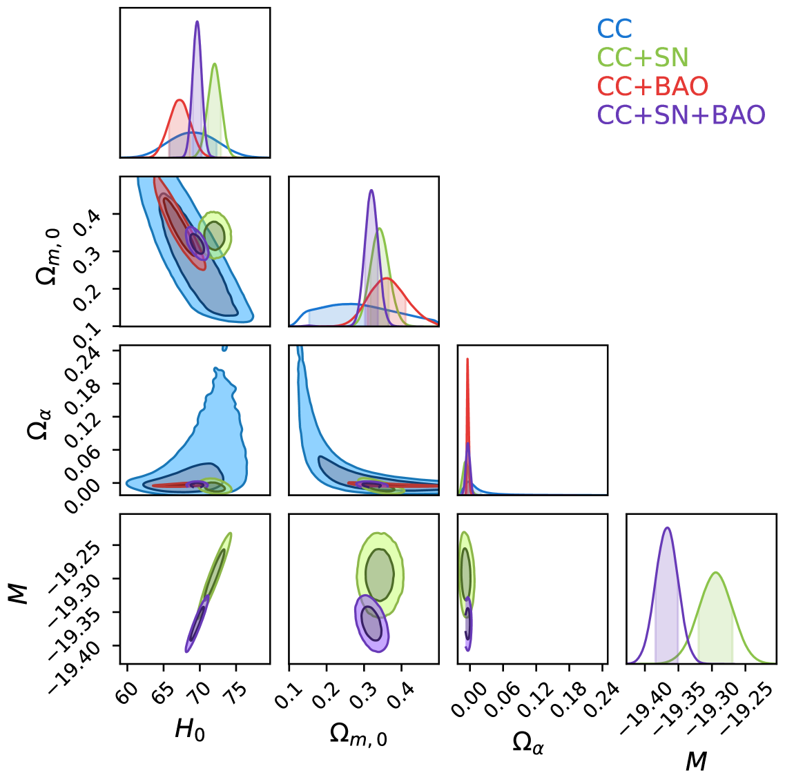
The outputs of the MCMC constraint analysis are shown in Table 1, while the corresponding $\Lambda$CDM fits are contained in Appendix A. One notes that higher Hubble constants are obtained in the quadratic Palatini cases except when BAO data is included. On the other hand, smaller matter density parameters are obtained except for the baseline case. As for the $\Omega_{\alpha}$ parameter, the observational data appears to prefer values that are in the $1-2\sigma$ range as compared with the $\Lambda$CDM value where this parameter is zero. Indeed, for the case where the statistical distance is largest from $\Lambda$CDM, namely for the CC+BAO data set, the statistical criterions give a negative value indicating that the model is slightly preferred, whereas the other cases show a marginal preference for the standard cosmological model.

We consider the case of adding the $H_{0}^{\rm S22}$ prior to all the data sets under consideration in Fig. 2 to assess the consistency of the analyses with this value of the Hubble constant reported in the literature. The introduction of the prior makes the absolute magnitude and Hubble constant anti-correlation more pronuanced while the consistency of the matter density parameter is slightly perturbed. On the other hand, the posterior values of the $\Omega_{\alpha}$ parameter are generically more consistent with $\Lambda$CDM in this scenario.

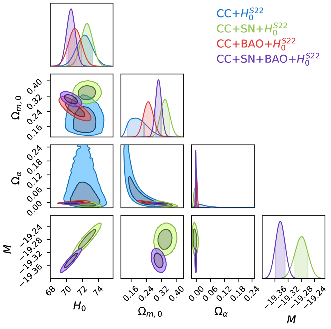
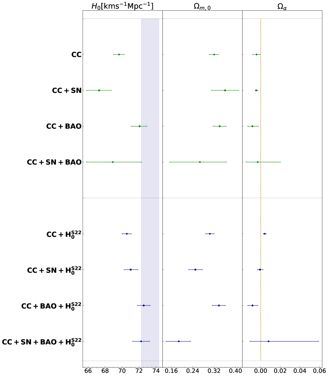
The outputs of the MCMC analyses of the Palatini model for the $H_{0}^{\rm S22}$ prior case are shown in Table 2. Generically, we find higher values of the fits for the Hubble constant, as one would expect, but we also find lower values of the matter density parameters with reasonable uncertainties, which is consistent with how one would expect the cosmology to evolve. On the other hand, the precise fits for the $\Omega_{\alpha}$ parameter are consistent with $\Lambda$CDM but there is a preference for a nontrivial $\Omega_{\alpha}$. By and large the statistical performance of the model against the different data sets remains largely the same. The superior performance of the model for the instance where we consider CC+BAO data set is considered remains the case. The various fits for the model parameters and the different data set combinations are shown in Fig. 3 which contains a whisker plot of the final constraints together with an indicative region for the $H_{0}^{\rm S22}$ prior.

References

- Misner et al. [1973] C. W. Misner, K. S. Thorne, and J. A. Wheeler, Gravitation (W. H. Freeman, San Francisco, 1973).
- Clifton et al. [2012] T. Clifton, P. G. Ferreira, A. Padilla, and C. Skordis, Phys. Rept. 513, 1 (2012), arXiv:1106.2476 [astro-ph.CO] .
- Peebles and Ratra [2003] P. J. E. Peebles and B. Ratra, Rev. Mod. Phys. 75, 559 (2003), arXiv:astro-ph/0207347 .
- Baudis [2016] L. Baudis, J. Phys. G 43, 044001 (2016).
- Bertone et al. [2005] G. Bertone, D. Hooper, and J. Silk, Phys. Rept. 405, 279 (2005), arXiv:hep-ph/0404175 .
- Copeland et al. [2006] E. J. Copeland, M. Sami, and S. Tsujikawa, Int. J. Mod. Phys. D 15, 1753 (2006), arXiv:hep-th/0603057 .
- Weinberg [1989] S. Weinberg, Rev. Mod. Phys. 61, 1 (1989).
- Gaitskell [2004] R. J. Gaitskell, Ann. Rev. Nucl. Part. Sci. 54, 315 (2004).
- Di Bari et al. [2013] P. Di Bari, S. F. King, and A. Merle, Phys. Lett. B 724, 77 (2013), arXiv:1303.6267 [hep-ph] .
- Bennett et al. [1993] C. L. Bennett, N. W. Boggess, E. S. Cheng, M. G. Hauser, T. Kelsall, J. C. Mather, S. H. Moseley, T. L. Murdock, R. A. Shafer, R. F. Silverberg, G. F. Smoot, R. Weiss, and E. L. Wright, Proceedings of the National Academy of Sciences 90, 4766 (1993), https://www.pnas.org/doi/pdf/10.1073/pnas.90.11.4766 .
- Eisenhardt et al. [2020] P. R. M. Eisenhardt, F. Marocco, J. W. Fowler, A. M. Meisner, J. D. Kirkpatrick, N. Garcia, T. H. Jarrett, R. Koontz, E. J. Marchese, S. A. Stanford, D. Caselden, M. C. Cushing, R. M. Cutri, J. K. Faherty, C. R. Gelino, A. H. Gonzalez, A. Mainzer, B. Mobasher, D. J. Schlegel, D. Stern, H. I. Teplitz, and E. L. Wright, The Astrophysical Journal 247, 69 (2020), arXiv:1908.08902 [astro-ph.IM] .
- Eriksen et al. [2007] H. K. Eriksen, A. J. Banday, K. M. Gorski, F. K. Hansen, and P. B. Lilje, Astrophys. J. Lett. 660, L81 (2007), arXiv:astro-ph/0701089 .
- Aghanim et al. [2020a] N. Aghanim et al. (Planck), Astron. Astrophys. 641, A6 (2020a), [Erratum: Astron.Astrophys. 652, C4 (2021)], arXiv:1807.06209 [astro-ph.CO] .
- Perivolaropoulos and Skara [2022] L. Perivolaropoulos and F. Skara, New Astron. Rev. 95, 101659 (2022), arXiv:2105.05208 [astro-ph.CO] .
- Di Valentino et al. [2021a] E. Di Valentino et al., Astropart. Phys. 131, 102606 (2021a), arXiv:2008.11283 [astro-ph.CO] .
- Di Valentino et al. [2021b] E. Di Valentino et al., Astropart. Phys. 131, 102605 (2021b), arXiv:2008.11284 [astro-ph.CO] .
- Di Valentino et al. [2021c] E. Di Valentino et al., Astropart. Phys. 131, 102604 (2021c), arXiv:2008.11285 [astro-ph.CO] .
- Di Valentino et al. [2021d] E. Di Valentino et al., Astropart. Phys. 131, 102607 (2021d), arXiv:2008.11286 [astro-ph.CO] .
- Riess et al. [2019] A. G. Riess, S. Casertano, W. Yuan, L. M. Macri, and D. Scolnic, Astrophys. J. 876, 85 (2019), arXiv:1903.07603 [astro-ph.CO] .
- Anderson et al. [2023] R. I. Anderson, N. W. Koblischke, and L. Eyer, (2023), arXiv:2303.04790 [astro-ph.CO] .
- Wong et al. [2020] K. C. Wong et al., Mon. Not. Roy. Astron. Soc. 498, 1420 (2020), arXiv:1907.04869 [astro-ph.CO] .
- Madhavacheril et al. [2023] M. S. Madhavacheril et al. (ACT), (2023), arXiv:2304.05203 [astro-ph.CO] .
- Schöneberg et al. [2022a] N. Schöneberg, L. Verde, H. Gil-Marín, and S. Brieden, JCAP 11, 039 (2022a), arXiv:2209.14330 [astro-ph.CO] .
- Riess [2019] A. G. Riess, Nature Rev. Phys. 2, 10 (2019), arXiv:2001.03624 [astro-ph.CO] .
- Pesce et al. [2020] D. W. Pesce et al., Astrophys. J. Lett. 891, L1 (2020), arXiv:2001.09213 [astro-ph.CO] .
- de Jaeger et al. [2020] T. de Jaeger, B. E. Stahl, W. Zheng, A. V. Filippenko, A. G. Riess, and L. Galbany, Mon. Not. Roy. Astron. Soc. 496, 3402 (2020), arXiv:2006.03412 [astro-ph.CO] .
- Capozziello et al. [2023] S. Capozziello, G. Sarracino, and A. D. A. M. Spallicci, Phys. Dark Univ. 40, 101201 (2023), arXiv:2302.13671 [astro-ph.CO] .
- Abdalla et al. [2022] E. Abdalla et al., JHEAp 34, 49 (2022), arXiv:2203.06142 [astro-ph.CO] .
- Bernal et al. [2016] J. L. Bernal, L. Verde, and A. G. Riess, JCAP 10, 019 (2016), arXiv:1607.05617 [astro-ph.CO] .
- Sotiriou and Faraoni [2010a] T. P. Sotiriou and V. Faraoni, Rev. Mod. Phys. 82, 451 (2010a), arXiv:0805.1726 [gr-qc] .
- Akrami et al. [2021] Y. Akrami et al. (CANTATA), Modified Gravity and Cosmology: An Update by the CANTATA Network, edited by E. N. Saridakis, R. Lazkoz, V. Salzano, P. Vargas Moniz, S. Capozziello, J. Beltrán Jiménez, M. De Laurentis, and G. J. Olmo (Springer, 2021) arXiv:2105.12582 [gr-qc] .
- Krishnan et al. [2021] C. Krishnan, E. O. Colgáin, M. M. Sheikh-Jabbari, and T. Yang, Phys. Rev. D 103, 103509 (2021), arXiv:2011.02858 [astro-ph.CO] .
- Colgáin et al. [2022] E. O. Colgáin, M. M. Sheikh-Jabbari, R. Solomon, G. Bargiacchi, S. Capozziello, M. G. Dainotti, and D. Stojkovic, Phys. Rev. D 106, L041301 (2022), arXiv:2203.10558 [astro-ph.CO] .
- Malekjani et al. [2023] M. Malekjani, R. M. Conville, E. O. Colgáin, S. Pourojaghi, and M. M. Sheikh-Jabbari, (2023), arXiv:2301.12725 [astro-ph.CO] .
- Ren et al. [2022] X. Ren, S.-F. Yan, Y. Zhao, Y.-F. Cai, and E. N. Saridakis, Astrophys. J. 932, 2 (2022), arXiv:2203.01926 [astro-ph.CO] .
- Dainotti et al. [2021] M. G. Dainotti, B. De Simone, T. Schiavone, G. Montani, E. Rinaldi, and G. Lambiase, Astrophys. J. 912, 150 (2021), arXiv:2103.02117 [astro-ph.CO] .
- Addazi et al. [2022] A. Addazi et al., Prog. Part. Nucl. Phys. 125, 103948 (2022), arXiv:2111.05659 [hep-ph] .
- Schöneberg et al. [2022b] N. Schöneberg, G. Franco Abellán, A. Pérez Sánchez, S. J. Witte, V. Poulin, and J. Lesgourgues, Phys. Rept. 984, 1 (2022b), arXiv:2107.10291 [astro-ph.CO] .
- Anchordoqui [2021] L. A. Anchordoqui, Phys. Rev. D 103, 035025 (2021), arXiv:2010.09715 [hep-ph] .
- Alam et al. [2003] U. Alam, V. Sahni, and A. A. Starobinsky, JCAP 04, 002 (2003), arXiv:astro-ph/0302302 .
- Gariazzo et al. [2022] S. Gariazzo, E. Di Valentino, O. Mena, and R. C. Nunes, Phys. Rev. D 106, 023530 (2022), arXiv:2111.03152 [astro-ph.CO] .
- Piedipalumbo et al. [2023] E. Piedipalumbo, S. Vignolo, P. Feola, and S. Capozziello, Phys. Dark Univ. 42, 101274 (2023), arXiv:2307.02355 [gr-qc] .
- Solà et al. [2017] J. Solà, A. Gómez-Valent, and J. de Cruz Pérez, Astrophys. J. 836, 43 (2017), arXiv:1602.02103 [astro-ph.CO] .
- Akarsu et al. [2023] O. Akarsu, E. Di Valentino, S. Kumar, R. C. Nunes, J. A. Vazquez, and A. Yadav, (2023), arXiv:2307.10899 [astro-ph.CO] .
- Colgáin et al. [2023] E. O. Colgáin, S. Pourojaghi, M. M. Sheikh-Jabbari, and D. Sherwin, (2023), arXiv:2307.16349 [astro-ph.CO] .
- Poulin et al. [2023] V. Poulin, T. L. Smith, and T. Karwal, (2023), arXiv:2302.09032 [astro-ph.CO] .
- Di Valentino et al. [2018] E. Di Valentino, C. Bøehm, E. Hivon, and F. R. Bouchet, Phys. Rev. D 97, 043513 (2018), arXiv:1710.02559 [astro-ph.CO] .
- Jedamzik et al. [2021] K. Jedamzik, L. Pogosian, and G.-B. Zhao, Commun. in Phys. 4, 123 (2021), arXiv:2010.04158 [astro-ph.CO] .
- Escamilla-Rivera et al. [2020] C. Escamilla-Rivera, M. A. C. Quintero, and S. Capozziello, JCAP 03, 008 (2020), arXiv:1910.02788 [astro-ph.CO] .
- Capozziello [2002] S. Capozziello, Int. J. Mod. Phys. D 11, 483 (2002), arXiv:gr-qc/0201033 .
- Capozziello and De Laurentis [2011] S. Capozziello and M. De Laurentis, Phys. Rept. 509, 167 (2011), arXiv:1108.6266 [gr-qc] .
- Nojiri and Odintsov [2011] S. Nojiri and S. D. Odintsov, Phys. Rept. 505, 59 (2011), arXiv:1011.0544 [gr-qc] .
- Nojiri et al. [2017] S. Nojiri, S. D. Odintsov, and V. K. Oikonomou, Phys. Rept. 692, 1 (2017), arXiv:1705.11098 [gr-qc] .
- Olmo [2011] G. J. Olmo, JCAP 10, 018 (2011), arXiv:1101.2841 [gr-qc] .
- Olmo and Singh [2009] G. J. Olmo and P. Singh, JCAP 01, 030 (2009), arXiv:0806.2783 [gr-qc] .
- Szydłowski et al. [2016] M. Szydłowski, A. Stachowski, A. Borowiec, and A. Wojnar, Eur. Phys. J. C 76, 567 (2016), arXiv:1512.04580 [gr-qc] .
- Koivisto [2010] T. S. Koivisto, Phys. Rev. D 82, 044022 (2010), arXiv:1004.4298 [gr-qc] .
- Capozziello et al. [2019] S. Capozziello, R. D’Agostino, and O. Luongo, Gen. Rel. Grav. 51, 2 (2019), arXiv:1806.06385 [gr-qc] .
- Bombacigno and Montani [2019] F. Bombacigno and G. Montani, Eur. Phys. J. C 79, 405 (2019), arXiv:1809.07563 [gr-qc] .
- Roshan and Shojai [2008] M. Roshan and F. Shojai, Phys. Lett. B 668, 238 (2008), arXiv:0809.1272 [gr-qc] .
- Sotiriou [2006] T. P. Sotiriou, Phys. Rev. D 73, 063515 (2006), arXiv:gr-qc/0509029 .
- Camera et al. [2023] S. Camera, S. Capozziello, L. Fatibene, and A. Orizzonte, Eur. Phys. J. Plus 138, 180 (2023), arXiv:2212.13825 [gr-qc] .
- Barragan et al. [2009] C. Barragan, G. J. Olmo, and H. Sanchis-Alepuz, Phys. Rev. D 80, 024016 (2009), arXiv:0907.0318 [gr-qc] .
- Barragan and Olmo [2010] C. Barragan and G. J. Olmo, Phys. Rev. D 82, 084015 (2010), arXiv:1005.4136 [gr-qc] .
- Koivisto [2007] T. Koivisto, Phys. Rev. D 76, 043527 (2007), arXiv:0706.0974 [astro-ph] .
- Uddin et al. [2007] K. Uddin, J. E. Lidsey, and R. Tavakol, Class. Quant. Grav. 24, 3951 (2007), arXiv:0705.0232 [gr-qc] .
- Szydłowski and Stachowski [2018] M. Szydłowski and A. Stachowski, Phys. Rev. D 97, 103524 (2018), arXiv:1712.00822 [gr-qc] .
- de Souza et al. [2013] R. C. de Souza, R. Andre, and G. M. Kremer, Phys. Rev. D 87, 083510 (2013), arXiv:1301.7711 [gr-qc] .
- Bauer and Demir [2011] F. Bauer and D. A. Demir, Phys. Lett. B 698, 425 (2011), arXiv:1012.2900 [hep-ph] .
- Rasanen and Wahlman [2017] S. Rasanen and P. Wahlman, JCAP 11, 047 (2017), arXiv:1709.07853 [astro-ph.CO] .
- Tenkanen [2019] T. Tenkanen, Phys. Rev. D 99, 063528 (2019), arXiv:1901.01794 [astro-ph.CO] .
- Shaposhnikov et al. [2020] M. Shaposhnikov, A. Shkerin, and S. Zell, JCAP 07, 064 (2020), arXiv:2002.07105 [hep-ph] .
- Gialamas et al. [2020] I. D. Gialamas, A. Karam, A. Lykkas, and T. D. Pappas, Phys. Rev. D 102, 063522 (2020), arXiv:2008.06371 [gr-qc] .
- Meng and Wang [2004] X.-H. Meng and P. Wang, Class. Quant. Grav. 21, 2029 (2004), arXiv:gr-qc/0402011 .
- Enckell et al. [2019] V.-M. Enckell, K. Enqvist, S. Rasanen, and L.-P. Wahlman, JCAP 02, 022 (2019), arXiv:1810.05536 [gr-qc] .
- Antoniadis et al. [2018] I. Antoniadis, A. Karam, A. Lykkas, and K. Tamvakis, JCAP 11, 028 (2018), arXiv:1810.10418 [gr-qc] .
- Bostan [2020] N. Bostan, Phys. Lett. B 811, 135954 (2020), arXiv:1907.13235 [gr-qc] .
- Karam et al. [2021a] A. Karam, E. Tomberg, and H. Veermäe, JCAP 06, 023 (2021a), arXiv:2102.02712 [astro-ph.CO] .
- Verner [2021] S. Verner, JCAP 04 (2021), 10.1088/1475-7516/2021/04/001, arXiv:2010.11201 [gr-qc] .
- Dimopoulos and Sánchez López [2021] K. Dimopoulos and S. Sánchez López, Phys. Rev. D 103, 043533 (2021), arXiv:2012.06831 [gr-qc] .
- Dimopoulos et al. [2022] K. Dimopoulos, A. Karam, S. Sánchez López, and E. Tomberg, (2022), arXiv:2206.14117 [gr-qc] .
- Bauer and Demir [2008] F. Bauer and D. A. Demir, Phys. Lett. B 665, 222 (2008), arXiv:0803.2664 [hep-ph] .
- Järv et al. [2020] L. Järv, A. Karam, A. Kozak, A. Lykkas, A. Racioppi, and M. Saal, Phys. Rev. D 102, 044029 (2020), arXiv:2005.14571 [gr-qc] .
- Karam et al. [2021b] A. Karam, S. Karamitsos, and M. Saal, JCAP 10, 068 (2021b), arXiv:2103.01182 [gr-qc] .
- Bostan [2023] N. Bostan, JCAP 02, 063 (2023), arXiv:2209.02434 [astro-ph.CO] .
- Eadkhong et al. [2023] T. Eadkhong, P. Dam-O, P. Channuie, and D. Momeni, Nucl. Phys. B 994, 116289 (2023), arXiv:2303.00572 [gr-qc] .
- Afonso et al. [2017] V. I. Afonso, C. Bejarano, J. Beltran Jimenez, G. J. Olmo, and E. Orazi, Class. Quant. Grav. 34, 235003 (2017), arXiv:1705.03806 [gr-qc] .
- Beltrán Jiménez and Delhom [2019] J. Beltrán Jiménez and A. Delhom, Eur. Phys. J. C 79, 656 (2019), arXiv:1901.08988 [gr-qc] .
- Beltrán Jiménez and Delhom [2020] J. Beltrán Jiménez and A. Delhom, Eur. Phys. J. C 80, 585 (2020), arXiv:2004.11357 [gr-qc] .
- Allemandi et al. [2004a] G. Allemandi, A. Borowiec, and M. Francaviglia, Phys. Rev. D 70, 043524 (2004a), arXiv:hep-th/0403264 .
- Allemandi et al. [2004b] G. Allemandi, A. Borowiec, and M. Francaviglia, Phys. Rev. D 70, 103503 (2004b), arXiv:hep-th/0407090 .
- Olmo et al. [2020] G. J. Olmo, D. Rubiera-Garcia, and A. Wojnar, Phys. Rept. 876, 1 (2020), arXiv:1912.05202 [gr-qc] .
- Allemandi et al. [2005] G. Allemandi, A. Borowiec, M. Francaviglia, and S. D. Odintsov, Phys. Rev. D 72, 063505 (2005), arXiv:gr-qc/0504057 .
- Borowiec et al. [2012] A. Borowiec, M. Kamionka, A. Kurek, and M. Szydlowski, JCAP 02, 027 (2012), arXiv:1109.3420 [gr-qc] .
- Wojnar [2018] A. Wojnar, Eur. Phys. J. C 78, 421 (2018), arXiv:1712.01943 [gr-qc] .
- Gogoi and Goswami [2022] D. J. Gogoi and U. D. Goswami, Int. J. Mod. Phys. D 31, 2250048 (2022), arXiv:2108.01409 [gr-qc] .
- Coumbe [2019] D. Coumbe, Int. J. Mod. Phys. A 34, 31 (2019), arXiv:1910.05629 [gr-qc] .
- Sotiriou and Faraoni [2010b] T. P. Sotiriou and V. Faraoni, Rev. Mod. Phys. 82, 451 (2010b), arXiv:0805.1726 [gr-qc] .
- Borowiec et al. [2016] A. Borowiec, A. Stachowski, M. Szydłowski, and A. Wojnar, JCAP 01, 040 (2016), arXiv:1512.01199 [gr-qc] .
- Stachowski et al. [2017] A. Stachowski, M. Szydłowski, and A. Borowiec, Eur. Phys. J. C 77, 406 (2017), arXiv:1608.03196 [gr-qc] .
- Riess et al. [2022] A. G. Riess et al., Astrophys. J. Lett. 934, L7 (2022), arXiv:2112.04510 [astro-ph.CO] .
- Zhang et al. [2014] C. Zhang, H. Zhang, S. Yuan, T.-J. Zhang, and Y.-C. Sun, Res. Astron. Astrophys. 14, 1221 (2014), arXiv:1207.4541 [astro-ph.CO] .
- Jimenez et al. [2003] R. Jimenez, L. Verde, T. Treu, and D. Stern, Astrophys. J. 593, 622 (2003), arXiv:astro-ph/0302560 .
- Moresco et al. [2016] M. Moresco, L. Pozzetti, A. Cimatti, R. Jimenez, C. Maraston, L. Verde, D. Thomas, A. Citro, R. Tojeiro, and D. Wilkinson, JCAP 05, 014 (2016), arXiv:1601.01701 [astro-ph.CO] .
- Simon et al. [2005] J. Simon, L. Verde, and R. Jimenez, Phys. Rev. D 71, 123001 (2005), arXiv:astro-ph/0412269 .
- Moresco et al. [2012] M. Moresco et al., JCAP 08, 006 (2012), arXiv:1201.3609 [astro-ph.CO] .
- Stern et al. [2010] D. Stern, R. Jimenez, L. Verde, M. Kamionkowski, and S. A. Stanford, JCAP 02, 008 (2010), arXiv:0907.3149 [astro-ph.CO] .
- Moresco [2015] M. Moresco, Mon. Not. Roy. Astron. Soc. 450, L16 (2015), arXiv:1503.01116 [astro-ph.CO] .
- Scolnic et al. [2022] D. Scolnic et al., Astrophys. J. 938, 113 (2022), arXiv:2112.03863 [astro-ph.CO] .
- Conley et al. [2011] A. Conley et al. (SNLS), Astrophys. J. Suppl. 192, 1 (2011), arXiv:1104.1443 [astro-ph.CO] .
- Ross et al. [2015] A. J. Ross, L. Samushia, C. Howlett, W. J. Percival, A. Burden, and M. Manera, Mon. Not. Roy. Astron. Soc. 449, 835 (2015), arXiv:1409.3242 [astro-ph.CO] .
- Beutler et al. [2011] F. Beutler, C. Blake, M. Colless, D. H. Jones, L. Staveley-Smith, L. Campbell, Q. Parker, W. Saunders, and F. Watson, Mon. Not. Roy. Astron. Soc. 416, 3017 (2011), arXiv:1106.3366 [astro-ph.CO] .
- Anderson et al. [2014] L. Anderson et al. (BOSS), Mon. Not. Roy. Astron. Soc. 441, 24 (2014), arXiv:1312.4877 [astro-ph.CO] .
- Zhao et al. [2019] G.-B. Zhao et al., Mon. Not. Roy. Astron. Soc. 482, 3497 (2019), arXiv:1801.03043 [astro-ph.CO] .
- Alam et al. [2017] S. Alam et al. (BOSS), Mon. Not. Roy. Astron. Soc. 470, 2617 (2017), arXiv:1607.03155 [astro-ph.CO] .
- Aghanim et al. [2020b] N. Aghanim et al. (Planck), Astron. Astrophys. 641, A6 (2020b), [Erratum: Astron.Astrophys. 652, C4 (2021)], arXiv:1807.06209 [astro-ph.CO] .
- Akaike [1974] H. Akaike, IEEE Transactions on Automatic Control 19, 716 (1974).
- Pinto et al. [2018] P. Pinto, L. Del Vecchio, L. Fatibene, and M. Ferraris, JCAP 11, 044 (2018), arXiv:1807.00397 [gr-qc] .
- Olmo [2005] G. J. Olmo, Phys. Rev. Lett. 95, 261102 (2005), arXiv:gr-qc/0505101 .
- Toniato et al. [2020] J. D. Toniato, D. C. Rodrigues, and A. Wojnar, Phys. Rev. D 101, 064050 (2020), arXiv:1912.12234 [gr-qc] .
- Hernandez-Arboleda et al. [2022] A. Hernandez-Arboleda, D. C. Rodrigues, and A. Wojnar, (2022), arXiv:2204.03762 [astro-ph.GA] .
- Hernandez-Arboleda et al. [2023] A. Hernandez-Arboleda, D. C. Rodrigues, J. D. Toniato, and A. Wojnar, in Metric-Affine Frameworks for Gravity 2022 (2023) arXiv:2306.04475 [gr-qc] .
- Kozak and Wojnar [2023a] A. Kozak and A. Wojnar, Phys. Rev. D 108, 044055 (2023a), arXiv:2303.17213 [gr-qc] .
- Kozak and Wojnar [2023b] A. Kozak and A. Wojnar, (2023b), arXiv:2308.01784 [gr-qc] .
- Baker et al. [2015] T. Baker, D. Psaltis, and C. Skordis, Astrophys. J. 802, 63 (2015), arXiv:1412.3455 [astro-ph.CO] .