Cosmological implications of baryon acoustic oscillation (BAO) measurements
Abstract
We derive constraints on cosmological parameters and tests of dark energy models from the combination of baryon acoustic oscillation (BAO) measurements with cosmic microwave background (CMB) data and a recent reanalysis of Type Ia supernova (SN) data. In particular, we take advantage of high-precision BAO measurements from galaxy clustering and the Lyman- forest (LyaF) in the SDSS-III Baryon Oscillation Spectroscopic Survey (BOSS). Treating the BAO scale as an uncalibrated standard ruler, BAO data alone yield a high confidence detection of dark energy; in combination with the CMB angular acoustic scale they further imply a nearly flat universe. Adding the CMB-calibrated physical scale of the sound horizon, the combination of BAO and SN data into an “inverse distance ladder” yields a measurement of , with 1.7% precision. This measurement assumes standard pre-recombination physics but is insensitive to assumptions about dark energy or space curvature, so agreement with CMB-based estimates that assume a flat CDM cosmology is an important corroboration of this minimal cosmological model. For constant dark energy (), our BAO+SN+CMB combination yields matter density and curvature . When we allow more general forms of evolving dark energy, the BAO+SN+CMB parameter constraints are always consistent with flat CDM values at . While the overall of model fits is satisfactory, the LyaF BAO measurements are in moderate () tension with model predictions. Models with early dark energy that tracks the dominant energy component at high redshift remain consistent with our expansion history constraints, and they yield a higher and lower matter clustering amplitude, improving agreement with some low redshift observations. Expansion history alone yields an upper limit on the summed mass of neutrino species, (95% confidence), improving to if we include the lensing signal in the Planck CMB power spectrum. In a flat CDM model that allows extra relativistic species, our data combination yields ; while the LyaF BAO data prefer higher when excluding galaxy BAO, the galaxy BAO alone favor . When structure growth is extrapolated forward from the CMB to low redshift, standard dark energy models constrained by our data predict a level of matter clustering that is high compared to most, but not all, observational estimates.
I Introduction
Acoustic oscillations that propagate in the pre-recombination universe imprint a characteristic scale in the clustering of matter, providing a cosmological “standard ruler” that can be measured in the power spectrum of cosmic microwave background (CMB) anisotropies and in maps of large-scale structure at lower redshifts Sakharov66 ; Peebles70 ; Sunyaev70 ; Blake03 ; Seo03 . While distance scale measurements with Type Ia supernovae (SNIa) are calibrated against systems in the local Hubble flow Hamuy96 ; Riess98 ; Perlmutter99 , the baryon acoustic oscillation (BAO) scale is computed from first principles, using physical parameters (such as the radiation, matter, and baryon densities) that are well constrained by CMB data. The difference between absolute and relative measurements, the sharpening of BAO precision with increasing redshift, and the entirely independent systematic uncertainties make BAO and SNe highly complementary tools for measuring the cosmic expansion history and testing dark energy models. In spectroscopic surveys, BAO measurements in the line-of-sight dimension allow direct determinations of the expansion rate , in addition to the constraints from transverse clustering on the comoving angular diameter distance in a flat spatial metric.111We use the notation to refer to the comoving angular diameter distance, which is also referred to in the literature as the proper motion distance Hogg99 . This notation avoids confusion with the proper angular diameter distance .
The first clear detections of low-redshift BAO Cole05 ; Eisenstein05 came from galaxy clustering analyses of the Two Degree Field Galaxy Redshift Survey (2dFGRS, Colless01 ) and the luminous red galaxy (LRG, Eisenstein01 ) sample of the Sloan Digital Sky Survey (SDSS, York00 ). Analyses of the final 2dFGRS and SDSS-II redshift surveys yielded BAO distance measurements with aggregate precision of 2.7% at Percival10 , subsequently sharpened to 1.9% Padmanabhan12 by application of reconstruction methods Eisenstein07 that suppress non-linear degradation of the BAO feature. The WiggleZ survey Drinkwater10 pushed BAO measurements to higher redshifts, achieving 3.8% aggregate precision from galaxies in the redshift range Blake11 . The Six Degree Field Galaxy Survey (6dFGS, Jones09 ) took advantage of its 17,000 deg2 sky coverage to provide a BAO measurement at low redshift, achieving 4.5% precision at Beutler11 . A recent reanalysis that applies reconstruction to the main galaxy sample Strauss02 of SDSS-II obtained 3.8% precision at Ross:2014qpa , in a sky area that has minimal () overlap with 6dFGS.
The Baryon Oscillation Spectroscopic Survey (BOSS, Dawson13 ) of SDSS-III Eisenstein11 has two defining objectives: to measure the BAO distance scale with one-percent precision from a redshift survey of 1.5 million luminous galaxies at , and to make the first BAO measurement at using 3-dimensional structure in the Ly forest absorption towards a dense grid of 160,000 high-redshift quasars. This paper explores the cosmological implications of BAO measurements from the BOSS Data Release 11 (DR11) data sample, in combination with a variety of other cosmological data. The measurements themselves, including detailed discussion of statistical uncertainties and extensive tests for systematic errors, have been presented in previous papers. For the galaxy survey, Anderson14 report a 1.4% measurement of and a 3.5% measurement of at (1 uncertainties, with a correlation coefficient of ), and a 2.0% measurement of from lower redshift BOSS galaxies at . The precision at is 1.0%. For the Ly forest (often abbreviated as LyaF below), we combine constraints from the auto-correlation function, with 2.6% precision on and 5.4% precision on Delubac14 , and the quasar-forest cross-correlation, with precision of 3.3% on and 3.7% on FontRibera14 , both at an effective redshift . While some cosmological analysis appears in these papers, the combination of galaxy and Ly forest BAO measurements and the addition of other data allow us to constrain broader classes of cosmological models and to search for deviations from standard assumptions.
The combination of BAO measurements with precise CMB measurements from the Planck and WMAP satellites already yields tight constraints on the parameters of the CDM cosmological model (inflationary cold dark matter with a cosmological constant and zero space curvature222Throughout the paper, the notation CDM refers to spatially flat models; cosmological constant models allowing non-zero curvature are denoted CDM.) and on one-parameter extensions of this model that allow, e.g., non-zero curvature, an evolving dark energy density, or a cosmologically significant neutrino mass PlanckXVI . We also take advantage of another major recent advance, a comprehensive reassessment of the SNIa distance scale by Betoule14 using data from the 3-year Supernova Legacy Survey Conley11 and SDSS-II Supernova Survey Frieman08 ; Sako14 samples and additional data at low and high redshifts. We will examine the consistency of the BAO and SNIa results for relative distances and the constraints on that emerge from an “inverse distance ladder” that combines the two data sets, in essence using SNIa to transfer the absolute calibration of the BAO scale from the intermediate redshifts where it is precisely measured down to . Our primary focus will be on the cosmological parameter constraints and model tests that come from combining the BAO and SNIa data with Planck CMB data.333We use the Planck 2013 data, which were publicly available at the time of our analysis and paper submission. Because best-fit parameter values from the Planck 2015 data are similar to those from the Planck 2013 data Planck2015XIII , we expect that using the 2015 data would make little difference to our results, though with some modest improvements in parameter uncertainties. We will present analyses that use the Planck 2015 data in concert with BOSS DR12 BAO measurements in future work. When fitting models to these data, we will also examine their predictions for observable measures of structure growth and compare the results to inferences from weak lensing, clusters, redshift-space distortions, and the 1-d Ly power spectrum. The interplay of BAO, CMB, and SNIa constraints, and the more general interplay between measurements of expansion history and structure growth, are reviewed at length by Weinberg13 , along with detailed introductions to the methods themselves. In particular, Section 4 of Weinberg13 provides a thorough description of the BAO method and its motivation.
Section II describes the basic methodology of our analysis, including the relevant underlying equations, and reviews the BAO, CMB, and SN measurements that we adopt for our constraints, concluding with variants of “BAO Hubble diagrams” that illustrate our qualitative results. Section III presents the constraints obtainable by assuming that the BAO scale is a standard ruler independent of redshift without computing its physical scale; in particular, we demonstrate that galaxy and LyaF BAO alone yield a convincing detection of dark energy and that addition of the angular scale of the CMB acoustic peaks requires a nearly flat universe if dark energy is a cosmological constant. Section IV presents our inverse distance ladder determination of , which assumes standard recombination physics but does not assume a specific dark energy model or a flat universe. Section V describes our constraints on the parameters of standard dark energy models, while Section VI considers models that allow early dark energy, decaying dark matter, cosmologically significant neutrino mass, or extra relativistic species. We compare the predictions of our BAO+SN+CMB constrained models to observational estimates of matter clustering in Section VII and summarize our overall conclusions in Section VIII.
II Methodology, Models and Data Sets
II.1 Methodology
A homogenenous and isotropic cosmological model is specified by the curvature parameter entering the Friedman-Robertson-Walker metric
| (1) |
which governs conversion between radial and transverse distances, and by the evolution of . In General Relativity (GR), this evolution is governed by the Friedmann equation Friedman22 , which can be written in the form
| (2) |
where is the Hubble parameter, is the total energy density (radiation + matter + dark energy), and the subscript 0 denotes the present day (). We define the density parameter of component by the ratio
| (3) |
and the curvature parameter
| (4) |
where the sum is over all matter and energy components and for a flat () universe. Density parameters and always refer to values at unless a dependence on or is written explicitly, e.g., . We will frequently refer to the Hubble constant through the dimensionless ratio . The dimensionless quantity is proportional to the physical density of component at the present day.
Given the curvature parameter and from the Friedmann equation, the comoving angular diameter distance can be computed as
| (5) |
where the line-of-sight comoving distance is
| (6) |
where
| (7) |
Positive corresponds to negative . We do not use the small approximation of equation (5) in our calculations, but we provide it here to illustrate that for small non-zero curvature the change in distance is linear in and quadratic in .
Curvature affects both through its influence on and through the geometrical factor in equation (5). The luminosity distance (relevant to supernovae) is .
The energy components considered in our models are pressureless (cold) dark matter, baryons, radiation, neutrinos, and dark energy. The densities of CDM and baryons scale as ; we refer to the density parameter of these two components together as . The energy density of neutrinos with non-zero mass scales like radiation at early times and like matter at late times, with
| (8) |
where both CMB temperature and neutrino temperature scale inversely with scale factor, and the neutrino temperature is given by , where accounts for small amount of heating of neutrinos due to electron-positron annihilation. The sum in the above expression is over neutrino species with masses . The integral is given by
| (9) |
and must be evaluated numerically. For massless neutrinos , while in the limit of very massive neutrinos (for ; here is the Riemann function), i.e., scaling proportionally with so that neutrinos behave like pressureless matter. When we refer to the matter density parameter , we include the contributions of radiation (which is small compared to the uncertainties in ) and neutrinos (which are non-relativistic at ), so that . Following the Planck Collaboration PlanckXVI , we adopt eV with one massive and two massless neutrino species in all models except the one referred to as CDM, where it is a free parameter. The default implies including massless species and excluding them. The effect of finite neutrino temperature at is a very small relative effect. The adopted values are close to the minimum value allowed by neutrino oscillation experiments.
We consider a variety of models for the evolution of the energy density or equation-of-state parameter . Table 1 summarizes the primary models discussed in the paper, though we consider some additional special cases in Section VI. CDM represents a flat universe with a cosmological constant (). CDM extends this model to allow non-zero . CDM adopts a flat universe and constant , and CDM generalizes to non-zero . CDM and CDM allow to evolve linearly with , . PolyCDM adopts a quadratic polynomial form for and allows non-zero space curvature, to provide a highly flexible description of the effects of dark energy at low redshift. Finally, Slow Roll Dark Energy is an example of a one-parameter evolving- model, based on a quadratic dark energy potential.
We focus in this paper on parameter constraints and model tests from measurements of cosmic distances and expansion rates, which we refer to collectively as “expansion history” or “geometric” constraints. We briefly consider comparisons to measurements of low-redshift matter clustering in Section VII. In this framework, the crucial roles of CMB anisotropy measurements are to constrain the parameters (mainly and ) that determine the BAO scale and to determine the angular diameter distance to the redshift of recombination. For most of our analyses, this approach allows us to use a highly compressed summary of CMB constraints, discussed in Section II.3 below, and to compute parameter constraints with a simple and fast Markov Chain Monte Carlo (MCMC) code that computes expansion rates and distances from the Friedmann equation. The code is publicly available with data used in this paper at https://github.com/slosar/april.
| Name | Friedmann equation () | Curvature | Section(s) |
| CDM | no | III-V | |
| CDM | yes | III-V | |
| CDM | no | V | |
| CDM | yes | V | |
| CDM | no | V | |
| Slow Roll Dark Energy | no | V | |
| CDM | yes | IV-V | |
| PolyCDM | yes444with Gaussian prior | IV | |
| Early Dark Energy | See relevant section. | no | VI.1 |
| Decaying Dark Matter | See relevant section. | no | VI.2 |
| CDM | free neutrino mass () | no | VI.3 |
| CDM | non-standard radiation component ( ) | no | VI.4 |
| Tuned Oscillation | See relevant section. | no | VI.5 |
II.2 BAO data
The BAO data in this work are summarized in Table 2 and more extensively discussed below.
| Name | Redshift | ||||
|---|---|---|---|---|---|
| 6dFGS | 0.106 | – | – | – | |
| MGS | 0.15 | – | – | – | |
| BOSS LOWZ Sample | 0.32 | – | – | – | |
| BOSS CMASS Sample | 0.57 | – | |||
| LyaF auto-correlation | 2.34 | – | |||
| LyaF-QSO cross correlation | 2.36 | – | |||
| Combined LyaF | 2.34 | – |
The robustness of BAO measurements arises from the fact that a sharp feature in the correlation function (or an oscillatory feature in the power spectrum) cannot be readily mimicked by systematics, whether observational or astrophysical, as these should be agnostic about the BAO scale and hence smooth over the relevant part of the correlation function (or power spectrum). In most current analyses, the BAO scale is determined by adopting a fiducial cosmological model that translates angular and redshift separations to comoving distances but allowing the location of the BAO feature itself to shift relative to the fiducial model expectation. One then determines the likelihood of obtaining the observed two-point correlation function or power spectrum as a function of the BAO offsets, while marginalizing over nuisance parameters. These nuisance parameters characterize “broad-band” physical or observational effects that smoothly change the shape or amplitude of the underlying correlation function or power spectrum, such as scale-dependent bias of galaxies or the LyaF, or distortions caused by continuum fitting or by variations in star-galaxy separation. In an isotropic fit, the measurement is encoded in the parameter, the ratio of the measured BAO scale to that predicted by the fiducial model. In an anisotropic analysis, one separately constrains and , the ratios perpendicular and parallel to the line of sight. In real surveys the errors on and are significantly correlated for a given redshift slice, but they are typically uncorrelated across different redshift slices. While the values of are referred to a specified fiducial model, the corresponding physical BAO scales are insensitive to the choice of fiducial model within a reasonable range.
The BAO scale is set by the radius of the sound horizon at the drag epoch when photons and baryons decouple,
| (10) |
where the sound speed in the photon-baryon fluid is . A precise prediction of the BAO signal requires a full Boltzmann code computation, but for reasonable variations about a fiducial model the ratio of BAO scales is given accurately by the ratio of values computed from the integral (10). Thus, a measurement of from clustering at redshift constrains the ratio of the comoving angular diameter distance to the sound horizon:
| (11) |
A measurement of constrains the Hubble parameter , which we convert to an analogous quantity:
| (12) |
with
| (13) |
An isotropic BAO analysis measures some effective combination of these two distances. If redshift-space distortions are weak, which is a good approximation for luminous galaxy surveys after reconstruction but not for the LyaF, then the constrained quantity is the volume averaged distance
| (14) |
with
| (15) |
There are different conventions in use for defining , which differ at the 1-2% level, but ratios of for different cosmologies are independent of the convention provided one is consistent throughout. In this work we adopt the CAMB convention for , i.e., the value that is reported by the linear perturbations code CAMBLewis00 . In practice, we use the numerically calibrated approximation
| (16) |
This approximation is accurate to 0.021% for a standard radiation background with , , and values of and within of values derived by Planck. It supersedes a somewhat less accurate (but still sufficiently accurate) approximation from Anderson14 (their eq. 55). Note that , and a 0.5 (1.0) eV neutrino mass changes by () for fixed . For neutrino masses in the range allowed by current cosmological constraints, the CMB constrains rather than because neutrinos remain relativistic at recombination, even though they are non-relativistic at . For the case of extra relativistic species, a useful fitting formula is
| (17) |
which is accurate to 0.119% if we restrict to neutrino masses in the range and . Increasing by unity decreases by about 3.2%.
For CDM models (with , ) constrained by Planck, Mpc. This 0.4% uncertainty is only slightly larger for CDM, CDM, or even CDM (see Table 1 for cosmological model definitions), because the relevant quantities and are constrained by the relative heights of the acoustic peaks, not by their angular locations. The inference of matter energy densities from peak heights thus depends on correct understanding of physics in the pre-recombination epoch, where curvature and dark energy are negligible in any of these models.
BAO measurements constrain cosmological parameters through their influence on , their influence on via the Friedmann equation, and their influence on via equation (5). For standard models, the 0.4% error on from Planck is small compared to current BAO measurement errors, so the constraints come mainly through and . From the Friedmann equation, we see that is directly sensitive to the total energy density at redshift , while constrains an effective average of the energy density and is also sensitive to curvature.
Measurements in Table 2 are reported in terms of , , and , using the convention of equation (10). Expressed in these terms, the results are independent of the fiducial cosmologies assumed in the individual analysis papers. Note that some of the referenced papers quote values of rather than , differing by a factor . An anisotropic analysis yields anti-correlated errors on and , and the correlation coefficients are reported in Table 2. Each sample spans a range of redshift, and the quoted effective redshift is usually weighted by statistical contribution to the BAO measurement. Because redshift-space positions are scaled to comoving coordinates based on a fiducial cosmological model, and BAO measurements are obtained as ratios relative to that fiducial model, the values of the effective redshift in Table 2 can be treated as exact, e.g., one should compare the BOSS CMASS numbers to model predictions computed at
II.2.1 Galaxy BAO Measurements
The most precise BAO measurements to date come from analyses of the BOSS DR11 galaxy sample by Anderson14 . BOSS uses the same telescope Gunn06 as the original SDSS, with spectrographs Smee13 that were substantially upgraded to improve throughput and increase multiplexing (from 640 fibers per plate to 1000). Redshift completeness for the primary BOSS sample is nearly 99%, with typical redshift uncertainty of a few tens of Bolton12 . The DR11 sample has a footprint of 8377 deg2, compared to 10,500 deg2 expected for the final BOSS galaxy sample to appear in DR12.
BOSS targets two distinct samples of luminous galaxies selected by different flux and color cuts Dawson13 : CMASS, designed to approximate a constant threshold in galaxy stellar mass in the range , and LOWZ, which provides roughly three times the density of the SDSS-II LRG sample in the range . Analysis of both samples incorporates reconstruction Eisenstein07 ; Padmanabhan12 to sharpen the BAO peak by partly reversing non-linear effects, thus improving measurement precision. For CMASS, we use results of the anisotropic analysis by Anderson14 , which yields (1.4% precision) and (3.5% precision) with anti-correlated errors ().
The LOWZ sample does not have sufficient statistical power for a robust anisotropic analysis, so we use the measurement of at (discussed in detail by Tojeiro14 ). We have not included results from the SDSS-II LRG or WiggleZ surveys cited in the introduction because these partly overlap the BOSS volume and are not statistically independent. We do include results of a new analysis Ross:2014qpa that uses reconstruction to achieve a 3.8% measurement from the SDSS main galaxy sample (MGS) at effective redshift , which should be nearly independent of the BOSS LOWZ measurement. We also include the 6dFGS measurement of (4.5% precision) at . Because the 6dFGS BAO detection is of moderate statistical significance and we do not have a full surface for it, we truncate its contributions at to guard against non-Gaussian tails of the error distribution. In practice the 6dFGS measurement carries little statistical weight in our constraints. These galaxy BAO measurements are listed in the first four lines of Table 2.
II.2.2 BOSS Ly forest BAO Measurements
The BAO scale was first measured at higher redshift () from the auto-correlation of the Ly forest fluctuations in the spectra of high-redshift quasars from BOSS DR9 (Busca13 ,Slosar13 ,Kirkby13 ) following the pioneering work of measuring 3D fluctuations in the forest 2011JCAP…09..001S . Here we use the results from Delubac14 , who present an improved measurement using roughly twice as many quasar spectra from BOSS DR11. The DR11 quasar catalog will be made publicly available simultaneously with the DR12 catalog in 2015. The catalog construction is similar to that of the DR10 quasar catalog described by 2014A&A…563A..54P . The BOSS quasar selection criteria are described by 2012ApJS..199….3R and the background methodology papers 2012ApJ…749…41B ; 2011ApJ…743..125K ; Richards09 ; 2010A&A…523A..14Y .
The measurement of LyaF BAO peak positions is marginalized over parameters describing broad-band distortion of the correlation function using the methodology of Kirkby13 . Because of the low effective bias factor of the LyaF, redshift-space distortion strongly enhances the BAO peak in the line-of-sight direction. The measurement of is therefore more precise (3.1%) than that of (5.8%), as seen in line 5 of Table 2. The errors of these two measurements are anti-correlated, with , and the optimally measured combination is determined with a precision of . While the overall signal-to-noise ratio of the BAO measurement is high, the detection significance for transverse separations () is only moderate, as one can see in Figure 3 of Delubac14 .
At the same redshift, BAO have also been measured in the cross-correlation of the Ly forest with the density of quasars in BOSS DR11 FontRibera14 . While the number of quasar-pixel pairs is much lower than the number of pixel-pixel pairs in the auto-correlation function, the clustering signal is much stronger because of the high bias factor of quasars. For the same reason, redshift-space distortion is much weaker in the cross-correlation, and in this case the measurement precision is comparable for (3.7%) and for (3.3%), (line 6 of Table 2). The higher precision of the transverse measurement makes the cross-correlation measurement an especially valuable complement to the auto-correlation measurement.
Even though these results are derived from the same volume, we can consider them as independent because their uncertainties are not dominated by cosmic variance. They are dominated instead by the combination of noise in the spectra and sparse sampling of the structure in the survey volume, both of which affect the auto-correlation and cross-correlation almost independently. A number of tests using mock catalogs and several analysis procedures are presented in Delubac14 , finding good agreement between error estimates from the likelihood function and from the variance in mock catalogs. This independence allows us to add the surfaces from both publications, which are publicly available at http://darkmatter.ps.uci.edu/baofit/. While we use these two surfaces separately, the last line of Table 2 lists the and constraints from the combined measurement, with respective precision of 3.2% and 2.2% and a correlation coefficient .
We caution that BAO measurement from LyaF data is a relatively new field, pioneered entirely by BOSS, in contrast to the now mature subject of galaxy BAO measurement, which has been studied both observationally and theoretically by many groups. Delubac14 present numerous tests using mock catalogs and different analysis procedures, finding good agreement between error estimates from the likelihood surface and from mock catalog variance and identifying no systematic effects that are comparable to the statistical errors. However, the analysis uses only 100 mock catalogs, limiting the external tests of the tails of the error distribution. The systematics and error estimation of the cross-correlation measurement have also been less thoroughly examined than those of the auto-correlation measurement, though continuing investigations within the BOSS collaboration find good agreement with the errors and covariances reported in the publications above. On the theoretical side, Pontzen14 and Gontcho14 have examined the potential impact of UV background fluctuations on LyaF BAO measurement, finding effects that are much smaller than the current statistical errors.
We anticipate significant improvements in the LyaF analyses of the Data Release 12 sample, thanks to the larger data set and ongoing work on broadband distortion modeling, larger mock catalog samples, and spectro-photometric calibration. For the current paper, we adopt the BAO likelihood surfaces as reported in FontRibera14 and Delubac14 .
II.3 Cosmic Microwave Background Data
In this paper we focus on constraints on the expansion history of the homogeneous cosmological model. For this purpose, we compress the Cosmic Microwave Background (CMB) measurements to the variables governing this expansion history. This approach greatly simplifies the required computations, allowing us to fit complex models that have a simple solution to the Friedmann equation without the need to numerically solve for the evolution of perturbations. It is also physically illuminating, making clear what relevant quantities the CMB determines and distinguishing expansion history constraints from those that depend on the evolution of clustering. For some models or special cases we use more complete CMB results obtained by running the industry-standard cosmomc 2002PhRvD..66j3511L or by relying on the publicly available Planck MCMC chains.555http://wiki.cosmos.esa.int/planckpla/index.php/ Cosmological_Parameters
The CMB plays two distinct but important roles in our analysis. First, we treat the CMB as a “BAO experiment” at redshift , measuring the angular scale of the sound horizon at very high redshift. Here we ignore the small dependence of the last-scattering redshift on cosmological parameters and the fact that the relevant scale for the CMB is rather than the drag redshift that sets the BAO scale in low-redshift structure. We have checked that both approximations are valid to around for the case of BAO and Planck data and the CDM model. In its second important role, the CMB calibrates the absolute length of the BAO ruler through its determination of and .
Inspired by the existence of well-known degeneracies in CMB data 1999MNRAS.304…75E ; 2002PhRvD..66f3007K ; Wang13 , we compress the CMB measurements into three variables: , and . The mean vector and the covariance matrix are used to describe the CMB constraints by a simple Gaussian likelihood. In order to calibrate these variables, we rely on the publicly available Planck chains. In particular, we use the base_Alens chains with the planck_lowl_lowLike dataset corresponding to the Planck dataset with low- WMAP polarization (referred to in this paper as Planck+WP). We find that the data vector
| (18) |
can be described by a Gaussian likelihood with mean
| (19) |
and covariance
| (20) |
The fractional diagonal errors on , , and are 1.5%, 1.9%, and 0.06%, respectively. We similarly compress the WMAP 9-yr data into
| (21) |
and covariance
| (22) |
For reference in interpreting the cosmological constraints from CMB+BAO data, especially in Section VI below, note that the contributions to accumulate over a wide range of redshift, with 14%, 25%, 38%, 47%, 69%, 88%, and 99% of the integral in equation (6) coming from redshifts , 1.0, 2.0, 3.0, 10, 50, and 640, respectively.
The base_Alens model corresponds to the basic flat CDM cosmology with explicit marginalisation over the foreground lensing potential. Our decision to use the flat model was intentional, since we found that in curved models there is significant non-Gaussian correlation of and with curvature. Because our BAO data inevitably collapse more complex models to nearly flat ones, use of the flat data is more appropriate. We have tested the data compression in a couple of simple cases by comparing results of BAO+CMB data to cosmomc chains and found less than differences in best-fit parameter values between using compressed and full chains. The residual differences are driven by the fact that our compressed likelihood attempts to extract purely geometric information from the CMB data (for example, values of and are different at roughly the same level between chains that marginalise over lensing potential and those that do not). For BAO-only data combinations the results are completely consistent.
Throughout the paper, we refer to the constraints represented by equations (18)-(20) simply as “Planck” (although they also include information from WMAP polarization measurements). In Section III we treat the CMB as a BAO experiment measuring , but we eliminate its calibration of the absolute BAO scale by artificially blowing up the errors on and ; we denote this case as “Planck ”. Conversely, in Section IV we use the CMB information on and to set the size of our standard ruler but omit the information by artificially inflating its errors; we denote this case as “”. When we use a full Planck chain instead of the compressed information, we adopt the notation “Planck (full)” and specify what additional parameters (such as , , or tensor-to-scalar ratio ) are being varied in the chain.
If one assumes a flat universe, a cosmological constant (), standard relativistic background (), and minimal neutrino mass (), then the CMB data summarized by equations (18)-(20) also provide a precise constraint on the Hubble parameter , and thus on , , and . At various points in the paper we refer to a “fiducial” Planck CDM model for which we adopt , , and , which are the best fit parameters for “Planck+WP” combination as cited in the Table 2 of PlanckXVI . The CMB constraints on and become much weaker if one allows or , so for more general models BAO data or other constraints are needed to restore high precision on cosmological parameters.
II.4 Supernova Data
A comprehensive set of relative luminosity distances of 740 SNIa was presented in Betoule14 , based on a joint calibration and training set of the SDSS-II Supernova Survey Sako14 and the Supernova Legacy Survey (SNLS) 3-year data set Conley11 . The 374 supernovae from SDSS-II and 239 from SNLS were combined with 118 nearby supernovae from Contreras10 ; Hicken09 ; Jha06 ; Altavilla04 ; Riess99 ; Hamuy96 and nine high-redshift supernovae discovered and studied by HST Riess07 . We use this set, dubbed Joint Light-curve Analysis (JLA), rather than the Union 2.1 compilation of Suzuki2012 because of the demonstrated improvement in calibration and corresponding reduction in systematic uncertainties presented in Betoule14 .
While Betoule14 also provide a full cosmomc module and a covariance matrix in relevant parameters, we here instead use their compressed representation of relative distance constraints due to conceptual simplicity and a drastic increase in computational speed when combining with other cosmology probes. The compressed information consists of a piece-wise linear function fit over 30 bins (leading to 31 nodes) spaced evenly in (to minimum ) with a covariance matrix that includes all of the systematics from the original analysis. SNIa constrain relative distances, so the remaining marginalization required to use this compressed respresentation in a comological analysis is over the fiducial absolute magnitude of a SNIa, . In Section IV we also utilize a similar compression of the Union 2.1 SN data set, which we have constructed in analogous fashion.
II.5 Visualizing the BAO Constraints
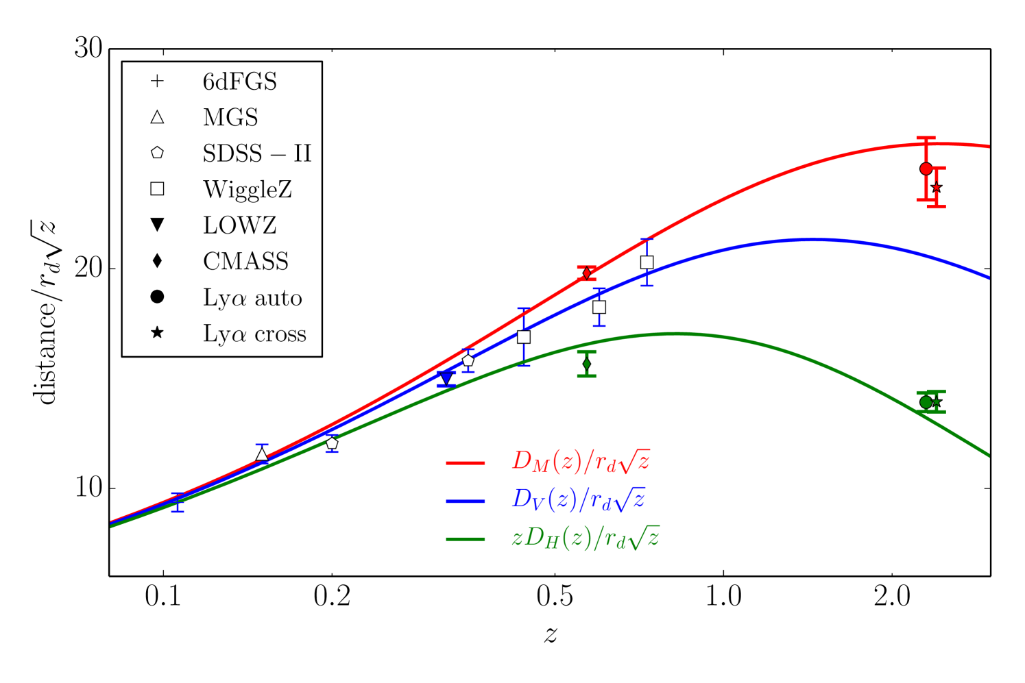
Figure 1 shows the “Hubble diagram” (distance vs. redshift) from a variety of recent BAO measurements of , , or ; these three quantities converge at low redshift. In addition to the data listed in Table 2, we show measurements from the DR7 data set of SDSS-II by Percival10 and from the WiggleZ survey by Blake11 , which are not included in our cosmological analysis because they are not independent of the (more precise) BOSS measurements in similar redshift ranges. Curves represent the predictions of the fiducial Planck CDM model, whose parameters are determined independently of the BAO measurements but depend on the assumptions of a flat universe and a cosmological constant. Overall, there is impressively good agreement between the CMB-constrained CDM model and the BAO measurements, especially as no parameters have been adjusted in light of the BAO data. However, there is noticeable tension between the Planck CDM model and the LyaF BAO measurements.

Figure 2 displays a subset of these BAO measurements with scalings that elucidate their physical content. In the upper panel, we plot , which is the proper velocity between two objects with a constant comoving separation of 1 Mpc. This quantity is declining in a decelerating universe and increasing in an accelerating universe. We set the -axis to be , which makes a straight line of slope in an Einstein-de Sitter () model. For the transverse BAO measurements in the lower panel, we plot , chosen so that a constant (horizontal) line in the plot would produce the same constant line in this panel, assuming a flat Universe. This quantity would decrease monotonically in a non-accelerating flat cosmology. The quantities in both the upper and lower panels approach as approaches zero, independent of other cosmological parameters. We convert the BOSS LOWZ and MGS measurements of to in the lower panel assuming the fiducial Planck CDM parameters; this is a robust approximation because all acceptable cosmologies produce similar scaling at these low redshifts. Note that the and measurements from a given data set (i.e., at a particular redshift) are covariant, in the sense that the points on these panels are anti-correlated (see Table 2). For example, if at were scattered upward by a statistical fluctuation, then the point in the lower panel would be scattered downward.
As discussed below in Section IV, the galaxy BAO and JLA supernova data can be combined to yield an “inverse distance ladder” measurement of , which utilizes the CMB measurements of and but no other CMB information. This value of is robust to a wide range of assumptions about dark energy evolution and space curvature, although it does assume a standard radiation background for the calculation of . We plot the resulting determination of as the open square in both panels.
The grey swath in both panels of Figure 2 represents the 1 region for the fiducial Planck CDM model, with the top panel clearly showing the transition from deceleration to acceleration at . Formally, we are scaling both panels by , so that the comparison of the BAO data points to the CMB prediction is invariant to changes in the sound horizon. The galaxy BAO measurements of from BOSS and MGS are in excellent agreement with the predictions of this model (as are the other measurements shown previously in Fig. 1), and the combination of BAO and SNe yields an value in excellent agreement with this model’s prediction. The expansion rate from CMASS is high compared to the model prediction, at moderate significance. Compared to Planck, the best-fit value of from the 9-year WMAP analysis WMAP9 is lower, 0.143 vs. 0.137, implying lower and slightly higher for a CDM model. The model using these best-fit parameters, shown by the dashed lines, agrees better with the CMASS measurement but is in tension with the distance data, especially the CMASS value of .
The Ly forest measurements are much more difficult to reconcile with the CDM model: compared to the Planck curve, the LyaF BAO is low and is high. It is important to keep the error anti-correlation in mind when assessing significance — if fluctuates up then will fluctuate down, which tends to reduce the tension relative to the CMB. However, our subseqent analyses (and those already reported by Delubac14 ) will show that the discrepancy is significant at the level. The dotted curves show predictions of cosmological models with or . While changing curvature or the dark energy equation-of-state can improve agreement with some of the data points, it worsens agreement with other data points, and on the whole (as demonstrated quantitatively in Section V) such variations do not noticeably improve the fit to the combined CMB, BAO, and SN data.
Not plotted in Figure 2 is the value of that comes from the angular acoustic scale in the CMB. Connecting the acoustic scale measured in CMB anisotropy to that measured in large-scale structure does require model assumptions about structure formation at the recombination epoch. However, it would be difficult to move the relative calibration significantly without making substantial changes to the CMB damping tail, which is already well constrained by observations. Using the ratio of in equation (19) and Mpc, we find at with percent level accuracy, a factor of two larger than any of the low-redshift values in Figure 2. On their own, the BAO data in Figure 2 clearly favor a universe that transitions from deceleration at to acceleration at low redshifts, and this evidence becomes overwhelming if one imagines the corresponding CMB measurements off the far left of the plot. We quantify these points in the following section.
It is tempting to consider a flat cosmology with a constant as an alternative model of these data Melia12 . Note that although this form of occurs in coasting (empty) cosmologies in general relativity, those models have open curvature and hence a sharply different . But even for the flat model, the data are not consistent with a constant , first because the increase in from to is statistically significant, and second because of the factor of two change of this quantity relative to that inferred from the CMB angular acoustic scale. The change from to is more significant than the plot indicates because the data points are correlated; this occurs because the value results from normalizing the SNe distances with the BAO measurements. We measure the ratio of the values, , to be from the combination of BAO and SNe datasets, a 5.5 rejection of a constant hypothesis and an indication of the strength of the SNe data in detecting the low-redshift accelerating expansion.
III BAO as an uncalibrated ruler
III.1 Convincing Detection of dark energy from BAO data alone
For quantitative contraints, we start by considering BAO data alone with the simple assumption that the BAO scale is a standard comoving ruler, whose length is independent of redshift and orientation but is not necessarily the value computed using CMB parameter constraints. A similar analysis has been presented in 2013MNRAS.436.1674A . In this case, a simple dimensional analysis shows that in addition to fractional densities in cosmic components, one can constrain the dimensionless quantity .
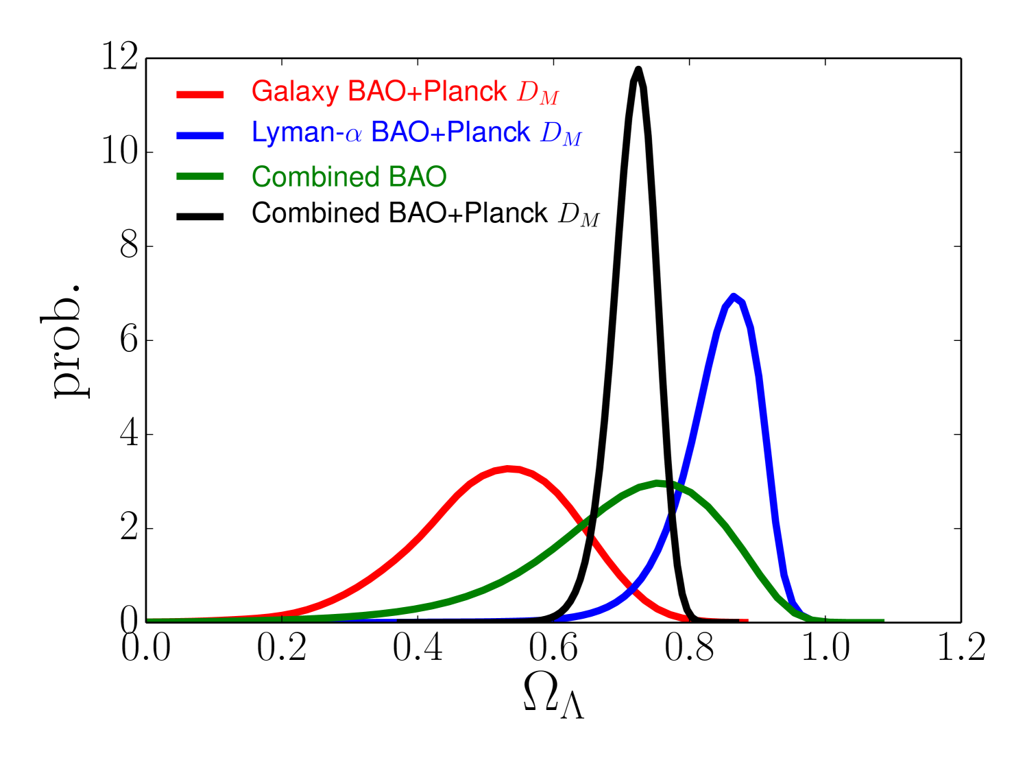
Figure 3 presents constraints on relevant quantities in CDM models, which assume that dark energy is a cosmological constant but allow and arbitrary . The combination of galaxy and LyaF BAO measurements yields a marginalised constraint of at 99.7% confidence, implying a detection of dark energy from BAO alone without CMB data.
These constraints become much tighter if we assume that the CMB is measuring the same acoustic scale, functioning as an additional BAO experiment at a much higher redshift. As discussed in Section II.3, we implement this case by retaining the high-precision CMB measurement of but drastically inflating (by a factor of 100) the CMB errors on and , so that the value of itself remains effectively unknown. Combining the CMB measurement with galaxy or LyaF BAO alone yields a strong detection of non-zero , but with different central values reflecting the tensions already discussed in Section II.5 and examined further in Sections V–VI. Combining all three measurements yields a marginalised (at 68% confidence, with reasonably Gaussian errors), implying preference for a low-density universe dominated by dark energy. The dimensionless quantity is determined with 1.6% precision. Most importantly, this data combination also requires a nearly flat universe, with a total density determined to 1.5% and consistent with the critical density. Thus, with the minimal assumption that the BAO scale is a standard ruler, these data provide strong support for the standard cosmological model.

III.2 External calibration of
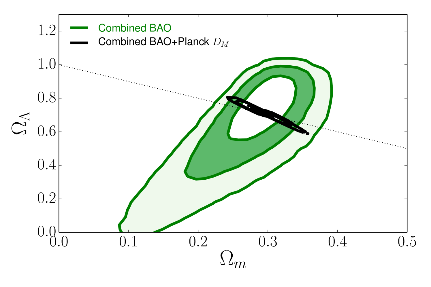
We proceed further by computing the sound horizon scale from the standard physics of the pre-recombination universe but adopting empirical constraints external to the CMB. In particular, we adopt a prior on the baryon density of determined from big bang nucleosynthesis (BBN) and the observed primordial deuterium abundance Cooke14 , and we assume a standard relativistic background (, ). For any values of and the Hubble parameter that arise in our MCMC chain, we can then compute the value of from equation (16). Compared to the previous section, the addition of the physical scale allows us to convert the measured value of into a measurement of the dimensional parameter . In practice, we derive constraints in a separate MCMC run where, instead of a flat prior on , we have a flat prior on and the above prior on . We also fix the curvature parameter to zero. Results are presented in Figure 4. The red (galaxy BAO) and blue (LyaF BAO) contours in this figure use no CMB information at all, but they do assume a spatially flat universe in contrast to Figure 3.
The point of this exercise is the following. The homogeneous part of the minimal CDM model has just two adjustable parameters, and , which matches the two degrees of freedom offered by a measurement of anisotropic BAO at a single redshift. (The weak BBN prior is required to fix the magnitude of , but it does not affect the expansion history.) One can therefore get meaningful constraints from either galaxy BAO or LyaF BAO alone, though this is no longer true if one allows non-zero curvature and therefore introduces a third parameter. There is substantial degeneracy for either measurement individually, but both are generally compatible with standard values of these parameters. The tension of the LyaF BAO with the Planck CDM model manifests itself here as a best fit at relatively low matter density and high Hubble parameter. Combining the galaxy and LyaF measurements produces a precise measurement of both and the Hubble parameter coming from BAO alone, independent of CMB data. In combination, we find and (68% confidence). The small black ellipse in Figure 4 shows the Planck constraints for CDM, computed from full Planck chains, which are in excellent agreement with the region allowed by the joint BAO measurements.

IV BAO, SNIa, and the Inverse Distance Ladder
The traditional route to measuring the Hubble constant is built on a distance ladder anchored in the nearby Universe: stellar distances to galaxies within Mpc are used to calibrate secondary indicators, and these in turn are used to measure distances to galaxies “in the Hubble flow,” i.e., far enough away that peculiar velocities are a sub-dominant source of uncertainty when inferring Freedman10 . The most powerful implementations of this program in recent years have used Cepheid variables — calibrated by direct parallax, by distance estimates to the LMC, or by the maser distance to NGC 4258 — to determine distances to host galaxies of SNIa, which are the most precise of the available secondary distance indicators Riess11 ; Freedman12 ; Humphreys13 .
Because the BAO scale can be computed in absolute units from basic underlying physics, the combination of BAO with SNIa allows a measurement of via an “inverse distance ladder,” anchored at intermediate redshift. The BOSS BAO data provide absolute values of at and at with precision of 2.0% and 1.4%, respectively. The JLA SNIa sample provides a high-precision relative distance scale, which transfers the BAO measurement down to low redshift, where is simply the slope of the distance-redshift relation. Equivalently, this procedure calibrates the absolute magnitude scale of SNIa using BAO distances instead of the Cepheid distance scale. Although the extrapolation from the BAO redshifts to low redshifts depends on the dark energy model, the SNIa relative distance scale is precisely measured over a well sampled redshift interval which includes the BAO redshifts, so this extrapolation introduces practically no uncertainty even when the dark energy model is extremely flexible. CMB data enter the inverse distance ladder by constraining the values of and and thus allowing computation of the sound horizon scale .

Figure 5 provides a conceptual illustration of this approach, zeroing in on the portion of the Hubble diagram. Filled points show from the CMASS, LOWZ, MGS, and 6dFGS BAO measurements, where for illustrative purposes only we have converted the latter three measurements from to using Planck CDM parameters. The error bars on these points include the 0.4% uncertainty in arising from the uncertainties in the Planck determination of and , but this is a small contribution to the error budget. Crosses show the binned SNIa distance measurements, with the best absolute magnitude calibration from the joint BAO+SNIa fit. We caution that systematic effects introduce error correlations across redshift bins in the SNIa data, which are accounted for in our full analysis. To allow flexibility in the dark energy model, we adopt the PolyCDM parameterization described in Section II.1, imposing a loose Gaussian prior to suppress high curvature models that are clearly inconsistent with the CMB. Thin green curves in Figure 5 show for ten PolyCDM models that have relative to the best-fit model, selected from the MCMC chains described below. The intercept of these curves at is the value of . While low-redshift BAO measurements like those of 6dFGS and MGS incur minimal uncertainty from the extrapolation to , the statistical error is necessarily large because of the limited volume at low . It is evident from Figure 5 that using SNIa to transfer intermediate redshift BAO measurements to the local Universe yields a much more precise determination of than using only low-redshift BAO measurements, even allowing for great flexibility in the dark energy model.
To compute our constraints, we adopt the and constraints from CMASS BAO (including covariance), the constraints from LOWZ, MGS, and 6dFGS BAO, the compressed JLA SNIa data set with its full covariance matrix, and an constraint from Planck (see Section II.3). Marginalizing over the PolyCDM parameters yields , a 1.7% measurement. Even if we include the CMB angular diameter distance at its full precision, our central value and error bar on change negligibly because the flexibility of the PolyCDM model effectively decouples low- and high-redshift information.
As a by-product of our measurement, we determine the absolute luminosity of a fiducial SNIa to be mag. Here we define a fiducial SNIa as having SALT2 (as retrained in Betoule14 ) light-curve width and color parameters and and having exploded in a galaxy with a stellar mass
Our best-fit and its uncertainty are shown by the open square and error bar in Figures 2 and 5. To characterize the sources of error, we have repeated our analyses after multiplying either the CMB, SN, or BAO covariance matrix by a factor of ten (and thus reducing errors by ). Reducing the CMB errors, so that they yield an essentially perfect determination of , makes almost no difference to our error, because the 0.4% uncertainty in is already small. Reducing either the SNIa or BAO errors shrinks the error by approximately a factor of two, indicating that the BAO measurement uncertainties and the SNIa measurement uncertainties make comparable contributions to our error budget; the errors add (roughly) linearly rather than in quadrature because both measurements constrain the redshift evolution in our joint fit. If we replace PolyCDM with CDM in our analysis, substituting a different but still highly flexible dark energy model, the derived value of drops by less than and the error bar is essentially unchanged. If we instead fix the dark energy model to CDM, the central value and error bar are again nearly unchanged, because with the dense sampling provided by SNe the extrapolation from the BAO redshifts down to is also only a small source of uncertainty. To test sensitivity to the SN data set, we constructed a compressed description of the Union 2.1 compilation Suzuki2012 analogous to that of the JLA compilation; substituting Union 2.1 for JLA makes negligible difference to our best-fit while increasing the error bar by about 30% (see Table 3). Finally, if we substitute the WMAP9 constraints on and for the Planck constraints, the central decreases by 0.5% (to ) and the error bar grows by 8% (to ).
To summarize, this 1.7% determination of is robust to details of our analysis, with the error dominated by the BAO and SNIa measurement uncertainties. The key assumptions behind this method are (a) standard matter and radiation content, with three species of light neutrinos, and (b) no unrecognized systematics at the level of our statistical errors in the CMB determinations of and , in the BAO measurements, or in the SNIa measurements used to tie them to . Note that the SNIa covariance matrix already incorporates the detailed systematic error budget of Betoule14 . The measurement systematics are arguably smaller than those that affect the traditional distance ladder. Thus, with the caveat that it assumes a standard matter and radiation content, this measurement of is more precise and probably more robust than current distance-ladder measurements.
Non-standard radiation backgrounds remain a topic of intense cosmological investigation, and a convincing mismatch between determinations from the forward and inverse distance ladders could be a distinctive signature of non-standard physics that alters . We can express our constraint in a more model-independent form as
| (23) |
Raising from 3.046 to 4.0 would increase our central value of to (eq. 17, but see further discussion in Section VI.4).
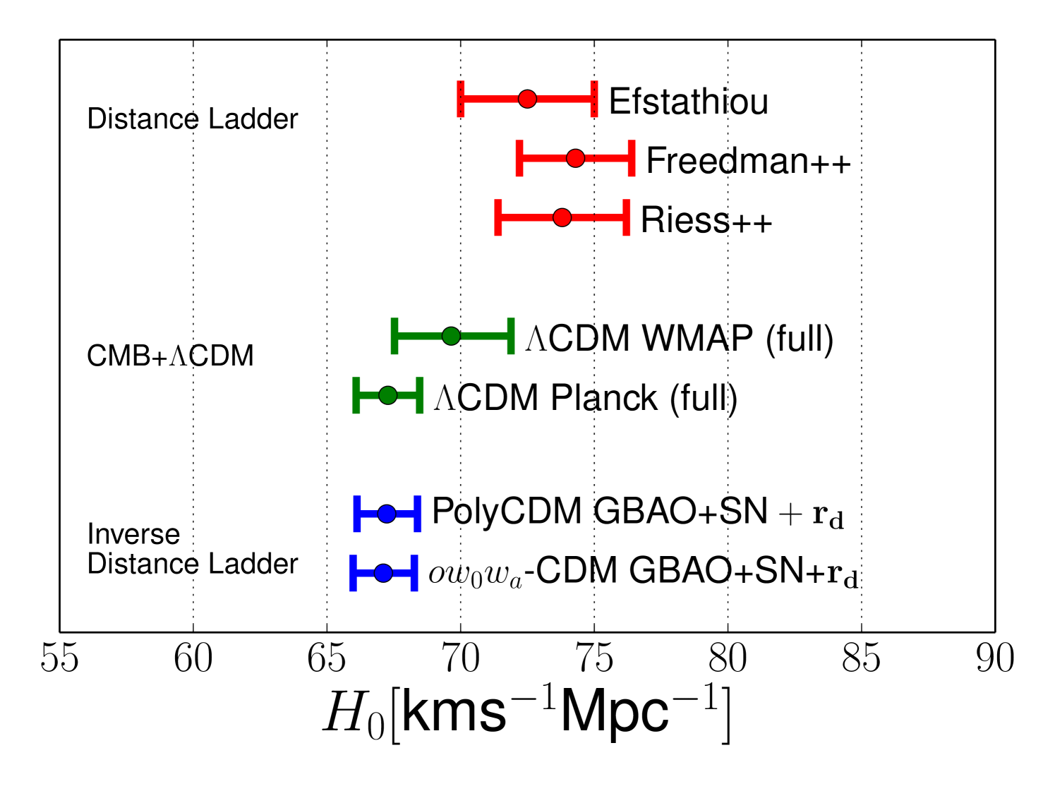
Figure 6 compares our determination to several other values from the literature. The lower two points show our results using either the PolyCDM model or the CDM model. The top three points show recent distance-ladder determinations from Riess et al. Riess11 , Freedman et al. Freedman12 , and a reanalysis of the Riess et al. data set by Efstathiou14 . There is mild () tension between these determinations and our value. The central two points show the values of inferred from Planck or WMAP CMB data assuming a flat CDM model, with values and uncertainties taken from the MCMC chains provided by the Planck collaboration. These inferences of are much more model dependent than our inverse distance ladder measurement; with the CDM or PolyCDM dark energy models the errors on from CMB data alone increase by more than order of magnitude because of the CMB geometric degeneracy. Consistency of these values is therefore a consistency test for the CDM model, which it passes here with flying colors.
| Combination | Model | |
|---|---|---|
| Galaxy BAO + SN + | PolyCDM | |
| Galaxy BAO + SN + | CDM | |
| Galaxy BAO + Union SN + | PolyCDM | |
| Galaxy BAO + Union SN + | CDM |
Our results can be compared to those of several other recent analyses. Cheng14 determine from a collection of BAO data sets using the Planck-calibrated value of . They do not incorporate SNIa, but they assume a flat CDM model, which allows them to obtain a tight constraint . Cuesta14 carry out a more directly comparable inverse distance ladder measurement with essentially the same data sets but cosmological models that are 1-parameter extensions of CDM, finding for either CDM or CDM. 2014arXiv1409.6217H carry out a rather different analysis that uses age measurements for early-type galaxies to provide an absolute timescale. In combination with BAO and SNIa, they then constrain the acoustic oscillation scale independent of CMB data or early universe physics. Their result, which assumes an CDM cosmology, can be cast in a form similar to ours, ; the agreement implies that their stellar evolution age scale is consistent with the scale implied by early-universe BAO physics. As an determination, our analysis makes much more general assumptions about dark energy than these other analyses, but it yields a consistent result. It is also notable that our value of agrees with the value of inferred from a median-statistics analysis of direct distance ladder estimates circa 2001 (Gott01 , see Chen11 for a 2011 update).
From Figure 5, it is visually evident that the relative distance scales implied by our BAO and SN are in fairly good agreement. We have converted SN luminosity distances to comoving angular diameter distances with , a relation that holds in any metric theory of gravity (see section 4.2 of Lampeitl10 and references therein). As a quantitative consistency test, we refit the PolyCDM model with an additional free parameter that artificially modifies the luminosity distance by , finding . This result is consistent with the expected at , but there is a mild tension because the SN data are in good agreement with CDM predictions while the ratio of between the CMASS and LOWZ samples is somewhat higher than expected in CDM.
V Constraints on Dark Energy Models
We now turn to constraints on dark energy and space curvature from the combination of BAO, CMB, and SNIa data. In this section, we consider models with standard matter and radiation content, including three neutrino species with the minimal allowed mass (although the cosmological differences between and are negligible relative to current measurement errors). In Section VI, we will consider models that allow dynamically significant neutrino mass, extra relativistic species, dark matter that decays into radiation, or “early” dark energy that is dynamically non-negligible even at high redshifts.
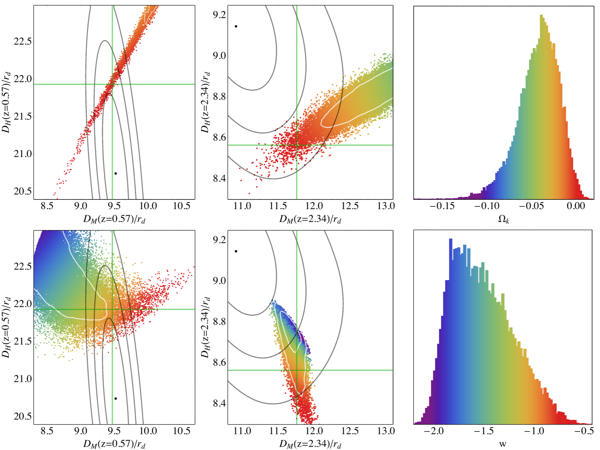
To set the scene, Figure 7 compares the predictions of models constrained by CMB data to the BOSS BAO constraints on and at and , from CMASS galaxies and the LyaF, respectively. Black dots mark best-fit values of , and contours are shown at 6.18, and 11.83 (coverage fractions of 68%, 95%, and 99.7% for a 2-d Gaussian). The top row shows results for CDM models, which assume a constant dark energy density but allow non-zero space curvature. Here we have taken models from the Planck Collaboration MCMC chains, based on the combination of Planck, WMAP polarization, and ACT/SPT data. The upper right panel shows the one-dimensional PDF for the curvature parameter based on the CMB data alone. Each point in the left and middle panels represents a model from the chains, color-coded by the value of on the scale in the right panel. The green cross-hairs mark the predicted from the flat CDM model that best fits the CMB data alone. This model lies just outside the 68% contour for CMASS, but it is discrepant at with the LyaF measurements, as remarked already by Delubac14 . When the flatness assumption is dropped, both the galaxy and LyaF BAO data strongly prefer close to zero, firmly ruling out the slightly closed () models that are allowed by the CMB alone.
The bottom row shows results for CDM models, which assume a flat universe but allow a constant equation-of-state parameter for dark energy. The CMB data alone are consistent with a wide range of values, and they are generally better fit with . However, the combination with CMASS BAO data sharply limits the acceptable range of , favoring values close to (a cosmological constant). The fit to the LyaF BAO results could be significantly improved by going to , but this change would be inconsistent with the CMASS measurements. This example illustrates a general theme of our results: parameter changes that improve agreement with the LyaF BAO measurements usually run afoul of the galaxy BAO measurements.
More quantitative constraints appear in Figure 8 and Table 4. We begin with CDM and continue to the progressively more flexible models described in Table 1. For CMB data, we now use the compression of Planck or WMAP9 constraints described in Section II.3.
We include all of the BAO data listed in Table 2. Omitting the LyaF BAO data makes almost no difference to the central values or error bars on model parameters, though it has a significant impact on goodness-of-fit as we discuss later.
 |
 |
 |
 |
 |
 |
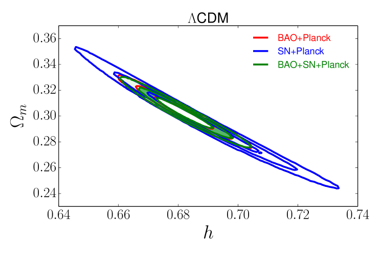
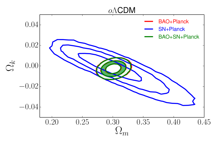
For CDM and CDM, the combination of Planck CMB constraints and BAO is remarkably powerful, a point already emphasized by PlanckXVI . Adding SN data makes negligible difference to the parameter constraints of these models; SN+Planck constraints have nearly identical central values to BAO+Planck, but larger errors. In CDM, substituting BAO+SN+WMAP9 for BAO+SN+Planck has a tiny effect, shifting to with a small compensating shift in . Figure 8 illustrates the extremely tight curvature constraint that comes from combining CMB and BAO data: for CDM we find using Planck CMB or using WMAP9.
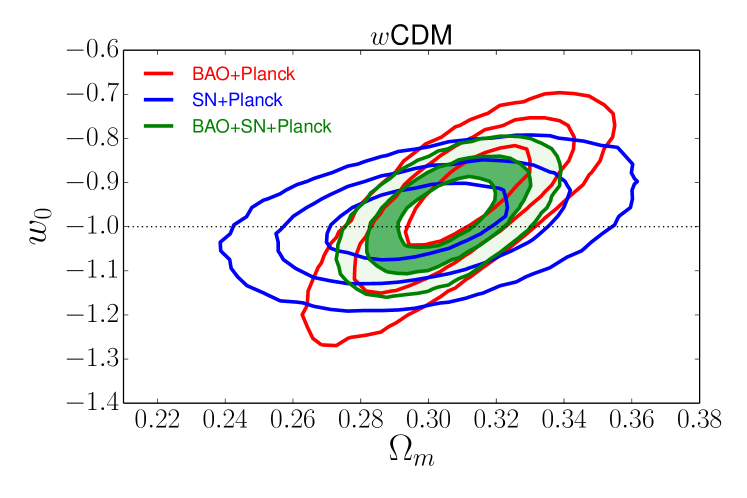
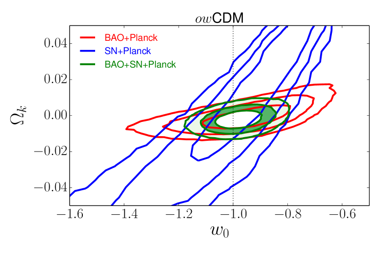
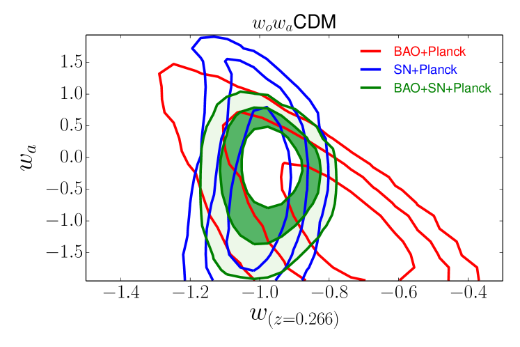
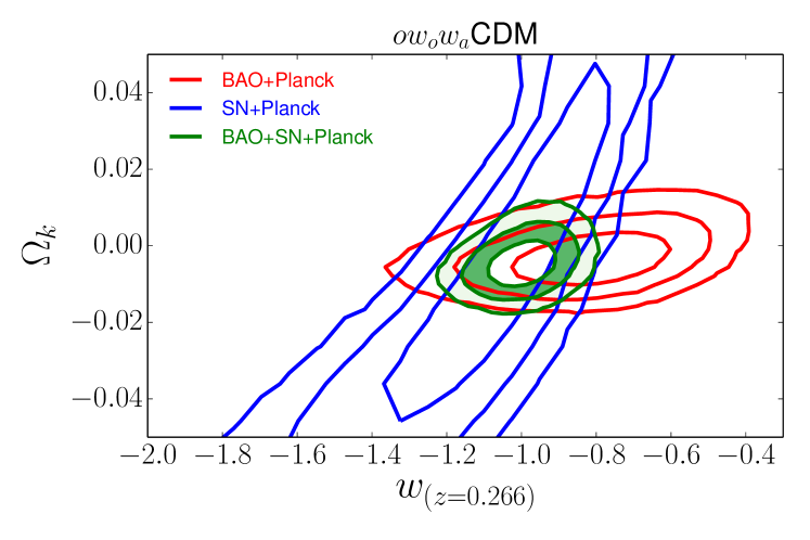
Supernovae play a much more important role in models that allow , as their high precision relative distance measurements provide strong constraints on low-redshift acceleration. For both CDM and CDM, SN+Planck and BAO+Planck constraints are perfectly consistent but complementary, and the combination of all three data sets provides much tighter error bars than any pairwise combination. For CDM we find . For CDM the curvature constraint from BAO is particularly important, lifting the degeneracy between and that arises for SN+CMB alone; we find and . Substituting WMAP9 for Planck again produces only slight shifts to central values and a minor increase of error bars.
Even with these powerful BAO, SN, and CMB data sets, constraining the evolution of is difficult. The constraint on the evolution parameter from BAO+SN+Planck is in CDM and weakens to in CDM. Both results are consistent with constant , but they allow order unity changes of at . This data combination still provides a good constraint on the value of at a “pivot” redshift where it is uncorrelated with (determined specifically for CDMfor BAO+SN+Planck combiations): in CDM and in CDM.
We note that the degradation of our ability to constrain the evolution of the equation of state is not accompanied with significant degradation in our ability to measure the curvature of space: the constraint on curvature remains tight even when allowing an evolving equation of state, .
By decoupling the time dependence of from its present-day value, the model allows flexible evolution of the dark energy density. Adopting a particular form for the dark energy potential reduces this freedom, and one can construct physically motivated models that have evolving dark energy but do not require an additional free parameter to describe it. Gott2011 advocate an interesting example of this model class, in which dark energy is a slowly rolling scalar field with a potential, analogous to the inflaton of chaotic inflation models. Gott2011 show that this model yields and therefore Slepian2014
| (24) | |||||
where the approximation is first-order in .
| Model | Data | ||||||
|---|---|---|---|---|---|---|---|
| CDM | BAO+Planck | 0.303 (8) | 0.0223 (3) | 0.682 (7) | – | – | – |
| CDM | SN+Planck | 0.295 (16) | 0.0224 (3) | 0.688 (13) | – | – | – |
| CDM | BAO+SN+Planck | 0.302 (8) | 0.0223 (3) | 0.682 (6) | – | – | – |
| CDM | BAO+SN+WMAP | 0.300 (8) | 0.0224 (5) | 0.681 (7) | – | – | – |
| CDM | BAO+Planck | 0.301 (8) | 0.0225 (3) | 0.679 (7) | -0.003 (3) | – | – |
| CDM | SN+Planck | 0.30 (4) | 0.0224 (4) | 0.68 (4) | -0.002 (10) | – | – |
| CDM | BAO+SN+Planck | 0.301 (8) | 0.0225 (3) | 0.679 (7) | -0.003 (3) | – | – |
| CDM | BAO+SN+WMAP | 0.295 (9) | 0.0226 (5) | 0.677 (8) | -0.004 (4) | – | – |
| CDM | BAO+Planck | 0.311 (13) | 0.0225 (3) | 0.669 (17) | – | -0.94 (8) | – |
| CDM | SN+Planck | 0.298 (18) | 0.0225 (4) | 0.685 (17) | – | -0.99 (6) | – |
| CDM | BAO+SN+Planck | 0.305 (10) | 0.0224 (3) | 0.676 (11) | – | -0.97 (5) | – |
| CDM | BAO+SN+WMAP | 0.303 (10) | 0.0225 (5) | 0.674 (12) | – | -0.96 (6) | – |
| CDM | BAO+Planck | 0.308 (17) | 0.0225 (4) | 0.671 (19) | -0.001 (4) | -0.95 (11) | – |
| CDM | SN+Planck | 0.28 (8) | 0.0225 (4) | 0.73 (11) | 0.01 (3) | -0.97 (18) | – |
| CDM | BAO+SN+Planck | 0.303 (10) | 0.0225 (4) | 0.676 (11) | -0.002 (3) | -0.98 (6) | – |
| CDM | BAO+SN+WMAP | 0.299 (11) | 0.0227 (5) | 0.671 (12) | -0.004 (4) | -0.96 (6) | – |
| CDM | BAO+Planck | 0.34 (3) | 0.0224 (3) | 0.639 (25) | – | -0.58 (24) | -1.0 (6) |
| CDM | SN+Planck | 0.292 (23) | 0.0224 (4) | 0.693 (24) | – | -0.90 (16) | -0.5 (8) |
| CDM | BAO+SN+Planck | 0.307 (11) | 0.0223 (3) | 0.676 (11) | – | -0.93 (11) | -0.2 (4) |
| CDM | BAO+SN+WMAP | 0.305 (11) | 0.0224 (5) | 0.674 (12) | – | -0.93 (11) | -0.2 (5) |
| CDM | BAO+Planck | 0.34 (3) | 0.0225 (4) | 0.640 (25) | -0.003 (4) | -0.57 (23) | -1.1 (6) |
| CDM | SN+Planck | 0.29 (8) | 0.0225 (4) | 0.72 (11) | 0.01 (3) | -0.94 (21) | -0.3 (9) |
| CDM | BAO+SN+Planck | 0.307 (11) | 0.0225 (4) | 0.673 (11) | -0.005 (4) | -0.87 (12) | -0.6 (6) |
| CDM | BAO+SN+WMAP | 0.302 (11) | 0.0227 (5) | 0.670 (12) | -0.006 (5) | -0.88 (11) | -0.5 (5) |
| SlowRDE | BAO+SN+Planck | 0.307 (10) | 0.0224 (3) | 0.676 (11) | – | -0.95 (7) | – |
| Suzuki et al 2012 Suzuki2012 | … | … | ||||
|---|---|---|---|---|---|---|
| BAO+PLANCK | ||||||
| BAO+SN+PLANCK | ||||||
Figure 9 presents parameter constraints for the slow roll dark energy scenario in a flat universe, a model that has the same number of parameters as CDM. BAO and SN both contribute to the constraints of the joint fit, which yields , , and . Results for this scenario are thus consistent with CDM but allow small departures from .
A striking feature of Table 4 is that the best-fit parameter values barely shift as additional freedom is added to the models. For the BAO+SN+Planck combination, the best-fit values range from 0.301 to 0.307 and the best-fit values from 0.676 to 0.682, while combinations with WMAP9 favor just slightly lower values of and . More importantly, models that allow dark energy evolution are all consistent with constant at , and is consistent with zero at in all cases that allow curvature. The fact that models with additional freedom remain consistent with CDM is a substantial argument in favor of this minimal model.
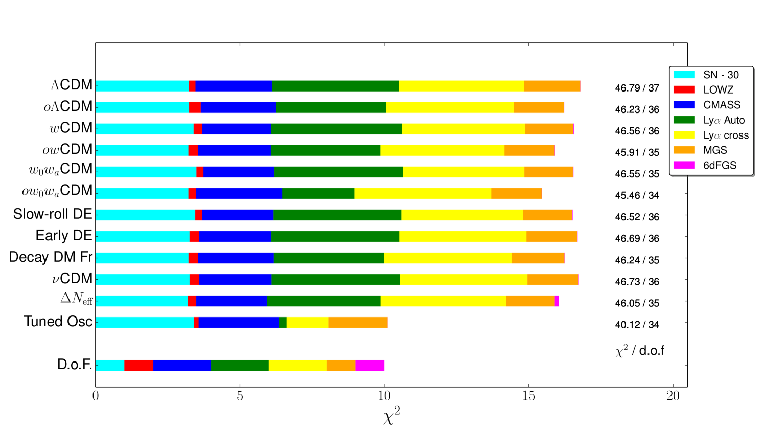
Figure 10 illustrates the goodness-of-fit for the models in Table 4, and for additional models discussed below in Section VI. For the best-fit parameter values in each model, horizontal bars show the total , with colors indicating the separate contributions from the JLA SN data, the various galaxy BAO data sets, and the LyaF auto-correlation and cross-correlation measurements. For visualization purposes, we have subtracted 30 from the SN , which would otherwise dominate the total length of these bars because there are 31 SN data points and many fewer in other data sets. The constraints on , , and from the CMB are sufficiently tight that parameter variations within the allowed range have minimal impact on other observables. Our minimization yields for the CMB data in essentially every case, since all the models have enough parameters to fit the three (compressed) CMB constraints perfectly. For this plot, we have chosen to omit the CMB constraints from both the sum and the degrees-of-freedom (d.o.f.) computation, though these constraints are still used when determining model parameters.
The bottom bar in Figure 10 indicates the number of d.o.f. associated with each data set: 31 for SNe, one each for the measurements from LOWZ, MGS, and 6dFGS, two for the and measurements from CMASS, and two each ( and ) for LyaF auto- and cross-correlation, totaling 40. Numbers to the right of each model bar list the of the model fit and the corresponding d.o.f. after subtracting the number of fit parameters. For CDM, for example, we count as free parameters , , and the SNIa absolute magnitude normalization , yielding d.o.f.. We omit because it is determined almost entirely by the CMB data, which we have excluded from the sum. The total for this model is 46.79, with a one-tailed -value (probability of obtaining ) of 0.13 for 37 d.o.f. Thus, if we consider all of the data collectively, the fit of the CDM model is acceptable, and for any of the more complex models considered so far the reduction in is smaller than the number of additional free parameters in the model.
As already emphasized in our discussion, the CDM model does not give a good fit to the LyaF BAO data. This tension is evident in Figure 10 in the length of the yellow and green bars relative to the corresponding d.o.f. Combining the Lyman- auto- and cross-correlation measurements into a single likelihood because they measure the same quantities, the CDM for two d.o.f. has a -value of 0.016, consistent with Figure 7. It is unclear how much to make of this mild tension in the context of a fit that yields adequate-to-excellent agreement with multiple other data sets and an acceptable overall. It is evident that none of the more complex models considered so far allows a significantly better fit to the LyaF BAO data. The partial exception is CDM, which has the most freedom to adjust high-redshift behavior relative to low-redshift behavior, but even here the reduction in relative to CDM is only 1.33 (coming almost entirely from LyaF), for three additional model parameters. Omitting the LyaF data makes almost no difference to the best-fit parameter values or their error bars in any of these models, which are driven mainly by the high-precision CMB, CMASS, and SN constraints.
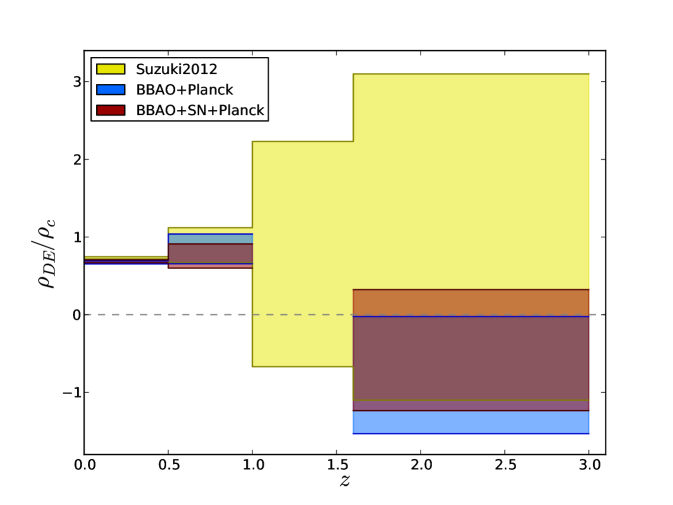
To conclude this section, we examine a model in which dark energy is characterized by specifying its energy density in four discrete bins of redshift: , , , and . This step-wise model is a useful complement to models that specify through parameterized descriptions of . The bins are chosen to be the same as the ones considered in a similar analysis by Suzuki2012 (their Table 8), who combined Union 2.1 SN data, WMAP7 CMB data (2011ApJS..192…18K, ), BAO from the combined analysis of SDSS DR7 and 2dFGRS (2002MNRAS.337.1068P, ), and the distance-ladder measurement of Riess11 . We fit simultaneously for in each of these bins and for the values of , , and , assuming to match Suzuki2012 . Within an individual bin, is held constant and evolves according to the Friedmann equation, but there are discontinuities in at bin boundaries to accommodate the discontinuous changes in . The matter density evolves as , where and denote values as usual.
Constraints on this model from our BAO+Planck and BAO+SN+Planck data combinations appear in Figure 11 and Table 5. As in our other models that allow time-varying dark energy, BAO and SN data both contribute significantly to the parameter constraints. Our results show a clear detection of non-zero dark energy density in each of the first two redshift bins at , and they are consistent with a constant energy density across this redshift range. Compared to Suzuki2012 , we obtain a significantly tighter constraint in the bin, where the CMASS BAO measurement makes an important difference, but a slightly looser constraint in the bin, where we do not incorporate a direct measurement. We obtain much poorer constraints in the bin because the JLA sample contains only 8 SNe with compared to 29 for the Union 2.1 sample. At our constraint is stronger thanks to the LyaF BAO measurement, but the uncertainty is large nonetheless, and the low LyaF value of leads to a preference for negative dark energy density in this bin, although consistent with zero at .
VI Alternative Models
We now turn to models with more unusual histories of the dark energy, matter, or radiation components. In part we want to know what constraints our combined data can place on interesting physical quantities, such as neutrino masses, extra relativistic species, dark energy that is dynamically significant at early times, or dark matter that decays into radiation over the history of the universe. We also want to see whether any of these alternative models can resolve the tension with the LyaF measurements at , which persists in all of the models considered in Section V. We begin with the early dark energy model, because understanding the origin of the constraints on this model informs the discussion of subsequent models.
VI.1 Early Dark Energy
In typical dark energy models, including all of those discussed in Section V, dark energy is dynamically negligible at high redshifts because its energy density grows with redshift much more slowly than . However, some scalar field potentials yield a dark energy density that tracks the energy density of the dominant species during the radiation and matter dominated eras, then asymptotes towards a cosmological constant at late times Albrecht00 ; Hebecker01 . These models ameliorate, to some degree, the “coincidence problem” of constant- models because the ratio of dark energy density to total energy density varies over a much smaller range.
As a generic parameterized form of such early dark energy models, we adopt the formulation of Doran & Robbers Doran06 , in which the density parameter of the dark energy component evolves with as
| (25) |
where and denote values as usual and is the dark energy density parameter at early times. A flat universe is assumed, with . The quantity is the effective value of the equation-of-state parameter today. At high redshift (), the denominator of the first term is , and approaches the constant value . This in turn requires a dark energy density that scales as in the matter-dominated era and as in the radiation-dominated era, though it is rather than that is specified explicitly. For , the model approaches CDM as goes to zero. There are other generic forms of models with early dark energy, as well as non-parametric descriptions (see discussion by Samsing12 ).

If dark energy is important in the pre-recombination era, then the boosted energy density in this era reduces the sound horizon by a factor relative to a conventional model with the same parameters Doran06 ; Samsing12 . Pre-recombination dark energy also influences the detailed shape of the CMB anisotropy spectrum by altering the early integrated Sachs-Wolfe contribution and the CMB damping tail Hojjati13 . Our analysis here incorporates the rescaling of the sound horizon, but we continue to use the compressed CMB description of Section II.3 and therefore ignore the more detailed changes to the power spectrum shape. Because of the exquisite precision of CMB measurements, the power spectrum shape may impose tighter constraints on early dark energy than the expansion history measurements employed here (see, e.g., Hojjati13 ). However, those constraints are more dependent on the specifics of the models being examined, both the dark energy evolution and other parameters that describe the inflationary spectrum, tensor fluctuations, relativistic energy density, and reionization.
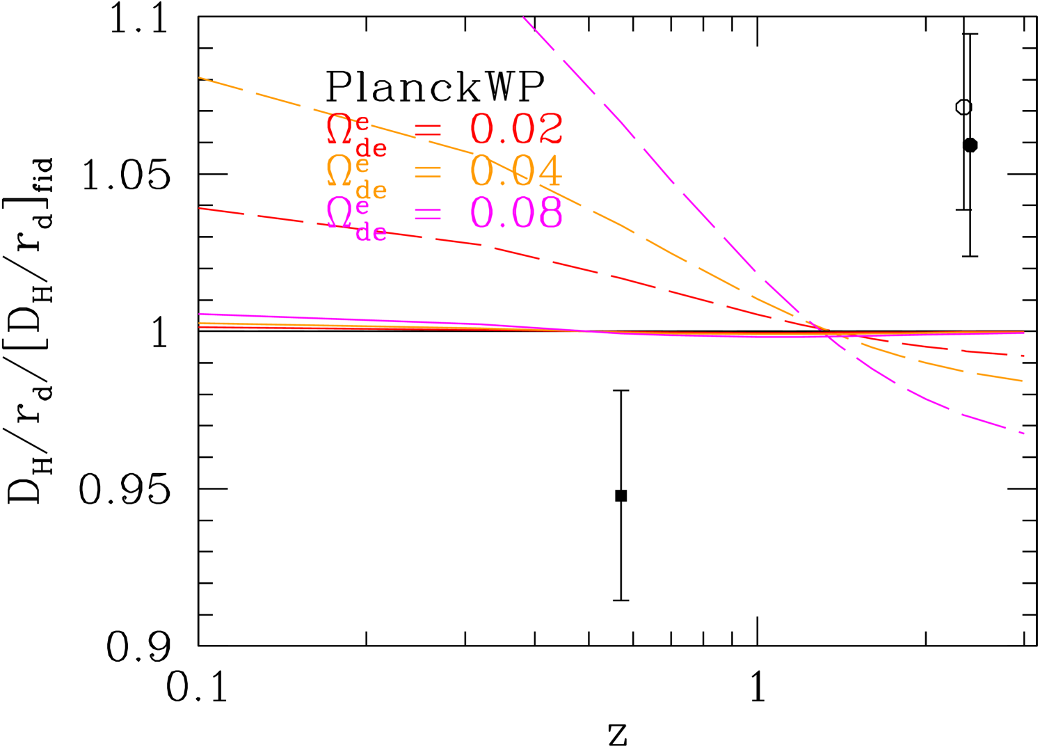
Figure 12 plots the evolution of and for models with 0.02, 0.04, and 0.08. We always adopt , but we constrain , , and by fixing , , and to the values in the best-fit Planck+WP CDM model, in effect forcing the errors in our compressed CMB description to zero. Solid curves incorporate the expected reduction of . Dotted curves show the case in which we instead keep fixed at its fiducial value of 147.49 Mpc. The latter case would be physically relevant in a model where dark energy is dynamically negligible in the pre-recombination era but approaches the evolution of equation (25) later in the matter dominated era. To highlight model differences, we scale all values to those of the fiducial CDM model, which corresponds to .
Remarkably, for the rescaled case, the predicted values of and change by less than 0.5% at all redshifts, even for . We can understand this insensitivity by considering the low and high-redshift limits for the simplified case of a flat cosmology with only matter and dark energy. The matter density at redshift is
| (26) |
where denotes the value as usual and we have used but relocated to the second factor. Using implies
| (27) |
For a cosmological constant, , so the ratio tends rapidly to zero at high redshift, but for the early dark energy model this ratio asymptotes instead to . Thus, at fixed , is higher in the early dark energy model by a factor , and is smaller by the same factor. This reduction in exactly compensates the rescaling of , leaving independent of .
At low redshift, conversely,
| (28) |
depends mainly on , since the evolution of is insensitive to moderate changes in and for . Therefore, to keep the value of fixed to the CMB constraint, one must increase by approximately so that both the low and high-redshift contributions to shrink by the factor required to compensate the change in . This change again forces to nearly the same value as the fiducial model with .
These scaling arguments are not perfect because they break down at intermediate redshifts and because a change in at fixed implies a change in , which itself affects the low-redshift evolution of . Nonetheless, the full calculation in Figure 12 demonstrates that for as large as 0.08 there is minimal change in at any redshift, and minimal change in in turn implies minimal change in . However, the values of are larger, and correspondingly smaller, for the successively higher curves in Figure 12. The combination is nearly constant, decreasing by just 0.14%, 0.24%, and 0.49% for , 0.04, and 0.08, respectively.
Reversing these arguments explains why and change rapidly with if stays fixed instead of rescaling (dashed curves in Fig. 12). In this case, must stay fixed to keep the angular scale of the acoustic peaks unchanged, so the decrease of high-redshift contributions to by requires a compensating increase of at low redshift. This requires a large fractional reduction in , since most of the contribution to comes from high redshift (e.g., 75% from ). This in turn leads to large deviations in and at low redshift. At high redshift, is again smaller by , but this now leads to a deviation in because it is no longer compensated by a smaller . Even for , fixing CMB observables requires a 4.3% reduction in . Furthermore, adding early dark energy in this case moves model predictions further from the CMASS and LyaF measurements of and further from the LyaF . We therefore expect tight constraints on in the case of fixed .
Figure 13 presents constraints on these early dark energy models from our MCMC analysis, with fixed to . We now account for uncertainties in the CMB constraints, using the compressed description of Section II.3. Note that we assume that the CMB constraints on and are not altered by the introduction of early dark energy, which might not hold in a complete analysis that uses the full CMB spectrum. The non-rescaled case is tightly constrained as expected, with a upper limit . SNe do not significantly improve these constraints, although they would play a larger role if we allowed as a free parameter. To summarize, adding early dark energy with fixed worsens agreement with our BAO measurements, and a dynamically significant value of is ruled out.
For rescaled , which is the physically expected case if remains constant back into the radiation-dominated era, we instead find a valley of near-perfect degeneracy between and . For and fixed , the expected degeneracy line is , marked by the red solid line in Figure 13. This prediction describes our numerical MCMC results extremely well. Along this line, there are models with relative to the best-fit CDM () model, at least out to . Including SNe again makes minimal difference to our constraints because the models along the degeneracy line predict nearly identical .
Although these models are degenerate with respect to our geometrical constraints, they predict different values of and different measures of structure growth. Intriguingly, non-zero with rescaled reduces tension with distance-ladder measurements of and with the level of matter clustering inferred from cluster masses, weak lensing, and redshift-space distortions. We discuss the impact on structure growth measures in Section VII.
As already emphasized, the detailed shape of the CMB power spectrum may impose much tighter constraints on early dark energy; e.g., for the specific case of the Doran-Robbers model, Hojjati13 infer at 95% confidence. However, the degeneracies identified here in the expansion history constraints are striking, and highlight the potential value of early dark energy studies that fully explore degeneracies with other parameters that affect the CMB power spectrum shape.
VI.2 Decaying Dark Matter

If dark matter is a metastable particle that decays into undetected radiation on a timescale comparable to , where the undetected radiation could be neutrinos or some other low-mass particle that interacts weakly enough to avoid detection (note that decay of a significant fraction of the dark matter into photons would need to have a very small branching ratio to be consistent with upper limits on cosmic backgrounds), then the matter density will decrease faster at low redshift than simple dilution (for an early discussion, see Turner1985 ). While the radiation density is boosted by dark matter decay, it subsequently decreases as , so the total energy density at low redshift is lower in a decaying dark matter (DDM) model than it would be for stable dark matter with the same high-redshift density. We initially considered this model as a potential explanation of the low inferred from the LyaF BAO. The heights of the acoustic peaks constrain the value of at the recombination epoch, but the reduced matter density at low redshift implies a lower value of The sound horizon scale is unchanged because the pre-recombination densities are unchanged. However, the full impact of introducing DDM is complex, because the values of and must change to keep at its precisely measured value, and because these changes and the dark matter decay itself affect the galaxy BAO observables and the LyaF value of .
We assume exponential decay of the dark matter (i.e., a constant decay rate), so that the governing equations for the decaying matter density (marked with subscript ) and decay products’ radiation density (marked with subscript ) are:
| (29) | |||||
| (30) |
The decay rate is dimensionless, and is the decay time in units of . However, we allow for the possibility that there are two kinds of dark matter, only one of which is susceptible to decay, so we introduce an additional parameter that is the ratio of this decaying component to the total dark matter density in the infinite past.666The earlier arXiv version of this paper had defined as a fraction of total matter density today. The other components of the model remain the same as those used for CDM. Initial conditions are chosen so that there is no energy density in the decay product radiation in the infinite past. We discuss some details of our solution technique in Appendix B.
An important subtlety in this analysis is that that the CMB peaks constrain the dark-matter density at the time of recombination, and hence the and densities that we feed into the compressed CMB likelihood corresponds to the densities the system would have had if the decay did not take place. Of course, the distance to the last scattering surface is still affected by the changes in the expansion history due to decaying dark matter.
Figure 14 shows two-dimensional posterior probability distributions in the plane for several values of . Although the data prefer no decaying dark matter, we see strong degeneracies that extend to surprisingly large values of . For , decay of nearly 50% of the primordial dark matter is allowed at 95% confidence. As expected, is negatively correlated with : the CMB constrains in the early universe, and if more dark matter decays then today is lower. There is also a weak correlation with the Hubble parameter (not shown), with rising by for .
To gain some understanding of this degeneracy, one can calculate the effective of the fluid composed of the combined decaying dark matter and the resulting radiation. At , and (the edge of our 68% contour), the effective takes values at , falling to at and at . With no decay, this component (which starts at the same energy density, as fixed by the CMB) would evolve with . The surprisingly small corrections to the total make it hard to constrain the decaying dark matter from expansion history data alone.
Using combinations of CMB, SN, and large-scale structure data sets, 2009JCAP…06..005D obtained a limit Gyr for the dark matter decay constant, using methodology similar to that described here but also including constraints from the full shape of the CMB power spectrum and the amplitude of matter clustering. A more recent analysis by 2014arXiv1407.2418A , using the Planck+WP CMB power spectrum and BAO measurements from BOSS and WiggleZ, obtained a somewhat stronger limit of Gyr. For a Hubble parameter , our limit for corresponds Gyr at 95% confidence level. A more detailed analysis by Blackadder2014 calculates the velocity distributions of daughter particles for varying assumptions about the decay products. For a daughter relativistic fraction of 1% and higher, they find Gyr based on analysis of Union 2.1 SNIa data in the context of CMB determined cosmological model. From these results we conclude that, somewhat surprisingly, the expansion history alone is not sufficient to significantly constrain the decay of dark matter into an unknown relativistic component.
We note that 2008PhRvD..77j3511G state a limit Gyr based on only the CMB acoustic scale and SNIa data available in 2008. We do not understand how these more limited data could lead to a stronger bound on the decay time, which suggests that the analysis of 2008PhRvD..77j3511G contains a hidden assumption.
VI.3 Massive Neutrinos
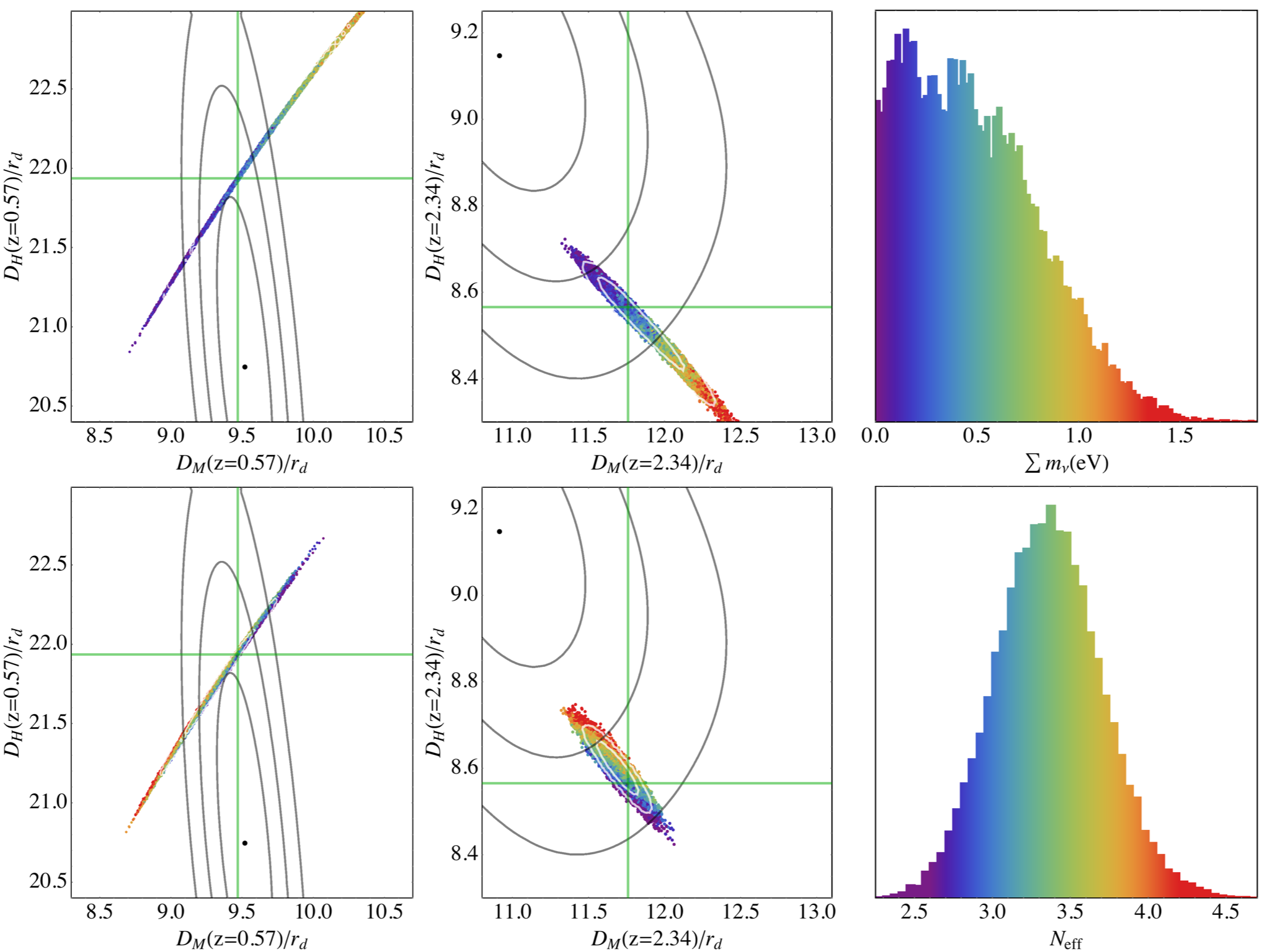

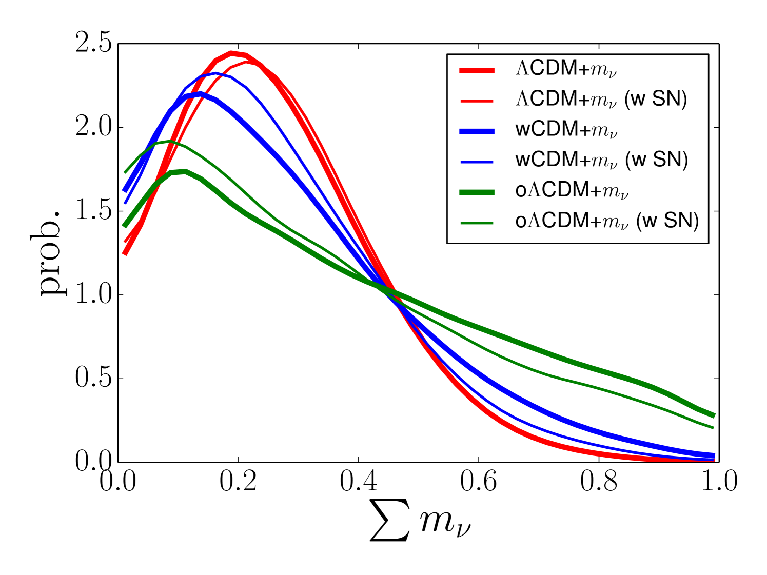
In addition to constraining dark energy and space curvature, measuring neutrino masses is a key objective of precision cosmology. Given CMB constraints that , the fractional contribution of neutrinos to the low-redshift matter density is , so neutrino masses have a noticeable cosmological impact if they are a significant fraction of an eV. Atmospheric and laboratory measurements constrain the mass splittings among the three standard-model neutrino species to be eV2 and eV2 Fogli:2012ua . This sets the minimum neutrino mass in a normal hierarchy, where , to , which motivates our assumption that in the standard CDM model. In the case of an inverted hierarchy, where , the sum of the neutrino masses must exceed , and for the degenerate neutrino mass case where , the minimum mass sum is approximately . These masses are well within reach of the cosmological experiments in the coming decade.
Neutrinos affect the CMB and large-scale structure differently from cold dark matter because they are still relativistic at the epoch of matter-radiation equality, because their linear clustering is suppressed on scales below Lesgourgues2006 , and because their high thermal velocities prevent them from clustering in small potential wells even in the non-linear regime LoVerde2014 ; LoVerde2014b . The relative suppression in the linear matter power spectrum is linear in the fraction density in neutrinos and is about (at best fit values of and ).
Measurements of matter clustering can constrain by detecting the suppression of small scale power. Expansion history measurements, which we focus on here, can constrain because of their transition from a relativistic species whose energy density scales as to a non-relativistic species whose energy density scales as , effectively the converse of decaying dark matter. Specifically, the CMB acoustic peaks constrain almost independently of , but the matter density that affects late-time expansion rates and distances is . With other parameters held fixed, a neutrino mass-sum increases the late-time matter density by 1.4%, which is significant given the extremely precise CMB measurement of and precise distance scale measurements from BAO. In practice, changing leads to adjustments in other parameters to seek a global best fit. Although the neutrino mass influences the sound horizon (eq. 16), this impact is small for the range of allowed by our constraints ( for ).
The top row of Figure 15 compares the CMASS and LyaF BAO constraints to the predictions of CMB-constrained, flat CDM models with as a free parameter, in the same format as Figure 7. The Planck CMB chain used here is base_mnu_planck_lowl_lowLike_highL_Alens, where we have selected a chain that marginalizes over the lensing amplitude parameter for reasons discussed below. The base Planck CDM model adopts , but this chain allows down to zero. While is allowed by the CMB data alone, this mass significantly worsens agreement with the BAO data, both at and at . Higher increases and thus decreases , moving further from the LyaF measurement. Additionally, because of the tight CMB constraint on , the reduction in at high redshift must be compensated by changes in and that raise at low redshift, so , , and all increase, again moving away from the BAO measurements. Conversely, moving towards slightly improves agreement with the LyaF BAO because increases while , which has a large contribution from lower redshifts, decreases. However, the same change worsens agreement with the CMASS BAO, which are already well fit by the base model with .
The red curve in the upper panel of Figure 16 shows the purely geometric constraint that arises from combining just the compressed CMB description with galaxy and LyaF BAO data. This constraint is surprisingly tight at (at 95% c.l.), and it is independent of mass constraints based on the suppression of structure growth by neutrino free-streaming. Adding SN data does not significantly improve this constraint. The geometrical constraint on neutrino mass weakens if we allow either curvature or , as shown by the blue and green curves in the lower panel of Figure 16. Because neutrinos influence the observables only via the effect of on distances and expansion rates, adding another degree of freedom introduces degeneracy. In these cases, including SN data does improve the neutrino mass constraint, as shown by the thin curves. The improvement is not dramatic, indicating that our multiple BAO measurements can break the degeneracy themselves to a significant degree.
The 95% upper limits on for the various models and data combinations we have considered are listed in Table 6. Direct measurements of matter clustering at low redshift can be a powerful diagnostic of neutrino masses because they are sensitive to the distinctive effect of suppressing small scale power, which is not easily mimicked by other parameter variations. We return to this point in Section VII.
In the top panel of Figure 16, the green curve shows the result of full fitting using the cosmomc machinery. The constraint tightens significantly to eV (at 95% c.l.). This number is the same as the Planck collaboration constraint for Planck+BAO PlanckXVI , even though we use more and better constraining BAO data. This exercise demonstrates that the compression into , , and is missing important information that the CMB provides on neutrino mass. The extra information is in the constraint on the amplitude of low-redshift matter clustering that comes from the smoothing of the acoustic peaks in the CMB power spectrum by weak gravitational lensing. The BAO information in this case fixes the matter density of the universe, thus allowing inference on the amplitude of matter fluctuations and hence neutrino mass to be determined from the smoothness of the peaks (the CMB only constraint is eV (PlanckXVI, )). The role of CMB lensing is further demonstrated by the blue curve in the top panel. Here we have run a cosmomc chain that, in addition to having as a free parameter, marginalizes over a parameter that multiplies the predicted lensing signal, effectively removing the lensing information. (The base model fixes .) The result here is very similar to that found by using the compressed CMB description.
For CDM, fitting the CMB temperature power spectrum from Planck (together with WMAP polarization and high- data from ground-based experiments) yields (PlanckXVI, ), showing that the lensing signal measured in the Planck power spectrum is significantly stronger than the predicted signal based on extrapolating the observed CMB fluctuations forward in time. A larger neutrino mass suppresses the low-redshift clustering, exacerbating this tension, which is why the limit is considerably tighter when is fixed to unity. However, the Planck measurement of lensing through the CMB 4-point function does agree with (PlanckXVI, ). These internal tensions on the lensing signal within the CMB data alone suggest that one should be cautious in using them to constrain . The red curve is thus a more conservative inference, using only geometric constraints plus the CMB constraints on and . It is impressive that even a 3.5% contribution of neutrinos to () is enough to be substantially disfavored by these expansion history measurements.
| Combination | Model | 95% limit on |
|---|---|---|
| BAO+Planck(full) | CDM | 0.25eV |
| BAO+Planck(full) | CDM + free | 0.43eV |
| BAO+Planck | CDM | 0.56eV |
| BAO+Planck | CDM | 0.68eV |
| BAO+Planck | CDM | 0.87eV |
| BAO+SN+Planck | CDM | 0.56eV |
| BAO+SN+Planck | CDM | 0.61eV |
| BAO+SN+Planck | CDM | 0.84eV |
VI.4 Extra Relativistic Species
If the universe contains extra relativistic degrees of freedom beyond those in the standard model, these increase the expansion rate during the radiation dominated era and shift the epoch of matter-radiation equality, thereby altering the sound horizon, the shape of the matter power spectrum, and the history of recombination. Extra radiation is usually parameterized by the quantity , where corresponds to the amount of radiation that an extra massless thermalized neutrino species (i.e., a fermion that thermally decouples before electron-positrion annihilation) would produce. In general, however, there is no requirement that be an integer. The standard model has and .

The bottom row of Figure 15 shows the probability distribution for from CMB data alone (right panel, from the chain base_nnu_planck_lowl_lowLike_highL). which peaks at , with a 95% confidence range . The middle panel shows that values of at the upper end of this range can noticeably improve consistency with the LyaF BAO measurement, pushing the predicted values of up and down so that they lie within the 95% likelihood contour of the BAO data. However, high values of reduce the predicted values of and at , worsening agreement with the galaxy BAO measurements.
We can understand these trends by arguments similar to those given for early dark energy in Section VI.1. An increase of reduces the sound horizon by 3.2% (eq. 17) because of the higher expansion rate in the early universe. Maintaining the precisely measured value of requires changes in and to reduce by the same factor. Some of this reduction can be accomplished by raising , and thus raising at high redshift, but is already tightly constrained by the heights of the acoustic peaks. Therefore, the fractional change to is much lower than the fractional change to , and the value of rises. To maintain , the value of (which controls the low-redshift contribution to the integral) must increase by more than the drop in . Because is an integral over all , the ratio drops even as rises. At , where the value of retains sensitivity to , both and drop as increases.
A change in has multiple effects on the CMB, which renders our compression into a 3-variable matrix questionable. For this section of the paper, therefore, we have run cosmomc chains using the full Planck+WP CMB information, while still treating the BAO data as measurements of and . We have checked that using our simplemc chains, which adopt the compressed CMB description, yields qualitatively similar but quantitatively different results. We assume a flat universe with a cosmological constant, but we treat the tensor-to-scalar ratio as a free parameter and marginalize over it, since there is no theoretical reason to expect . While allowing free would not alter the compressed CMB constraints used elsewhere in the paper, it has an impact here because and have partially degenerate effects on the shape of the CMB power spectrum.
Red contours in Figure 17 show confidence intervals in the plane obtained by combining the CMB data with LyaF BAO alone. The allowed range of is larger here than in Figure 15 because we do not fix . As one would expect from Figure 15, the addition of LyaF BAO pulls the preferred value of upward, with a best-fit value of and significantly disfavored. However, the galaxy BAO measurements prefer and have higher precision, so when they are added (green contours) the allowed range shifts downward to (68%) or (95%). Higher correlates with higher for the reasons discussed above, and with and as an additional degree of freedom our BAO+CMB constraint is . Adding SN data does not significantly shift these contours once galaxy BAO are included. As shown in Figure 10, introducing as a parameter reduces by 0.75 relative to CDM, with nearly all of the change coming from a slightly better fit to the LyaF BAO data.
One complication in constraining models is that changing the radiation density can alter the broadband power spectrum shape enough to affect the BAO fitting procedure itself. Anderson14 find that the compression of BAO data into the plane (in other words, the fact that the inferred values of and are independent of the adopted fiducial model) breaks down in the presence of extra radiation at a % level. This effect is negligible compared to the statistical errors in the LyaF BAO data, but it is not completely negligible relative to the galaxy BAO errors. A more exact treatment of the constraints therefore requires refitting the BAO data themselves, but we would expect only small shifts relative to the constraints reported here. We plan to revisit this question when the final BOSS measurements are available.
VI.5 A Tuned Oscillation

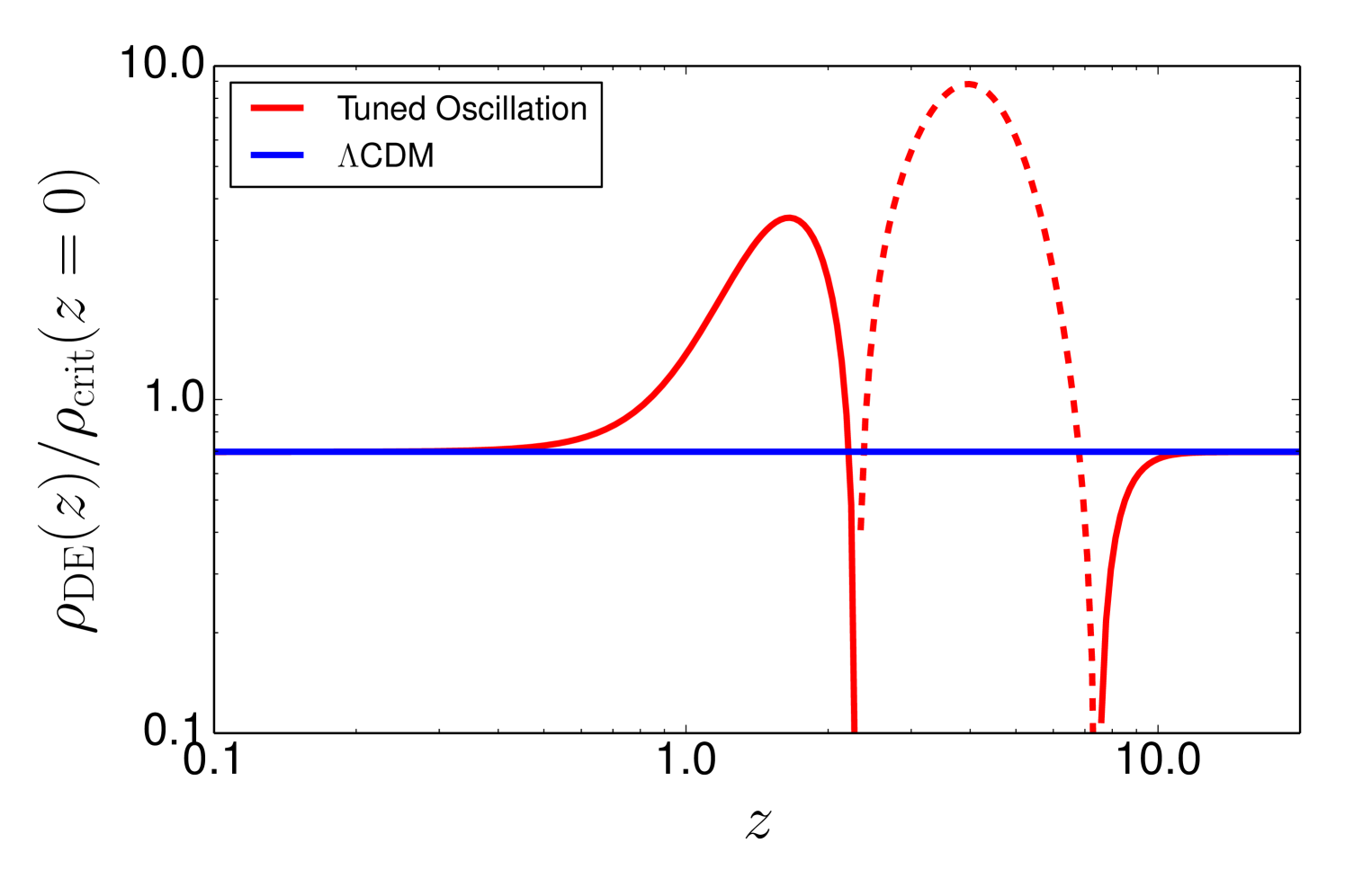
While the model moderately reduces tension with the LyaF BAO data, none of the models we have considered produces a truly good fit to all the measurements. To understand what is required to achieve a good fit, we have constructed an artificial model that maintains the mathematical link between and but has the freedom needed to fit all the BAO and CMB data at the level. We consider a flat universe whose angular diameter distance is given by
| (31) |
where denotes a Gaussian in with mean and variance and is an amplitude parameter. It is clear that such model can, for a sufficiently localized Gaussian perturbation, fit the low-redshift and CMB data with sufficient goodness of fit. Given three parameters it has enough flexibility to also match our points. Figure 18 plots the best fitting model of this form. The Hubble parameter undergoes an oscillation between and , which allows it to match the LyaF and CMASS values of and to change at without altering the low and high redshift values.
This model reduces the overall by 6.6 with three extra degrees of freedom, a considerable improvement over any other model we have investigated (see Figure 10). Generically, any small perturbation to the Friedmann equation that is able to improve fits to our LyaF data runs afoul of CMB and/or galaxy BAO constraints. This model works because it is fine-tuned to change distances near but not upset the distance to the last-scattering surface. However, the model is physically extreme, as demonstrated in Figure 19, where we have converted into an implied dark energy density via the Friedmann equation. Producing the desired oscillation in requires a negative between and (see eq. 27). Sahni2014 argue that the BOSS LyaF measurements may be explained in a modified gravity model that alters the Friedmann equation itself in a physically motivated way, but more work is needed to determine whether any such model can provide a good fit to all of the BAO measurements while satisfying CMB constraints.
The difficulty in finding a well motivated model that matches the BOSS LyaF measurements suggests that the tension with these measurements may be a statistical fluke, or a consequence of an unrecognized systematic that either biases the central values of and or causes their error bars to be underestimated. Analyses of the final BOSS data set will address both of the latter points, as they will allow more exhaustive investigation of analysis procedures and tests against larger suites of mock catalogs. Addressing the first point will require high-redshift BAO measurements from new data sets, such as the Ly emission-line galaxy survey of HETDEX Hill2004 or a much larger LyaF sample from DESI Levi2013 .
VII Comparison to Structure Growth Constraints
The Planck cosmology papers highlighted a tension between the predictions of the CMB-normalized CDM model and observational constraints on matter clustering at low redshifts, from cluster abundances, weak gravitational lensing, or redshift-space distortions. We now revisit this issue with our updated BAO and SN constraints and our broader set of models, to see whether these tensions persist and whether they are significantly reduced in some classes of models.
Low-redshift measurements of cluster abundances and weak lensing most tightly constrain the parameter combination with (see discussions in Weinberg13 and references therein). As representative but not exhaustive examples of constraints at we adopt: from tomographic cosmic shear measurements in the CFHTLens survey Heymans13 ; from cosmic shear measurements in the Deep Lens Survey777The authors do not quote their results in this form, so this constraint has been eyeballed from their Fig. 25 Jee13 ; from the combination of galaxy-galaxy lensing and galaxy clustering in the SDSS Mandelbaum13 ; from the mass function of X-ray clusters observed with Chandra and ROSAT Vikhlinin09 ; from stacked weak lensing of clusters in the SDSS Rozo10 ; and from Sunyaev-Zeldovich clusters in Planck, where we have taken the value quoted for a 20% X-ray mass bias PlanckXX . These estimates are shown as red points with error bars in Figure 20a, where we have scaled the amplitudes to using the formulas listed above and retained the original fractional errors. We compare to model predictions of , treating 0.4 as a representative slope for these constraints.
Recently 2014arXiv1408.4742M have completed an independent analysis of tomographic cosmic shear in the CFHTLens data and confirmed the findings of Heymans13 . Conversely, 2014arXiv1407.4516M have performed a cluster mass function analysis using extensive weak lensing calibration of X-ray cluster masses and found , which corresponds to higher for than the other cluster studies listed above. We also show this point in Figure 20a, with the caution that the scaling with reported by 2014arXiv1407.4516M is quite different from that of the other analyses.
For redshift-space distortion (RSD), the point labeled Beu14 in Figure 20b shows the recent BOSS CMASS measurement by Beutler14 , which yields at , where is the linear fluctuation growth rate. This analysis fits simultaneously for redshift-space distortion and the Alcock-Paczynski (AP) effect Alcock79 . Here we have used the error for fixed value of the AP parameter because the geometry is well constrained by our BAO+SN+CMB data, so that the fractional error in the AP parameter is much smaller than the 6.4% error on . The point labeled Sam14 shows the estimate from the same data set using a power spectrum analysis instead of a correlation function analysis. Since the data are the same, the difference from Beu14 provides an indication of the uncertainties associated with modeling systematics. Other analyses of redshift-space clustering in BOSS 2013MNRAS.433.3559C ; 2013MNRAS.433.1202S and the WiggleZ survey 2011MNRAS.415.2876B yield compatible results. We also plot an estimate of from an analysis of smaller scale redshift-space distortions in the CMASS sample by Reid14 , which adopts more aggressive modeling assumptions and achieves a substantially smaller statistical error.
At higher redshift, the 1-dimensional flux power spectrum of the Lyman- forest probes the underlying matter clustering, with the tightest constraints on comoving scales of a few Mpc Croft02 ; McDonald05 ; Palanque13 . Here we take the result from the BOSS analysis of Palanque13 , who find when fitting a CDM model to the 1-d at redshifts . We translate this result to a constraint on by using the growth factor at for their central value of . This measurement is indicated by a point with error bar in Figure 20c.
Given the wide range of models that we wish to consider and the several-percent errors on the observational data, we have opted for an approximate method of computing clustering amplitude predictions that is accurate at the 0.5-percent level or better. Following the strategy of Hu04 and Weinberg13 , we first use CAMB calculations to calibrate a Taylor expansion for the value of about a fiducial Planck CDM model, finding
| (32) |
Here is the amplitude of primordial curvature perturbations at the scale Mpc-1. This formula updates equations (46)-(47) of Weinberg13 , which were expanded about a WMAP7 fiducial model. The fairly strong -dependence arises because of the conversion from a power spectrum predicted in Mpc units based on cosmological parameter values to an amplitude defined on a scale of . We have made numerous checks of this formula against full CAMB calculations for models in the parameter ranges allowed by Planck + WP data, finding accuracy of better than 0.1% for CDM, for CDM with , and for CDM with , and accuracy better than 0.5% for models with . While equation (32) correctly reflects the response of to an isolated change in , in practice the CMB-preferred values of , , , , and all increase when increases, with the result that higher models end up predicting higher clustering amplitudes. We have not attempted to incorporate the effects of non-zero neutrino mass in this formula because the suppression of clustering by neutrino free streaming is redshift and scale dependent (see Rossi14 for useful representations).
Except in early dark energy models, the value of is essentially independent of dark energy parameters because dark energy is dynamically insignificant at (e.g., for a cosmological constant). To evolve forward to , 0.57, or 0, we use the approximate integral formulation of the growth factor from equation (16) of Weinberg13 , which simply integrates the growth rate approximation of Linder05 , with . Spot checks against exact calculations with cosmomc indicate that this approach is accurate to 0.3% or better for models with and other parameters in the range allowed by our CMB+BAO+SN data, although it becomes less accurate for more extreme parameter values (especially of ). For , CAMB yields a ratio that is 0.5% lower than for , with little dependence on other parameters, so we also multiply all of our low-redshift values by 0.995 to account for this effect.
We determine the mean values and error bars on the predicted growth observables for our models by computing the posterior-weighted mean and dispersion of , , or for the parameter values in our MC chains, using the above approximations for . Because our chains do not actually use or include values of , we compute for the fiducial value in equation (32) and add a fractional error (based on the Planck+WP column in Table 5 of PlanckXVI ) of 1.25% in quadrature to the MCMC error to account for the 2.5% error in , which is proportional to . Inspection of Planck chains indicates only weak correlations between and other cosmological parameters, so the approximation of an independent error contribution added in quadrature should be adequate. We also add in quadrature a fractional error of 0.3% to represent potential errors of our approximate growth calculations, though our spot checks indicate higher accuracy than this.
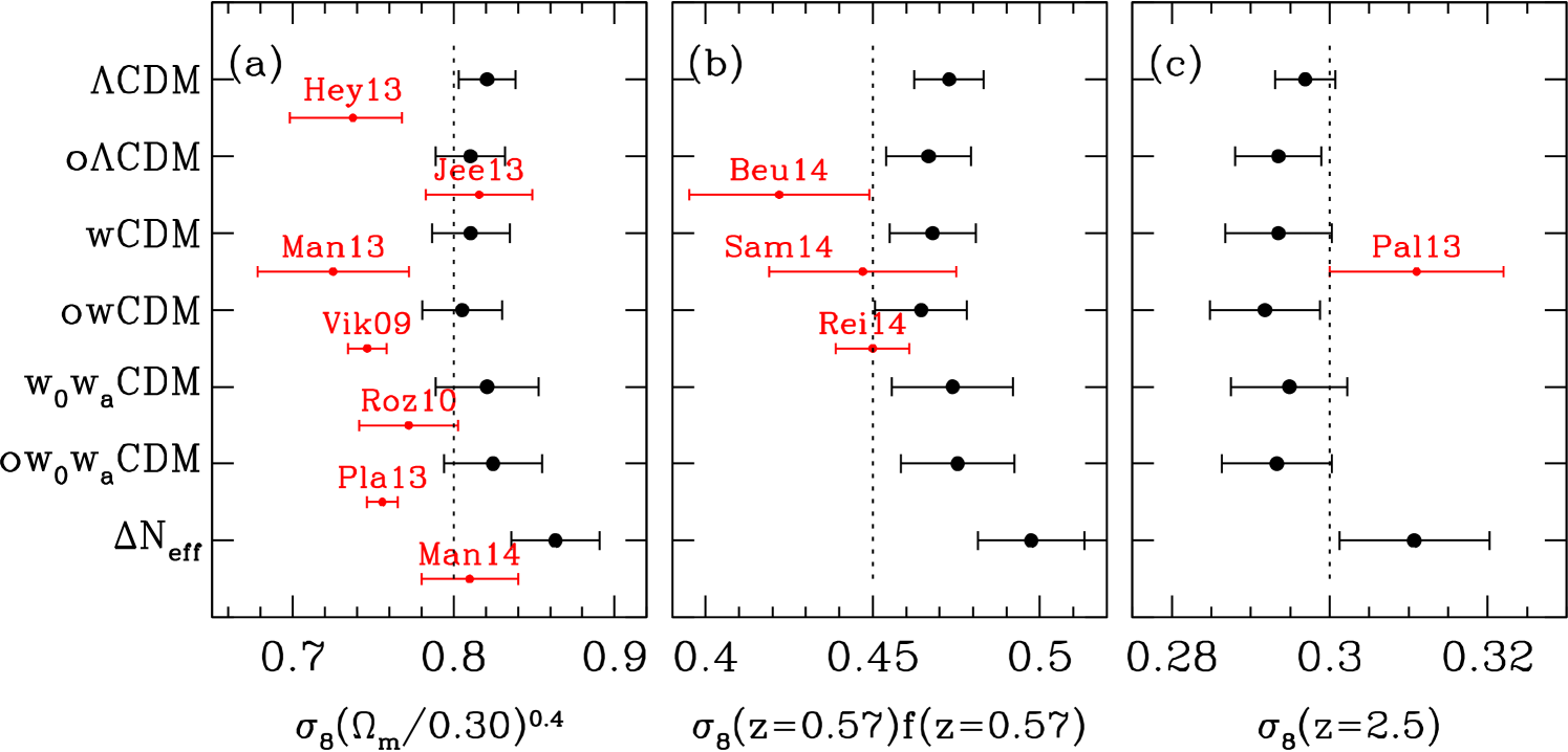
Figure 20a shows a persistent offset between the predicted amplitude of matter clustering and the majority of observational estimates from weak lensing and cluster masses. For CDM, where the model predictions are best constrained, the statistical significance of the tension with any given data set is usually only or smaller. However, the sign of discrepancy is usually the same, so the overall significance is high unless multiple analyses are affected by a common systematic. The important exceptions are the cosmic shear measurement from the Deep Lens Survey Jee13 and the recent cluster analysis of 2014arXiv1407.4516M , which both agree well with the CDM prediction. The authors of 2014arXiv1407.4516M emphasize that theirs was a “blind” analysis in which technical choices about data cuts and procedures were made without knowing their eventual impact on inferred cosmological parameter values. Our predicted value of is somewhat lower than the value inferred by PlanckXVI from CMB data alone (Planck+WP+highL), in part because the BAO data pull towards lower , and in part because our compressed CMB description does not include the lensing information in the Planck power spectrum, which pulls towards higher . For more flexible dark energy models, central values of remain within the range found for CDM, and the error bars are moderately larger. The tension with the data is moderately reduced in these models, but not eliminated. A formal assessment of this reduced disagreement is difficult because the true level of systematic uncertainty in the low-redshift measurements is itself uncertain, but at a qualitative level this reduction appears too small to favor adopting one of these more complex models.
Figure 20b shows an offset of similar magnitude between the predictions of our standard dark energy models and the redshift-space distortion measurement of Beutler14 at . However, the statistical significance of this tension is low because of the statistical error on the measurement, and the power spectrum analysis of 2014MNRAS.439.3504S yields a higher central value. The more precise determination from Reid14 , which draws on simulation-based modeling of non-linear scales, overlaps the CDM prediction at . A recent analysis that combines galaxy clustering and galaxy-galaxy lensing of CMASS galaxies More14 yields constraints in the plane that are consistent with the CDM model predictions, but the current statistical errors are large enough to be compatible with the central values from any of the redshift-space distortion analyses shown here. In contrast to the lower redshift results, Figure 20c shows that the predicted clustering amplitude at in our standard models is lower than that inferred from the LyaF power spectrum, though consistent at .
In the model, where we assume a CDM cosmology but allow extra relativistic species, the preferred value of is higher than the standard value of 3.046, as shown previously in Figure 17. Because of the correlation of with other cosmological parameters in CMB fits, the central value of the clustering amplitude predictions shifts upwards, while the freedom in broadens the error bar relative to standard CDM. These changes noticeably increase the tension with the clustering measurements at and the RSD measurements at , though they improve agreement with the LyaF power spectrum at . Overall, current clustering measurements provide moderate evidence against extra relativistic species, though a firmer understanding of systematic uncertainties in these measurements will be needed to draw solid conclusions.
Massive neutrinos have a redshift- and scale-dependent impact on matter clustering, which changes between the linear and non-linear regimes. We have not attempted a full examination of free- models in this section because the summary of the observational results in terms of constraints may not adequately capture the effect of massive neutrinos on the clustering observables. A value of , near the 95% upper bound inferred from our compressed CMB description and BAO constraints, would lower the predicted value of in a Planck+WP-normalized CDM model by about 12% relative to . A value , near the upper bound that we find when combining the full Planck likelihood with BAO data, would produce a 6% suppression of . These numbers are somewhat different from what a naive expectation based on linear suppression would indicate because CMB degeneracies are important at these relatively large neutrino mass fractions. Even the lower value is enough to remove the tension seen in Figure 20a. However, the corresponding decrease in produces a significant discrepancy with the LyaF measurement in Figure 20c, and a full analysis that models the LyaF power spectrum based on hydrodynamic simulations with a massive neutrino component leads to a stringent upper limit on neutrino mass Palanque14 .
As discussed in Section VI.1, our geometric constraints are nearly degenerate with respect to the presence of an early dark energy component, provided this early dark energy is present in the radiation-dominated epoch as well as the matter-dominated epoch and therefore shrinks the scale of the sound horizon. Increasing the early dark energy fraction reduces the value of (see Fig. 13) and will also suppress growth of structure relative to CDM. Predictions of structure for early dark energy are subtle because of the combined impacts of CMB normalization, the imprint of early dark energy fluctuations on the CMB itself, and the post-recombination growth rate. We therefore defer detailed investigation of early dark energy models to future work and make the qualitative observation that an early dark energy component will go in the direction of reducing tensions with low redshift clustering measurements.
VIII Conclusions
In the decade since the first observational detection of baryon acoustic oscillations, BAO analysis has emerged as one of the sharpest tools of precision cosmology. Its power arises from the grounding of its absolute distance scale in straightforward underlying physics, from the distinctiveness of a feature that is localized in scale and thus not easily mimicked by observational systematics, and from its insensitivity to non-linear gravitational evolution and galaxy formation physics (a consequence of the large scale of BAO). The principal challenge of the method is that one must map enormous cosmic volumes to obtain good statistical precision. Building on the legacy of 2dFGRS, SDSS-I/II, 6dFGS, and WiggleZ, BOSS has made major progress on this challenge, with distance scale measurements of precision at , 0.57, and 2.34. The combination of BAO measurements with Planck+WP CMB data and the JLA SNIa compilation leads to numerous significant constraints on dark energy, space curvature, and the cosmic matter and radiation density.
If we treat BAO as an uncalibrated standard ruler, assuming only that it is constant in time, then the combination of galaxy and LyaF BAO measurements yields a strong () detection of dark energy, independent of any other cosmological data. If we assume that the angular acoustic scale of the CMB represents the same standard ruler, then the resulting constraints in an CDM model collapse around a flat universe dominated by dark energy, with , . Thus, high-precision measurements of a common standard ruler at , , and already lead to strong constraints on the cosmological model.
BAO become much more powerful when we incorporate the absolute calibration of the sound horizon using CMB measurements of the matter, baryon, and radiation energy density (eq. 16). With Planck+WP CMB data, residual uncertainties in and leave only 0.4% uncertainty in the acoustic scale Mpc assuming a standard radiation background with three neutrino species. One particularly interesting application of this calibration is to combine galaxy BAO measurements with the high-precision measurements of relative distances from Type Ia SNe to infer . The addition of the SN data makes the inferred value of insensitive to uncertainties in the dark energy model, which would otherwise affect the extrapolation of the distance scale from the moderate redshifts of the BAO measurements down to . With our standard BAO and SN data sets, this inverse distance ladder measurement yields , where the 1.7% uncertainty includes the Planck+WP uncertainty in . This value agrees perfectly with the value inferred from current CMB data under the much stronger assumption of a flat CDM model, an important consistency test of the standard cosmology. It is lower than most recent estimates using a Cepheid-based distance ladder. Our measurement of does rely on the assumption of a standard cosmic radiation background, and the directly constrained parameter combination is . A convincing discrepancy with conventional distance-ladder determinations of could not be resolved by appealing to the late-time behavior of dark energy. It would point instead to non-standard physics in the pre-recombination universe, such as extra relativistic degrees of freedom or early dark energy, which can shrink and thus raise the inferred value of .
The full combination of CMB, BAO, and SN data places strong constraints on dark energy and space curvature, as summarized in Figure 8 and Table 4. In models that allow both and non-zero curvature, the BAO and SN data are highly complementary. For the CDM model, we find and . For models with , the constraint on evolution remains poor, with in CDM, but the value of at the pivot redshift where it is best constrained remains close to . A striking feature of Table 4 is that as degrees of freedom are added to the cosmological model the best-fit values of parameters barely change, always remaining close to those of flat CDM.
These models are fit to a total of 43 observables: three in our compressed description of the CMB, 31 for the compressed SN data, five for the galaxy BAO data ( from 6dFGS, MGS and BOSS LOWZ, and from BOSS CMASS), and four for the LyaF BAO ( and from forest auto-correlation and from quasar-forest cross-correlation). The CDM model, with three free parameters (, , and the absolute magnitude normalization for SNIa), has for 40 d.o.f., which is statistically acceptable.888Note that Figure 10 omits the CMB data from the accounting, so it has three fewer d.o.f. The decrease in for the alternative models is not enough to justify the addition of parameters; for example, the addition of three free parameters in CDM reduces by only 1.33. However, the best-fit models in all of these cases are in significant tension with the LyaF measurements on their own, typically at the level. The LyaF data have little impact on the best-fit parameter values in any of these models, not because they agree well with the model predictions but because parameter changes that would significantly improve agreement with the LyaF run afoul of the higher precision galaxy BAO measurements. Moreover, because the LyaF measurements have lower but higher than expected in the best-fit CDM model, many parameter changes that would improve the fit to worsen the fit to , and vice versa.
We have examined several models with non-standard dark energy or dark matter histories or non-standard radiation backgrounds. Early dark energy that has constant in the radiation and matter dominated eras (before evolving towards a cosmological constant at low redshift) alters the sound horizon and evolution of and . Remarkably, the cancellation of these effects leaves the BAO observables and nearly unchanged (including at ), even for as large as 0.3, so that the observations incorporated in our fits still allow a substantial early dark energy component. Because of the smaller , such model fits yield a higher and lower , and the suppression of growth by early dark energy is likely to reduce the amplitude of low-redshift matter clustering. Full CMB power spectrum analyses yield stronger but more model-dependent constraints on early dark energy through its influence on the shape of the acoustic peaks and the structure of the damping tail Hojjati13 . Nonetheless, the ability of these models to match expansion history constraints while improving agreement with local and structure growth measurements suggests that they merit further investigation.
If “early” dark energy becomes important only after recombination, so that it does not alter the acoustic scale, then CMB+BAO data impose strong constraints, with at 95% confidence. A similar conclusion applies to other physical effects that distort the low-redshift distance scale relative to and the distance to last scattering. In particular, we considered models in which a component of dark matter decays into radiation on cosmological timescales, boosting and decreasing at low redshifts. The BAO+CMB data limit the fraction of dark matter that can decay by to below 3% (95% confidence).
With respect to expansion history, massive neutrinos are in some sense the converse of decaying dark matter: they are relativistic at the epoch of recombination, but at low redshift they increase the matter density relative to the value inferred from the CMB acoustic peaks. The purely geometric constraints that come from BAO and our compressed CMB description yield a 95% confidence upper limit of assuming CDM, with moderately weaker limits for models that allow or non-zero (see Table 6). If we use full Planck CMB chains in place of our compressed description we obtain the significantly stronger limit , a difference driven by the relatively high amplitude lensing signal detected in the Planck power spectrum. Measurements of low-redshift matter clustering can yield more sensitive limits on neutrino masses, and potentially a measurement of through its impact on structure growth, but the expansion history constraints are robust and impressively stringent on their own.
Adding relativistic degrees of freedom can noticeably improve the agreement with the LyaF BAO, and if we combine only CMB and LyaF data the preferred is . However, increasing worsens agreement with the galaxy BAO data, and when we consider our full data combination we find . Increasing reduces the value of and thereby leads to a higher inferred ; for a model with free and free tensor-to-scalar ratio we find a marginalized constraint . We caution that modifying the radiation background alters the shape of the acoustic peaks, an effect not accounted for in the BAO measurements used here; we expect this effect to be smaller than our statistical errors, but perhaps not negligible.
Among these alternative models, only the model with free can reduce the tension with the LyaF data, and even there the reduction is small once the galaxy BAO constraints are also imposed. We did construct a model with a tuned oscillation in that reproduces both the and measurements from the LyaF BAO while continuing to satisfy all other constraints. However, this model requires non-monotonic evolution of and thus of , which is difficult to achieve in any model with non-negative dark energy density. The artificiality and physical implausibility of this model, and the failure of our more physically motivated models, illustrate how difficult it is to obtain a good fit to the BOSS LyaF BAO measurements. This difficulty suggests that the tension of simpler models with the LyaF data is a statistical fluke, or perhaps reflects an unrecognized systematic in the BAO measurement, but it highlights the importance of further measurements of and at high redshifts.
The cosmological constraints considered here are essentially geometrical, tied to the expansion history of the homogeneous universe. As a further test, we have computed the predictions of our models for low redshift measurements of matter clustering. Confirming previous findings, but now with tighter cosmological parameter constraints, we find that a CDM model normalized to the observed amplitude of CMB anisotropies predicts cluster masses, weak lensing signals, and redshift-space distortions that are higher than most observational estimates. The tension with individual data sets is only , and the measurements themselves may be affected by systematics. However, the direction of the discrepancy is consistent across many analyses (though not all of them). The additional freedom in standard dark energy models does not reduce this tension because the parameter values allowed by our data are always close to those of CDM. Massive neutrinos can reduce the tension by suppressing structure growth on small scales (lowering ), an effect that is small but not negligible for neutrino masses in the range allowed by our fits. Conversely, increasing above the standard value of 3.046 leads to higher predicted values of because of correlation with other cosmological parameters, thus amplifying the tension. As previously noted, early dark energy may reduce the tension with the clustering data, both because it suppresses growth of structure during the matter dominated era and because the reduced value leads to higher and lower when combined with CMB constraints. Our standard CDM fits produce good agreement with the matter clustering amplitude inferred from the LyaF power spectrum at ; this agreement is itself an important constraint on neutrino masses or other physical mechanisms that reduce small scale clustering Palanque14 .
The application of the BAO technique to large cosmological surveys has enabled the first percent-level measurements of absolute distances beyond the Milky Way. In combination with CMB and SN data, these measurements yield impressively tight constraints on the cosmic expansion history and correspondingly stringent tests of dark energy theories. Over the next year, the strength of these tests will advance significantly with the final results from BOSS and with CMB polarization and improved temperature maps from Planck. In the longer term, BAO measurements will gain in precision and redshift range through a multitude of ongoing or planned spectroscopic surveys, including SDSS-IV eBOSS, HETDEX, SuMIRE, DESI, WEAVE, Euclid, and WFIRST.999See Weinberg13b for a brief summary of these projects and references to more detailed descriptions. These data sets also enable precise measurements of matter clustering through redshift-space distortion analyses, the shape of the 3-dimensional power spectrum, and other clustering statistics. In combination with the expansion history constraints, these measurements can test modified gravity explanations of cosmic acceleration and probe the physics of inflation, the masses of neutrinos, and the properties of dark matter. In parallel with these large spectroscopic surveys, supernova measurements of expansion history are gaining in precision, data quality, and redshift range, and weak lensing constraints on matter clustering are advancing to the percent and sub-percent level as imaging surveys grow from millions of galaxy shape measurements to hundreds of millions, and eventually to billions. From the mid-1990s through the early 21st century, improving cosmological data sets transformed our picture of the universe. The next decade — of time and of precision — could bring equally surprising changes to our understanding of the cosmos.
Acknowledgements
We thank Eric Linder for useful discussions of early dark energy and structure growth. We also thank Savvas Koushiappas and Gordon Blackadder for alerting us to an error in the decaying dark matter section of the preprint version of this paper and answering our questions as we corrected it.
Funding for SDSS-III has been provided by the Alfred P. Sloan Foundation, the Participating Institutions, the National Science Foundation, and the U.S. Department of Energy Office of Science. The SDSS-III web site is http://www.sdss3.org/.
SDSS-III is managed by the Astrophysical Research Consortium for the Participating Institutions of the SDSS-III Collaboration including the University of Arizona, the Brazilian Participation Group, Brookhaven National Laboratory, Carnegie Mellon University, University of Florida, the French Participation Group, the German Participation Group, Harvard University, the Instituto de Astrofisica de Canarias, the Michigan State/Notre Dame/JINA Participation Group, Johns Hopkins University, Lawrence Berkeley National Laboratory, Max Planck Institute for Astrophysics, Max Planck Institute for Extraterrestrial Physics, New Mexico State University, New York University, Ohio State University, Pennsylvania State University, University of Portsmouth, Princeton University, the Spanish Participation Group, University of Tokyo, University of Utah, Vanderbilt University, University of Virginia, University of Washington, and Yale University.
Appendix A List of institutions
The following is the list of institutions corresponding to the list of authors on the front page.
1 APC, Astroparticule et Cosmologie, Université Paris Diderot, CNRS/IN2P3, CEA/Irfu, Observatoire de Paris, Sorbonne Paris Cité, 10, rue Alice Domon & Léonie Duquet, 75205 Paris Cedex 13, France
2 Lawrence Berkeley National Laboratory, 1 Cyclotron Road, Berkeley, CA 94720, USA
3 Department of Astronomy, University of Washington, Box 351580, Seattle, WA 98195, USA
4 Apache Point Observatory, P.O. Box 59, Sunspot, NM 88349-0059, USA
5 Center for Cosmology and Particle Physics, New York University, New York, NY 10003, USA
6 Department of Physics and Astronomy, UC Irvine, 4129 Frederick Reines Hall, Irvine, CA 92697, USA
7 Department Physics and Astronomy, University of Utah, UT 84112, USA
8 Institute for Advanced Study, Einstein Drive, Princeton, NJ 08540, USA
9 Institute of Cosmology & Gravitation, Dennis Sciama Building, University of Portsmouth, Portsmouth, PO1 3FX, UK
10 Observatório Nacional, Rua Gal. José Cristino 77, Rio de Janeiro, RJ - 20921-400, Brazil
11 Laboratório Interinstitucional de e-Astronomia, - LIneA, Rua Gal.José Cristino 77, Rio de Janeiro, RJ - 20921-400, Brazil
12 Instituto de Fisica Teorica (UAM/CSIC), Universidad Autonoma de Madrid, Cantoblanco, E-28049 Madrid, Spain
13 Department of Physics, Carnegie Mellon University, 5000 Forbes Avenue, Pittsburgh, PA 15213, USA
14 Astrophysics, University of Oxford, Keble Road, Oxford OX13RH, UK
15 Department of Physics, Yale University, 260 Whitney Ave, New Haven, CT 06520, USA
16 Institut de Ciències del Cosmos, Universitat de Barcelona, IEEC-UB, Martí i Franquès 1, E08028 Barcelona, Spain
17 Laboratoire d’astrophysique, Ecole Polytechnique Fédérale de Lausanne (EPFL), Observatoire de Sauverny,CH-1290 Versoix, Switzerland
18 Harvard-Smithsonian Center for Astrophysics, 60 Garden St., Cambridge, MA 02138, USA
19 Department of Astronomy, University of Florida, Gainesville, FL 32611, USA
20 CEA, Centre de Saclay, IRFU, 91191 Gif-sur-Yvette, France
21 Department of Astrophysical Sciences, Princeton University, Ivy Lane, Princeton, NJ 08544, USA
22 Key Laboratory for Research in Galaxies and Cosmology of Chinese Academy of Sciences, Shanghai Astronomical Observatory, Shanghai 200030, China
23 LPNHE, CNRS/IN2P3, Université Pierre et Marie Curie Paris 6, Université Denis Diderot Paris 7, 4 place Jussieu, 75252 Paris CEDEX, France
24 Department of Physics, Ohio State University, Columbus, Ohio 43210, USA
25 Center for Cosmology and Astro-Particle Physics, Ohio State University, Columbus, Ohio, USA
26 Leibniz-Institut für Astrophysik Potsdam (AIP), An der Sternwarte 16, 14482 Potsdam, Germany
27 CPPM, Aix-Marseille Université, CNRS/IN2P3, Marseille, France
28 Max-Planck-Institut für Astronomie, Königstuhl 17, D69117 Heidelberg, Germany
29 University College London, Gower Street, London WC1E 6BT, UK
30 Institució Catalana de Recerca i Estudis Avançats, Barcelona, Spain
31 Department of Physics and Astronomy, University of Wyoming, Laramie, WY 82071, USA
32 Institut d’Astrophysique de Paris, UPMC-CNRS, UMR7095, 98bis boulevard Arago, 75014 Paris, France
33 INAF, Osservatorio Astronomico di Trieste, Via G. B. Tiepolo 11, 34131 Trieste, Italy
34 Instituto de Astrofísica de Canarias (IAC), C/Vía Láctea, s/n, E-38200, La Laguna, Tenerife, Spain
35 Departamento Astrofísica, Universidad de La Laguna (ULL), E-38206 La Laguna, Tenerife, Spain
36 A*MIDEX, Aix Marseille Université, CNRS, LAM (Laboratoire d’Astrophysique de Marseille) UMR 7326, Marseille, France
37 Campus of International Excellence UAM+CSIC, Cantoblanco, E-28049 Madrid, Spain
38 Instituto de Astrofísica de Andalucía (CSIC), E-18080 Granada, Spain
39 Department of Physics, University of California, 366 LeConte Hall, Berkeley, CA 94720, USA
40 Department of Physics, Drexel University, 3141 Chestnut Street, Philadelphia, PA 19104, USA
41 Department of Astronomy and Space Science, Sejong University, Seoul, 143-747, Korea
42 Max-Planck-Institut für extraterrestrische Physik, Postfach 1312, Giessenbachstr., 85748 Garching, Germany
43 Department of Physics, Kansas State University, 116 Cardwell Hall, Manhattan, KS 666506, USA
44 National Abastumani Astrophysical Observatory, Ilia State University, 2A Kazbegi Ave. GE-1060 Tbilisi, Georgia
45 Departamento de Física Teórica, Universidad Autónoma de Madrid, E-28049 Cantoblanco, Madrid, Spain
46 Department of Astronomy and Astrophysics, The Pennsylvania State University, University Park, PA 16802, USA
47 Institute for Gravitation and the Cosmos, The Pennsylvania State University, University Park, PA 16802, USA
48 Department of Physics and Astronomy, Ohio University, 251B Clippinger Labs, Athens, OH 45701
49 Brookhaven National Laboratory, 2 Center Road, Upton, NY 11973, USA
50 Center for Astrophysics and Space Sciences, Department of Physics, University of California, 9500 Gilman Dr., San Diego, CA 92093 USA
51 INFN/National Institute for Nuclear Physics, Via Valerio 2, 34127 Trieste, Italy
52 Department of Astronomy, University of Wisconsin-Madison, 475 N. Charter Street, Madison, WI, 53706, USA
53 Department of Physical Sciences, The Open University, Milton Keynes, MK7 6AA, UK
54 Department of Astronomy, Ohio State University, Columbus, Ohio, USA
55 PITT PACC, Department of Physics and Astronomy, University of Pittsburgh, Pittsburgh, PA 15260, USA
56 Department of Astronomy, Case Western Reserve University, Cleveland, Ohio 44106, USA
57 National Astronomy Observatories, Chinese Academy of Science, Beijing, 100012, P.R. China
Appendix B Decaying dark matter model
We consider a model of dark matter decaying into radiation as
| (33) | |||||
| (34) |
where and are the new decaying dark matter and radiation components and the decay time constant is made dimensionless by expressing it in units of . The Hubble parameter is given by the usual expression for CDM with two extra components
| (35) |
Writing and , the system of equations can be rewritten as
| (36) | |||||
| (37) | |||||
| (38) | |||||
with initial conditions and . We can solve this system of differential equations starting at and going backwards in time for a given choice of , and .
However, in our parametrization, boundary conditions are specified in the infinite past. We therefore use a minimizing routine that determines the values of and today that are required to obtain the right fraction of decaying dark matter fraction and zero initial density in the decay product in the infinite past (assumed to be in the code). At each step in minimization, the evolution equations are solved numerically and a suitable penalty function is evaluated.
References
- (1) A. D. Sakharov, Soviet Journal of Experimental and Theoretical Physics 22, 241 (Jan. 1966).
- (2) P. J. E. Peebles and J. T. Yu, ApJ 162, 815 (Dec. 1970).
- (3) R. A. Sunyaev and Y. B. Zeldovich, Ap&SS 7, 3 (Apr. 1970).
- (4) C. Blake and K. Glazebrook, ApJ 594, 665 (Sep. 2003), eprint arXiv:astro-ph/0301632.
- (5) H.-J. Seo and D. J. Eisenstein, ApJ 598, 720 (Dec. 2003), eprint arXiv:astro-ph/0307460.
- (6) M. Hamuy, M. M. Phillips, N. B. Suntzeff, R. A. Schommer, J. Maza, A. R. Antezan, M. Wischnjewsky, G. Valladares, C. Muena, L. E. Gonzales, et al., AJ 112, 2408 (Dec. 1996), eprint astro-ph/9609064.
- (7) A. G. Riess, A. V. Filippenko, P. Challis, A. Clocchiatti, A. Diercks, P. M. Garnavich, et al., AJ 116, 1009 (Sep. 1998), eprint arXiv:astro-ph/9805201.
- (8) S. Perlmutter, G. Aldering, G. Goldhaber, R. A. Knop, P. Nugent, P. G. Castro, et al., ApJ 517, 565 (Jun. 1999), eprint arXiv:astro-ph/9812133.
- (9) D. W. Hogg, ArXiv Astrophysics e-prints (May 1999), eprint astro-ph/9905116.
- (10) S. Cole, W. J. Percival, J. A. Peacock, P. Norberg, C. M. Baugh, C. S. Frenk, I. Baldry, J. Bland-Hawthorn, T. Bridges, R. Cannon, et al., MNRAS 362, 505 (Sep. 2005), eprint arXiv:astro-ph/0501174.
- (11) D. J. Eisenstein, I. Zehavi, D. W. Hogg, R. Scoccimarro, M. R. Blanton, R. C. Nichol, R. Scranton, H.-J. Seo, M. Tegmark, Z. Zheng, et al., ApJ 633, 560 (Nov. 2005).
- (12) M. Colless, G. Dalton, S. Maddox, W. Sutherland, P. Norberg, S. Cole, et al., MNRAS 328, 1039 (Dec. 2001), eprint arXiv:astro-ph/0106498.
- (13) D. J. Eisenstein, J. Annis, J. E. Gunn, A. S. Szalay, A. J. Connolly, R. C. Nichol, et al., AJ 122, 2267 (Nov. 2001), eprint arXiv:astro-ph/0108153.
- (14) D. G. York, J. Adelman, J. E. Anderson, Jr., S. F. Anderson, J. Annis, N. A. Bahcall, J. A. Bakken, R. Barkhouser, S. Bastian, E. Berman, et al., AJ 120, 1579 (Sep. 2000), eprint astro-ph/0006396.
- (15) W. J. Percival, B. A. Reid, D. J. Eisenstein, N. A. Bahcall, T. Budavari, J. A. Frieman, et al., MNRAS 401, 2148 (Feb. 2010), eprint 0907.1660.
- (16) N. Padmanabhan, X. Xu, D. J. Eisenstein, R. Scalzo, A. J. Cuesta, K. T. Mehta, and E. Kazin, MNRAS 427, 2132 (Dec. 2012), eprint 1202.0090.
- (17) D. J. Eisenstein, H.-J. Seo, E. Sirko, and D. N. Spergel, ApJ 664, 675 (Aug. 2007), eprint arXiv:astro-ph/0604362.
- (18) M. J. Drinkwater, R. J. Jurek, C. Blake, D. Woods, K. A. Pimbblet, K. Glazebrook, R. Sharp, M. B. Pracy, S. Brough, M. Colless, et al., MNRAS 401, 1429 (Jan. 2010), eprint 0911.4246.
- (19) C. Blake, E. A. Kazin, F. Beutler, T. M. Davis, D. Parkinson, S. Brough, et al., MNRAS pp. 1598–+ (Oct. 2011), eprint 1108.2635.
- (20) D. H. Jones, M. A. Read, W. Saunders, M. Colless, T. Jarrett, Q. A. Parker, A. P. Fairall, T. Mauch, E. M. Sadler, F. G. Watson, et al., Monthly Notices of the Royal Astronomical Society 399(2), 683 (2009).
- (21) F. Beutler, C. Blake, M. Colless, D. H. Jones, L. Staveley-Smith, L. Campbell, Q. Parker, W. Saunders, and F. Watson, MNRAS 416, 3017 (Oct. 2011), eprint 1106.3366.
- (22) M. A. Strauss, D. H. Weinberg, R. H. Lupton, V. K. Narayanan, J. Annis, M. Bernardi, M. Blanton, S. Burles, A. J. Connolly, J. Dalcanton, et al., AJ 124, 1810 (Sep. 2002), eprint astro-ph/0206225.
- (23) A. J. Ross, L. Samushia, C. Howlett, W. J. Percival, A. Burden, et al., ArXiv e-prints (2014), eprint 1409.3242.
- (24) K. S. Dawson, D. J. Schlegel, C. P. Ahn, S. F. Anderson, É. Aubourg, S. Bailey, R. H. Barkhouser, J. E. Bautista, A. Beifiori, A. A. Berlind, et al., AJ 145, 10, 10 (Jan. 2013), eprint 1208.0022.
- (25) D. J. Eisenstein, D. H. Weinberg, E. Agol, H. Aihara, C. Allende Prieto, S. F. Anderson, et al., AJ 142, 72 (Sep. 2011), eprint 1101.1529.
- (26) L. Anderson, É. Aubourg, S. Bailey, F. Beutler, V. Bhardwaj, M. Blanton, A. S. Bolton, J. Brinkmann, J. R. Brownstein, A. Burden, et al., MNRAS 441, 24 (Jun. 2014), eprint 1312.4877.
- (27) T. Delubac, J. E. Bautista, N. G. Busca, J. Rich, D. Kirkby, S. Bailey, A. Font-Ribera, A. Slosar, K.-G. Lee, M. M. Pieri, et al., ArXiv e-prints (Apr. 2014), eprint 1404.1801.
- (28) A. Font-Ribera, D. Kirkby, N. Busca, J. Miralda-Escudé, N. P. Ross, A. Slosar, J. Rich, É. Aubourg, S. Bailey, V. Bhardwaj, et al., JCAP 5, 27, 027 (May 2014), eprint 1311.1767.
- (29) Planck Collaboration, P. A. R. Ade, N. Aghanim, C. Armitage-Caplan, M. Arnaud, M. Ashdown, F. Atrio-Barandela, J. Aumont, C. Baccigalupi, A. J. Banday, et al., ArXiv e-prints (Mar. 2013), eprint 1303.5076.
- (30) M. Betoule, R. Kessler, J. Guy, J. Mosher, D. Hardin, R. Biswas, P. Astier, P. El-Hage, M. Konig, S. Kuhlmann, et al., ArXiv e-prints (Jan. 2014), eprint 1401.4064.
- (31) A. Conley, J. Guy, M. Sullivan, N. Regnault, P. Astier, C. Balland, S. Basa, R. G. Carlberg, D. Fouchez, D. Hardin, et al., ApJS 192, 1, 1 (Jan. 2011), eprint 1104.1443.
- (32) J. A. Frieman, B. Bassett, A. Becker, C. Choi, D. Cinabro, F. DeJongh, D. L. Depoy, B. Dilday, M. Doi, P. M. Garnavich, et al., AJ 135, 338 (Jan. 2008), eprint 0708.2749.
- (33) M. Sako, B. Bassett, A. C. Becker, P. J. Brown, H. Campbell, R. Cane, D. Cinabro, C. B. D’Andrea, K. S. Dawson, F. DeJongh, et al., ArXiv e-prints (Jan. 2014), eprint 1401.3317.
- (34) Planck Collaboration, P. A. R. Ade, N. Aghanim, M. Arnaud, M. Ashdown, J. Aumont, C. Baccigalupi, A. J. Banday, R. B. Barreiro, J. G. Bartlett, et al., ArXiv e-prints (Feb. 2015), eprint 1502.01589.
- (35) D. H. Weinberg, M. J. Mortonson, D. J. Eisenstein, C. Hirata, A. G. Riess, and E. Rozo, PhysRep 530, 87 (Sep. 2013), eprint 1201.2434.
- (36) A. Friedmann, Zeitschrift fur Physik 10, 377 (1922).
- (37) A. Lewis, A. Challinor, and A. Lasenby, ApJ 538, 473 (Aug. 2000).
- (38) J. E. Gunn, W. A. Siegmund, E. J. Mannery, R. E. Owen, C. L. Hull, R. F. Leger, L. N. Carey, G. R. Knapp, D. G. York, W. N. Boroski, et al., AJ 131, 2332 (Apr. 2006), eprint astro-ph/0602326.
- (39) S. A. Smee, J. E. Gunn, A. Uomoto, N. Roe, D. Schlegel, C. M. Rockosi, M. A. Carr, F. Leger, K. S. Dawson, M. D. Olmstead, et al., AJ 146, 32, 32 (Aug. 2013), eprint 1208.2233.
- (40) A. S. Bolton, D. J. Schlegel, É. Aubourg, S. Bailey, V. Bhardwaj, J. R. Brownstein, S. Burles, Y.-M. Chen, K. Dawson, D. J. Eisenstein, et al., AJ 144, 144, 144 (Nov. 2012), eprint 1207.7326.
- (41) R. Tojeiro, A. J. Ross, A. Burden, L. Samushia, M. Manera, W. J. Percival, F. Beutler, J. Brinkmann, J. R. Brownstein, A. J. Cuesta, et al., MNRAS 440, 2222 (May 2014), eprint 1401.1768.
- (42) N. G. Busca, T. Delubac, J. Rich, S. Bailey, A. Font-Ribera, D. Kirkby, J.-M. Le Goff, M. M. Pieri, A. Slosar, É. Aubourg, et al., A&A 552, A96, A96 (Apr. 2013), eprint 1211.2616.
- (43) A. Slosar, V. Iršič, D. Kirkby, S. Bailey, N. G. Busca, T. Delubac, J. Rich, É. Aubourg, J. E. Bautista, V. Bhardwaj, et al., JCAP 4, 26, 026 (Apr. 2013), eprint 1301.3459.
- (44) D. Kirkby, D. Margala, A. Slosar, S. Bailey, N. G. Busca, T. Delubac, J. Rich, J. E. Bautista, M. Blomqvist, J. R. Brownstein, et al., JCAP 3, 24, 024 (Mar. 2013), eprint 1301.3456.
- (45) A. Slosar, A. Font-Ribera, M. M. Pieri, J. Rich, J.-M. Le Goff, É. Aubourg, J. Brinkmann, N. Busca, B. Carithers, R. Charlassier, et al., JCAP 9, 1 (Sep. 2011), eprint 1104.5244.
- (46) I. Pâris, P. Petitjean, É. Aubourg, N. P. Ross, A. D. Myers, A. Streblyanska, S. Bailey, P. B. Hall, M. A. Strauss, S. F. Anderson, et al., A&A 563, A54, A54 (Mar. 2014), eprint 1311.4870.
- (47) N. P. Ross, A. D. Myers, E. S. Sheldon, C. Yèche, M. A. Strauss, J. Bovy, J. A. Kirkpatrick, G. T. Richards, É. Aubourg, M. R. Blanton, et al., ApJS 199, 3, 3 (Mar. 2012), eprint 1105.0606.
- (48) J. Bovy, A. D. Myers, J. F. Hennawi, D. W. Hogg, R. G. McMahon, D. Schiminovich, E. S. Sheldon, J. Brinkmann, D. P. Schneider, and B. A. Weaver, ApJ 749, 41, 41 (Apr. 2012), eprint 1105.3975.
- (49) J. A. Kirkpatrick, D. J. Schlegel, N. P. Ross, A. D. Myers, J. F. Hennawi, E. S. Sheldon, D. P. Schneider, and B. A. Weaver, ApJ 743, 125, 125 (Dec. 2011), eprint 1104.4995.
- (50) G. T. Richards, A. D. Myers, A. G. Gray, R. N. Riegel, R. C. Nichol, R. J. Brunner, A. S. Szalay, D. P. Schneider, and S. F. Anderson, ApJS 180, 67 (Jan. 2009), eprint 0809.3952.
- (51) C. Yèche, P. Petitjean, J. Rich, E. Aubourg, N. Busca, J.-C. Hamilton, J.-M. Le Goff, I. Paris, S. Peirani, C. Pichon, et al., A&A 523, A14, A14 (Nov. 2010).
- (52) A. Pontzen, Phys. Rev. D 89(8), 083010, 083010 (Apr. 2014), eprint 1402.0506.
- (53) S. Gontcho A Gontcho, J. Miralda-Escudé, and N. G. Busca, MNRAS 442, 187 (Jul. 2014).
- (54) A. Lewis and S. Bridle, Phys. Rev. D 66(10), 103511, 103511 (Nov. 2002), eprint arXiv:astro-ph/0205436.
- (55) G. Efstathiou and J. R. Bond, MNRAS 304, 75 (Mar. 1999), eprint astro-ph/9807103.
- (56) A. Kosowsky, M. Milosavljevic, and R. Jimenez, Phys. Rev. D 66(6), 063007 (Sep. 2002).
- (57) Y. Wang and S. Wang, Phys. Rev. D 88(4), 043522, 043522 (Aug. 2013), eprint 1304.4514.
- (58) C. Contreras, M. Hamuy, M. M. Phillips, G. Folatelli, N. B. Suntzeff, S. E. Persson, M. Stritzinger, L. Boldt, S. González, W. Krzeminski, et al., AJ 139, 519 (Feb. 2010), eprint 0910.3330.
- (59) M. Hicken, P. Challis, S. Jha, R. P. Kirshner, T. Matheson, M. Modjaz, A. Rest, W. M. Wood-Vasey, G. Bakos, E. J. Barton, et al., ApJ 700, 331 (Jul. 2009), eprint 0901.4787.
- (60) S. Jha, R. P. Kirshner, P. Challis, P. M. Garnavich, T. Matheson, A. M. Soderberg, G. J. M. Graves, M. Hicken, J. F. Alves, H. G. Arce, et al., AJ 131, 527 (Jan. 2006), eprint astro-ph/0509234.
- (61) G. Altavilla, G. Fiorentino, M. Marconi, I. Musella, E. Cappellaro, R. Barbon, S. Benetti, A. Pastorello, M. Riello, M. Turatto, et al., MNRAS 349, 1344 (Apr. 2004), eprint astro-ph/0401273.
- (62) A. G. Riess, R. P. Kirshner, B. P. Schmidt, S. Jha, P. Challis, P. M. Garnavich, A. A. Esin, C. Carpenter, R. Grashius, R. E. Schild, et al., AJ 117, 707 (Feb. 1999), eprint astro-ph/9810291.
- (63) A. G. Riess, L.-G. Strolger, S. Casertano, H. C. Ferguson, B. Mobasher, B. Gold, P. J. Challis, A. V. Filippenko, S. Jha, W. Li, et al., ApJ 659, 98 (Apr. 2007), eprint astro-ph/0611572.
- (64) N. Suzuki, D. Rubin, C. Lidman, G. Aldering, R. Amanullah, K. Barbary, L. F. Barrientos, J. Botyanszki, M. Brodwin, N. Connolly, et al., ApJ 746, 85, 85 (Feb. 2012), eprint 1105.3470.
- (65) C. L. Bennett, D. Larson, J. L. Weiland, N. Jarosik, G. Hinshaw, N. Odegard, K. M. Smith, R. S. Hill, B. Gold, M. Halpern, et al., The Astrophysical Journal Supplement Series 208(2), 20 (2013).
- (66) F. Melia and A. S. H. Shevchuk, MNRAS 419, 2579 (Jan. 2012), eprint 1109.5189.
- (67) G. E. Addison, G. Hinshaw, and M. Halpern, MNRAS 436, 1674 (Dec. 2013), eprint 1304.6984.
- (68) R. J. Cooke, M. Pettini, R. A. Jorgenson, M. T. Murphy, and C. C. Steidel, ApJ 781, 31, 31 (Jan. 2014), eprint 1308.3240.
- (69) W. L. Freedman and B. F. Madore, ARAA 48, 673 (Sep. 2010), eprint 1004.1856.
- (70) A. G. Riess, L. Macri, S. Casertano, H. Lampeitl, H. C. Ferguson, A. V. Filippenko, S. W. Jha, W. Li, and R. Chornock, ApJ 730, 119, 119 (Apr. 2011), eprint 1103.2976.
- (71) W. L. Freedman, B. F. Madore, V. Scowcroft, C. Burns, A. Monson, S. E. Persson, M. Seibert, and J. Rigby, ApJ 758, 24, 24 (Oct. 2012), eprint 1208.3281.
- (72) E. M. L. Humphreys, M. J. Reid, J. M. Moran, L. J. Greenhill, and A. L. Argon, ApJ 775, 13, 13 (Sep. 2013).
- (73) G. Efstathiou, MNRAS 440, 1138 (Mar. 2014), eprint 1311.3461.
- (74) C. Cheng and Q.-G. Huang, ArXiv e-prints (Sep. 2014), eprint 1409.6119.
- (75) A. Cuesta, L. Verde, A. Riess, and R. Jimenez, ArXiv e-prints (Nov. 2014), eprint 1411.XXXX.
- (76) A. Heavens, R. Jimenez, and L. Verde, ArXiv e-prints (Sep. 2014), eprint 1409.6217.
- (77) J. R. Gott, III, M. S. Vogeley, S. Podariu, and B. Ratra, ApJ 549, 1 (Mar. 2001), eprint astro-ph/0006103.
- (78) G. Chen and B. Ratra, PASP 123, 1127 (Sep. 2011), eprint 1105.5206.
- (79) H. Lampeitl, R. C. Nichol, H.-J. Seo, T. Giannantonio, C. Shapiro, B. Bassett, W. J. Percival, T. M. Davis, B. Dilday, J. Frieman, et al., MNRAS 401, 2331 (Feb. 2010), eprint 0910.2193.
- (80) J. R. Gott and Z. Slepian, MNRAS 416, 907 (Sep. 2011), eprint 1011.2528.
- (81) Z. Slepian, J. R. Gott, and J. Zinn, MNRAS 438, 1948 (Mar. 2014), eprint 1301.4611.
- (82) E. Komatsu, K. M. Smith, J. Dunkley, C. L. Bennett, B. Gold, G. Hinshaw, N. Jarosik, D. Larson, M. R. Nolta, L. Page, et al., ApJS 192, 18, 18 (Feb. 2011), eprint 1001.4538.
- (83) W. J. Percival, W. Sutherland, J. A. Peacock, C. M. Baugh, J. Bland-Hawthorn, T. Bridges, R. Cannon, S. Cole, M. Colless, C. Collins, et al., MNRAS 337, 1068 (Dec. 2002).
- (84) A. Albrecht and C. Skordis, Physical Review Letters 84, 2076 (Mar. 2000), eprint astro-ph/9908085.
- (85) A. Hebecker and C. Wetterich, Physics Letters B 497, 281 (Jan. 2001), eprint hep-ph/0008205.
- (86) M. Doran and G. Robbers, JCAP 6, 26, 026 (Jun. 2006), eprint astro-ph/0601544.
- (87) J. Samsing, E. V. Linder, and T. L. Smith, Phys. Rev. D 86(12), 123504, 123504 (Dec. 2012), eprint 1208.4845.
- (88) A. Hojjati, E. V. Linder, and J. Samsing, Physical Review Letters 111(4), 041301, 041301 (Jul. 2013), eprint 1304.3724.
- (89) M. S. Turner, Phys. Rev. D 31, 1212 (Mar. 1985).
- (90) S. DeLope Amigo, W. Man-Yin Cheung, Z. Huang, and S.-P. Ng, JCAP 6, 5, 005 (Jun. 2009), eprint 0812.4016.
- (91) B. Audren, J. Lesgourgues, G. Mangano, P. Dario Serpico, and T. Tram, ArXiv e-prints (Jul. 2014), eprint 1407.2418.
- (92) G. Blackadder and S. M. Koushiappas, Phys. Rev. D 90(10), 103527, 103527 (Nov. 2014), eprint 1410.0683.
- (93) Y. Gong and X. Chen, Phys. Rev. D 77(10), 103511, 103511 (May 2008), eprint 0802.2296.
- (94) G. Fogli, E. Lisi, A. Marrone, D. Montanino, A. Palazzo, et al., Phys.Rev. D86, 013012 (2012), eprint 1205.5254.
- (95) J. Lesgourgues and S. Pastor, Phys Rep 429, 307 (Jul. 2006), eprint arXiv:astro-ph/0603494.
- (96) M. LoVerde and M. Zaldarriaga, Phys. Rev. D 89(6), 063502, 063502 (Mar. 2014), eprint 1310.6459.
- (97) M. LoVerde, ArXiv e-prints (May 2014), eprint 1405.4858.
- (98) V. Sahni, A. Shafieloo, and A. A. Starobinsky, ArXiv e-prints (Jun. 2014), eprint 1406.2209.
- (99) G. J. Hill, K. Gebhardt, E. Komatsu, and P. J. MacQueen, in R. E. Allen, D. V. Nanopoulos, and C. N. Pope, eds., The New Cosmology: Conference on Strings and Cosmology (Dec. 2004), vol. 743 of American Institute of Physics Conference Series, pp. 224–233.
- (100) M. Levi, C. Bebek, T. Beers, R. Blum, R. Cahn, D. Eisenstein, B. Flaugher, K. Honscheid, R. Kron, O. Lahav, et al., ArXiv e-prints (Aug. 2013), eprint 1308.0847.
- (101) C. Heymans, E. Grocutt, A. Heavens, M. Kilbinger, T. D. Kitching, F. Simpson, J. Benjamin, T. Erben, H. Hildebrandt, H. Hoekstra, et al., MNRAS 432, 2433 (Jul. 2013), eprint 1303.1808.
- (102) M. J. Jee, J. A. Tyson, M. D. Schneider, D. Wittman, S. Schmidt, and S. Hilbert, ApJ 765, 74, 74 (Mar. 2013), eprint 1210.2732.
- (103) R. Mandelbaum, A. Slosar, T. Baldauf, U. Seljak, C. M. Hirata, R. Nakajima, R. Reyes, and R. E. Smith, MNRAS 432, 1544 (Jun. 2013), eprint 1207.1120.
- (104) A. Vikhlinin, A. V. Kravtsov, R. A. Burenin, H. Ebeling, W. R. Forman, A. Hornstrup, C. Jones, S. S. Murray, D. Nagai, H. Quintana, et al., ApJ 692, 1060 (Feb. 2009), eprint 0812.2720.
- (105) E. Rozo, R. H. Wechsler, E. S. Rykoff, J. T. Annis, M. R. Becker, A. E. Evrard, J. A. Frieman, S. M. Hansen, J. Hao, D. E. Johnston, et al., ApJ 708, 645 (Jan. 2010), eprint 0902.3702.
- (106) Planck Collaboration, P. A. R. Ade, N. Aghanim, C. Armitage-Caplan, M. Arnaud, M. Ashdown, F. Atrio-Barandela, J. Aumont, C. Baccigalupi, A. J. Banday, et al., ArXiv e-prints (Mar. 2013), eprint 1303.5080.
- (107) N. MacCrann, J. Zuntz, S. Bridle, B. Jain, and M. R. Becker, ArXiv e-prints (Aug. 2014), eprint 1408.4742.
- (108) A. B. Mantz, A. von der Linden, S. W. Allen, D. E. Applegate, P. L. Kelly, R. G. Morris, D. A. Rapetti, R. W. Schmidt, S. Adhikari, M. T. Allen, et al., ArXiv e-prints (Jul. 2014), eprint 1407.4516.
- (109) F. Beutler, S. Saito, H.-J. Seo, J. Brinkmann, K. S. Dawson, D. J. Eisenstein, A. Font-Ribera, S. Ho, C. K. McBride, F. Montesano, et al., MNRAS 443, 1065 (Sep. 2014), eprint 1312.4611.
- (110) C. Alcock and B. Paczynski, Nature 281, 358 (Oct. 1979).
- (111) C.-H. Chuang, F. Prada, A. J. Cuesta, D. J. Eisenstein, E. Kazin, N. Padmanabhan, A. G. Sánchez, X. Xu, F. Beutler, M. Manera, et al., MNRAS 433, 3559 (Aug. 2013), eprint 1303.4486.
- (112) A. G. Sánchez, E. A. Kazin, F. Beutler, C.-H. Chuang, A. J. Cuesta, D. J. Eisenstein, M. Manera, F. Montesano, R. C. Nichol, N. Padmanabhan, et al., MNRAS 433, 1202 (Aug. 2013), eprint 1303.4396.
- (113) C. Blake, S. Brough, M. Colless, C. Contreras, W. Couch, S. Croom, T. Davis, M. J. Drinkwater, K. Forster, D. Gilbank, et al., MNRAS 415, 2876 (Aug. 2011), eprint 1104.2948.
- (114) B. A. Reid, H.-J. Seo, A. Leauthaud, J. L. Tinker, and M. White, MNRAS 444, 476 (Oct. 2014), eprint 1404.3742.
- (115) R. A. C. Croft, D. H. Weinberg, M. Bolte, S. Burles, L. Hernquist, N. Katz, D. Kirkman, and D. Tytler, ApJ 581, 20 (Dec. 2002), eprint astro-ph/0012324.
- (116) P. McDonald, U. Seljak, R. Cen, D. Shih, D. H. Weinberg, S. Burles, D. P. Schneider, D. J. Schlegel, N. A. Bahcall, J. W. Briggs, et al., ApJ 635, 761 (Dec. 2005), eprint arXiv:astro-ph/0407377.
- (117) N. Palanque-Delabrouille, C. Yèche, A. Borde, J.-M. Le Goff, G. Rossi, M. Viel, É. Aubourg, S. Bailey, J. Bautista, M. Blomqvist, et al., A&A 559, A85, A85 (Nov. 2013), eprint 1306.5896.
- (118) W. Hu, ArXiv Astrophysics e-prints (Feb. 2004), eprint astro-ph/0402060.
- (119) G. Rossi, N. Palanque-Delabrouille, A. Borde, M. Viel, C. Yèche, J. S. Bolton, J. Rich, and J.-M. Le Goff, A&A 567, A79, A79 (Jul. 2014), eprint 1401.6464.
- (120) E. V. Linder, Phys. Rev. D 72(4), 043529, 043529 (Aug. 2005), eprint astro-ph/0507263.
- (121) L. Samushia, B. A. Reid, M. White, W. J. Percival, A. J. Cuesta, G.-B. Zhao, A. J. Ross, M. Manera, É. Aubourg, F. Beutler, et al., MNRAS 439, 3504 (Apr. 2014), eprint 1312.4899.
- (122) S. More, H. Miyatake, R. Mandelbaum, M. Takada, D. Spergel, J. Brownstein, and D. P. Schneider, ArXiv e-prints (Jul. 2014), eprint 1407.1856.
- (123) N. Palanque-Delabrouille, C. Yèche, J. Lesgourgues, G. Rossi, A. Borde, M. Viel, E. Aubourg, D. Kirkby, J.-M. LeGoff, J. Rich, et al., ArXiv e-prints (Oct. 2014), eprint 1410.7244.
- (124) D. Weinberg, D. Bard, K. Dawson, O. Dore, J. Frieman, K. Gebhardt, M. Levi, and J. Rhodes, ArXiv e-prints (Sep. 2013), eprint 1309.5380.